Probabilistic Machine Learning: An Introduction

Chapter 1 ~ 12

Probabilistic Machine Learning

Adaptive Computation and Machine Learning

Thomas Dietterich, Editor

Christopher Bishop, David Heckerman, Michael Jordan, and Michael Kearns, Associate Editors

Bioinformatics: The Machine Learning Approach, Pierre Baldi and Søren Brunak Reinforcement Learning: An Introduction, Richard S. Sutton and Andrew G. Barto Graphical Models for Machine Learning and Digital Communication, Brendan J. Frey Learning in Graphical Models, Michael I. Jordan Causation, Prediction, and Search, second edition, Peter Spirtes, Clark Glymour, and Richard Scheines Principles of Data Mining, David Hand, Heikki Mannila, and Padhraic Smyth Bioinformatics: The Machine Learning Approach, second edition, Pierre Baldi and Søren Brunak Learning Kernel Classifiers: Theory and Algorithms, Ralf Herbrich Learning with Kernels: Support Vector Machines, Regularization, Optimization, and Beyond, Bernhard Schölkopf and Alexander J. Smola Introduction to Machine Learning, Ethem Alpaydin Gaussian Processes for Machine Learning, Carl Edward Rasmussen and Christopher K.I. Williams Semi-Supervised Learning, Olivier Chapelle, Bernhard Schölkopf, and Alexander Zien, Eds. The Minimum Description Length Principle, Peter D. Grünwald Introduction to Statistical Relational Learning, Lise Getoor and Ben Taskar, Eds. Probabilistic Graphical Models: Principles and Techniques, Daphne Koller and Nir Friedman Introduction to Machine Learning, second edition, Ethem Alpaydin Boosting: Foundations and Algorithms, Robert E. Schapire and Yoav Freund Machine Learning: A Probabilistic Perspective, Kevin P. Murphy Foundations of Machine Learning, Mehryar Mohri, Afshin Rostami, and Ameet Talwalker Probabilistic Machine Learning: An Introduction, Kevin P. Murphy

Probabilistic Machine Learning An Introduction

Kevin P. Murphy

The MIT Press Cambridge, Massachusetts London, England

© 2022 Massachusetts Institute of Technology

This work is subject to a Creative Commons CC-BY-NC-ND license.

Subject to such license, all rights are reserved.

The MIT Press would like to thank the anonymous peer reviewers who provided comments on drafts of this book. The generous work of academic experts is essential for establishing the authority and quality of our publications. We acknowledge with gratitude the contributions of these otherwise uncredited readers.

Printed and bound in the United States of America.

Library of Congress Cataloging-in-Publication Data

Names: Murphy, Kevin P., author. Title: Probabilistic machine learning : an introduction / Kevin P. Murphy. Description: Cambridge, Massachusetts : The MIT Press, [2022] Series: Adaptive computation and machine learning series Includes bibliographical references and index. Identifiers: LCCN 2021027430 | ISBN 9780262046824 (hardcover) Subjects: LCSH: Machine learning. | Probabilities. Classification: LCC Q325.5 .M872 2022 | DDC 006.3/1–dc23 LC record available at https://lccn.loc.gov/2021027430

10 9 8 7 6 5 4 3 2 1

This book is dedicated to my mother, Brigid Murphy, who introduced me to the joy of learning and teaching.

Brief Contents

1 Introduction 1

I Foundations 31

• 2 Probability: Univariate Models 33
• 3 Probability: Multivariate Models 77
• 4 Statistics 107
• 5 Decision Theory 167
• 6 Information Theory 207
• 7 Linear Algebra 229
• 8 Optimization 275

II Linear Models 321

• 9 Linear Discriminant Analysis 323
• 10 Logistic Regression 339
• 11 Linear Regression 371
• 12 Generalized Linear Models \* 415

III Deep Neural Networks 423

• 13 Neural Networks for Tabular Data 425
• 14 Neural Networks for Images 467
• 15 Neural Networks for Sequences 503

IV Nonparametric Models 545

• 16 Exemplar-based Methods 547
• 17 Kernel Methods \* 567
• 18 Trees, Forests, Bagging, and Boosting 603

V Beyond Supervised Learning 625

19 Learning with Fewer Labeled Examples 627

• 20 Dimensionality Reduction 657
• 21 Clustering 715
• 22 Recommender Systems 741
• 23 Graph Embeddings \* 753
• A Notation 773

Contents

Preface xxvii

1 Introduction 1

• 1.1 What is machine learning? 1 1.2 Supervised learning 1
  • 1.2.1 Classification 2
  • 1.2.2 Regression 8
  • 1.2.3 Overfitting and generalization 12
  • 1.2.4 No free lunch theorem 13
• 1.3 Unsupervised learning 14
  • 1.3.1 Clustering 14
  • 1.3.2 Discovering latent “factors of variation” 15
  • 1.3.3 Self-supervised learning 16
  • 1.3.4 Evaluating unsupervised learning 16
• 1.4 Reinforcement learning 17
• 1.5 Data 19
  • 1.5.1 Some common image datasets 19
  • 1.5.2 Some common text datasets 21
  • 1.5.3 Preprocessing discrete input data 23
  • 1.5.4 Preprocessing text data 24
  • 1.5.5 Handling missing data 26
• 1.6 Discussion 27
  • 1.6.1 The relationship between ML and other fields 27
  • 1.6.2 Structure of the book 28
  • 1.6.3 Caveats 28

I Foundations 31

• 2 Probability: Univariate Models 33
  • 2.1 Introduction 33 2.1.1 What is probability? 33

2.1.2 Types of uncertainty 33 2.1.3 Probability as an extension of logic 34 2.2 Random variables 35 2.2.1 Discrete random variables 35 2.2.2 Continuous random variables 36 2.2.3 Sets of related random variables 38 2.2.4 Independence and conditional independence 39 2.2.5 Moments of a distribution 40 2.2.6 Limitations of summary statistics \* 43 2.3 Bayes’ rule 44 2.3.1 Example: Testing for COVID-19 46 2.3.2 Example: The Monty Hall problem 47 2.3.3 Inverse problems \* 49 2.4 Bernoulli and binomial distributions 49 2.4.1 Definition 49 2.4.2 Sigmoid (logistic) function 50 2.4.3 Binary logistic regression 52 2.5 Categorical and multinomial distributions 53 2.5.1 Definition 53 2.5.2 Softmax function 54 2.5.3 Multiclass logistic regression 55 2.5.4 Log-sum-exp trick 56 2.6 Univariate Gaussian (normal) distribution 57 2.6.1 Cumulative distribution function 57 2.6.2 Probability density function 58 2.6.3 Regression 59 2.6.4 Why is the Gaussian distribution so widely used? 60 2.6.5 Dirac delta function as a limiting case 60 2.6.6 Truncated Gaussian distribution 61 2.7 Some other common univariate distributions \* 61 2.7.1 Student t distribution 61 2.7.2 Cauchy distribution 63 2.7.3 Laplace distribution 63 2.7.4 Beta distribution 63 2.7.5 Gamma distribution 64 2.7.6 Empirical distribution 65 2.8 Transformations of random variables \* 66 2.8.1 Discrete case 66 2.8.2 Continuous case 67 2.8.3 Invertible transformations (bijections) 67 2.8.4 Moments of a linear transformation 69 2.8.5 The convolution theorem 70 2.8.6 Central limit theorem 72 2.8.7 Monte Carlo approximation 73

2.9 Exercises 73

3	Probability:		Multivariate Models 77
	3.1	Joint	distributions for multiple random variables 77
		3.1.1	Covariance 77
		3.1.2	Correlation 78
		3.1.3	Uncorrelated does not imply independent 79
		3.1.4	Correlation does not imply causation 79
		3.1.5	Simpson’s paradox 80
	3.2	The	multivariate Gaussian (normal) distribution 80
		3.2.1	Definition 81
		3.2.2	Mahalanobis distance 83
		3.2.3	Marginals and conditionals of an MVN * 84
		3.2.4	Example: conditioning a 2d Gaussian 85
		3.2.5	Example: Imputing missing values * 85
	3.3	Linear	Gaussian systems * 86
		3.3.1	Bayes rule for Gaussians 87
		3.3.2	Derivation * 87
		3.3.3	Example: Inferring an unknown scalar 88
		3.3.4	Example: inferring an unknown vector 90
		3.3.5	Example: sensor fusion 92
	3.4	The	exponential family * 93
		3.4.1	Definition 93
		3.4.2	Example 94
		3.4.3	Log partition function is cumulant generating function 95
		3.4.4	Maximum entropy derivation of the exponential family 95
	3.5	Mixture	models 96
		3.5.1	Gaussian mixture models 97
		3.5.2	Bernoulli mixture models 98
	3.6	Probabilistic	graphical models * 99
		3.6.1	Representation 100
		3.6.2	Inference 102
		3.6.3	Learning 102
	3.7	Exercises	103
4		Statistics	107
	4.1 4.2	Introduction Maximum	107 likelihood estimation (MLE) 107
		4.2.1	Definition 107
		4.2.2	Justification for MLE 108
		4.2.3	Example: MLE for the Bernoulli distribution 110
		4.2.4	Example: MLE for the categorical distribution 111
		4.2.5	Example: MLE for the univariate Gaussian 111
		4.2.6	Example: MLE for the multivariate Gaussian 112
		4.2.7	Example: MLE for linear regression 114
	4.3	Empirical	risk minimization (ERM) 115
		4.3.1	Example: minimizing the misclassification rate 116

4.3.2 Surrogate loss 116 4.4 Other estimation methods \* 117 4.4.1 The method of moments 117 4.4.2 Online (recursive) estimation 119 4.5 Regularization 120 4.5.1 Example: MAP estimation for the Bernoulli distribution 121 4.5.2 Example: MAP estimation for the multivariate Gaussian \* 122 4.5.3 Example: weight decay 123 4.5.4 Picking the regularizer using a validation set 124 4.5.5 Cross-validation 125 4.5.6 Early stopping 126 4.5.7 Using more data 127 4.6 Bayesian statistics \* 129 4.6.1 Conjugate priors 129 4.6.2 The beta-binomial model 130 4.6.3 The Dirichlet-multinomial model 137 4.6.4 The Gaussian-Gaussian model 141 4.6.5 Beyond conjugate priors 144 4.6.6 Credible intervals 146 4.6.7 Bayesian machine learning 147 4.6.8 Computational issues 151 4.7 Frequentist statistics \* 154 4.7.1 Sampling distributions 154 4.7.2 Gaussian approximation of the sampling distribution of the MLE 155 4.7.3 Bootstrap approximation of the sampling distribution of any estimator 156 4.7.4 Confidence intervals 157 4.7.5 Caution: Confidence intervals are not credible 158 4.7.6 The bias-variance tradeo! 159 4.8 Exercises 164 5 Decision Theory 167 5.1 Bayesian decision theory 167 5.1.1 Basics 167 5.1.2 Classification problems 169 5.1.3 ROC curves 171 5.1.4 Precision-recall curves 174 5.1.5 Regression problems 176 5.1.6 Probabilistic prediction problems 177 5.2 Choosing the “right” model 179 5.2.1 Bayesian hypothesis testing 179 5.2.2 Bayesian model selection 181 5.2.3 Occam’s razor 183 5.2.4 Connection between cross validation and marginal likelihood 184 5.2.5 Information criteria 185 5.2.6 Posterior inference over e 187

• 5.3 Frequentist decision theory 189
  • 5.3.1 Computing the risk of an estimator 189
  • 5.3.2 Consistent estimators 192
  • 5.3.3 Admissible estimators 192
• 5.4 Empirical risk minimization 193
  • 5.4.1 Empirical risk 193
  • 5.4.2 Structural risk 195
  • 5.4.3 Cross-validation 196
  • 5.4.4 Statistical learning theory \* 196
• 5.5 Frequentist hypothesis testing \* 198
  • 5.5.1 Likelihood ratio test 198
  • 5.5.2 Type I vs type II errors and the Neyman-Pearson lemma 199
  • 5.5.3 Null hypothesis significance testing (NHST) and p-values 200
  • 5.5.4 p-values considered harmful 201
  • 5.5.5 Why isn’t everyone a Bayesian? 202
• 5.6 Exercises 204

6 Information Theory 207

6.1	Entropy	207
	6.1.1	Entropy for discrete random variables 207
	6.1.2	Cross entropy 209
	6.1.3	Joint entropy 209
	6.1.4	Conditional entropy 210
	6.1.5	Perplexity 211
	6.1.6	Di!erential entropy for continuous random variables * 212
6.2	Relative	entropy (KL divergence) * 213
	6.2.1	Definition 213
	6.2.2	Interpretation 214
	6.2.3	Example: KL divergence between two Gaussians 214
	6.2.4	Non-negativity of KL 214
	6.2.5	KL divergence and MLE 215
	6.2.6	Forward vs reverse KL 216
6.3	Mutual	information * 217
	6.3.1	Definition 217
	6.3.2	Interpretation 218
	6.3.3	Example 218
	6.3.4	Conditional mutual information 219
	6.3.5	MI as a “generalized correlation coe”cient” 220
	6.3.6	Normalized mutual information 221
	6.3.7	Maximal information coe”cient 221
	6.3.8	Data processing inequality 223
	6.3.9	Su”cient Statistics 224
	6.3.10	Fano’s inequality * 225
6.4	Exercises	226

7	Linear	Algebra	229
	7.1	Introduction	229
		7.1.1	Notation 229
		7.1.2	Vector spaces 232
		7.1.3	Norms of a vector and matrix 234
		7.1.4	Properties of a matrix 236
		7.1.5	Special types of matrices 239
	7.2	Matrix	multiplication 242
		7.2.1	Vector–vector products 242
		7.2.2	Matrix–vector products 243
		7.2.3	Matrix–matrix products 243
		7.2.4	Application: manipulating data matrices 245
		7.2.5	Kronecker products * 248
		7.2.6	Einstein summation * 248
	7.3	Matrix	inversion 249
		7.3.1	The inverse of a square matrix 249
		7.3.2	Schur complements * 250
		7.3.3	The matrix inversion lemma * 251
		7.3.4	Matrix determinant lemma * 251
		7.3.5	Application: deriving the conditionals of an MVN * 252
	7.4	Eigenvalue	decomposition (EVD) 253
		7.4.1	Basics 253
		7.4.2	Diagonalization 254
		7.4.3	Eigenvalues and eigenvectors of symmetric matrices 255
		7.4.4	Geometry of quadratic forms 256
		7.4.5	Standardizing and whitening data 256
		7.4.6	Power method 258
		7.4.7	Deflation 259
		7.4.8	Eigenvectors optimize quadratic forms 259
	7.5	Singular	value decomposition (SVD) 259
		7.5.1	Basics 259
		7.5.2	Connection between SVD and EVD 260
		7.5.3	Pseudo inverse 261
		7.5.4	SVD and the range and null space of a matrix * 262
		7.5.5	Truncated SVD 264
	7.6	Other	matrix decompositions * 264
		7.6.1	LU factorization 264
		7.6.2	QR decomposition 265
		7.6.3	Cholesky decomposition 266
	7.7	Solving	systems of linear equations * 266
		7.7.1	Solving square systems 267
		7.7.2	Solving underconstrained systems (least norm estimation) 267
		7.7.3	Solving overconstrained systems (least squares estimation) 268
	7.8	Matrix	calculus 269
		7.8.1	Derivatives 269

		7.8.2	Gradients 270
		7.8.3	Directional derivative 270
		7.8.4	Total derivative * 271
		7.8.5	Jacobian 271
		7.8.6	Hessian 272
		7.8.7	Gradients of commonly used functions 272
	7.9	Exercises	274
8		Optimization	275
	8.1	Introduction	275
		8.1.1	Local vs global optimization 275
		8.1.2	Constrained vs unconstrained optimization 277
		8.1.3	Convex vs nonconvex optimization 277
		8.1.4	Smooth vs nonsmooth optimization 281
	8.2	First-order	methods 282
		8.2.1	Descent direction 284
		8.2.2	Step size (learning rate) 284
		8.2.3	Convergence rates 286
		8.2.4	Momentum methods 287
	8.3	Second-order	methods 289
		8.3.1	Newton’s method 289
		8.3.2	BFGS and other quasi-Newton methods 290
		8.3.3	Trust region methods 291
	8.4	Stochastic	gradient descent 292
		8.4.1	Application to finite sum problems 293
		8.4.2	Example: SGD for fitting linear regression 293
		8.4.3	Choosing the step size (learning rate) 294
		8.4.4	Iterate averaging 297
		8.4.5	Variance reduction * 297
		8.4.6	Preconditioned SGD 298
	8.5	Constrained	optimization 302
		8.5.1	Lagrange multipliers 302
		8.5.2	The KKT conditions 304
		8.5.3	Linear programming 305
		8.5.4	Quadratic programming 306
		8.5.5	Mixed integer linear programming * 307
	8.6	Proximal	gradient method * 308
		8.6.1	Projected gradient descent 308
		8.6.2	Proximal operator for ω1-norm regularizer 310
		8.6.3	Proximal operator for quantization 311
		8.6.4	Incremental (online) proximal methods 311
	8.7	Bound	optimization * 312
		8.7.1	The general algorithm 312
		8.7.2	The EM algorithm 312
		8.7.3	Example: EM for a GMM 315

• 8.8 Blackbox and derivative free optimization 319
• 8.9 Exercises 320

II Linear Models 321

9 Linear Discriminant Analysis 323

• 9.1 Introduction 323
• 9.2 Gaussian discriminant analysis 323
  • 9.2.1 Quadratic decision boundaries 324
  • 9.2.2 Linear decision boundaries 325
  • 9.2.3 The connection between LDA and logistic regression 325
  • 9.2.4 Model fitting 326
  • 9.2.5 Nearest centroid classifier 328
  • 9.2.6 Fisher’s linear discriminant analysis \* 328
• 9.3 Naive Bayes classifiers 332
  • 9.3.1 Example models 332
  • 9.3.2 Model fitting 333
  • 9.3.3 Bayesian naive Bayes 334
  • 9.3.4 The connection between naive Bayes and logistic regression 335
• 9.4 Generative vs discriminative classifiers 336
  • 9.4.1 Advantages of discriminative classifiers 336
  • 9.4.2 Advantages of generative classifiers 337
  • 9.4.3 Handling missing features 337
• 9.5 Exercises 338

10 Logistic Regression 339

• 10.1 Introduction 339
• 10.2 Binary logistic regression 339
  • 10.2.1 Linear classifiers 339
  • 10.2.2 Nonlinear classifiers 340
  • 10.2.3 Maximum likelihood estimation 342
  • 10.2.4 Stochastic gradient descent 345
  • 10.2.5 Perceptron algorithm 346
  • 10.2.6 Iteratively reweighted least squares 346
  • 10.2.7 MAP estimation 348
  • 10.2.8 Standardization 350
• 10.3 Multinomial logistic regression 350
  • 10.3.1 Linear and nonlinear classifiers 351
  • 10.3.2 Maximum likelihood estimation 351
  • 10.3.3 Gradient-based optimization 354
  • 10.3.4 Bound optimization 354
  • 10.3.5 MAP estimation 355
  • 10.3.6 Maximum entropy classifiers 356
  • 10.3.7 Hierarchical classification 357

CONTENTS	xvii
10.3.8 Handling large numbers of classes 358
10.4 Robust logistic regression * 360
10.4.1 Mixture model for the likelihood 360
10.4.2 Bi-tempered loss 361
10.5 Bayesian logistic regression * 363
10.5.1 Laplace approximation 363
10.5.2 Approximating the posterior predictive 366
10.6 Exercises 367
11 Linear Regression 371
11.1 Introduction 371
11.2 Least squares linear regression 371
11.2.1 Terminology 371
11.2.2 Least squares estimation 372

11.2.2 Least squares estimation 372 11.2.3 Other approaches to computing the MLE 376

• 11.2.4 Measuring goodness of fit 380

• 11.3 Ridge regression 381

• 11.3.1 Computing the MAP estimate 382

• 11.3.2 Connection between ridge regression and PCA 383

• 11.3.3 Choosing the strength of the regularizer 384

11.4 Lasso regression 385

• 11.4.1 MAP estimation with a Laplace prior (ω¹ regularization) 385
• 11.4.2 Why does ω¹ regularization yield sparse solutions? 386
• 11.4.3 Hard vs soft thresholding 387
• 11.4.4 Regularization path 389
• 11.4.5 Comparison of least squares, lasso, ridge and subset selection 390
• 11.4.6 Variable selection consistency 392
• 11.4.7 Group lasso 393
• 11.4.8 Elastic net (ridge and lasso combined) 396
• 11.4.9 Optimization algorithms 397

11.5 Regression splines \* 399

• 11.5.1 B-spline basis functions 399
• 11.5.2 Fitting a linear model using a spline basis 401
• 11.5.3 Smoothing splines 401
• 11.5.4 Generalized additive models 401
• 11.6 Robust linear regression \* 402
  • 11.6.1 Laplace likelihood 402
  • 11.6.2 Student-t likelihood 404
  • 11.6.3 Huber loss 404
  • 11.6.4 RANSAC 404
• 11.7 Bayesian linear regression \* 405
  • 11.7.1 Priors 405
  • 11.7.2 Posteriors 405
  • 11.7.3 Example 406
  • 11.7.4 Computing the posterior predictive 406
• 11.7.5 The advantage of centering 408 11.7.6 Dealing with multicollinearity 409 11.7.7 Automatic relevancy determination (ARD) \* 410 11.8 Exercises 411 12 Generalized Linear Models \* 415 12.1 Introduction 415 12.2 Examples 415
  • 12.2.1 Linear regression 416
  • 12.2.2 Binomial regression 416
  • 12.2.3 Poisson regression 417
  • 12.3 GLMs with non-canonical link functions 417
  • 12.4 Maximum likelihood estimation 418
  • 12.5 Worked example: predicting insurance claims 419

III Deep Neural Networks 423

13 Neural Networks for Tabular Data 425

• 13.1 Introduction 425 13.2 Multilayer perceptrons (MLPs) 426 13.2.1 The XOR problem 427 13.2.2 Di 428 13.2.3 Activation functions 428 13.2.4 Example models 430 13.2.5 The importance of depth 434 13.2.6 The “deep learning revolution” 435 13.2.7 Connections with biology 436 13.3 Backpropagation 438 13.3.1 Forward vs reverse mode di!erentiation 438 13.3.2 Reverse mode di 440 13.3.3 Vector-Jacobian product for common layers 441 13.3.4 Computation graphs 444 13.4 Training neural networks 446 13.4.1 Tuning the learning rate 447 13.4.2 Vanishing and exploding gradients 447 13.4.3 Non-saturating activation functions 448 13.4.4 Residual connections 451 13.4.5 Parameter initialization 452 13.4.6 Parallel training 454 13.5 Regularization 455 13.5.1 Early stopping 455 13.5.2 Weight decay 455 13.5.3 Sparse DNNs 455
  • 13.5.4 Dropout 455

13.5.5 Bayesian neural networks 457 13.5.6 Regularization e 457 13.5.7 Over-parameterized models 459 13.6 Other kinds of feedforward networks \* 459 13.6.1 Radial basis function networks 459 13.6.2 Mixtures of experts 461 13.7 Exercises 463 14 Neural Networks for Images 467 14.1 Introduction 467 14.2 Common layers 468 14.2.1 Convolutional layers 468 14.2.2 Pooling layers 475 14.2.3 Putting it all together 476 14.2.4 Normalization layers 476 14.3 Common architectures for image classification 479 14.3.1 LeNet 479 14.3.2 AlexNet 481 14.3.3 GoogLeNet (Inception) 482 14.3.4 ResNet 483 14.3.5 DenseNet 484 14.3.6 Neural architecture search 485 14.4 Other forms of convolution \* 486 14.4.1 Dilated convolution 486 14.4.2 Transposed convolution 486 14.4.3 Depthwise separable convolution 488 14.5 Solving other discriminative vision tasks with CNNs \* 488 14.5.1 Image tagging 488 14.5.2 Object detection 489 14.5.3 Instance segmentation 490 14.5.4 Semantic segmentation 491 14.5.5 Human pose estimation 492 14.6 Generating images by inverting CNNs \* 493 14.6.1 Converting a trained classifier into a generative model 493 14.6.2 Image priors 494 14.6.3 Visualizing the features learned by a CNN 495 14.6.4 Deep Dream 496 14.6.5 Neural style transfer 497 15 Neural Networks for Sequences 503 15.1 Introduction 503 15.2 Recurrent neural networks (RNNs) 503 15.2.1 Vec2Seq (sequence generation) 503 15.2.2 Seq2Vec (sequence classification) 505 15.2.3 Seq2Seq (sequence translation) 507

15.2.4 Teacher forcing 509 15.2.5 Backpropagation through time 510 15.2.6 Vanishing and exploding gradients 511 15.2.7 Gating and long term memory 512 15.2.8 Beam search 515 15.3 1d CNNs 516 15.3.1 1d CNNs for sequence classification 516 15.3.2 Causal 1d CNNs for sequence generation 517 15.4 Attention 518 15.4.1 Attention as soft dictionary lookup 519 15.4.2 Kernel regression as non-parametric attention 520 15.4.3 Parametric attention 521 15.4.4 Seq2Seq with attention 522 15.4.5 Seq2vec with attention (text classification) 523 15.4.6 Seq+Seq2Vec with attention (text pair classification) 523 15.4.7 Soft vs hard attention 525 15.5 Transformers 526 15.5.1 Self-attention 526 15.5.2 Multi-headed attention 527 15.5.3 Positional encoding 528 15.5.4 Putting it all together 529 15.5.5 Comparing transformers, CNNs and RNNs 531 15.5.6 Transformers for images \* 532 15.5.7 Other transformer variants \* 533 15.6 E”cient transformers \* 533 15.6.1 Fixed non-learnable localized attention patterns 534 15.6.2 Learnable sparse attention patterns 535 15.6.3 Memory and recurrence methods 535 15.6.4 Low-rank and kernel methods 535 15.7 Language models and unsupervised representation learning 537 15.7.1 Non-generative language models 538 15.7.2 Generative (causal) Large Language Models (LLMs) 542

IV Nonparametric Models 545

16 Exemplar-based Methods 547

16.1	K nearest neighbor (KNN) classification 547
	16.1.1	Example 548
	16.1.2	The curse of dimensionality 548
	16.1.3	Reducing the speed and memory requirements 550
	16.1.4	Open set recognition 550
16.2	Learning distance metrics 551
	16.2.1	Linear and convex methods 552
	16.2.2	Deep metric learning 554

		16.2.3	Classification losses 554
		16.2.4	Ranking losses 555
		16.2.5	Speeding up ranking loss optimization 556
		16.2.6	Other training tricks for DML 559
	16.3	Kernel	density estimation (KDE) 560
		16.3.1	Density kernels 560
		16.3.2	Parzen window density estimator 561
		16.3.3	How to choose the bandwidth parameter 562
		16.3.4	From KDE to KNN classification 563
		16.3.5	Kernel regression 563
17	Kernel	Methods	* 567
	17.1	Mercer	kernels 567
		17.1.1	Mercer’s theorem 568
		17.1.2	Some popular Mercer kernels 569
	17.2	Gaussian	processes 574
		17.2.1	Noise-free observations 574
		17.2.2	Noisy observations 575
		17.2.3	Comparison to kernel regression 576
		17.2.4	Weight space vs function space 577
		17.2.5	Numerical issues 577
		17.2.6	Estimating the kernel 578
		17.2.7	GPs for classification 581
		17.2.8	Connections with deep learning 582
		17.2.9	Scaling GPs to large datasets 582
	17.3	Support	vector machines (SVMs) 585
		17.3.1	Large margin classifiers 585
		17.3.2	The dual problem 587
		17.3.3	Soft margin classifiers 589
		17.3.4	The kernel trick 590
		17.3.5	Converting SVM outputs into probabilities 591
		17.3.6	Connection with logistic regression 591
		17.3.7	Multi-class classification with SVMs 592
		17.3.8	How to choose the regularizer C 593
		17.3.9	Kernel ridge regression 594
		17.3.10	SVMs for regression 595
	17.4	Sparse	vector machines 597
		17.4.1	Relevance vector machines (RVMs) 598
		17.4.2	Comparison of sparse and dense kernel methods 598
	17.5	Exercises	601
18	Trees,	Forests,	Bagging, and Boosting 603
	18.1	Classification	and regression trees (CART) 603
		18.1.1	Model definition 603
		18.1.2	Model fitting 605

18.1.3 Regularization 606 18.1.4 Handling missing input features 606 18.1.5 Pros and cons 606 18.2 Ensemble learning 608 18.2.1 Stacking 608 18.2.2 Ensembling is not Bayes model averaging 609 18.3 Bagging 609 18.4 Random forests 610 18.5 Boosting 611 18.5.1 Forward stagewise additive modeling 612 18.5.2 Quadratic loss and least squares boosting 612 18.5.3 Exponential loss and AdaBoost 613 18.5.4 LogitBoost 616 18.5.5 Gradient boosting 616 18.6 Interpreting tree ensembles 620 18.6.1 Feature importance 621 18.6.2 Partial dependency plots 623 V Beyond Supervised Learning 625 19 Learning with Fewer Labeled Examples 627 19.1 Data augmentation 627 19.1.1 Examples 627 19.1.2 Theoretical justification 628 19.2 Transfer learning 628

• 19.2.1 Fine-tuning 629
• 19.2.2 Adapters 630
• 19.2.3 Supervised pre-training 631
• 19.2.4 Unsupervised pre-training (self-supervised learning) 632
• 19.2.5 Domain adaptation 637
• 19.3 Semi-supervised learning 638
  • 19.3.1 Self-training and pseudo-labeling 638
  • 19.3.2 Entropy minimization 639
  • 19.3.3 Co-training 642
  • 19.3.4 Label propagation on graphs 643
  • 19.3.5 Consistency regularization 644
  • 19.3.6 Deep generative models \* 646
  • 19.3.7 Combining self-supervised and semi-supervised learning 649
• 19.4 Active learning 650
  • 19.4.1 Decision-theoretic approach 650
  • 19.4.2 Information-theoretic approach 650
  • 19.4.3 Batch active learning 651
• 19.5 Meta-learning 651 19.5.1 Model-agnostic meta-learning (MAML) 652

	19.6	Few-shot learning 653
		19.6.1 Matching networks 653
	19.7	Weakly supervised learning 655
	19.8	Exercises 655
20		Dimensionality Reduction 657
	20.1	Principal components analysis (PCA) 657
		20.1.1 Examples 657
		20.1.2 Derivation of the algorithm 659
		20.1.3 Computational issues 662
		20.1.4 Choosing the number of latent dimensions 664
	20.2	Factor analysis * 666
		20.2.1 Generative model 667
		20.2.2 Probabilistic PCA 668
		20.2.3 EM algorithm for FA/PPCA 669
		20.2.4 Unidentifiability of the parameters 671
		20.2.5 Nonlinear factor analysis 673
		20.2.6 Mixtures of factor analyzers 674
		20.2.7 Exponential family factor analysis 675
		20.2.8 Factor analysis models for paired data 677
	20.3	Autoencoders 679
		20.3.1 Bottleneck autoencoders 680
		20.3.2 Denoising autoencoders 681
		20.3.3 Contractive autoencoders 682
		20.3.4 Sparse autoencoders 683
		20.3.5 Variational autoencoders 683
	20.4	Manifold learning * 689
		20.4.1 What are manifolds? 689
		20.4.2 The manifold hypothesis 689
		20.4.3 Approaches to manifold learning 690
		20.4.4 Multi-dimensional scaling (MDS) 691
		20.4.5 Isomap 694
		20.4.6 Kernel PCA 695
		20.4.7 Maximum variance unfolding (MVU) 697
		20.4.8 Local linear embedding (LLE) 697
		20.4.9 Laplacian eigenmaps 699
		20.4.10 t-SNE 701
	20.5	Word embeddings 705
		20.5.1 Latent semantic analysis / indexing 705
		20.5.2 Word2vec 707
		20.5.3 GloVE 710
		20.5.4 Word analogies 710
		20.5.5 RAND-WALK model of word embeddings 711
		20.5.6 Contextual word embeddings 712
	20.6	Exercises 712

21		Clustering	715
	21.1	Introduction	715
		21.1.1	Evaluating the output of clustering methods 715
	21.2	Hierarchical	agglomerative clustering 717
		21.2.1	The algorithm 718
		21.2.2	Example 720
		21.2.3	Extensions 721
	21.3	K means	clustering 722
		21.3.1	The algorithm 722
		21.3.2	Examples 722
		21.3.3	Vector quantization 724
		21.3.4	The K-means++ algorithm 725
		21.3.5	The K-medoids algorithm 725
		21.3.6	Speedup tricks 726
		21.3.7	Choosing the number of clusters K 726
	21.4	Clustering	using mixture models 729
		21.4.1	Mixtures of Gaussians 730
		21.4.2	Mixtures of Bernoullis 733
	21.5	Spectral	clustering * 734
		21.5.1	Normalized cuts 734
		21.5.2	Eigenvectors of the graph Laplacian encode the clustering 735
		21.5.3	Example 736
		21.5.4	Connection with other methods 737
	21.6	Biclustering	* 737
		21.6.1	Basic biclustering 738
		21.6.2	Nested partition models (Crosscat) 738
22		Recommender	Systems 741
	22.1	Explicit	feedback 741
		22.1.1	Datasets 741
		22.1.2	Collaborative filtering 742
		22.1.3	Matrix factorization 743
		22.1.4	Autoencoders 745
	22.2	Implicit	feedback 747
		22.2.1	Bayesian personalized ranking 747
		22.2.2	Factorization machines 748
		22.2.3	Neural matrix factorization 749
	22.3	Leveraging	side information 749
	22.4		Exploration-exploitation tradeo! 750
23	Graph		Embeddings * 753
	23.1	Introduction	753
	23.2	Graph	Embedding as an Encoder/Decoder Problem 754
	23.3	Shallow	graph embeddings 756
		23.3.1	Unsupervised embeddings 757

		23.3.2 Distance-based: Euclidean methods 757
		23.3.3 Distance-based: non-Euclidean methods 758
		23.3.4 Outer product-based: Matrix factorization methods 758
		23.3.5 Outer product-based: Skip-gram methods 759
		23.3.6 Supervised embeddings 761
	23.4	Graph Neural Networks 762
		23.4.1 Message passing GNNs 762
		23.4.2 Spectral Graph Convolutions 763
		23.4.3 Spatial Graph Convolutions 763
		23.4.4 Non-Euclidean Graph Convolutions 765
	23.5	Deep graph embeddings 765
		23.5.1 Unsupervised embeddings 766
		23.5.2 Semi-supervised embeddings 768
	23.6	Applications 769
		23.6.1 Unsupervised applications 769
		23.6.2 Supervised applications 771
A		Notation 773
	A.1	Introduction 773
	A.2	Common mathematical symbols 773
	A.3	Functions 774
		A.3.1 Common functions of one argument 774
		A.3.2 Common functions of two arguments 774
		A.3.3 Common functions of > 2 arguments 774
	A.4	Linear algebra 775
		A.4.1 General notation 775
		A.4.2 Vectors 775
		A.4.3 Matrices 775
		A.4.4 Matrix calculus 776
	A.5	Optimization 776
	A.6	Probability 777
	A.7	Information theory 777
	A.8	Statistics and machine learning 778
		A.8.1 Supervised learning 778
		A.8.2 Unsupervised learning and generative models 778
		A.8.3 Bayesian inference 778
	A.9	Abbreviations 779
	Index	781

Bibliography 798

Preface

In 2012, I published a 1200-page book called Machine Learning: A Probabilistic Perspective, which provided a fairly comprehensive coverage of the field of machine learning (ML) at that time, under the unifying lens of probabilistic modeling. The book was well received, and won the De Groot prize in 2013.

The year 2012 is also generally considered the start of the “deep learning revolution”. The term “deep learning” refers to a branch of ML that is based on neural networks (DNNs), which are nonlinear functions with many layers of processing (hence the term “deep”). Although this basic technology had been around for many years, it was in 2012 when [KSH12] used DNNs to win the ImageNet image classification challenge by such a large margin that it caught the attention of the wider community. Related advances on other hard problems, such as speech recognition, appeared around the same time (see e.g., [Cir+10; Cir+11; Hin+12]). These breakthroughs were enabled by advances in hardware technology (in particular, the repurposing of fast graphics processing units (GPUs) from video games to ML), data collection technology (in particular, the use of crowd sourcing tools, such as Amazon’s Mechanical Turk platform, to collect large labeled datasets, such as ImageNet), as well as various new algorithmic ideas, some of which we cover in this book.

Since 2012, the field of deep learning has exploded, with new advances coming at an increasing pace. Interest in the field has also grown rapidly, fueled by the commercial success of the technology, and the breadth of applications to which it can be applied. Therefore, in 2018, I decided to write a second edition of my book, to attempt to summarize some of this progress.

By March 2020, my draft of the second edition had swollen to about 1600 pages, and I still had many topics left to cover. As a result, MIT Press told me I would need to split the book into two volumes. Then the COVID-19 pandemic struck. I decided to pivot away from book writing, and to help develop the risk score algorithm for Google’s exposure notification app [MKS21] as well as to assist with various forecasting projects [Wah+22]. However, by the Fall of 2020, I decided to return to working on the book.

To make up for lost time, I asked several colleagues to help me finish by writing various sections (see acknowledgements below). The result of all this is two new books, “Probabilistic Machine Learning: An Introduction”, which you are currently reading, and “Probabilistic Machine Learning: Advanced Topics”, which is the sequel to this book [Mur23]. Together these two books attempt to present a fairly broad coverage of the field of ML c. 2021, using the same unifying lens of probabilistic modeling and Bayesian decision theory that I used in the 2012 book.

Nearly all of the content from the 2012 book has been retained, but it is now split fairly evenly

between the two new books. In addition, each new book has lots of fresh material, covering topics from deep learning, as well as advances in other parts of the field, such as generative models, variational inference and reinforcement learning.

To make this introductory book more self-contained and useful for students, I have added some background material, on topics such as optimization and linear algebra, that was omitted from the 2012 book due to lack of space. Advanced material, that can be skipped during an introductory level course, is denoted by * in the section or chapter title. Exercises can be found at the end of some chapters. Solutions to exercises marked with † are available to qualified instructors by contacting MIT Press; solutions to all other exercises can be found online at https://probml.github.io/ pml-book/book1.html, along with additional teaching material (e.g., figures and slides).

Another major change is that all of the software now uses Python instead of Matlab. (In the future, we may create a Julia version of the code.) The new code leverages standard Python libraries, such as NumPy, Scikit-learn, JAX, PyTorch, TensorFlow, PyMC, etc.

If a figure caption says “Generated by iris_plot.ipynb”, then you can find the corresponding Jupyter notebook at probml.github.io/notebooks#iris\_plot.ipynb. Clicking on the figure link in the pdf version of the book will take you to this list of notebooks. Clicking on the notebook link will open it inside Google Colab, which will let you easily reproduce the figure for yourself, and modify the underlying source code to gain a deeper understanding of the methods. (Colab gives you access to a free GPU, which is useful for some of the more computationally heavy demos.)

Acknowledgements

I would like to thank the following people for helping me with the book:

• Zico Kolter (CMU), who helped write parts of Chapter 7 (Linear Algebra).
• Frederik Kunstner, Si Yi Meng, Aaron Mishkin, Sharan Vaswani, and Mark Schmidt who helped write parts of Chapter 8 (Optimization).
• Mathieu Blondel (Google), who helped write Section 13.3 (Backpropagation).
• Krzysztof Choromanski (Google), who wrote Section 15.6 (E”cient transformers \* ).
• Colin Ra!el (UNC), who helped write Section 19.2 (Transfer learning) and Section 19.3 (Semisupervised learning).
• Bryan Perozzi (Google), Sami Abu-El-Haija (USC) and Ines Chami, who helped write Chapter 23 (Graph Embeddings \* ).
• John Fearns and Peter Cerno for carefully proofreading the book.
• Many members of the github community for finding typos, etc (see https://github.com/probml/ pml-book/issues?q=is:issue for a list of issues).
• The 4 anonymous reviewers solicited by MIT Press.
• Mahmoud Soliman for writing all the magic plumbing code that connects latex, colab, github, etc, and for teaching me about GCP and TPUs.
• The 2021 cohort of Google Summer of Code students who worked on code for the book: Aleyna Kara, Srikar Jilugu, Drishti Patel, Ming Liang Ang, Gerardo Durán-Martín. (See https:// probml.github.io/pml-book/gsoc/gsoc2021.html for a summary of their contributions.)
• Zeel B Patel, Karm Patel, Nitish Sharma, Ankita Kumari Jain and Nipun Batra for help improving the figures and code after the book first came out.
• Many members of the github community for their code contributions (see https://github.com/

probml/pyprobml#acknowledgements).

• The authors of [Zha+20], [Gér17] and [Mar18] for letting me reuse or modify some of their open source code from their own excellent books.
• My manager at Google, Doug Eck, for letting me spend company time on this book.
• My wife Margaret for letting me spend family time on this book.

About the cover

The cover illustrates a neural network (Chapter 13) being used to classify a hand-written digit x into one of 10 class labels y → {0, 1,…, 9}. The histogram on the right is the output of the model, and corresponds to the conditional probability distribution p(y|x). 1

Changelog

All changes listed at https://github.com/probml/pml-book/issues?q=is%3Aissue+is%3Aclosed.

• March, 2022. First printing.
• April, 2023. Second printing.
• January, 2025. Third printing.

^1. There is an error in the illustration on the front cover — it has 11 bins instead of 10. (If your version has 10 bins, then you have the third printing or newer.)

1 Introduction

1.1 What is machine learning?

A popular definition of machine learning or ML, due to Tom Mitchell [Mit97], is as follows:

A computer program is said to learn from experience E with respect to some class of tasks T, and performance measure P, if its performance at tasks in T, as measured by P, improves with experience E.

Thus there are many di!erent kinds of machine learning, depending on the nature of the tasks T we wish the system to learn, the nature of the performance measure P we use to evaluate the system, and the nature of the training signal or experience E we give it.

In this book, we will cover the most common types of ML, but from a probabilistic perspective. Roughly speaking, this means that we treat all unknown quantities (e.g., predictions about the future value of some quantity of interest, such as tomorrow’s temperature, or the parameters of some model) as random variables, that are endowed with probability distributions which describe a weighted set of possible values the variable may have. (See Chapter 2 for a quick refresher on the basics of probability, if necessary.)

There are two main reasons we adopt a probabilistic approach. First, it is the optimal approach to decision making under uncertainty, as we explain in Section 5.1. Second, probabilistic modeling is the language used by most other areas of science and engineering, and thus provides a unifying framework between these fields. As Shakir Mohamed, a researcher at DeepMind, put it:1

Almost all of machine learning can be viewed in probabilistic terms, making probabilistic thinking fundamental. It is, of course, not the only view. But it is through this view that we can connect what we do in machine learning to every other computational science, whether that be in stochastic optimisation, control theory, operations research, econometrics, information theory, statistical physics or bio-statistics. For this reason alone, mastery of probabilistic thinking is essential.

1.2 Supervised learning

The most common form of ML is supervised learning. In this problem, the task T is to learn a mapping f from inputs x → X to outputs y → Y. The inputs x are also called the features,

^1. Source: Slide 2 of https://bit.ly/3pyHyPn

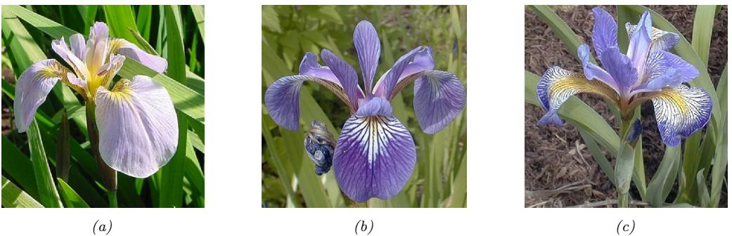
Figure 1.1: Three types of Iris flowers: Setosa, Versicolor and Virginica. Used with kind permission of Dennis Kramb and SIGNA.

index	sl	sw	pl	pw	label
0	5.1	3.5	1.4	0.2	Setosa
1	4.9	3.0	1.4	0.2	Setosa
	···
50	7.0	3.2	4.7	1.4	Versicolor
	···
149	5.9	3.0	5.1	1.8	Virginica

Table 1.1: A subset of the Iris design matrix. The features are: sepal length, sepal width, petal length, petal width. There are 50 examples of each class.

covariates, or predictors; this is often a fixed-dimensional vector of numbers, such as the height and weight of a person, or the pixels in an image. In this case, ^{X = RD}, where ^D is the dimensionality of the vector (i.e., the number of input features). The output y is also known as the label, target, or response. 2 The experience ^E is given in the form of a set of ^N input-output pairs ^{D =} {(xn, ^yn)}^{N n}=1, known as the training set. (N is called the sample size.) The performance measure P depends on the type of output we are predicting, as we discuss below.

1.2.1 Classification

In classification problems, the output space is a set of C unordered and mutually exclusive labels known as classes, Y = {1, 2,…,C}. The problem of predicting the class label given an input is also called pattern recognition. (If there are just two classes, often denoted by y → {0, 1} or y → {↑1, +1}, it is called binary classification.)

1.2.1.1 Example: classifying Iris flowers

As an example, consider the problem of classifying Iris flowers into their 3 subspecies, Setosa, Versicolor and Virginica. Figure 1.1 shows one example of each of these classes.

^2. Sometimes (e.g., in the statsmodels Python package) x are called the exogenous variables and y are called the endogenous variables.

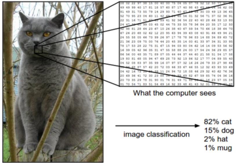
Figure 1.2: Illustration of the image classification problem. From https: // cs231n. github. io/ . Used with kind permission of Andrej Karpathy.

In image classification, the input space X is the set of images, which is a very high-dimensional space: for a color image with ^C = 3 channels (e.g., RGB) and ^{D1 ↓ D2} pixels, we have ^X = ^RD, where D = C ↓ D¹ ↓ D2. (In practice we represent each pixel intensity with an integer, typically from the range {0, 1,…, 255}, but we assume real valued inputs for notational simplicity.) Learning a mapping f : X ↔︎ Y from images to labels is quite challenging, as illustrated in Figure 1.2. However, it can be tackled using certain kinds of functions, such as a convolutional neural network or CNN, which we discuss in Section 14.1.

Fortunately for us, some botanists have already identified 4 simple, but highly informative, numeric features — sepal length, sepal width, petal length, petal width — which can be used to distinguish the three kinds of Iris flowers. In this section, we will use this much lower-dimensional input space, ^{X = R4}, for simplicity. The Iris dataset is a collection of 150 labeled examples of Iris flowers, 50 of each type, described by these 4 features. It is widely used as an example, because it is small and simple to understand. (We will discuss larger and more complex datasets later in the book.)

When we have small datasets of features, it is common to store them in an N ↓ D matrix, in which each row represents an example, and each column represents a feature. This is known as a design matrix; see Table 1.1 for an example.3

The Iris dataset is an example of tabular data. When the inputs are of variable size (e.g., sequences of words, or social networks), rather than fixed-length vectors, the data is usually stored

^3. This particular design matrix has N = 150 rows and D = 4 columns, and hence has a tall and skinny shape, since N → D. By contrast, some datasets (e.g., genomics) have more features than examples, D → N; their design matrices are short and fat. The term “big data” usually means that N is large, whereas the term “wide data” means that D is large (relative to N).

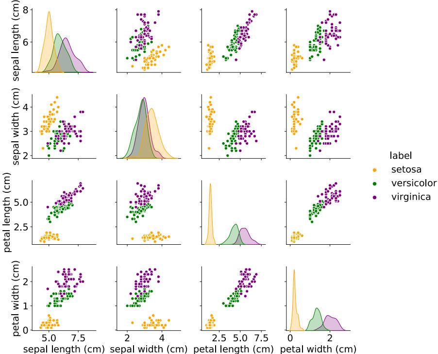
Figure 1.3: Visualization of the Iris data as a pairwise scatter plot. On the diagonal we plot the marginal distribution of each feature for each class. The o!-diagonals contain scatterplots of all possible pairs of features. Generated by iris\_plot.ipynb

in some other format rather than in a design matrix. However, such data is often converted to a fixed-sized feature representation (a process known as featurization), thus implicitly creating a design matrix for further processing. We give an example of this in Section 1.5.4.1, where we discuss the “bag of words” representation for sequence data.

1.2.1.2 Exploratory data analysis

Before tackling a problem with ML, it is usually a good idea to perform exploratory data analysis, to see if there are any obvious patterns (which might give hints on what method to choose), or any obvious problems with the data (e.g., label noise or outliers).

For tabular data with a small number of features, it is common to make a pair plot, in which panel (i, j) shows a scatter plot of variables i and j, and the diagonal entries (i, i) show the marginal density of variable i; all plots are optionally color coded by class label — see Figure 1.3 for an example.

For higher-dimensional data, it is common to first perform dimensionality reduction, and then

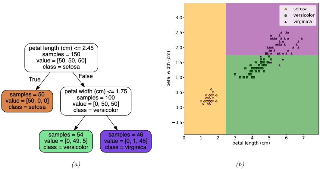
Figure 1.4: Example of a decision tree of depth 2 applied to the Iris data, using just the petal length and petal width features. Leaf nodes are color coded according to the predicted class. The number of training samples that pass from the root to a node is shown inside each box; we show how many values of each class fall into this node. This vector of counts can be normalized to get a distribution over class labels for each node. We can then pick the majority class. Adapted from Figures 6.1 and 6.2 of [Gér19]. Generated by iris\_dtree.ipynb.

to visualize the data in 2d or 3d. We discuss methods for dimensionality reduction in Chapter 20.

1.2.1.3 Learning a classifier

From Figure 1.3, we can see that the Setosa class is easy to distinguish from the other two classes. For example, suppose we create the following decision rule:

\[f(x; \theta) = \begin{cases} \text{Setosa if petal length} < 2.45\\ \text{Versicolor or Viginica otherwise} \end{cases} \tag{1.1}\]

This is a very simple example of a classifier, in which we have partitioned the input space into two regions, defined by the one-dimensional (1d) decision boundary at xpetal length = 2.45. Points lying to the left of this boundary are classified as Setosa; points to the right are either Versicolor or Virginica.

We see that this rule perfectly classifies the Setosa examples, but not the Virginica and Versicolor ones. To improve performance, we can recursively partition the space, by splitting regions in which the classifier makes errors. For example, we can add another decision rule, to be applied to inputs that fail the first test, to check if the petal width is below 1.75cm (in which case we predict Versicolor) or above (in which case we predict Virginica). We can arrange these nested rules into a tree structure,

			Estimate
		Setosa	Versicolor	Virginica
	Setosa	0	1	1
Truth	Versicolor	1	0	1
	Virginica	10	10	0

Table 1.2: Hypothetical asymmetric loss matrix for Iris classification.

called a decision tree, as shown in Figure 1.4a This induces the 2d decision surface shown in Figure 1.4b.

We can represent the tree by storing, for each internal node, the feature index that is used, as well as the corresponding threshold value. We denote all these parameters by ω. We discuss how to learn these parameters in Section 18.1.

1.2.1.4 Empirical risk minimization

The goal of supervised learning is to automatically come up with classification models such as the one shown in Figure 1.4a, so as to reliably predict the labels for any given input. A common way to measure performance on this task is in terms of the misclassification rate on the training set:

\[\mathcal{L}(\boldsymbol{\theta}) \triangleq \frac{1}{N} \sum\_{n=1}^{N} \mathbb{I}\left(y\_n \neq f(\mathbf{z}\_n; \boldsymbol{\theta})\right) \tag{1.2}\]

where I(e) is the binary indicator function, which returns 1 i! (if and only if) the condition e is true, and returns 0 otherwise, i.e.,

\[\mathbb{I}(e) = \begin{cases} 1 & \text{if } e \text{ is true} \\ 0 & \text{if } e \text{ is false} \end{cases} \tag{1.3}\]

This assumes all errors are equal. However it may be the case that some errors are more costly than others. For example, suppose we are foraging in the wilderness and we find some Iris flowers. Furthermore, suppose that Setosa and Versicolor are tasty, but Virginica is poisonous. In this case, we might use the asymmetric loss function ω(y, yˆ) shown in Table 1.2.

We can then define empirical risk to be the average loss of the predictor on the training set:

\[\mathcal{L}(\boldsymbol{\theta}) \triangleq \frac{1}{N} \sum\_{n=1}^{N} \ell(y\_n, f(\boldsymbol{x}\_n; \boldsymbol{\theta})) \tag{1.4}\]

We see that the misclassification rate Equation (1.2) is equal to the empirical risk when we use zero-one loss for comparing the true label with the prediction:

\[\ell\_{01}(y,\hat{y}) = \mathbb{I}\left(y \neq \hat{y}\right) \tag{1.5}\]

See Section 5.1 for more details.

One way to define the problem of model fitting or training is to find a setting of the parameters that minimizes the empirical risk on the training set:

\[\hat{\boldsymbol{\theta}} = \underset{\boldsymbol{\theta}}{\operatorname{argmin}} \mathcal{L}(\boldsymbol{\theta}) = \underset{\boldsymbol{\theta}}{\operatorname{argmin}} \frac{1}{N} \sum\_{n=1}^{N} \ell(y\_n, f(\boldsymbol{x}\_n; \boldsymbol{\theta})) \tag{1.6}\]

This is called empirical risk minimization.

However, our true goal is to minimize the expected loss on future data that we have not yet seen. That is, we want to generalize, rather than just do well on the training set. We discuss this important point in Section 1.2.3.

1.2.1.5 Uncertainty

[We must avoid] false confidence bred from an ignorance of the probabilistic nature of the world, from a desire to see black and white where we should rightly see gray. — Immanuel Kant, as paraphrased by Maria Konnikova [Kon20].

In many cases, we will not be able to perfectly predict the exact output given the input, due to lack of knowledge of the input-output mapping (this is called epistemic uncertainty or model uncertainty), and/or due to intrinsic (irreducible) stochasticity in the mapping (this is called aleatoric uncertainty or data uncertainty).

Representing uncertainty in our prediction can be important for various applications. For example, let us return to our poisonous flower example, whose loss matrix is shown in Table 1.2. If we predict the flower is Virginica with high probability, then we should not eat the flower. Alternatively, we may be able to perform an information gathering action, such as performing a diagnostic test, to reduce our uncertainty. For more information about how to make optimal decisions in the presence of uncertainty, see Section 5.1.

We can capture our uncertainty using the following conditional probability distribution:

\[p(y = c | \mathbf{z}; \boldsymbol{\theta}) = f\_c(\mathbf{z}; \boldsymbol{\theta}) \tag{1.7}\]

where ^f : ^{X ↔︎} [0, 1]^C maps inputs to a probability distribution over the ^C possible output labels. Since ^fc(x; ^ω) returns the probability of class label ^c, we require ⁰ ↘ ^fc ↘ ¹ for each ^c, and $^{C c}=1 f^c = 1. To avoid this restriction, it is common to instead require the model to return unnormalized logprobabilities. We can then convert these to probabilities using the softmax function, which is defined as follows

\[\text{softmax}(\mathbf{a}) \triangleq \left[ \frac{e^{a\_1}}{\sum\_{c'=1}^{C} e^{a\_{c'}}}, \dots, \frac{e^{a\_C}}{\sum\_{c'=1}^{C} e^{a\_{c'}}} \right] \tag{1.8}\]

This maps ^RC to [0, 1]^C , and satisfies the constraints that ⁰ ↘ softmax(a)^c ↘ ¹ and $^{C c}=1 softmax(a)^c = 1. The inputs to the softmax, a = f(x; ω), are called logits. See Section 2.5.2 for details. We thus define the overall model as follows:

\[p(y = c | \mathbf{z}; \boldsymbol{\theta}) = \text{softmax}\_{\mathbf{c}}(f(\mathbf{z}; \boldsymbol{\theta})) \tag{1.9}\]

A common special case of this arises when f is an a!ne function of the form

\[f(\mathbf{z}; \boldsymbol{\theta}) = b + \mathbf{w}^{\mathsf{T}} \mathbf{z} = b + w\_1 x\_1 + w\_2 x\_2 + \dots + w\_D x\_D \tag{1.10}\]

where ω = (b, w) are the parameters of the model. This model is called logistic regression, and will be discussed in more detail in Chapter 10.

In statistics, the w parameters are usually called regression coe!cients (and are typically denoted by ε) and b is called the intercept. In ML, the parameters w are called the weights and b is called the bias. This terminology arises from electrical engineering, where we view the function f as a circuit which takes in x and returns f(x). Each input is fed to the circuit on “wires”, which have weights w. The circuit computes the weighted sum of its inputs, and adds a constant bias or o!set term b. (This use of the term “bias” should not be confused with the statistical concept of bias discussed in Section 4.7.6.1.)

To reduce notational clutter, it is common to absorb the bias term b into the weights w by defining w˜ = [b, w1,…,wD] and defining x˜ = [1, x1,…,xD], so that

\[ \bar{w}^{\mathsf{T}}\bar{x} = b + w^{\mathsf{T}}x\tag{1.11} \]

This converts the a”ne function into a linear function. We will usually assume that this has been done, so we can just write the prediction function as follows:

\[f(x; w) = w^{\top} x\]

1.2.1.6 Maximum likelihood estimation

When fitting probabilistic models, it is common to use the negative log probability as our loss function:

\[\ell(y, f(x; \theta)) = -\log p(y|f(x; \theta)) \tag{1.13}\]

The reasons for this are explained in Section 5.1.6.1, but the intuition is that a good model (with low loss) is one that assigns a high probability to the true output y for each corresponding input x. The average negative log probability of the training set is given by

\[\text{NLL}(\theta) = -\frac{1}{N} \sum\_{n=1}^{N} \log p(y\_n | f(x\_n; \theta)) \tag{1.14}\]

This is called the negative log likelihood. If we minimize this, we can compute the maximum likelihood estimate or MLE:

\[\hat{\theta}\_{\text{mle}} = \underset{\theta}{\text{argmin}} \,\text{NLL}(\theta) \tag{1.15}\]

This is a very common way to fit models to data, as we will see.

1.2.2 Regression

Now suppose that we want to predict a real-valued quantity y → R instead of a class label y → {1,…,C}; this is known as regression. For example, in the case of Iris flowers, y might be the degree of toxicity if the flower is eaten, or the average height of the plant.

Regression is very similar to classification. However, since the output is real-valued, we need to use a di!erent loss function. For regression, the most common choice is to use quadratic loss, or ω² loss:

\[\ell\_2(y, \hat{y}) = (y - \hat{y})^2 \tag{1.16}\]

This penalizes large residuals ^{y ↑ yˆ} more than small ones.4 The empirical risk when using quadratic loss is equal to the mean squared error or MSE:

\[\text{MSE}(\theta) = \frac{1}{N} \sum\_{n=1}^{N} (y\_n - f(x\_n; \theta))^2 \tag{1.17}\]

Based on the discussion in Section 1.2.1.5, we should also model the uncertainty in our prediction. In regression problems, it is common to assume the output distribution is a Gaussian or normal. As we explain in Section 2.6, this distribution is defined by

\[\mathcal{N}(y|\mu,\sigma^2) \stackrel{\Delta}{=} \frac{1}{\sqrt{2\pi\sigma^2}} e^{-\frac{1}{2\sigma^2}(y-\mu)^2} \tag{1.18}\]

where ^µ is the mean, ^ε2 is the variance, and ^≃ 2ϑε² is the normalization constant needed to ensure the density integrates to 1. In the context of regression, we can make the mean depend on the inputs by defining µ = f(xn; ω). We therefore get the following conditional probability distribution:

\[p(y\_n|x\_n; \theta) = \mathcal{N}(y\_n|f(x\_n; \theta), \sigma^2) \tag{1.19}\]

If we assume that the variance ε² is fixed (for simplicity), the corresponding average (per-sample) negative log likelihood becomes

\[\text{NLL}(\boldsymbol{\theta}) = -\frac{1}{N} \sum\_{n=1}^{N} \log \left[ \left( \frac{1}{2\pi\sigma^2} \right)^{\frac{1}{2}} \exp \left( -\frac{1}{2\sigma^2} (y\_n - f(\boldsymbol{x}\_n; \boldsymbol{\theta}))^2 \right) \right] \tag{1.20}\]

\[\hat{\sigma} = \frac{1}{2\sigma^2} \text{MSE}(\hat{\theta}) + \text{const} \tag{1.21}\]

We see that the NLL is proportional to the MSE. Hence computing the maximum likelihood estimate of the parameters will result in minimizing the squared error, which seems like a sensible approach to model fitting.

1.2.2.1 Linear regression

As an example of a regression model, consider the 1d data in Figure 1.5a. We can fit this data using a simple linear regression model of the form

\[f(x; \theta) = b + wx \tag{1.22}\]

^4. If the data has outliers, the quadratic penalty can be too severe. In such cases, it can be better to use ω¹ loss instead, which is more robust. See Section 11.6 for details.

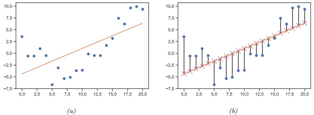
Figure 1.5: (a) Linear regression on some 1d data. (b) The vertical lines denote the residuals between the observed output value for each input (blue circle) and its predicted value (red cross). The goal of least squares regression is to pick a line that minimizes the sum of squared residuals. Generated by linreg\_residuals\_plot.ipynb.

where w is the slope, b is the o”set, and ω = (w, b) are all the parameters of the model. By adjusting ω, we can minimize the sum of squared errors, shown by the vertical lines in Figure 1.5b. until we find the least squares solution

\[\hat{\boldsymbol{\theta}} = \underset{\boldsymbol{\theta}}{\text{argmin}} \,\text{MSE}(\boldsymbol{\theta})\tag{1.23}\]

See Section 11.2.2.1 for details.

If we have multiple input features, we can write

\[f(\mathbf{z}; \boldsymbol{\theta}) = b + w\_1 x\_1 + \dots + w\_D x\_D = b + \mathbf{w}^\mathsf{T} \mathbf{z} \tag{1.24}\]

where ω = (w, b). This is called multiple linear regression.

For example, consider the task of predicting temperature as a function of 2d location in a room. Figure 1.6(a) plots the results of a linear model of the following form:

\[f(x; \theta) = b + w\_1 x\_1 + w\_2 x\_2 \tag{1.25}\]

We can extend this model to use D > 2 input features (such as time of day), but then it becomes harder to visualize.

1.2.2.2 Polynomial regression

The linear model in Figure 1.5a is obviously not a very good fit to the data. We can improve the fit by using a polynomial regression model of degree D. This has the form f(x; w) = w^Tϑ(x), where ϑ(x) is a feature vector derived from the input, which has the following form:

\[\phi(x) = [1, x, x^2, \dots, x^D] \tag{1.26}\]

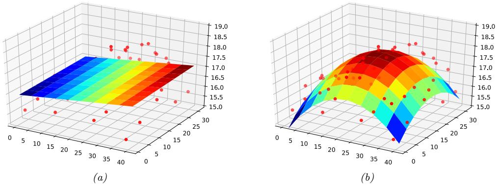
Figure 1.6: Linear and polynomial regression applied to 2d data. Vertical axis is temperature, horizontal axes are location within a room. Data was collected by some remote sensing motes at Intel’s lab in Berkeley, CA (data courtesy of Romain Thibaux). (a) The fitted plane has the form ˆf(x) = w⁰ + w1x¹ + w2x2. (b) Temperature data is fitted with a quadratic of the form ˆf(x) = w⁰ + w1x¹ + w2x² + w3x^{2 1} + w4x^{2 2}. Generated by linreg\_2d\_surface\_demo.ipynb.

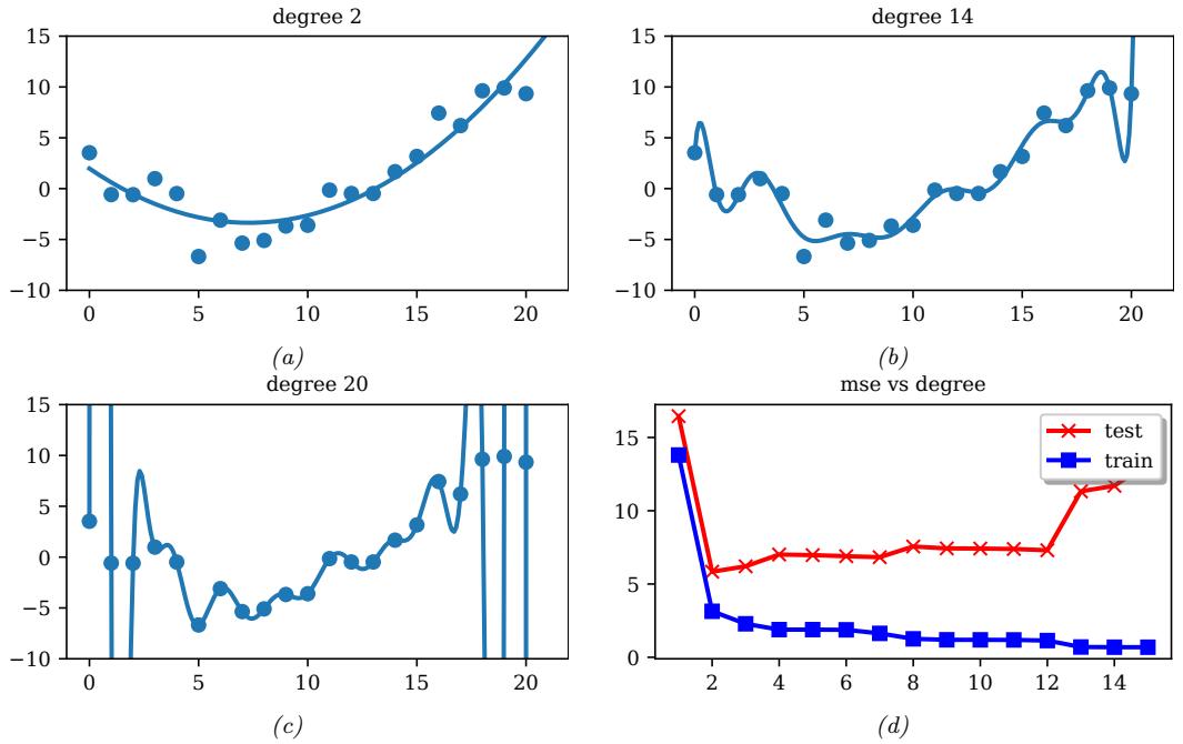
Figure 1.7: (a-c) Polynomials of degrees 2, 14 and 20 fit to 21 datapoints (the same data as in Figure 1.5). (d) MSE vs degree. Generated by linreg\_poly\_vs\_degree.ipynb.

This is a simple example of feature preprocessing, also called feature engineering.

In Figure 1.7a, we see that using D = 2 results in a much better fit. We can keep increasing D, and hence the number of parameters in the model, until D = N ↑ 1; in this case, we have one parameter per data point, so we can perfectly interpolate the data. The resulting model will have 0 MSE, as shown in Figure 1.7c. However, intuitively the resulting function will not be a good predictor for future inputs, since it is too “wiggly”. We discuss this in more detail in Section 1.2.3.

We can also apply polynomial regression to multi-dimensional inputs. For example, Figure 1.6(b) plots the predictions for the temperature model after performing a quadratic expansion of the inputs

\[f(\mathbf{z}; \mathbf{w}) = w\_0 + w\_1 x\_1 + w\_2 x\_2 + w\_3 x\_1^2 + w\_4 x\_2^2 \tag{1.27}\]

The quadratic shape is a better fit to the data than the linear model in Figure 1.6(a), since it captures the fact that the middle of the room is hotter. We can also add cross terms, such as x1x2, to capture interaction e!ects. See Section 1.5.3.2 for details.

Note that the above models still use a prediction function that is a linear function of the parameters w, even though it is a nonlinear function of the original input x. The reason this is important is that a linear model induces an MSE loss function MSE(ω) that has a unique global optimum, as we explain in Section 11.2.2.1.

1.2.2.3 Deep neural networks

In Section 1.2.2.2, we manually specified the transformation of the input features, namely polynomial expansion, ϑ(x) = [1, x1, x2, x² 1, x^{2 2},…]. We can create much more powerful models by learning to do such nonlinear feature extraction automatically. If we let ϑ(x) have its own set of parameters, say V, then the overall model has the form

\[f(x; w, \mathbf{V}) = w^{\top} \phi(x; \mathbf{V}) \tag{1.28}\]

We can recursively decompose the feature extractor ϑ(x; V) into a composition of simpler functions. The resulting model then becomes a stack of L nested functions:

\[f(\mathbf{z}; \boldsymbol{\theta}) = f\_L(f\_{L-1}(\cdots(f\_1(\mathbf{z}))\cdots))\tag{1.29}\]

where fω(x) = f(x; ωω) is the function at layer ω. The final layer is linear and has the form fL(x) = w^{T L}x, so f(x; ω) = w^{T L}f1:L→¹(x), where f1:L→¹(x) = f^L→¹(···(f1(x))···) is the learned feature extractor. This is the key idea behind deep neural networks or DNNs, which includes common variants such as convolutional neural networks (CNNs) for images, and recurrent neural networks (RNNs) for sequences. See Part III for details.

1.2.3 Overfitting and generalization

We can rewrite the empirical risk in Equation (1.4) in the following equivalent way:

\[\mathcal{L}(\boldsymbol{\theta}; \mathcal{D}\_{\text{train}}) = \frac{1}{|\mathcal{D}\_{\text{train}}|} \sum\_{(\mathfrak{x}, \mathfrak{y}) \in \mathcal{D}\_{\text{train}}} \ell(\mathfrak{y}, f(\mathfrak{x}; \boldsymbol{\theta})) \tag{1.30}\]

where |Dtrain| is the size of the training set Dtrain. This formulation is useful because it makes explicit which dataset the loss is being evaluated on.

1.2. Supervised learning 13

With a suitably flexible model, we can drive the training loss to zero (assuming no label noise), by simply memorizing the correct output for each input. For example, Figure 1.7(c) perfectly interpolates the training data (modulo the last point on the right). But what we care about is prediction accuracy on new data, which may not be part of the training set. A model that perfectly fits the training data, but which is too complex, is said to su!er from overfitting.

To detect if a model is overfitting, let us assume (for now) that we have access to the true (but unknown) distribution p↓(x, y) used to generate the training set. Then, instead of computing the empirical risk we compute the theoretical expected loss or population risk

\[\mathcal{L}(\theta; p^\*) \triangleq \mathbb{E}\_{p^\*(x, y)} \left[ \ell(y, f(x; \theta)) \right] \tag{1.31}\]

The di!erence L(ω; p↓) ↑ L(ω; Dtrain) is called the generalization gap. If a model has a large generalization gap (i.e., low empirical risk but high population risk), it is a sign that it is overfitting.

In practice we don’t know p↓. However, we can partition the data we do have into two subsets, known as the training set and the test set. Then we can approximate the population risk using the test risk:

\[\mathcal{L}(\boldsymbol{\theta}; \mathcal{D}\_{\text{test}}) \stackrel{\scriptstyle \Delta}{=} \frac{1}{|\mathcal{D}\_{\text{test}}|} \sum\_{(\mathfrak{x}, \mathfrak{y}) \in \mathcal{D}\_{\text{test}}} \ell(\boldsymbol{y}, f(\boldsymbol{x}; \boldsymbol{\theta})) \tag{1.32}\]

As an example, in Figure 1.7d, we plot the training error and test error for polynomial regression as a function of degree D. We see that the training error goes to 0 as the model becomes more complex. However, the test error has a characteristic U-shaped curve: on the left, where D = 1, the model is underfitting; on the right, where D ⇐ 1, the model is overfitting; and when D = 2, the model complexity is “just right”.

How can we pick a model of the right complexity? If we use the training set to evaluate di!erent models, we will always pick the most complex model, since that will have the most degrees of freedom, and hence will have minimum loss. So instead we should pick the model with minimum test loss.

In practice, we need to partition the data into three sets, namely the training set, the test set and a validation set; the latter is used for model selection, and we just use the test set to estimate future performance (the population risk), i.e., the test set is not used for model fitting or model selection. See Section 4.5.4 for further details.

1.2.4 No free lunch theorem

All models are wrong, but some models are useful. — George Box [BD87, p424].5

Given the large variety of models in the literature, it is natural to wonder which one is best. Unfortunately, there is no single best model that works optimally for all kinds of problems — this is sometimes called the no free lunch theorem [Wol96]. The reason is that a set of assumptions (also called inductive bias) that works well in one domain may work poorly in another. The best way to pick a suitable model is based on domain knowledge, and/or trial and error (i.e., using model selection techniques such as cross validation (Section 4.5.4) or Bayesian methods (Section 5.2.2 and Section 5.2.6). For this reason, it is important to have many models and algorithmic techniques in one’s toolbox to choose from.

^5. George Box is a retired statistics professor at the University of Wisconsin.

1.3 Unsupervised learning

In supervised learning, we assume that each input example x in the training set has an associated set of output targets y, and our goal is to learn the input-output mapping. Although this is useful, and can be di”cult, supervised learning is essentially just “glorified curve fitting” [Pea18].

An arguably much more interesting task is to try to “make sense of” data, as opposed to just learning a mapping. That is, we just get observed “inputs” D = {xⁿ : n =1: N} without any corresponding “outputs” yn. This is called unsupervised learning.

From a probabilistic perspective, we can view the task of unsupervised learning as fitting an unconditional model of the form p(x), which can generate new data x, whereas supervised learning involves fitting a conditional model, p(y|x), which specifies (a distribution over) outputs given inputs.6

Unsupervised learning avoids the need to collect large labeled datasets for training, which can often be time consuming and expensive (think of asking doctors to label medical images).

Unsupervised learning also avoids the need to learn how to partition the world into often arbitrary categories. For example, consider the task of labeling when an action, such as “drinking” or “sipping”, occurs in a video. Is it when the person picks up the glass, or when the glass first touches the mouth, or when the liquid pours out? What if they pour out some liquid, then pause, then pour again — is that two actions or one? Humans will often disagree on such issues [Idr+17], which means the task is not well defined. It is therefore not reasonable to expect machines to learn such mappings.7

Finally, unsupervised learning forces the model to “explain” the high-dimensional inputs, rather than just the low-dimensional outputs. This allows us to learn richer models of “how the world works”. As Geo! Hinton, who is a famous professor of ML at the University of Toronto, has said:

When we’re learning to see, nobody’s telling us what the right answers are — we just look. Every so often, your mother says “that’s a dog”, but that’s very little information. You’d be lucky if you got a few bits of information — even one bit per second — that way. The brain’s visual system has O(1014) neural connections. And you only live for O(109) seconds. So it’s no use learning one bit per second. You need more like O(105) bits per second. And there’s only one place you can get that much information: from the input itself. — Geo!rey Hinton, 1996 (quoted in [Gor06]).

1.3.1 Clustering

A simple example of unsupervised learning is the problem of finding clusters in data. The goal is to partition the input into regions that contain “similar” points. As an example, consider a 2d version of the Iris dataset. In Figure 1.8a, we show the points without any class labels. Intuitively there are at least two clusters in the data, one in the bottom left and one in the top right. Furthermore, if we assume that a “good” set of clusters should be fairly compact, then we might want to split the top right into (at least) two subclusters. The resulting partition into three clusters is shown in Figure 1.8b. (Note that there is no correct number of clusters; instead, we need to consider the

^6. In the statistics community, it is common to use x to denote exogenous variables that are not modeled, but are simply given as inputs. Therefore an unconditional model would be denoted p(y) rather than p(x).

^7. A more reasonable approach is to try to capture the probability distribution over labels produced by a “crowd” of annotators (see e.g., [Dum+18; Aro+19]). This embraces the fact that there can be multiple “correct” labels for a given input due to the ambiguity of the task itself.

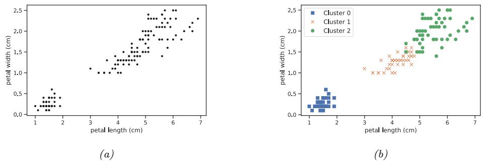
Figure 1.8: (a) A scatterplot of the petal features from the iris dataset. (b) The result of unsupervised clustering using K = 3. Generated by iris\_kmeans.ipynb.

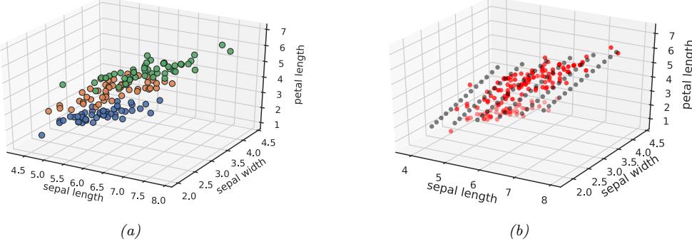
Figure 1.9: (a) Scatterplot of iris data (first 3 features). Points are color coded by class. (b) We fit a 2d linear subspace to the 3d data using PCA. The class labels are ignored. Red dots are the original data, black dots are points generated from the model using xˆ = Wz + µ, where z are latent points on the underlying inferred 2d linear manifold. Generated by iris\_pca.ipynb.

tradeo! between model complexity and fit to the data. We discuss ways to make this tradeo! in Section 21.3.7.)

1.3.2 Discovering latent “factors of variation”

When dealing with high-dimensional data, it is often useful to reduce the dimensionality by projecting it to a lower dimensional subspace which captures the “essence” of the data. One approach to this problem is to assume that each observed high-dimensional output ^{xn → RD} was generated by a set of hidden or unobserved low-dimensional latent factors ^{zn → RK}. We can represent the model diagrammatically as follows: zⁿ ↔︎ xn, where the arrow represents causation. Since we don’t know the latent factors zn, we often assume a simple prior probability model for p(zn) such as a Gaussian, which says that each factor is a random K-dimensional vector. If the data is real-valued, we can use a Gaussian likelihood as well.

The simplest example is when we use a linear model, p(xn|zn; ω) = N (xn|Wzⁿ + µ, !). The resulting model is called factor analysis (FA). It is similar to linear regression, except we only observe the outputs xn, and not the inputs zn. In the special case that ! = ε²I, this reduces to a model called probabilistic principal components analysis (PCA), which we will explain in Section 20.1. In Figure 1.9, we give an illustration of how this method can find a 2d linear subspace when applied to some simple 3d data.

Of course, assuming a linear mapping from zⁿ to xⁿ is very restrictive. However, we can create nonlinear extensions by defining ^p(xn|zn; ^ω) = ^N (xn|f(zn; ^ω), ^ε2I), where ^f(z; ^ω) is a nonlinear model, such as a deep neural network. It becomes much harder to fit such a model (i.e., to estimate the parameters ω), because the inputs to the neural net have to be inferred, as well as the parameters of the model. However, there are various approximate methods, such as the variational autoencoder which can be applied (see Section 20.3.5).

1.3.3 Self-supervised learning

A recently popular approach to unsupervised learning is known as self-supervised learning. In this approach, we create proxy supervised tasks from unlabeled data. For example, we might try to learn to predict a color image from a grayscale image, or to mask out words in a sentence and then try to predict them given the surrounding context. The hope is that the resulting predictor xˆ¹ = f(x2; ω), where x² is the observed input and xˆ¹ is the predicted output, will learn useful features from the data, that can then be used in standard, downstream supervised tasks. This avoids the hard problem of trying to infer the “true latent factors” z behind the observed data, and instead relies on standard supervised learning methods. We discuss this approach in more detail in Section 19.2.

1.3.4 Evaluating unsupervised learning

Although unsupervised learning is appealing, it is very hard to evaluate the quality of the output of an unsupervised learning method, because there is no ground truth to compare to [TOB16].

A common method for evaluating unsupervised models is to measure the probability assigned by the model to unseen test examples. We can do this by computing the (unconditional) negative log likelihood of the data:

\[\mathcal{L}(\boldsymbol{\theta}; \mathcal{D}) = -\frac{1}{|\mathcal{D}|} \sum\_{\boldsymbol{x} \in \mathcal{D}} \log p(\boldsymbol{x}|\boldsymbol{\theta}) \tag{1.33}\]

This treats the problem of unsupervised learning as one of density estimation. The idea is that a good model will not be “surprised” by actual data samples (i.e., will assign them high probability). Furthermore, since probabilities must sum to 1.0, if the model assigns high probability to regions of data space where the data samples come from, it implicitly assigns low probability to the regions where the data does not come from. Thus the model has learned to capture the typical patterns in the data. This can be used inside of a data compression algorithm.

Unfortunately, density estimation is di”cult, especially in high dimensions. Furthermore, a model that assigns high probability to the data may not have learned useful high-level patterns (after all, the model could just memorize all the training examples).

An alternative evaluation metric is to use the learned unsupervised representation as features or input to a downstream supervised learning method. If the unsupervised method has discovered useful

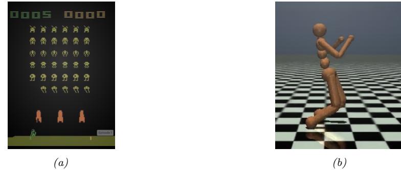
Figure 1.10: Examples of some control problems. (a) Space Invaders Atari game. From https: // gymnasium. farama. org/ environments/ atari/ space\_ invaders/ . (b) Controlling a humanoid robot in the MuJuCo simulator so it walks as fast as possible without falling over. From https: // gymnasium. farama. org/ environments/ mujoco/ humanoid/ .

patterns, then it should be possible to use these patterns to perform supervised learning using much less labeled data than when working with the original features. For example, in Section 1.2.1.1, we saw how the 4 manually defined features of iris flowers contained most of the information needed to perform classification. We were thus able to train a classifier with nearly perfect performance using just 150 examples. If the input was raw pixels, we would need many more examples to achieve comparable performance (see Section 14.1). That is, we can increase the sample e!ciency of learning (i.e., reduce the number of labeled examples needed to get good performance) by first learning a good representation.

Increased sample e”ciency is a useful evaluation metric, but in many applications, especially in science, the goal of unsupervised learning is to gain understanding, not to improve performance on some prediction task. This requires the use of models that are interpretable, but which can also generate or “explain” most of the observed patterns in the data. To paraphrase Plato, the goal is to discover how to “carve nature at its joints”. Of course, evaluating whether we have successfully discovered the true underlying structure behind some dataset often requires performing experiments and thus interacting with the world. We discuss this topic further in Section 1.4.

1.4 Reinforcement learning

In addition to supervised and unsupervised learning, there is a third kind of ML known as reinforcement learning (RL). In this class of problems, the system or agent has to learn how to interact with its environment. This can be encoded by means of a policy a = ϑ(x), which specifies which action to take in response to each possible input x (derived from the environment state).

For example, consider an agent that learns to play a video game, such as Atari Space Invaders (see Figure 1.10a). In this case, the input x is the image (or sequence of past images), and the output a is the direction to move in (left or right) and whether to fire a missile or not. As a more complex example, consider the problem of a robot learning to walk (see Figure 1.10b). In this case, the input x is the set of joint positions and angles for all the limbs, and the output a is a set of actuation or motor control signals.

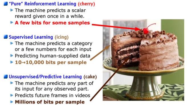
Figure 1.11: The three types of machine learning visualized as layers of a chocolate cake. This figure (originally from https: // bit. ly/ 2m65Vs1 ) was used in a talk by Yann LeCun at NIPS’16, and is used with his kind permission.

The di!erence from supervised learning (SL) is that the system is not told which action is the best one to take (i.e., which output to produce for a given input). Instead, the system just receives an occasional reward (or punishment) signal in response to the actions that it takes. This is like learning with a critic, who gives an occasional thumbs up or thumbs down, as opposed to learning with a teacher, who tells you what to do at each step.

RL has grown in popularity recently, due to its broad applicability (since the reward signal that the agent is trying to optimize can be any metric of interest). However, it can be harder to make RL work than it is for supervised or unsupervised learning, for a variety of reasons. A key di”culty is that the reward signal may only be given occasionally (e.g., if the agent eventually reaches a desired state), and even then it may be unclear to the agent which of its many actions were responsible for getting the reward. (Think of playing a game like chess, where there is a single win or lose signal at the end of the game.)

To compensate for the minimal amount of information coming from the reward signal, it is common to use other information sources, such as expert demonstrations, which can be used in a supervised way, or unlabeled data, which can be used by an unsupervised learning system to discover the underlying structure of the environment. This can make it feasible to learn from a limited number of trials (interactions with the environment). As Yann LeCun put it, in an invited talk at the NIPS8 conference in 2016: “If intelligence was a cake, unsupervised learning would be the chocolate sponge, supervised learning would be the icing, and reinforcement learning would be the cherry.” This is illustrated in Figure 1.11.

More information on RL can be found in the sequel to this book, [Mur23].

^8. NIPS stands for “Neural Information Processing Systems”. It is one of the premier ML conferences. It has recently been renamed to NeurIPS.

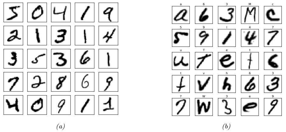
Figure 1.12: (a) Visualization of the MNIST dataset. Each image is 28 → 28. There are 60k training examples and 10k test examples. We show the first 25 images from the training set. Generated by mnist\_viz\_tf.ipynb. (b) Visualization of the EMNIST dataset. There are 697,932 training examples, and 116,323 test examples, each of size 28 → 28. There are 62 classes (a-z, A-Z, 0-9). We show the first 25 images from the training set. Generated by emnist\_viz\_jax.ipynb.

1.5 Data

Machine learning is concerned with fitting models to data using various algorithms. Although we focus on the modeling and algorithm aspects, it is important to mention that the nature and quality of the training data also plays a vital role in the success of any learned model.

In this section, we briefly describe some common image and text datasets that we will use in this book. We also briefly discuss the topic of data preprocessing.

1.5.1 Some common image datasets

In this section, we briefly discuss some image datasets that we will use in this book.

1.5.1.1 Small image datasets

One of the simplest and most widely used is known as MNIST [LeC+98; YB19].9 This is a dataset of 60k training images and 10k test images, each of size 28 ↓ 28 (grayscale), illustrating handwritten digits from 10 categories. Each pixel is an integer in the range {0, 1,…, 255}; these are usually rescaled to [0, 1], to represent pixel intensity. We can optionally convert this to a binary image by thresholding. See Figure 1.12a for an illustration.

MNIST is so widely used in the ML community that Geo! Hinton, a famous ML researcher, has called it the “drosophila of machine learning”, since if we cannot make a method work well on MNIST, it will likely not work well on harder datasets. However, nowadays MNIST classification is considered

^9. The term “MNIST” stands for “Modified National Institute of Standards”; The term “modified” is used because the images have been preprocessed to ensure the digits are mostly in the center of the image.

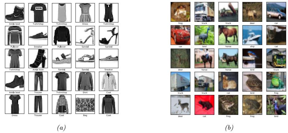
Figure 1.13: (a) Visualization of the Fashion-MNIST dataset [XRV17]. The dataset has the same size as MNIST, but is harder to classify. There are 10 classes: T-shirt/top, Trouser, Pullover, Dress, Coat, Sandal, Shirt, Sneaker, Bag, Ankle-boot. We show the first 25 images from the training set. Generated by fashion\_viz\_tf.ipynb. (b) Some images from the CIFAR-10 dataset [KH09]. Each image is 32 → 32 → 3, where the final dimension of size 3 refers to RGB. There are 50k training examples and 10k test examples. There are 10 classes: plane, car, bird, cat, deer, dog, frog, horse, ship, and truck. We show the first 25 images from the training set. Generated by cifar\_viz\_tf.ipynb.

“too easy”, since it is possible to distinguish most pairs of digits by looking at just a single pixel. Various extensions have been proposed.

In [Coh+17], they proposed EMNIST (extended MNIST), that also includes lower and upper case letters. See Figure 1.12b for a visualization. This dataset is much harder than MNIST, since there are 62 classes, several of which are quite ambiguous (e.g., the digit 1 vs the lower case letter l).

In [XRV17], they proposed Fashion-MNIST, which has exactly the same size and shape as MNIST, but where each image is the picture of a piece of clothing instead of a handwritten digit. See Figure 1.13a for a visualization.

For small color images, the most common dataset is CIFAR [KH09].10 This is a dataset of 60k images, each of size 32↓32↓3, representing everyday objects from 10 or 100 classes; see Figure 1.13b for an illustration.11

1.5.1.2 ImageNet

Small datasets are useful for prototyping ideas, but it is also important to test methods on larger datasets, both in terms of image size and number of labeled examples. The most widely used dataset

^10. CIFAR stands for “Canadian Institute For Advanced Research”. This is the agency that funded labeling of the dataset, which was derived from the TinyImages dataset at http://groups.csail.mit.edu/vision/TinyImages/ created by Antonio Torralba. See [KH09] for details.

^11. Despite its popularity, the CIFAR dataset has some issues. For example, the base error on CIFAR-100 is 5.85% due to mislabeling [NAM21]. This makes any results with accuracy above 94.15% acc suspicious. Also, 10% of CIFAR-100 training set images are duplicated in the test set [BD20].

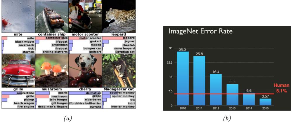
Figure 1.14: (a) Sample images from the ImageNet dataset [Rus+15]. This subset consists of 1.3M color training images, each of which is 256 → 256 pixels in size. There are 1000 possible labels, one per image, and the task is to minimize the top-5 error rate, i.e., to ensure the correct label is within the 5 most probable predictions. Below each image we show the true label, and a distribution over the top 5 predicted labels. If the true label is in the top 5, its probability bar is colored red. Predictions are generated by a convolutional neural network (CNN) called “AlexNet” (Section 14.3.2). From Figure 4 of [KSH12]. Used with kind permission of Alex Krizhevsky. (b) Misclassification rate (top 5) on the ImageNet competition over time. Used with kind permission of Andrej Karpathy.

of this type is called ImageNet [Rus+15]. This is a dataset of ⇒ 14M images of size 256 ↓ 256 ↓ 3 illustrating various objects from 20,000 classes; see Figure 1.14a for some examples.

The ImageNet dataset was used as the basis of the ImageNet Large Scale Visual Recognition Challenge (ILSVRC), which ran from 2010 to 2018. This used a subset of 1.3M images from 1000 classes. During the course of the competition, significant progress was made by the community, as shown in Figure 1.14b. In particular, 2015 marked the first year in which CNNs could outperform humans (or at least one human, namely Andrej Karpathy) at the task of classifying images from ImageNet. Note that this does not mean that CNNs are better at vision than humans (see e.g., [YL21] for some common failure modes). Instead, it mostly likely reflects the fact that the dataset makes many fine-grained classification distinctions — such as between a “tiger” and a “tiger cat” — that humans find di”cult to understand; by contrast, su”ciently flexible CNNs can learn arbitrary patterns, including random labels [Zha+17a].

Although ImageNet is much harder than MNIST and CIFAR as a classification benchmark, it too is almost “saturated” [Bey+20]. Nevertheless, relative performance of methods on ImageNet is often a surprisingly good predictor of performance on other, unrelated image classification tasks (see e.g., [Rec+19]), so it remains very widely used.

1.5.2 Some common text datasets

Machine learning is often applied to text to solve a variety of tasks. This is known as natural language processing or NLP (see e.g., [JM20] for details). Below we briefly mention a few text

Table 1.3: We show snippets of the first two sentences from the IMDB movie review dataset. The first example is labeled positive and the second negative. ( refers to an unknown token.)

datasets that we will use in this book.

1.5.2.1 Text classification

A simple NLP task is text classification, which can be used for email spam classification, sentiment analysis (e.g., is a movie or product review positive or negative), etc. A common dataset for evaluating such methods is the IMDB movie review dataset from [Maa+11]. (IMDB stands for “Internet Movie Database”.) This contains 25k labeled examples for training, and 25k for testing. Each example has a binary label, representing a positive or negative rating. See Table 1.3 for some example sentences.

1.5.2.2 Machine translation

A more di”cult NLP task is to learn to map a sentence x in one language to a “semantically equivalent” sentence y in another language; this is called machine translation. Training such models requires aligned (x, y) pairs. Fortunately, several such datasets exist, e.g., from the Canadian parliament (English-French pairs), and the European Union (Europarl). A subset of the latter, known as the WMT dataset (Workshop on Machine Translation), consists of English-German pairs, and is widely used as a benchmark dataset.

1.5.2.3 Other seq2seq tasks

A generalization of machine translation is to learn a mapping from one sequence x to any other sequence y. This is called a seq2seq model, and can be viewed as a form of high-dimensional classification (see Section 15.2.3 for details). This framing of the problem is very general, and includes many tasks, such as document summarization, question answering, etc. For example, Table 1.4 shows how to formulate question answering as a seq2seq problem: the input is the text T and question Q, and the output is the answer A, which is a set of words, possibly extracted from the input.

1.5.2.4 Language modeling

The rather grandiose term “language modeling” refers to the task of creating unconditional generative models of text sequences, p(x1,…,x^T ). This only requires input sentences x, without any corresponding “labels” y. We can therefore think of this as a form of unsupervised learning, which we discuss in Section 1.3. If the language model generates output in response to an input, as in seq2seq, we can regard it as a conditional generative model.

^1. this film was just brilliant casting location scenery story direction everyone’s really suited the part they played robert is an amazing actor …

^2. big hair big boobs bad music and a giant safety pin these are the words to best describe this terrible movie i love cheesy horror movies and i’ve seen hundreds…

T: In meteorology, precipitation is any product of the condensation of atmospheric water vapor that falls under gravity. The main forms of precipitation include drizzle, rain, sleet, snow, graupel and hail… Precipitation forms as smaller droplets coalesce via collision with other rain drops or ice crystals within a cloud. Short, intense periods of rain in scattered locations are called “showers”.

• Q1: What causes precipitation to fall? A1: gravity
• Q2: What is another main form of precipitation besides drizzle, rain, snow, sleet and hail? A2: graupel
• Q3: Where do water droplets collide with ice crystals to form precipitation? A3: within a cloud

Table 1.4: Question-answer pairs for a sample passage in the SQuAD dataset. Each of the answers is a segment of text from the passage. This can be solved using sentence pair tagging. The input is the paragraph text T and the question Q. The output is a tagging of the relevant words in T that answer the question in Q. From Figure 1 of [Raj+16]. Used with kind permission of Percy Liang.

1.5.3 Preprocessing discrete input data

Many ML models assume that the data consists of real-valued feature vectors, ^{x → RD}. However, sometimes the input may have discrete input features, such as categorical variables like race and gender, or words from some vocabulary. In the sections below, we discuss some ways to preprocess such data to convert it to vector form. This is a common operation that is used for many di!erent kinds of models.

1.5.3.1 One-hot encoding

When we have categorical features, we need to convert them to a numerical scale, so that computing weighted combinations of the inputs makes sense. The standard way to preprocess such categorical variables is to use a one-hot encoding, also called a dummy encoding. If a variable x has K values, we will denote its dummy encoding as follows: one-hot(x)=[I(x = 1),…,I(x = K)]. For example, if there are 3 colors (say red, green and blue), the corresponding one-hot vectors will be one-hot(red) = [1, 0, 0], one-hot(green) = [0, 1, 0], and one-hot(blue) = [0, 0, 1].

1.5.3.2 Feature crosses

A linear model using a dummy encoding for each categorical variable can capture the main e”ects of each variable, but cannot capture interaction e”ects between them. For example, suppose we want to predict the fuel e”ciency of a vehicle given two categorical input variables: the type (say SUV, Truck, or Family car), and the country of origin (say USA or Japan). If we concatenate the one-hot encodings for the ternary and binary features, we get the following input encoding:

\[\phi(x) = \left[ 1, \mathbb{I}\left(x\_1 = S\right), \mathbb{I}\left(x\_1 = T\right), \mathbb{I}\left(x\_1 = F\right), \mathbb{I}\left(x\_2 = U\right), \mathbb{I}\left(x\_2 = J\right) \right] \tag{1.34}\]

where x¹ is the type and x² is the country of origin.

This model cannot capture dependencies between the features. For example, we expect trucks to be less fuel e”cient, but perhaps trucks from the USA are even less e”cient than trucks from Japan. This cannot be captured using the linear model in Equation (1.34) since the contribution from the country of origin is independent of the car type.

We can fix this by computing explicit feature crosses. For example, we can define a new composite feature with 3 ↓ 2 possible values, to capture the interaction of type and country of origin. The new model becomes

\[\begin{aligned} f(x; w) &= w^\top \phi(x) \\ &= w\_0 + w\_1 \mathbb{I}\left(x\_1 = S\right) + w\_2 \mathbb{I}\left(x\_1 = T\right) + w\_3 \mathbb{I}\left(x\_1 = F\right) \\ &+ w\_4 \mathbb{I}\left(x\_2 = U\right) + w\_5 \mathbb{I}\left(x\_2 = J\right) \\ &+ w\_6 \mathbb{I}\left(x\_1 = S, x\_2 = U\right) + w\_7 \mathbb{I}\left(x\_1 = T, x\_2 = U\right) + w\_8 \mathbb{I}\left(x\_1 = F, x\_2 = U\right) \\ &+ w\_9 \mathbb{I}\left(x\_1 = S, x\_2 = J\right) + w\_{10} \mathbb{I}\left(x\_1 = T, x\_2 = J\right) + w\_{11} \mathbb{I}\left(x\_1 = F, x\_2 = J\right) \end{aligned} \tag{1.36}\]

We can see that the use of feature crosses converts the original dataset into a wide format, with many more columns.

1.5.4 Preprocessing text data

In Section 1.5.2, we briefly discussed text classification and other NLP tasks. To feed text data into a classifier, we need to tackle various issues. First, documents have a variable length, and are thus not fixed-length feature vectors, as assumed by many kinds of models. Second, words are categorical variables with many possible values (equal to the size of the vocabulary), so the corresponding one-hot encodings will be very high-dimensional, with no natural notion of similarity. Third, we may encounter words at test time that have not been seen during training (so-called out-of-vocabulary or OOV words). We discuss some solutions to these problems below. More details can be found in e.g., [BKL10; MRS08; JM20].

1.5.4.1 Bag of words model

A simple approach to dealing with variable-length text documents is to interpret them as a bag of words, in which we ignore word order. To convert this to a vector from a fixed input space, we first map each word to a token from some vocabulary.

To reduce the number of tokens, we often use various pre-processing techniques such as the following: dropping punctuation, converting all words to lower case; dropping common but uninformative words, such as “and” and “the” (this is called stop word removal); replacing words with their base form, such as replacing “running” and “runs” with “run” (this is called word stemming); etc. For details, see e.g., [BL12], and for some sample code, see text\_preproc\_jax.ipynb.

Let xnt be the token at location t in the n’th document. If there are D unique tokens in the vocabulary, then we can represent the n’th document as a D-dimensional vector x˜n, where x˜nv is the number of times that word v occurs in document n:

\[\bar{x}\_{nv} = \sum\_{t=1}^{T} \mathbb{I}\left(x\_{nt} = v\right) \tag{1.37}\]

where T is the length of document n. We can now interpret documents as vectors in R^D. This is called the vector space model of text [SWY75; TP10].

We traditionally store input data in an N ↓ D design matrix denoted by X, where D is the number of features. In the context of vector space models, it is more common to represent the input data

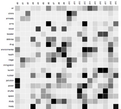
Figure 1.15: Example of a term-document matrix, where raw counts have been replaced by their TF-IDF values (see Section 1.5.4.2). Darker cells are larger values. Used with kind permission of Christoph Carl Kling.

as a D ↓ N term frequency matrix, where TFij is the frequency of term i in document j. See Figure 1.15 for an illustration.

1.5.4.2 TF-IDF

One problem with representing documents as word count vectors is that frequent words may have undue influence, just because the magnitude of their word count is higher, even if they do not carry much semantic content. A common solution to this is to transform the counts by taking logs, which reduces the impact of words that occur many times within a single document.

To reduce the impact of words that occur many times in general (across all documents), we compute a quantity called the inverse document frequency, defined as follows: IDFⁱ ↭ log ^N 1+DFⁱ , where DFⁱ is the number of documents with term i. We can combine these transformations to compute the TF-IDF matrix as follows:

\[\text{TFIDF}\_{ij} = \log(\text{TF}\_{ij} + 1) \times \text{IDF}\_i \tag{1.38}\]

(We often normalize each row as well.) This provides a more meaningful representation of documents, and can be used as input to many ML algorithms. See tfidf\_demo.ipynb for an example.

1.5.4.3 Word embeddings

Although the TF-IDF transformation improves on raw count vectors by placing more weight on “informative” words and less on “uninformative” words, it does not solve the fundamental problem with the one-hot encoding (from which count vectors are derived), which is that that semantically similar words, such as “man” and “woman”, may be not be any closer (in vector space) than semantically dissimilar words, such as “man” and “banana”. Thus the assumption that points that are close in input space should have similar outputs, which is implicitly made by most prediction models, is invalid.

The standard way to solve this problem is to use word embeddings, in which we map each sparse one-hot vector, ^xnt ^→ {0, 1}^V , to a lower-dimensional dense vector, ^ent ^{→ RK} using ^ent = Exnt, where ^{E → R}K↔︎^V is learned such that semantically similar words are placed close by. There are many ways to learn such embeddings, as we discuss in Section 20.5.

Once we have an embedding matrix, we can represent a variable-length text document as a bag of word embeddings. We can then convert this to a fixed length vector by summing (or averaging) the embeddings:

\[\overline{\mathbf{e}}\_{n} = \sum\_{t=1}^{T} \mathbf{e}\_{nt} = \mathbf{E} \widetilde{\mathbf{x}}\_{n} \tag{1.39}\]

where x˜ⁿ is the bag of words representation from Equation (1.37). We can then use this inside of a logistic regression classifier, which we briefly introduced in Section 1.2.1.5. The overall model has the form

\[p(y = c | \mathbf{x}\_n, \boldsymbol{\theta}) = \text{softmax}\_c(\mathbf{W} \mathbf{E} \bar{x}\_n) \tag{1.40}\]

We often use a pre-trained word embedding matrix E, in which case the model is linear in W, which simplifies parameter estimation (see Chapter 10). See also Section 15.7 for a discussion of contextual word embeddings.

1.5.4.4 Dealing with novel words

At test time, the model may encounter a completely novel word that it has not seen before. This is known as the out of vocabulary or OOV problem. Such novel words are bound to occur, because the set of words is an open class. For example, the set of proper nouns (names of people and places) is unbounded.

A standard heuristic to solve this problem is to replace all novel words with the special symbol UNK, which stands for “unknown”. However, this loses information. For example, if we encounter the word “athazagoraphobia”, we may guess it means “fear of something”, since phobia is a common su”x in English (derived from Greek) to mean “fear of”. (It turns out that athazagoraphobia means “fear of being forgotten about or ignored”.)

We could work at the character level, but this would require the model to learn how to group common letter combinations together into words. It is better to leverage the fact that words have substructure, and then to take as input subword units or wordpieces [SHB16; Wu+16]; these are often created using a method called byte-pair encoding [Gag94], which is a form of data compression that creates new symbols to represent common substrings.

1.5.5 Handling missing data

Sometimes we may have missing data, in which parts of the input x or output y may be unknown. If the output is unknown during training, the example is unlabeled; we consider such semi-supervised learning scenarios in Section 19.3. We therefore focus on the case where some of the input features may be missing, either at training or testing time, or both.

To model this, let M be an N ↓ D matrix of binary variables, where Mnd = 1 if feature d in example n is missing, and Mnd = 0 otherwise. Let X^v be the visible parts of the input feature matrix,

corresponding to Mnd = 0, and X^h be the missing parts, corresponding to Mnd = 1. Let Y be the output label matrix, which we assume is fully observed. If we assume p(M|Xv, Xh, Y) = p(M), we say the data is missing completely at random or MCAR, since the missingness does not depend on the hidden or observed features. If we assume p(M|Xv, Xh, Y) = p(M|Xv, Y), we say the data is missing at random or MAR, since the missingness does not depend on the hidden features, but may depend on the visible features. If neither of these assumptions hold, we say the data is not missing at random or NMAR.

In the MCAR and MAR cases, we can ignore the missingness mechanism, since it tells us nothing about the hidden features. However, in the NMAR case, we need to model the missing data mechanism, since the lack of information may be informative. For example, the fact that someone did not fill out an answer to a sensitive question on a survey (e.g., “Do you have COVID?”) could be informative about the underlying value. See e.g., [LR87; Mar08] for more information on missing data models.

In this book, we will always make the MAR assumption. However, even with this assumption, we cannot directly use a discriminative model, such as a DNN, when we have missing input features, since the input x will have some unknown values.

A common heuristic is called mean value imputation, in which missing values are replaced by their empirical mean. More generally, we can fit a generative model to the input, and use that to fill in the missing values. We briefly discuss some suitable generative models for this task in Chapter 20, and in more detail in the sequel to this book, [Mur23].

1.6 Discussion

In this section, we situate ML and this book into a larger context.

1.6.1 The relationship between ML and other fields

There are several subcommunities that work on ML-related topics, each of which have di!erent names. The field of predictive analytics is similar to supervised learning (in particular, classification and regression), but focuses more on business applications. Data mining covers both supervised and unsupervised machine learning, but focuses more on structured data, usually stored in large commercial databases. Data science uses techniques from machine learning and statistics, but also emphasizes other topics, such as data integration, data visualization, and working with domain experts, often in an iterative feedback loop (see e.g., [BS17]). The di!erence between these areas is often just one of terminology.12

ML is also very closely related to the field of statistics. Indeed, Jerry Friedman, a famous statistics professor at Stanford, said13

[If the statistics field had] incorporated computing methodology from its inception as a fundamental tool, as opposed to simply a convenient way to apply our existing tools, many of the other data related fields [such as ML] would not have needed to exist — they would have been part of statistics. — Jerry Friedman [Fri97b]

^12. See https://developers.google.com/machine-learning/glossary/ for a useful “ML glossary”.

^13. Quoted in https://brenocon.com/blog/2008/12/statistics-vs-machine-learning-fight/

Machine learning is also related to artificial intelligence (AI). Historically, the field of AI assumed that we could program “intelligence” by hand (see e.g., [RN10; PM17]), but this approach has largely failed to live up to expectations, mostly because it proved to be too hard to explicitly encode all the knowledge such systems need. Consequently, there is renewed interest in using ML to help an AI system acquire its own knowledge. (Indeed the connections are so close that sometimes the terms “ML” and “AI” are used interchangeably, although this is arguably misleading [Pre21].)

1.6.2 Structure of the book

We have seen that ML is closely related to many other subjects in mathematics, statistics, computer science, etc. It can be hard to know where to start.

In this book, we take one particular path through this interconnected landscape, using probability theory as our unifying lens. We cover statistical foundations in Part I, supervised learning in Part II–Part IV, and unsupervised learning in Part V. For more information on these (and other) topics, please see the sequel to this book, [Mur23],

In addition to the book, you may find the online Python notebooks that accompany this book helpful. See <probml.github.io/book1> for details.

1.6.3 Caveats

In this book, we will see how machine learning can be used to create systems that can (attempt to) predict outputs given inputs. These predictions can then be used to choose actions so as to minimize expected loss. When designing such systems, it can be hard to design a loss function that correctly specifies all of our preferences; this can result in “reward hacking” in which the machine optimizes the reward function we give it, but then we realize that the function did not capture various constraints or preferences that we forgot to specify [Wei76; Amo+16; D’A+20]. (This is particularly important when tradeo!s need to be made between multiple objectives.)

Reward hacking is an example of a larger problem known as the “alignment problem” [Chr20], which refers to the potential discrepancy between what we ask our algorithms to optimize and what we actually want them to do for us; this has raised various concerns in the context of AI ethics and AI safety (see e.g., [KR19; Lia20; Spe+22]). Russell [Rus19] proposes to solve this problem by not explicitly specifying a reward function, but instead forcing the machine to infer the reward by observing human behavior, an approach known as inverse reinforcement learning (IRL). Of course, emulating current or past human behavior too closely may be undesirable, and can be biased by the data that is available for training (see e.g., [Pau+20]).

The above view of AI, in which an “intelligent” system makes decisions on its own, without a human in the loop, is believed by many to be the path towards “artificial general intelligence” or AGI. An alternative approach is to view AI as “augmented intelligence” (sometimes called intelligence augmentation or IA). In this paradigm, AI is a process for creating “smart tools”, like adaptive cruise control or auto-complete in search engines; such tools maintain a human in the decision-making loop. In this framing, systems which have AI/ML components in them are not that di!erent from other complex, semi-autonomous human artefacts, such as aeroplanes with autopilot, online trading platforms or medical diagnostic systems (c.f. [Jor19; Ace]). Of course, as the AI tools become more powerful, they can end up doing more and more on their own, making this approach similar to AGI. However, in augmented intelligence, the goal is not to emulate or exceed human

behavior at certain tasks, but instead to help humans get stu! done more easily; this is how we treat most other technologies [Kap16].

The IRL approach of [Rus19] is one way to formalize this. Specifically, the human and machine are both treated as agents in a two-player cooperative game, called an “assistance game”, where the machine’s goal is to maximize the user’s utility (reward) function, which is inferred based on the human’s behavior. This way, if the machine is uncertain about whether something is a good idea or not, it will proceed cautiously (e.g., by asking the user for their preference), rather than blindly solving the wrong problem. (See [Mur23] for more details on reinforcement learning and related topics.)

Part I

Foundations

2 Probability: Univariate Models

2.1 Introduction

In this chapter, we give a brief introduction to the basics of probability theory. There are many good books that go into more detail, e.g., [GS97; BT08; Cha21].

2.1.1 What is probability?

Probability theory is nothing but common sense reduced to calculation. — Pierre Laplace, 1812

We are all comfortable saying that the probability that a (fair) coin will land heads is 50%. But what does this mean? There are actually two di!erent interpretations of probability. One is called the frequentist interpretation. In this view, probabilities represent long run frequencies of events that can happen multiple times. For example, the above statement means that, if we flip the coin many times, we expect it to land heads about half the time.1

The other interpretation is called the Bayesian interpretation of probability. In this view, probability is used to quantify our uncertainty or ignorance about something; hence it is fundamentally related to information rather than repeated trials [Jay03; Lin06]. In the Bayesian view, the above statement means we believe the coin is equally likely to land heads or tails on the next toss.

One big advantage of the Bayesian interpretation is that it can be used to model our uncertainty about one-o! events that do not have long term frequencies. For example, we might want to compute the probability that the polar ice cap will melt by 2030 CE. This event will happen zero or one times, but cannot happen repeatedly. Nevertheless, we ought to be able to quantify our uncertainty about this event; based on how probable we think this event is, we can decide how to take the optimal action, as discussed in Chapter 5. We shall therefore adopt the Bayesian interpretation in this book. Fortunately, the basic rules of probability theory are the same, no matter which interpretation is adopted.

2.1.2 Types of uncertainty

The uncertainty in our predictions can arise for two fundamentally di!erent reasons. The first is due to our ignorance of the underlying hidden causes or mechanism generating our data. This is

^1. Actually, the Stanford statistician (and former professional magician) Persi Diaconis has shown that a coin is about 51% likely to land facing the same way up as it started, due to the physics of the problem [DHM07].

called epistemic uncertainty, since epistemology is the philosophical term used to describe the study of knowledge. However, a simpler term for this is model uncertainty. The second kind of uncertainty arises from intrinsic variability, which cannot be reduced even if we collect more data. This is sometimes called aleatoric uncertainty [Hac75; KD09], derived from the Latin word for “dice”, although a simpler term would be data uncertainty. As a concrete example, consider tossing a fair coin. We might know for sure that the probability of heads is p = 0.5, so there is no epistemic uncertainty, but we still cannot perfectly predict the outcome.

This distinction can be important for applications such as active learning. A typical strategy is to query examples for which H(p(y|x, D)) is large (where H(p) is the entropy, discussed in Section 6.1). However, this could be due to uncertainty about the parameters, i.e., large H(p(ω|D)), or just due to inherent variability of the outcome, corresponding to large entropy of p(y|x, ω). In the latter case, there would not be much use collecting more samples, since our uncertainty would not be reduced. See [Osb16] for further discussion of this point.

2.1.3 Probability as an extension of logic

In this section, we review the basic rules of probability, following the presentation of [Jay03], in which we view probability as an extension of Boolean logic.

2.1.3.1 Probability of an event

We define an event, denoted by the binary variable A, as some state of the world that either holds or does not hold. For example, A might be event “it will rain tomorrow”, or “it rained yesterday”, or “the label is y = 1”, or “the parameter ϖ is between 1.5 and 2.0”, etc. The expression Pr(A) denotes the probability with which you believe event A is true (or the long run fraction of times that A will occur). We require that 0 ↘ Pr(A) ↘ 1, where Pr(A)=0 means the event definitely will not happen, and Pr(A)=1 means the event definitely will happen. We write Pr(A) to denote the probability of event A not happening; this is defined to be Pr(A)=1 ↑ Pr(A).

2.1.3.2 Probability of a conjunction of two events

We denote the joint probability of events A and B both happening as follows:

\[\Pr(A \land B) = \Pr(A, B) \tag{2.1}\]

If A and B are independent events, we have

\[\Pr(A,B) = \Pr(A)\Pr(B) \tag{2.2}\]

For example, suppose X and Y are chosen uniformly at random from the set X = {1, 2, 3, 4}. Let A be the event that X → {1, 2}, and B be the event that Y → {3}. Then we have Pr(A, B) = Pr(A) Pr(B) = ^{1 2} · ¹ 4 .

2.1.3.3 Probability of a union of two events

The probability of event A or B happening is given by

\[\Pr(A \lor B) = \Pr(A) + \Pr(B) - \Pr(A \land B) \tag{2.3}\]

If the events are mutually exclusive (so they cannot happen at the same time), we get

\[\Pr(A \lor B) = \Pr(A) + \Pr(B) \tag{2.4}\]

For example, suppose X is chosen uniformly at random from the set X = {1, 2, 3, 4}. Let A be the event that ^{X →} {1, ²} and ^B be the event that ^{X →} {3}. Then we have Pr(^A ⇓ ^B) = ^{2 4 + 1} 4 .

2.1.3.4 Conditional probability of one event given another

We define the conditional probability of event B happening given that A has occurred as follows:

\[\Pr(B|A) \stackrel{\Delta}{=} \frac{\Pr(A,B)}{\Pr(A)}\tag{2.5}\]

This is not defined if Pr(A)=0, since we cannot condition on an impossible event.

2.1.3.5 Independence of events

We say that event A is independent of event B if

\[\Pr(A,B) = \Pr(A)\Pr(B) \tag{2.6}\]

2.1.3.6 Conditional independence of events

We say that events A and B are conditionally independent given event C if

\[\Pr(A, B|C) = \Pr(A|C)\Pr(B|C) \tag{2.7}\]

This is written as A ⇔ B|C. Events are often dependent on each other, but may be rendered independent if we condition on the relevant intermediate variables, as we discuss in more detail later in this chapter.

2.2 Random variables

Suppose X represents some unknown quantity of interest, such as which way a dice will land when we roll it, or the temperature outside your house at the current time. If the value of X is unknown and/or could change, we call it a random variable or rv. The set of possible values, denoted X , is known as the sample space or state space. An event is a set of outcomes from a given sample space. For example, if X represents the face of a dice that is rolled, so X = {1, 2,…, 6}, the event of “seeing a 1” is denoted X = 1, the event of “seeing an odd number” is denoted X → {1, 3, 5}, the event of “seeing a number between 1 and 3” is denoted 1 ↘ X ↘ 3, etc.

2.2.1 Discrete random variables

If the sample space X is finite or countably infinite, then X is called a discrete random variable. In this case, we denote the probability of the event that X has value x by Pr(X = x). We define the

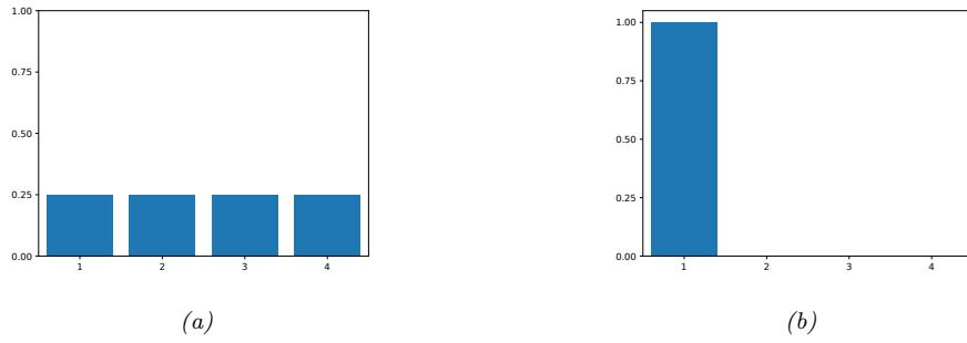
Figure 2.1: Some discrete distributions on the state space X = {1, 2, 3, 4}. (a) A uniform distribution with p(x = k)=1/4. (b) A degenerate distribution (delta function) that puts all its mass on x = 1. Generated by discrete\_prob\_dist\_plot.ipynb.

probability mass function or pmf as a function which computes the probability of events which correspond to setting the rv to each possible value:

\[p(x) \triangleq \Pr(X = x) \tag{2.8}\]

The pmf satisfies the properties ⁰ ↘ ^p(x) ↘ ¹ and $ ^x↑^{X p}(x)=1.

If X has a finite number of values, say K, the pmf can be represented as a list of K numbers, which we can plot as a histogram. For example, Figure 2.1 shows two pmf’s defined on X = {1, 2, 3, 4}. On the left we have a uniform distribution, p(x)=1/4, and on the right, we have a degenerate distribution, p(x) = I(x = 1), where I() is the binary indicator function. Thus the distribution in Figure 2.1(b) represents the fact that X is always equal to the value 1. (Thus we see that random variables can also be constant.)

2.2.2 Continuous random variables

If X → R is a real-valued quantity, it is called a continuous random variable. In this case, we can no longer create a finite (or countable) set of distinct possible values it can take on. However, there are a countable number of intervals which we can partition the real line into. If we associate events with X being in each one of these intervals, we can use the methods discussed above for discrete random variables. Informally speaking, we can represent the probability of X taking on a specific real value by allowing the size of the intervals to shrink to zero, as we show below.

2.2.2.1 Cumulative distribution function (cdf)

Define the events A = (X ↘ a), B = (X ↘ b) and C = (a<X ↘ b), where a<b. We have that B = A ⇓ C, and since A and C are mutually exclusive, the sum rules gives

\[\Pr(B) = \Pr(A) + \Pr(C) \tag{2.9}\]

and hence the probability of being in interval C is given by

\[\Pr(C) = \Pr(B) - \Pr(A) \tag{2.10}\]

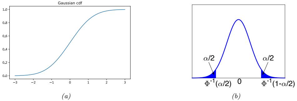
Figure 2.2: (a) Plot of the cdf for the standard normal, N (0, 1). Generated by gauss\_plot.ipynb. (b) Corresponding pdf. The shaded regions each contain ω/2 of the probability mass. Therefore the nonshaded region contains ^{1 ↑ ω} of the probability mass. The leftmost cuto! point is !→¹(ω/2), where ! is the cdf of the Gaussian. By symmetry, the rightmost cuto! point is !→¹(1 ^{↑ ω}/2) = ^↑!→¹(ω/2). Generated by quantile\_plot.ipynb.

In general, we define the cumulative distribution function or cdf of the rv X as follows:

\[P(x) \triangleq \Pr(X \le x) \tag{2.11}\]

(Note that we use a capital P to represent the cdf.) Using this, we can compute the probability of being in any interval as follows:

\[\Pr(a < X \le b) = P(b) - P(a) \tag{2.12}\]

Cdf’s are monotonically non-decreasing functions. See Figure 2.2a for an example, where we illustrate the cdf of a standard normal distribution, N (x|0, 1); see Section 2.6 for details.

2.2.2.2 Probability density function (pdf)

We define the probability density function or pdf as the derivative of the cdf:

\[p(x) \triangleq \frac{d}{dx}P(x) \tag{2.13}\]

(Note that this derivative does not always exist, in which case the pdf is not defined.) See Figure 2.2b for an example, where we illustrate the pdf of a univariate Gaussian (see Section 2.6 for details).

Given a pdf, we can compute the probability of a continuous variable being in a finite interval as follows:

\[\Pr(a < X \le b) = \int\_{a}^{b} p(x) dx = P(b) - P(a) \tag{2.14}\]

As the size of the interval gets smaller, we can write

\[\Pr(x < X \le x + dx) \approx p(x)dx\tag{2.15}\]

Intuitively, this says the probability of X being in a small interval around x is the density at x times the width of the interval.

2.2.2.3 Quantiles

If the cdf P is strictly monotonically increasing, it has an inverse, called the inverse cdf, or percent point function (ppf), or quantile function.

If ^P is the cdf of ^X, then ^{P →}1(q) is the value ^xq such that Pr(^X ↘ ^xq) = ^q; this is called the ^q’th quantile of P. The value P ^→1(0.5) is the median of the distribution, with half of the probability mass on the left, and half on the right. The values P ^→1(0.25) and P ^→1(0.75) are the lower and upper quartiles.

For example, let ! be the cdf of the Gaussian distribution ^N (0, 1), and !→¹ be the inverse cdf. Then points to the left of !→1(ϱ/2) contain ϱ/2 of the probability mass, as illustrated in Figure 2.2b. By symmetry, points to the right of !→¹(1 ^{↑ ϱ}/2) also contain ^ϱ/² of the mass. Hence the central interval (!→¹(ϱ/2), !→¹(1 ^{↑ ϱ}/2)) contains 1 ^{↑ ϱ} of the mass. If we set ^ϱ = 0.05, the central 95% interval is covered by the range

\[(\Phi^{-1}(0.025), \Phi^{-1}(0.975)) = (-1.96, 1.96) \tag{2.16}\]

If the distribution is ^N (µ, ^ε2), then the 95% interval becomes (^{µ ↑ 1}.96ε, µ + 1.96ε). This is often approximated by writing µ ± 2ε.

2.2.3 Sets of related random variables

In this section, we discuss distributions over sets of related random variables.

Suppose, to start, that we have two random variables, X and Y . We can define the joint distribution of two random variables using p(x, y) = p(X = x, Y = y) for all possible values of X and Y . If both variables have finite cardinality, we can represent the joint distribution as a 2d table, all of whose entries sum to one. For example, consider the following example with two binary variables:

\[\begin{array}{c|cc} p(X,Y) & Y=0 & Y=1\\ \hline X=0 & 0.2 & 0.3\\ X=1 & 0.3 & 0.2 \\ \end{array}\]

If two variables are independent, we can represent the joint as the product of the two marginals. If both variables have finite cardinality, we can factorize the 2d joint table into a product of two 1d vectors, as shown in Figure 2.3.

Given a joint distribution, we define the marginal distribution of an rv as follows:

\[p(X=x) = \sum\_{y} p(X=x, Y=y) \tag{2.17}\]

where we are summing over all possible states of Y . This is sometimes called the sum rule or the rule of total probability. We define p(Y = y) similarly. For example, from the above 2d table, we see p(X = 0) = 0.2+0.3=0.5 and p(Y = 0) = 0.2+0.3=0.5. (The term “marginal” comes from the accounting practice of writing the sums of rows and columns on the side, or margin, of a table.)

We define the conditional distribution of an rv using

\[p(Y=y|X=x) = \frac{p(X=x, Y=y)}{p(X=x)}\tag{2.18}\]

We can rearrange this equation to get

\[p(x,y) = p(x)p(y|x) \tag{2.19}\]

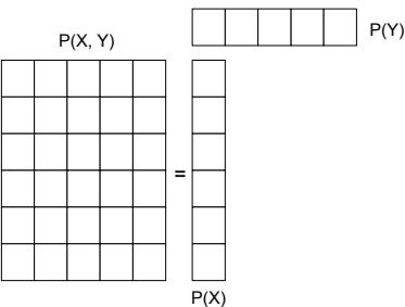
Figure 2.3: Computing p(x, y) = p(x)p(y), where X ↓ Y . Here X and Y are discrete random variables; X has 6 possible states (values) and Y has 5 possible states. A general joint distribution on two such variables would require (6 → 5) ↑ 1 = 29 parameters to define it (we subtract 1 because of the sum-to-one constraint). By assuming (unconditional) independence, we only need (6 ↑ 1) + (5 ↑ 1) = 9 parameters to define p(x, y).

This is called the product rule.

By extending the product rule to D variables, we get the chain rule of probability:

\[p(\mathbf{z}\_{1:D}) = p(x\_1)p(x\_2|x\_1)p(x\_3|x\_1,x\_2)p(x\_4|x\_1,x\_2,x\_3)\dots p(x\_D|\mathbf{z}\_{1:D-1})\tag{2.20}\]

This provides a way to create a high dimensional joint distribution from a set of conditional distributions. We discuss this in more detail in Section 3.6.

2.2.4 Independence and conditional independence

We say X and Y are unconditionally independent or marginally independent, denoted X ⇔ Y , if we can represent the joint as the product of the two marginals (see Figure 2.3), i.e.,

\[X \perp Y \iff p(X, Y) = p(X)p(Y) \tag{2.21}\]

In general, we say a set of variables X1,…,Xⁿ is (mutually) independent if the joint can be written as a product of marginals for all subsets {X1,…,Xm} ′ {X1,…,Xn}: i.e.,

\[p(X\_1, \ldots, X\_m) = \prod\_{i=1}^m p(X\_i) \tag{2.22}\]

For example, we say X1, X2, X³ are mutually independent if the following conditions hold: p(X1, X2, X3) = p(X1)p(X2)p(X3), p(X1, X2) = p(X1)p(X2), p(X2, X3) = p(X2)p(X3), and p(X1, X3) = p(X1)p(X3). 2

Unfortunately, unconditional independence is rare, because most variables can influence most other variables. However, usually this influence is mediated via other variables rather than being direct. We therefore say X and Y are conditionally independent (CI) given Z i! the conditional joint can be written as a product of conditional marginals:

\[X \perp Y \mid Z \iff p(X, Y | Z) = p(X | Z)p(Y | Z) \tag{2.23}\]

^2. For further discussion, see https://github.com/probml/pml-book/issues/353#issuecomment-1120327442.

We can write this assumption as a graph X ↑ Z ↑ Y , which captures the intuition that all the dependencies between X and Y are mediated via Z. By using larger graphs, we can define complex joint distributions; these are known as graphical models, and are discussed in Section 3.6.

2.2.5 Moments of a distribution

In this section, we describe various summary statistics that can be derived from a probability distribution (either a pdf or pmf).

2.2.5.1 Mean of a distribution

The most familiar property of a distribution is its mean, or expected value, often denoted by µ. For continuous rv’s, the mean is defined as follows:

\[\mathbb{E}\left[X\right] \stackrel{\Delta}{=} \int\_{\mathcal{X}} x \, p(x) dx \tag{2.24}\]

If the integral is not finite, the mean is not defined; we will see some examples of this later.

For discrete rv’s, the mean is defined as follows:

\[\mathbb{E}\left[X\right] \stackrel{\Delta}{=} \sum\_{x \in X} x \, p(x) \tag{2.25}\]

However, this is only meaningful if the values of x are ordered in some way (e.g., if they represent integer counts).

Since the mean is a linear operator, we have

\[\mathbb{E}\left[aX + b\right] = a\mathbb{E}\left[X\right] + b\]

This is called the linearity of expectation.

For a set of n random variables, one can show that the expectation of their sum is as follows:

\[\mathbb{E}\left[\sum\_{i=1}^{n} X\_i\right] = \sum\_{i=1}^{n} \mathbb{E}\left[X\_i\right] \tag{2.27}\]

If they are independent, the expectation of their product is given by

\[\mathbb{E}\left[\prod\_{i=1}^{n}X\_{i}\right] = \prod\_{i=1}^{n}\mathbb{E}\left[X\_{i}\right] \tag{2.28}\]

2.2.5.2 Variance of a distribution

The variance is a measure of the “spread” of a distribution, often denoted by ε². This is defined as follows:

\[\mathbb{V}\left[X\right] \stackrel{\Delta}{=} \mathbb{E}\left[(X-\mu)^2\right] = \int (x-\mu)^2 p(x)dx\tag{2.29}\]

\[=\int x^2 p(x)dx + \mu^2 \int p(x)dx - 2\mu \int x p(x)dx = \mathbb{E}\left[X^2\right] - \mu^2\tag{2.30}\]

from which we derive the useful result

\[\mathbb{E}\left[X^2\right] = \sigma^2 + \mu^2\tag{2.31}\]

The standard deviation is defined as

\[\text{std}\left[X\right] \triangleq \sqrt{\mathbb{V}\left[X\right]} = \sigma \tag{2.32}\]

This is useful since it has the same units as X itself.

The variance of a shifted and scaled version of a random variable is given by

\[\mathbb{V}\left[aX + b\right] = a^2 \mathbb{V}\left[X\right] \tag{2.33}\]

If we have a set of n independent random variables, the variance of their sum is given by the sum of their variances:

\[\mathbb{V}\left[\sum\_{i=1}^{n} X\_i\right] = \sum\_{i=1}^{n} \mathbb{V}\left[X\_i\right] \tag{2.34}\]

The variance of their product can also be derived, as follows:

\[\mathbb{E}\left[\prod\_{i=1}^{n}X\_{i}\right] = \mathbb{E}\left[(\prod\_{i}X\_{i})^{2}\right] - (\mathbb{E}\left[\prod\_{i}X\_{i}\right])^{2} \tag{2.35}\]

\[=\mathbb{E}\left[\prod\_{i}X\_{i}^{2}\right]-(\prod\_{i}\mathbb{E}\left[X\_{i}\right])^{2}\tag{2.36}\]

\[\hat{\lambda} = \prod\_{i} \mathbb{E}\left[X\_i^2\right] - \prod\_{i} (\mathbb{E}\left[X\_i\right])^2 \tag{2.37}\]

\[\hat{\lambda} = \prod\_{i} (\mathbb{V}\left[X\_{i}\right] + (\mathbb{E}\left[X\_{i}\right])^{2}) - \prod\_{i} (\mathbb{E}\left[X\_{i}\right])^{2} \tag{2.38}\]

\[=\prod\_{i} (\sigma\_i^2 + \mu\_i^2) - \prod\_{i} \mu\_i^2 \tag{2.39}\]

2.2.5.3 Mode of a distribution

The mode of a distribution is the value with the highest probability mass or probability density:

\[\mathbf{x}^\* = \operatorname\*{argmax}\_{\mathbf{z}} p(\mathbf{z}) \tag{2.40}\]

If the distribution is multimodal, this may not be unique, as illustrated in Figure 2.4. Furthermore, even if there is a unique mode, this point may not be a good summary of the distribution.

2.2.5.4 Conditional moments

When we have two or more dependent random variables, we can compute the moments of one given knowledge of the other. For example, the law of iterated expectations, also called the law of total expectation, tells us that

\[\mathbb{E}\left[X\right] = \mathbb{E}\_Y\left[\mathbb{E}\left[X|Y\right]\right] \tag{2.41}\]

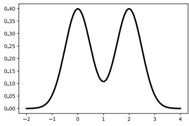
Figure 2.4: Illustration of a mixture of two 1d Gaussians, p(x)=0.5N (x|0, 0.5) + 0.5N (x|2, 0.5). Generated by bimodal\_dist\_plot.ipynb.

To prove this, let us suppose, for simplicity, that X and Y are both discrete rv’s. Then we have

\[\mathbb{E}\_Y\left[\mathbb{E}\left[X|Y\right]\right] = \mathbb{E}\_Y\left[\sum\_x x \, p(X = x|Y)\right] \tag{2.42}\]

\[I = \sum\_{y} \left[ \sum\_{x} x \, p(X = x | Y = y) \right] p(Y = y) = \sum\_{x, y} x p(X = x, Y = y) = \mathbb{E} \left[ X \right] \tag{2.43}\]

To give a more intuitive explanation, consider the following simple example.3 Let X be the lifetime duration of a lightbulb, and let Y be the factory the lightbulb was produced in. Suppose E [X|Y = 1] = 5000 and E [X|Y = 2] = 4000, indicating that factory 1 produces longer lasting bulbs. Suppose factory 1 supplies 60% of the lightbulbs, so p(Y = 1) = 0.6 and p(Y = 2) = 0.4. Then the expected duration of a random lightbulb is given by

\[\mathbb{E}\left[X\right] = \mathbb{E}\left[X|Y=1\right]p(Y=1) + \mathbb{E}\left[X|Y=2\right]p(Y=2) = 5000 \times 0.6 + 4000 \times 0.4 = 4600 \quad \text{(2.44)}\]

There is a similar formula for the variance. In particular, the law of total variance, also called the conditional variance formula, tells us that

\[\mathbb{V}\left[X\right] = \mathbb{E}\_Y\left[\mathbb{V}\left[X|Y\right]\right] + \mathbb{V}\_Y\left[\mathbb{E}\left[X|Y\right]\right] \tag{2.45}\]

To see this, let us define the conditional moments, ^µX|^{Y = E} [X|^Y ], ^sX|^{Y = E + X2}|^Y , , and ε2 ^X|^{Y = V} [X|^Y ] ^{= sX}|^{Y ↑ µ2 X}|^Y , which are functions of ^Y (and therefore are random quantities). Then we have

\[\mathbb{V}\left[X\right] = \mathbb{E}\left[X^2\right] - \left(\mathbb{E}\left[X\right]\right)^2 = \mathbb{E}\_Y\left[s\_{X\midY}\right] - \left(\mathbb{E}\_Y\left[\mu\_{X\midY}\right]\right)^2\tag{2.46}\]

\[=\mathbb{E}\_Y\left[\sigma\_{X\mid Y}^2\right] + \mathbb{E}\_Y\left[\mu\_{X\mid Y}^2\right] - \left(\mathbb{E}\_Y\left[\mu\_{X\mid Y}\right]\right)^2\tag{2.47}\]

\[\mathbb{E} = \mathbb{E}\_Y\left[\mathbb{V}\left[X|Y\right]\right] + \mathbb{V}\_Y\left[\mu\_{X|Y}\right] \tag{2.48}\]

To get some intuition for these formulas, consider a mixture of K univariate Gaussians. Let Y be the hidden indicator variable that specifies which mixture component we are using, and let

^3. This example is from https://en.wikipedia.org/wiki/Law\_of\_total\_expectation, but with modified notation.

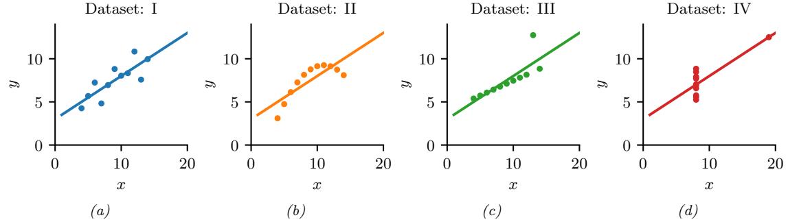
Figure 2.5: Illustration of Anscombe’s quartet. All of these datasets have the same low order summary statistics. Generated by anscombes\_quartet.ipynb.

X = $^{K y}=1 ϑyN (X|µy, εy). In Figure 2.4, we have ϑ¹ = ϑ² = 0.5, µ¹ = 0, µ² = 2, ε¹ = ε² = 0.5. Thus

\[\mathbb{E}\left[\mathbb{V}\left[X|Y\right]\right] = \pi\_1 \sigma\_1^2 + \pi\_2 \sigma\_2^2 = 0.25\tag{2.49}\]

\[\mathbb{V}\left[\mathbb{E}\left[X|Y\right]\right] = \pi\_1(\mu\_1 - \overline{\mu})^2 + \pi\_2(\mu\_2 - \overline{\mu})^2 = 0.5(0 - 1)^2 + 0.5(2 - 1)^2 = 0.5 + 0.5 = 1\tag{2.50}\]

So we get the intuitive result that the variance of X is dominated by which centroid it is drawn from (i.e., di!erence in the means), rather than the local variance around each centroid.

2.2.6 Limitations of summary statistics *

Although it is common to summarize a probability distribution (or points sampled from a distribution) using simple statistics such as the mean and variance, this can lose a lot of information. A striking example of this is known as Anscombe’s quartet [Ans73], which is illustrated in Figure 2.5. This shows 4 di!erent datasets of (x, y) pairs, all of which have identical mean, variance and correlation coe”cient ς (defined in Section 3.1.2): E [x] = 9, V [x] = 11, E [y] = 7.50, V [y] = 4.12, and ς = 0.816. 4 However, the joint distributions p(x, y) from which these points were sampled are clearly very di!erent. Anscombe invented these datasets, each consisting of 10 data points, to counter the impression among statisticians that numerical summaries are superior to data visualization [Ans73].

An even more striking example of this phenomenon is shown in Figure 2.6. This consists of a dataset that looks like a dinosaur5, plus 11 other datasets, all of which have identical low order statistics. This collection of datasets is called the Datasaurus Dozen [MF17]. The exact values of the (x, y) points are available online.6 They were computed using simulated annealing, a derivative free optimization method which we discuss in the sequel to this book, [Mur23]. (The objective

^4. The maximum likelihood estimate for the variance in Equation (4.36) di!ers from the unbiased estimate in Equation (4.38). For the former, we have V [x] = 10.00, V [y] = 3.75, for the latter, we have V [x] = 11.00, V [y] = 4.12. 5. This dataset was created by Alberto Cairo, and is available at http://www.thefunctionalart.com/2016/08/ download-datasaurus-never-trust-summary.html

^6. https://www.autodesk.com/research/publications/same-stats-different-graphs. There are actually 13 datasets in total, including the dinosaur. We omitted the “away” dataset for visual clarity.

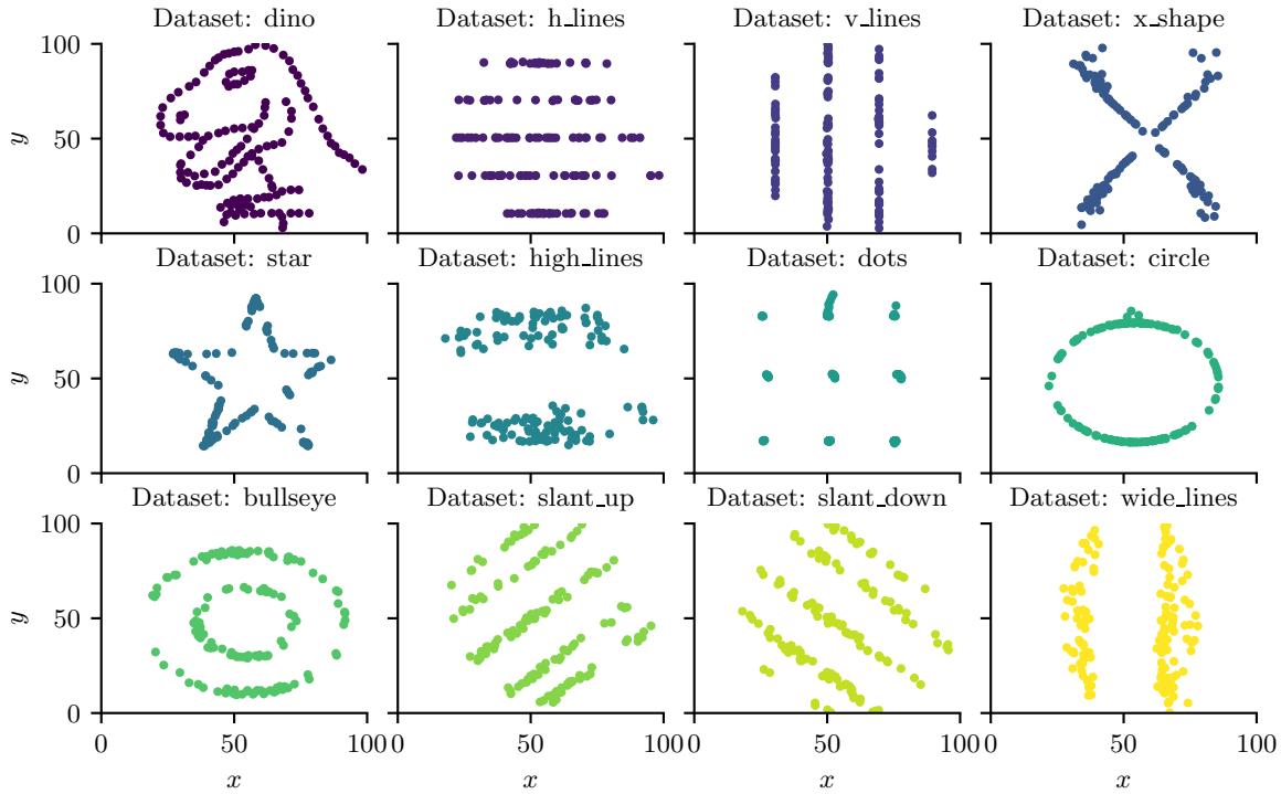
Figure 2.6: Illustration of the Datasaurus Dozen. All of these datasets have the same low order summary statistics. Adapted from Figure 1 of [MF17]. Generated by datasaurus\_dozen.ipynb.

function being optimized measures deviation from the target summary statistics of the original dinosaur, plus distance from a particular target shape.)

The same simulated annealing approach can be applied to 1d datasets, as shown in Figure 2.7. We see that all the datasets are quite di!erent, but they all have the same median and inter-quartile range as shown by the central shaded part of the box plots in the middle. A better visualization is known as a violin plot, shown on the right. This shows (two copies of) the 1d kernel density estimate (Section 16.3) of the distribution on the vertical axis, in addition to the median and IQR markers. This visualization is better able to distinguish di!erences in the distributions. However, the technique is limited to 1d data.

2.3 Bayes’ rule

Bayes’s theorem is to the theory of probability what Pythagoras’s theorem is to geometry. — Sir Harold Je!reys, 1973 [Jef73].

In this section, we discuss the basics of Bayesian inference. According to the Merriam-Webster dictionary, the term “inference” means “the act of passing from sample data to generalizations, usually with calculated degrees of certainty”. The term “Bayesian” is used to refer to inference methods that

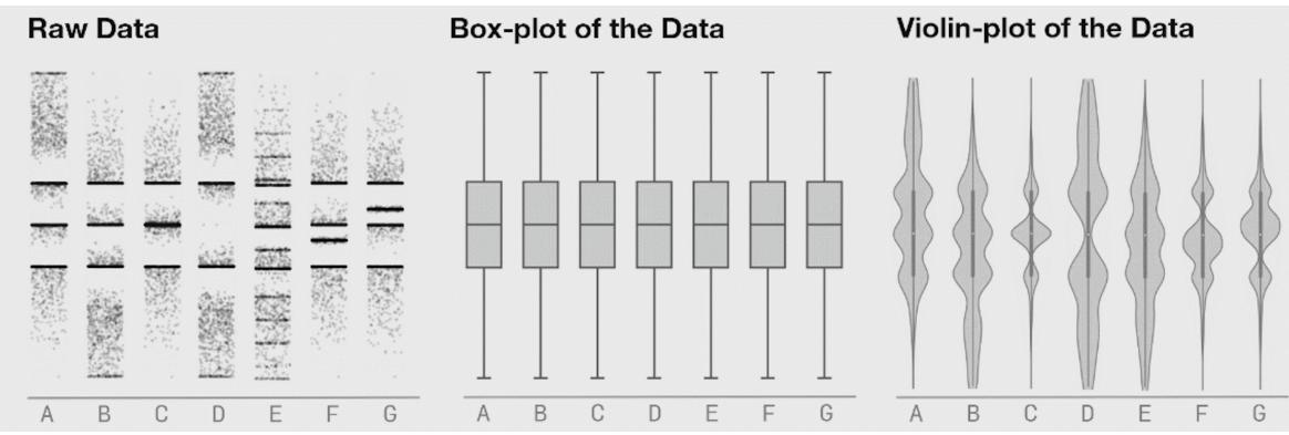
Figure 2.7: Illustration of 7 di!erent datasets (left), the corresponding box plots (middle) and violin box plots (right). From Figure 8 of https: // www. autodesk. com/ research/ publications/ same-stats-different-graphs . Used with kind permission of Justin Matejka.

represent “degrees of certainty” using probability theory, and which leverage Bayes’ rule7, to update the degree of certainty given data.

Bayes’ rule itself is very simple: it is just a formula for computing the probability distribution over possible values of an unknown (or hidden) quantity H given some observed data Y = y:

\[p(H=h|Y=y) = \frac{p(H=h)p(Y=y|H=h)}{p(Y=y)}\tag{2.51}\]

This follows automatically from the identity

\[p(h|y)p(y) = p(h)p(y|h) = p(h,y) \tag{2.52}\]

which itself follows from the product rule of probability.

In Equation (2.51), the term p(H) represents what we know about possible values of H before we see any data; this is called the prior distribution. (If H has K possible values, then p(H) is a vector of K probabilities, that sum to 1.) The term p(Y |H = h) represents the distribution over the possible outcomes Y we expect to see if H = h; this is called the observation distribution. When we evaluate this at a point corresponding to the actual observations, y, we get the function p(Y = y|H = h), which is called the likelihood. (Note that this is a function of h, since y is fixed, but it is not a probability distribution, since it does not sum to one.) Multiplying the prior distribution p(H = h) by the likelihood function p(Y = y|H = h) for each h gives the unnormalized joint distribution p(H = h, Y = y). We can convert this into a normalized distribution by dividing by p(Y = y), which is known as the marginal likelihood, since it is computed by marginalizing over the unknown H:

\[p(Y=y) = \sum\_{h' \in \mathcal{H}} p(H=h')p(Y=y|H=h') = \sum\_{h' \in \mathcal{H}} p(H=h', Y=y) \tag{2.53}\]

^7. Thomas Bayes (1702–1761) was an English mathematician and Presbyterian minister. For a discussion of whether to spell this as Bayes rule, Bayes’ rule or Bayes’s rule, see https://bit.ly/2kDtLuK.

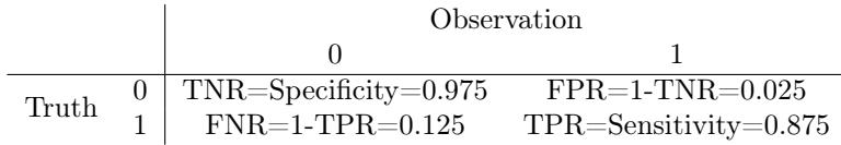
Table 2.1: Likelihood function p(Y |H) for a binary observation Y given two possible hidden states H. Each row sums to one. Abbreviations: TNR is true negative rate, TPR is true positive rate, FNR is false negative rate, FPR is false positive rate.

Normalizing the joint distribution by computing p(H = h, Y = y)/p(Y = y) for each h gives the posterior distribution p(H = h|Y = y); this represents our new belief state about the possible values of H.

We can summarize Bayes rule in words as follows:

posterior ∞ prior ↓ likelihood (2.54)

Here we use the symbol ∞ to denote “proportional to”, since we are ignoring the denominator, which is just a constant, independent of H. Using Bayes rule to update a distribution over unknown values of some quantity of interest, given relevant observed data, is called Bayesian inference, or posterior inference. It can also just be called probabilistic inference.

Below we give some simple examples of Bayesian inference in action. We will see many more interesting examples later in this book.

2.3.1 Example: Testing for COVID-19

Suppose you think you may have contracted COVID-19, which is an infectious disease caused by the SARS-CoV-2 virus. You decide to take a diagnostic test, and you want to use its result to determine if you are infected or not.

Let H = 1 be the event that you are infected, and H = 0 be the event you are not infected. Let Y = 1 if the test is positive, and Y = 0 if the test is negative. We want to compute p(H = h|Y = y), for h → {0, 1}, where y is the observed test outcome. (We will write the distribution of values, [p(H = 0|Y = y), p(H = 1|Y = y)] as p(H|y), for brevity.) We can think of this as a form of binary classification, where H is the unknown class label, and y is the feature vector.

First we must specify the likelihood. This quantity obviously depends on how reliable the test is. There are two key parameters. The sensitivity (aka true positive rate) is defined as p(Y = 1|H = 1), i.e., the probability of a positive test given that the truth is positive. The false negative rate is defined as one minus the sensitivity. The specificity (aka true negative rate) is defined as p(Y = 0|H = 0), i.e., the probability of a negative test given that the truth is negative. The false positive rate is defined as one minus the specificity. We summarize all these quantities in Table 2.1. (See Section 5.1.3.1 for more details.) Following https://nyti.ms/31MTZgV, we set the sensitivity to 87.5% and the specificity to 97.5%.

Next we must specify the prior. The quantity p(H = 1) represents the prevalence of the disease in the area in which you live. We set this to p(H = 1) = 0.1 (i.e., 10%), which was the prevalence in New York City in Spring 2020. (This example was chosen to match the numbers in https://nyti.ms/31MTZgV.)

Now suppose you test positive. We have

\[p(H=1|Y=1) = \frac{p(Y=1|H=1)p(H=1)}{p(Y=1|H=1)p(H=1) + p(Y=1|H=0)p(H=0)}\tag{2.55}\]

\[\eta = \frac{\text{TPR} \times \text{prior}}{\text{TPR} \times \text{prior} + \text{FPR} \times (1 - \text{prior})} \tag{2.56}\]

\[\eta = \frac{0.875 \times 0.1}{0.875 \times 0.1 + 0.025 \times 0.9} = 0.795\tag{2.57}\]

So there is a 79.5% chance you are infected.

Now suppose you test negative. The probability you are infected is given by

\[p(H=1|Y=0) = \frac{p(Y=0|H=1)p(H=1)}{p(Y=0|H=1)p(H=1) + p(Y=0|H=0)p(H=0)}\tag{2.58}\]

\[\eta = \frac{\text{FNR} \times \text{prior}}{\text{FNR} \times \text{prior} + \text{TNR} \times (1 - \text{prior})} \tag{2.59}\]

\[\eta = \frac{0.125 \times 0.1}{0.125 \times 0.1 + 0.975 \times 0.9} = 0.014\tag{2.60}\]

So there is just a 1.4% chance you are infected.

Nowadays COVID-19 prevalence is much lower. Suppose we repeat these calculations using a base rate of 1%; now the posteriors reduce to 26% and 0.13% respectively.

The fact that you only have a 26% chance of being infected with COVID-19, even after a positive test, is very counter-intuitive. The reason is that a single positive test is more likely to be a false positive than due to the disease, since the disease is rare. To see this, suppose we have a population of 100,000 people, of whom 1000 are infected. Of those who are infected, 875 = 0.875 ↓ 1000 test positive, and of those who are uninfected, 2475 = 0.025↓99, 000 test positive. Thus the total number of positives is 3350 = 875 + 2475, so the posterior probability of being infected given a positive test is 875/3350 = 0.26.

Of course, the above calculations assume we know the sensitivity and specificity of the test. See [GC20] for how to apply Bayes rule for diagnostic testing when there is uncertainty about these parameters.

2.3.2 Example: The Monty Hall problem

In this section, we consider a more “frivolous” application of Bayes rule. In particular, we apply it to the famous Monty Hall problem.

Imagine a game show with the following rules: There are three doors, labeled 1, 2, 3. A single prize (e.g., a car) has been hidden behind one of them. You get to select one door. Then the gameshow host opens one of the other two doors (not the one you picked), in such a way as to not reveal the prize location. At this point, you will be given a fresh choice of door: you can either stick with your first choice, or you can switch to the other closed door. All the doors will then be opened and you will receive whatever is behind your final choice of door.

For example, suppose you choose door 1, and the gameshow host opens door 3, revealing nothing behind the door, as promised. Should you (a) stick with door 1, or (b) switch to door 2, or (c) does it make no di!erence?

Door 1	Door 2	Door 3	Switch	Stay
Car	-	-	Lose	Win
-	Car	-	Win	Lose
-	-	Car	Win	Lose

Table 2.2: 3 possible states for the Monty Hall game, showing that switching doors is two times better (on average) than staying with your original choice. Adapted from Table 6.1 of [PM18].

Intuitively, it seems it should make no di!erence, since your initial choice of door cannot influence the location of the prize. However, the fact that the host opened door 3 tells us something about the location of the prize, since he made his choice conditioned on the knowledge of the true location and on your choice. As we show below, you are in fact twice as likely to win the prize if you switch to door 2.

To show this, we will use Bayes’ rule. Let Hⁱ denote the hypothesis that the prize is behind door i. We make the following assumptions: the three hypotheses H1, H² and H³ are equiprobable a priori, i.e.,

\[P(H\_1) = P(H\_2) = P(H\_3) = \frac{1}{3}.\tag{2.61}\]

The datum we receive, after choosing door 1, is either Y = 3 and Y = 2 (meaning door 3 or 2 is opened, respectively). We assume that these two possible outcomes have the following probabilities. If the prize is behind door 1, then the host selects at random between Y = 2 and Y = 3. Otherwise the choice of the host is forced and the probabilities are 0 and 1.

\[\begin{array}{|c|c|c|} \hline P(Y=2|H\_1)=\frac{1}{2} & P(Y=2|H\_2)=0 \\ P(Y=3|H\_1)=\frac{1}{2} & P(Y=3|H\_2)=1 \\ \hline \end{array}\left|\begin{array}{c}P(Y=2|H\_3)=1 \\ P(Y=3|H\_3)=0 \\ \hline \end{array}\right|\tag{2.62}\]

Now, using Bayes’ theorem, we evaluate the posterior probabilities of the hypotheses:

\[P(H\_i|Y=3) = \frac{P(Y=3|H\_i)P(H\_i)}{P(Y=3)}\tag{2.63}\]

\[\left\lfloor P(H\_1|Y=3) = \frac{(1/2)(1/3)}{P(Y=3)} \right\rfloor \left\lfloor P(H\_2|Y=3) = \frac{(1)(1/3)}{P(Y=3)} \right\rfloor \left\lfloor P(H\_3|Y=3) = \frac{(0)(1/3)}{P(Y=3)} \right\rfloor \tag{2.64}\]

The denominator P(Y = 3) is P(Y = 3) = ^{1 6 + 1 3 = 1 2} . So

\[\left| P(H\_1 | Y = 3) \right. \quad = \left. \frac{1}{3} \right| P(H\_2 | Y = 3) \quad = \left. \frac{2}{3} \right| P(H\_3 | Y = 3) \quad = \left. 0. \right| \tag{2.65}\]

So the contestant should switch to door 2 in order to have the biggest chance of getting the prize. See Table 2.2 for a worked example.

Many people find this outcome surprising. One way to make it more intuitive is to perform a thought experiment in which the game is played with a million doors. The rules are now that the contestant chooses one door, then the game show host opens 999,998 doors in such a way as not to reveal the prize, leaving the contestant’s selected door and one other door closed. The contestant may now stick or switch. Imagine the contestant confronted by a million doors, of which doors 1 and 234,598 have not been opened, door 1 having been the contestant’s initial guess. Where do you think the prize is?

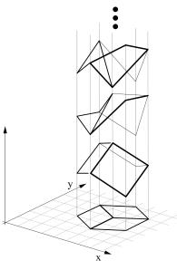
Figure 2.8: Any planar line-drawing is geometrically consistent with infinitely many 3-D structures. From Figure 11 of [SA93]. Used with kind permission of Pawan Sinha.

2.3.3 Inverse problems *

Probability theory is concerned with predicting a distribution over outcomes y given knowledge (or assumptions) about the state of the world, h. By contrast, inverse probability is concerned with inferring the state of the world from observations of outcomes. We can think of this as inverting the h ↔︎ y mapping.

For example, consider trying to infer a 3d shape h from a 2d image y, which is a classic problem in visual scene understanding. Unfortunately, this is a fundamentally ill-posed problem, as illustrated in Figure 2.8, since there are multiple possible hidden h’s consistent with the same observed y (see e.g., [Piz01]). Similarly, we can view natural language understanding as an ill-posed problem, in which the listener must infer the intention h from the (often ambiguous) words spoken by the speaker (see e.g., [Sab21]).

To tackle such inverse problems, we can use Bayes’ rule to compute the posterior, p(h|y), which gives a distribution over possible states of the world. This requires specifying the forwards model, p(y|h), as well as a prior p(h), which can be used to rule out (or downweight) implausible world states. We discuss this topic in more detail in the sequel to this book, [Mur23].

2.4 Bernoulli and binomial distributions

Perhaps the simplest probability distribution is the Bernoulli distribution, which can be used to model binary events, as we discuss below.

2.4.1 Definition

Consider tossing a coin, where the probability of event that it lands heads is given by 0 ↘ ϖ ↘ 1. Let Y = 1 denote this event, and let Y = 0 denote the event that the coin lands tails. Thus we are assuming that p(Y = 1) = ϖ and p(Y = 0) = 1 ↑ ϖ. This is called the Bernoulli distribution, and can be written as follows

\[Y \sim \text{Ber}(\theta) \tag{2.66}\]

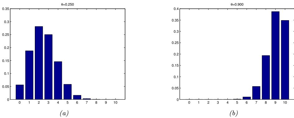
Figure 2.9: Illustration of the binomial distribution with N = 10 and (a) ε = 0.25 and (b) ε = 0.9. Generated by binom\_dist\_plot.ipynb.

where the symbol ⇒ means “is sampled from” or “is distributed as”, and Ber refers to Bernoulli. The probability mass function (pmf) of this distribution is defined as follows:

\[\text{Ber}(y|\theta) = \begin{cases} 1 - \theta & \text{if } y = 0 \\ \theta & \text{if } y = 1 \end{cases} \tag{2.67}\]

(See Section 2.2.1 for details on pmf’s.) We can write this in a more concise manner as follows:

\[\text{Ber}(y|\theta) \stackrel{\Delta}{=} \theta^y (1-\theta)^{1-y} \tag{2.68}\]

The Bernoulli distribution is a special case of the binomial distribution. To explain this, suppose we observe a set of N Bernoulli trials, denoted yⁿ ⇒ Ber(·|ϖ), for n =1: N. Concretely, think of tossing a coin N times. Let us define s to be the total number of heads, s ↭ $^{N n}=1 I(yⁿ = 1). The distribution of s is given by the binomial distribution:

\[\operatorname{Bin}(s|N,\theta) \triangleq \binom{N}{s} \theta^s (1-\theta)^{N-s} \tag{2.69}\]

where

\[ \binom{N}{k} \triangleq \frac{N!}{(N-k)!k!} \tag{2.70} \]

is the number of ways to choose k items from N (this is known as the binomial coe!cient, and is pronounced “N choose k”). See Figure 2.9 for some examples of the binomial distribution. If N = 1, the binomial distribution reduces to the Bernoulli distribution.

2.4.2 Sigmoid (logistic) function

When we want to predict a binary variable y → {0, 1} given some inputs x → X , we need to use a conditional probability distribution of the form

\[p(y|x,\theta) = \text{Ber}(y|f(x;\theta))\tag{2.71}\]

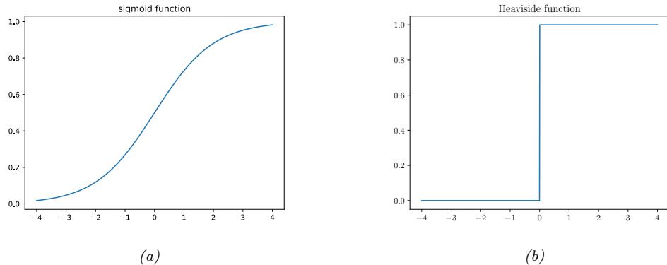
Figure 2.10: (a) The sigmoid (logistic) function ϑ(a) = (1 + e→^a) ^→1. (b) The Heaviside function I(a > 0). Generated by activation\_fun\_plot.ipynb.

\[ \sigma(x) \triangleq \frac{1}{1 + e^{-x}} = \frac{e^x}{1 + e^x} \tag{2.72} \]

\[ \frac{d}{dx}\sigma(x) = \sigma(x)(1 - \sigma(x)) \tag{2.73} \]

\[ 1 - \sigma(x) = \sigma(-x) \tag{2.74} \]

\[ \sigma^{-1}(p) = \log\left(\frac{p}{1 - p}\right) \triangleq \text{logit}(p) \tag{2.75} \]

\[ \sigma\_+(x) \triangleq \log(1 + e^x) \triangleq \text{softplus}(x) \tag{2.76} \]

\[ \frac{d}{dx}\sigma\_+(x) = \sigma(x) \tag{2.77} \]

Table 2.3: Some useful properties of the sigmoid (logistic) and related functions. Note that the logit function is the inverse of the sigmoid function, and has a domain of [0, 1].

where f(x; ω) is some function that predicts the mean parameter of the output distribution. We will consider many di!erent kinds of function f in Part II–Part IV.

To avoid the requirement that 0 ↘ f(x; ω) ↘ 1, we can let f be an unconstrained function, and use the following model:

\[p(y|x,\theta) = \text{Ber}(y|\sigma(f(x;\theta)))\tag{2.78}\]

Here ε() is the sigmoid or logistic function, defined as follows:

\[ \sigma(a) \stackrel{\Delta}{=} \frac{1}{1 + e^{-a}} \tag{2.79} \]

where a = f(x; ω). The term “sigmoid” means S-shaped: see Figure 2.10a for a plot. We see that it

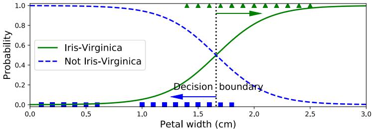
Figure 2.11: Logistic regression applied to a 1-dimensional, 2-class version of the Iris dataset. Generated by iris\_logreg.ipynb. Adapted from Figure 4.23 of [Gér19].

maps the whole real line to [0, 1], which is necessary for the output to be interpreted as a probability (and hence a valid value for the Bernoulli parameter ϖ). The sigmoid function can be thought of as a “soft” version of the heaviside step function, defined by

\[H(a) \triangleq \mathbb{I}(a > 0)\tag{2.80}\]

as shown in Figure 2.10b.

Plugging the definition of the sigmoid function into Equation (2.78) we get

\[p(y=1|x,\theta) = \frac{1}{1+e^{-a}} = \frac{e^a}{1+e^a} = \sigma(a) \tag{2.81}\]

\[p(y=0|x,\theta) = 1 - \frac{1}{1+e^{-a}} = \frac{e^{-a}}{1+e^{-a}} = \frac{1}{1+e^a} = \sigma(-a) \tag{2.82}\]

The quantity a is equal to the log odds, log( ^{p 1}→^p ), where ^{p = p}(^y = 1|x; ^ω). To see this, note that

\[\log\left(\frac{p}{1-p}\right) = \log\left(\frac{e^a}{1+e^a}\frac{1+e^a}{1}\right) = \log(e^a) = a\tag{2.83}\]

The logistic function or sigmoid function maps the log-odds a to p:

\[p = \text{logistic}(a) = \sigma(a) \stackrel{\Delta}{=} \frac{1}{1 + e^{-a}} = \frac{e^a}{1 + e^a} \tag{2.84}\]

The inverse of this is called the logit function, and maps p to the log-odds a:

\[a = \text{logit}(p) = \sigma^{-1}(p) \triangleq \log\left(\frac{p}{1-p}\right) \tag{2.85}\]

See Table 2.3 for some useful properties of these functions.

2.4.3 Binary logistic regression

In this section, we use a conditional Bernoulli model, where we use a linear predictor of the form f(x; ω) = w^Tx + b. Thus the model has the form

\[p(y|x; \theta) = \text{Ber}(y|\sigma(w^\mathsf{T}x + b))\tag{2.86}\]

In other words,

\[p(y=1|x; \theta) = \sigma(w^\top x + b) = \frac{1}{1 + e^{-(w^\top x + b)}}\tag{2.87}\]

This is called logistic regression.

For example consider a 1-dimensional, 2-class version of the iris dataset, where the positive class is “Virginica” and the negative class is “not Virginica”, and the feature x we use is the petal width. We fit a logistic regression model to this and show the results in Figure 2.11. The decision boundary corresponds to the value x^↓ where p(y = 1|x = x↓, ω)=0.5. We see that, in this example, x^↓ ↖ 1.7. As x moves away from this boundary, the classifier becomes more confident in its prediction about the class label.

It should be clear from this example why it would be inappropriate to use linear regression for a (binary) classification problem. In such a model, the probabilities would increase above 1 as we move far enough to the right, and below 0 as we move far enough to the left.

For more detail on logistic regression, see Chapter 10.

2.5 Categorical and multinomial distributions

To represent a distribution over a finite set of labels, y → {1,…,C}, we can use the categorical distribution, which generalizes the Bernoulli to C > 2 values.

2.5.1 Definition

The categorical distribution is a discrete probability distribution with one parameter per class:

\[\text{Cat}(y|\theta) \stackrel{\Delta}{=} \prod\_{c=1}^{C} \theta\_c^{l(y=c)} \tag{2.88}\]

In other words, p(y = c|ω) = ϖc. Note that the parameters are constrained so that 0 ↘ ϖ^c ↘ 1 and $^{C c}=1 ϖ^c = 1; thus there are only C ↑ 1 independent parameters.

We can write the categorical distribution in another way by converting the discrete variable y into a one-hot vector with C elements, all of which are 0 except for the entry corresponding to the class label. (The term “one-hot” arises from electrical engineering, where binary vectors are encoded as electrical current on a set of wires, which can be active (“hot”) or not (“cold”).) For example, if C = 3, we encode the classes 1, 2 and 3 as (1, 0, 0), (0, 1, 0), and (0, 0, 1). More generally, we can encode the classes using unit vectors, where e^c is all 0s except for dimension c. (This is also called a dummy encoding.) Using one-hot encodings, we can write the categorical distribution as follows:

\[\text{Cat}(y|\theta) \stackrel{\Delta}{=} \prod\_{c=1}^{C} \theta\_c^{y\_c} \tag{2.89}\]

The categorical distribution is a special case of the multinomial distribution. To explain this, suppose we observe N categorical trials, yⁿ ⇒ Cat(·|ω), for n =1: N. Concretely, think of rolling a C-sided dice N times. Let us define y to be a vector that counts the number of times each face

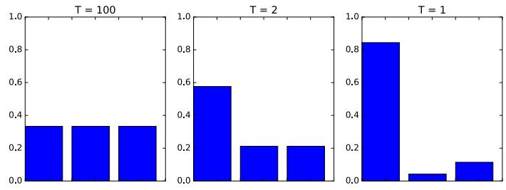
Figure 2.12: Softmax distribution softmax(a/T), where a = (3, 0, 1), at temperatures of T = 100, T = 2 and T = 1. When the temperature is high (left), the distribution is uniform, whereas when the temperature is low (right), the distribution is “spiky”, with most of its mass on the largest element. Generated by softmax\_plot.ipynb.

shows up, i.e., y^c = N^c ↭ $^{N n}=1 I(yⁿ = c). Now y is no longer one-hot, but is “multi-hot”, since it has a non-zero entry for every value of c that was observed across all N trials. The distribution of y is given by the multinomial distribution:

\[\mathcal{M}(\boldsymbol{y}|N,\boldsymbol{\theta}) \triangleq \binom{N}{y\_1 \dots y\_C} \prod\_{c=1}^C \theta\_c^{y\_c} = \binom{N}{N\_1 \dots N\_C} \prod\_{c=1}^C \theta\_c^{N\_c} \tag{2.90}\]

where ϖ^c is the probability that side c shows up, and

\[\binom{N}{N\_1\dots N\_C} \stackrel{\Delta}{=} \frac{N!}{N\_1! N\_2! \cdots N\_C!} \tag{2.91}\]

is the multinomial coe!cient, which is the number of ways to divide a set of size N = $^{C c}=1 N^c into subsets with sizes N¹ up to N^C . If N = 1, the multinomial distribution becomes the categorical distribution.

2.5.2 Softmax function

In the conditional case, we can define

\[p(y|x,\theta) = \text{Cat}(y|f(x;\theta))\tag{2.92}\]

which we can also write as

\[p(y|x,\theta) = \mathcal{M}(y|1, f(x;\theta))\tag{2.93}\]

We require that ⁰ ↘ ^fc(x; ^ω) ↘ ¹ and $^{C c}=1 fc(x; ω)=1.

To avoid the requirement that f directly predict a probability vector, it is common to pass the output from f into the softmax function [Bri90], also called the multinomial logit. This is defined as follows:

\[\text{softmax}(\mathbf{a}) \triangleq \left[ \frac{e^{a\_1}}{\sum\_{c'=1}^C e^{a\_{c'}}}, \dots, \frac{e^{a\_C}}{\sum\_{c'=1}^C e^{a\_{c'}}} \right] \tag{2.94}\]

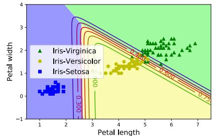
Figure 2.13: Logistic regression on the 3-class, 2-feature version of the Iris dataset. Adapted from Figure of 4.25 [Gér19]. Generated by iris\_logreg.ipynb.

This maps ^RC to [0, 1]^C , and satisfies the constraints that ⁰ ↘ softmax(a)^c ↘ ¹ and $^{C c}=1 softmax(a)^c = 1. The inputs to the softmax, a = f(x; ω), are called logits, and are a generalization of the log odds.

The softmax function is so-called since it acts a bit like the argmax function. To see this, let us divide each a^c by a constant T called the temperature. 8 Then as ^{T ↔︎ 0}, we find

\[\text{softmax}(\mathbf{a}/T)\_c = \begin{cases} 1.0 & \text{if } c = \text{argmax}\_{c'} a\_{c'} \\ 0.0 & \text{otherwise} \end{cases} \tag{2.95}\]

In other words, at low temperatures, the distribution puts most of its probability mass in the most probable state (this is called winner takes all), whereas at high temperatures, it spreads the mass uniformly. See Figure 2.12 for an illustration.

2.5.3 Multiclass logistic regression

If we use a linear predictor of the form f(x; ω) = Wx + b, where W is a C ↓ D matrix, and b is a C-dimensional bias vector, the final model becomes

\[p(y|x; \theta) = \text{Cat}(y|\text{softmax}(\mathbf{W}x + \mathbf{b})) \tag{2.96}\]

Let a = Wx + b be the C-dimensional vector of logits. Then we can rewrite the above as follows:

\[p(y=c|\mathbf{x}; \boldsymbol{\theta}) = \frac{e^{a\_c}}{\sum\_{c'=1}^{C} e^{a\_{c'}}} \tag{2.97}\]

This is known as multinomial logistic regression.

If we have just two classes, this reduces to binary logistic regression. To see this, note that

\[\text{softmax}(\mathbf{a})\_0 = \frac{e^{a\_0}}{e^{a\_0} + e^{a\_1}} = \frac{1}{1 + e^{a\_1 - a\_0}} = \sigma(a\_0 - a\_1) \tag{2.98}\]

so we can just train the model to predict a = a¹ ↑ a0. This can be done with a single weight vector w; if we use the multi-class formulation, we will have two weight vectors, w⁰ and w1. Such a model is over-parameterized, which can hurt interpretability, but the predictions will be the same.

^8. This terminology comes from the area of statistical physics. The Boltzmann distribution is a distribution over states which has the same form as the softmax function.

We discuss this in more detail in Section 10.3. For now, we just give an example. Figure 2.13 shows what happens when we fit this model to the 3-class iris dataset, using just 2 features. We see that the decision boundaries between each class are linear. We can create nonlinear boundaries by transforming the features (e.g., using polynomials), as we discuss in Section 10.3.1.

2.5.4 Log-sum-exp trick

In this section, we discuss one important practical detail to pay attention to when working with the softmax distribution. Suppose we want to compute the normalized probability p^c = p(y = c|x), which is given by

\[p\_c = \frac{e^{a\_c}}{Z(\mathbf{a})} = \frac{e^{a\_c}}{\sum\_{c'=1}^C e^{a\_{c'}}}\tag{2.99}\]

where a = f(x; ω) are the logits. We might encounter numerical problems when computing the partition function Z. For example, suppose we have 3 classes, with logits a = (0, 1, 0). Then we find ^{Z = e0}+e¹+e⁰ = 4.71. But now suppose ^a = (1000, ¹⁰⁰¹, 1000); we find ^{Z = ∈}, since on a computer, even using 64 bit precision, np.exp(1000)=inf. Similarly, suppose a = (↑1000, ↑999, ↑1000); now we find Z = 0, since np.exp(-1000)=0. To avoid numerical problems, we can use the following identity:

\[\log \sum\_{c=1}^{C} \exp(a\_c) = m + \log \sum\_{c=1}^{C} \exp(a\_c - m) \tag{2.100}\]

This holds for any m. It is common to use m = max^c a^c which ensures that the largest value you exponentiate will be zero, so you will definitely not overflow, and even if you underflow, the answer will be sensible. This is known as the log-sum-exp trick. We use this trick when implementing the lse function:

\[\text{lse}(\mathbf{a}) \triangleq \log \sum\_{c=1}^{C} \exp(a\_c) \tag{2.101}\]

We can use this to compute the probabilities from the logits:

\[p(y=c|\mathbf{z}) = \exp(a\_c - \text{lse}(\mathbf{a})) \tag{2.102}\]

We can then pass this to the cross-entropy loss, defined in Equation (5.41).

However, to save computational e!ort, and for numerical stability, it is quite common to modify the cross-entropy loss so that it takes the logits a as inputs, instead of the probability vector p. For example, consider the binary case. The CE loss for one example is

\[\mathcal{L} = -\left[\mathbb{I}\left(y = 0\right)\log p\_0 + \mathbb{I}\left(y = 1\right)\log p\_1\right] \tag{2.103}\]

where

\[\log p\_1 = \log \left(\frac{1}{1 + \exp(-a)}\right) = \log(1) - \log(1 + \exp(-a)) = 0 - \text{lse}([0, -a]) \tag{2.104}\]

\[\log p\_0 = 0 - \text{lse}([0, +a]) \tag{2.105}\]

2.6 Univariate Gaussian (normal) distribution

The most widely used distribution of real-valued random variables y → R is the Gaussian distribution, also called the normal distribution (see Section 2.6.4 for a discussion of these names).

2.6.1 Cumulative distribution function

We define the cumulative distribution function or cdf of a continuous random variable Y as follows:

\[P(y) \triangleq \Pr(Y \le y) \tag{2.106}\]

(Note that we use a capital P to represent the cdf.) Using this, we can compute the probability of being in any interval as follows:

\[\Pr(a < Y \le b) = P(b) - P(a) \tag{2.107}\]

Cdf’s are monotonically non-decreasing functions.

The cdf of the Gaussian is defined by

\[\Phi(y;\mu,\sigma^2) \triangleq \int\_{-\infty}^{y} \mathcal{N}(z|\mu,\sigma^2) dz \tag{2.108}\]

See Figure 2.2a for a plot. Note that the cdf of the Gaussian is often implemented using !(y; µ, ε²) = 1 ² [1 + erf(z/≃2)], where ^z = (^{y ↑ µ})/^ε and erf(u) is the error function, defined as

\[\text{erf}(u) \triangleq \frac{2}{\sqrt{\pi}} \int\_0^u e^{-t^2} dt\tag{2.109}\]

The parameter µ encodes the mean of the distribution; in the case of a Gaussian, this is also the same as the mode. The parameter ε² encodes the variance. (Sometimes we talk about the precision of a Gaussian, which is the inverse variance, denoted φ = 1/ε².) When µ = 0 and ε = 1, the Gaussian is called the standard normal distribution.

If ^P is the cdf of ^Y , then ^{P →1}(q) is the value ^yq such that ^p(^Y ↘ ^yq) = ^q; this is called the ^q’th quantile of P. The value P ^→1(0.5) is the median of the distribution, with half of the probability mass on the left, and half on the right. The values P ^→1(0.25) and P ^→1(0.75) are the lower and upper quartiles.

For example, let ! be the cdf of the Gaussian distribution ^N (0, 1), and !→¹ be the inverse cdf (also known as the probit function). Then points to the left of !→1(ϱ/2) contain ϱ/2 of the probability mass, as illustrated in Figure 2.2b. By symmetry, points to the right of !→¹(1 ^{↑ ϱ}/2) also contain ^ϱ/² of the mass. Hence the central interval (!→1(ϱ/2), !→1(1 ^{↑ ϱ}/2)) contains ^{1 ↑ ϱ} of the mass. If we set ϱ = 0.05, the central 95% interval is covered by the range

\[(\Phi^{-1}(0.025), \Phi^{-1}(0.975)) = (-1.96, 1.96) \tag{2.110}\]

If the distribution is ^N (µ, ^ε2), then the 95% interval becomes (^{µ ↑ 1}.96ε, µ + 1.96ε). This is often approximated by writing µ ± 2ε.

2.6.2 Probability density function

We define the probability density function or pdf as the derivative of the cdf:

\[p(y) \triangleq \frac{d}{dy}P(y) \tag{2.111}\]

The pdf of the Gaussian is given by

\[\mathcal{N}(y|\mu,\sigma^2) \triangleq \frac{1}{\sqrt{2\pi\sigma^2}} e^{-\frac{1}{2\sigma^2}(y-\mu)^2} = \phi(y;\mu,\sigma^2) \tag{2.112}\]

where ^≃ 2ϑε² is the normalization constant needed to ensure the density integrates to 1 (see Exercise 2.12). See Figure 2.2b for a plot. (If µ = 0 and ε = 1, this is called the standard normal, and the density is denoted by ↼(y).)

Given a pdf, we can compute the probability of a continuous variable being in a finite interval as follows:

\[\Pr(a < Y \le b) = \int\_{a}^{b} p(y) dy = P(b) - P(a) \tag{2.113}\]

As the size of the interval gets smaller, we can write

\[\Pr(y \le Y \le y + dy) \approx p(y)dy\tag{2.114}\]

Intuitively, this says the probability of Y being in a small interval around y is the density at y times the width of the interval. One important consequence of the above result is that the pdf at a point can be larger than 1. For example, N (0|0, 0.1) = 3.99.

We can use the pdf to compute the mean, or expected value, of the distribution:

\[\mathbb{E}\left[Y\right] \stackrel{\Delta}{=} \int\_{\mathcal{Y}} y \, p(y) dy\tag{2.115}\]

For a Gaussian, we have the familiar result that E + ^N (·|µ, ^ε2) , = µ. (Note, however, that for some distributions, this integral is not finite, so the mean is not defined.)

We can also use the pdf to compute the variance of a distribution. This is a measure of the “spread”, and is often denoted by ε². The variance is defined as follows:

\[\mathbb{E}\left[Y\right] \stackrel{\Delta}{=} \mathbb{E}\left[\left(Y-\mu\right)^{2}\right] = \int (y-\mu)^{2}p(y)dy\tag{2.116}\]

\[I = \int y^2 p(y) dy + \mu^2 \int p(y) dy - 2\mu \int yp(y) dy = \mathbb{E} \left[ Y^2 \right] - \mu^2 \tag{2.117}\]

from which we derive the useful result

\[\mathbb{E}\left[Y^2\right] = \sigma^2 + \mu^2\tag{2.118}\]

The standard deviation is defined as

\[\text{std}\left[Y\right] \stackrel{\Delta}{=} \sqrt{\mathbb{V}\left[Y\right]} = \sigma\]

(The standard deviation can be more intepretable than the variance since it has the same units as Y itself.) For a Gaussian, we have the familiar result that std + ^N (·|µ, ^ε2) , = ε.

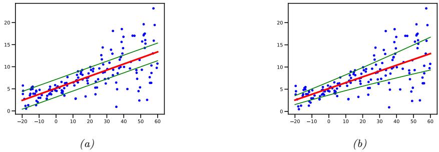
Figure 2.14: Linear regression using Gaussian output with mean µ(x) = b + wx and (a) fixed variance ϑ² (homoskedastic) or (b) input-dependent variance ϑ(x) ² (heteroscedastic). Generated by linreg\_1d\_hetero\_tfp.ipynb.

2.6.3 Regression

So far we have been considering the unconditional Gaussian distribution. In some cases, it is helpful to make the parameters of the Gaussian be functions of some input variables, i.e., we want to create a conditional density model of the form

\[p(y|x; \theta) = \mathcal{N}(y|f\_{\mu}(x; \theta), f\_{\sigma}(x; \theta)^2) \tag{2.120}\]

where ^fµ(x; ^ω) ^{→ R} predicts the mean, and ^fε(x; ^ω)^{2 → R+} predicts the variance.

It is common to assume that the variance is fixed, and is independent of the input. This is called homoscedastic regression. Furthermore it is common to assume the mean is a linear function of the input. The resulting model is called linear regression:

\[p(y|\mathbf{z}; \boldsymbol{\theta}) = \mathcal{N}(y|\mathbf{w}^\mathsf{T}\mathbf{z} + b, \sigma^2) \tag{2.121}\]

where ω = (w, b, ε²). See Figure 2.14(a) for an illustration of this model in 1d. and Section 11.2 for more details on this model.

However, we can also make the variance depend on the input; this is called heteroskedastic regression. In the linear regression setting, we have

\[p(y|x; \boldsymbol{\theta}) = \mathcal{N}(y|w\_{\mu}^{\mathsf{T}}x + b, \sigma\_{+}(w\_{\sigma}^{\mathsf{T}}x)) \tag{2.122}\]

where ω = (wµ, wε) are the two forms of regression weights, and

\[ \sigma\_+(a) = \log(1 + e^a) \tag{2.123} \]

is the softplus function, that maps from R to R+, to ensure the predicted standard deviation is non-negative. See Figure 2.14(b) for an illustration of this model in 1d.

Note that Figure 2.14 plots the 95% predictive interval, [µ(x) ↑ 2ε(x), µ(x)+2ε(x)]. This is the uncertainty in the predicted observation y given x, and captures the variability in the blue dots. By contrast, the uncertainty in the underlying (noise-free) function is represented by -V [fµ(x; ω)], which does not involve the ε term; now the uncertainty is over the parameters ω, rather than the output y. See Section 11.7 for details on how to model parameter uncertainty.

2.6.4 Why is the Gaussian distribution so widely used?

The Gaussian distribution is the most widely used distribution in statistics and machine learning. There are several reasons for this. First, it has two parameters which are easy to interpret, and which capture some of the most basic properties of a distribution, namely its mean and variance. Second, the central limit theorem (Section 2.8.6) tells us that sums of independent random variables have an approximately Gaussian distribution, making it a good choice for modeling residual errors or “noise”. Third, the Gaussian distribution makes the least number of assumptions (has maximum entropy), subject to the constraint of having a specified mean and variance, as we show in Section 3.4.4; this makes it a good default choice in many cases. Finally, it has a simple mathematical form, which results in easy to implement, but often highly e!ective, methods, as we will see in Section 3.2.

From a historical perspective, it’s worth remarking that the term “Gaussian distribution” is a bit misleading, since, as Jaynes [Jay03, p241] notes: “The fundamental nature of this distribution and its main properties were noted by Laplace when Gauss was six years old; and the distribution itself had been found by de Moivre before Laplace was born”. However, Gauss popularized the use of the distribution in the 1800s, and the term “Gaussian” is now widely used in science and engineering.

The name “normal distribution” seems to have arisen in connection with the normal equations in linear regression (see Section 11.2.2.2). However, we prefer to avoid the term “normal”, since it suggests other distributions are “abnormal”, whereas, as Jaynes [Jay03] points out, it is the Gaussian that is abnormal in the sense that it has many special properties that are untypical of general distributions.

2.6.5 Dirac delta function as a limiting case

As the variance of a Gaussian goes to 0, the distribution approaches an infinitely narrow, but infinitely tall, “spike” at the mean. We can write this as follows:

\[\lim\_{\sigma \to 0} \mathcal{N}(y|\mu, \sigma^2) \to \delta(y - \mu) \tag{2.124}\]

where ↽ is the Dirac delta function, defined by

\[\delta(x) = \begin{cases} +\infty & \text{if } x = 0 \\ 0 & \text{if } x \neq 0 \end{cases} \tag{2.125}\]

where

\[\int\_{-\infty}^{\infty} \delta(x) dx = 1\]

A slight variant of this is to define

\[\delta\_y(x) = \begin{cases} +\infty & \text{if } x = y \\ 0 & \text{if } x \neq y \end{cases} \tag{2.127}\]

Note that we have

\[ \delta\_y(x) = \delta(x - y) \tag{2.128} \]

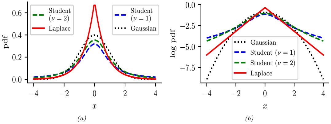
Figure 2.15: (a) The pdf ’s for a N (0, 1), T (µ = 0, ϑ = 1, ϖ = 1), T (µ = 0, ϑ = 1, ϖ = 2), and Laplace(0, 1/ ^↔︎2). The mean is 0 and the variance is 1 for both the Gaussian and Laplace. When ^ϖ = 1, the Student is the same as the Cauchy, which does not have a well-defined mean and variance. (b) Log of these pdf ’s. Note that the Student distribution is not log-concave for any parameter value, unlike the Laplace distribution. Nevertheless, both are unimodal. Generated by student\_laplace\_pdf\_plot.ipynb.

The delta function distribution satisfies the following sifting property, which we will use later on:

\[\int\_{-\infty}^{\infty} f(y)\delta(x-y)dy = f(x) \tag{2.129}\]

2.6.6 Truncated Gaussian distribution

Sometimes it is useful to restrict the Gaussian so it has support over a fixed interval, (a, b). This can be done by normalizing the Gaussian over this interval, giving rise to the truncated Gaussian:

\[\mathcal{N}(x|\mu,\sigma^2,a,b) = \frac{\frac{1}{\sigma}\phi(\frac{x-\mu}{\sigma})}{\Phi(\frac{b-\mu}{\sigma}) - \Phi(\frac{a-\mu}{\sigma})} \mathbb{I}\left(a < x < b\right)\]

For example, if a = 0, we restrict support to positive reals.

2.7 Some other common univariate distributions *

In this section, we briefly introduce some other univariate distributions that we will use in this book.

2.7.1 Student t distribution

The Gaussian distribution is quite sensitive to outliers. A robust alternative to the Gaussian is the Student t-distribution, which we shall call the Student distribution for short.9 Its pdf is as

^9. This distribution has a colorful etymology. It was first published in 1908 by William Sealy Gosset, who worked at the Guinness brewery in Dublin, Ireland. Since his employer would not allow him to use his own name, he called it the

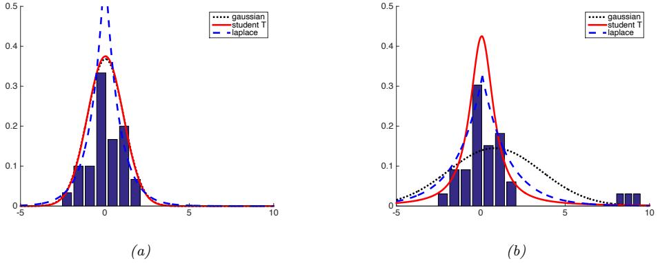
Figure 2.16: Illustration of the e!ect of outliers on fitting Gaussian, Student and Laplace distributions. (a) No outliers (the Gaussian and Student curves are on top of each other). (b) With outliers. We see that the Gaussian is more a!ected by outliers than the Student and Laplace distributions. Adapted from Figure 2.16 of [Bis06]. Generated by robust\_pdf\_plot.ipynb.

follows:

\[\mathcal{T}(y|\mu, \sigma^2, \nu) \propto \left[1 + \frac{1}{\nu} \left(\frac{y-\mu}{\sigma}\right)^2\right]^{-\left(\frac{\nu+1}{2}\right)}\tag{2.130}\]

where µ is the mean, ε > 0 is the scale parameter (not the standard deviation), and ⇀ > 0 is called the degrees of freedom (although a better term would be the degree of normality [Kru13], since large values of ⇀ make the distribution act like a Gaussian).

We see that the probability density decays as a polynomial function of the squared distance from the center, as opposed to an exponential function, so there is more probability mass in the tail than with a Gaussian distribution, as shown in Figure 2.15. We say that the Student distribution has heavy tails, which makes it robust to outliers.

To illustrate the robustness of the Student distribution, consider Figure 2.16. On the left, we show a Gaussian and a Student distribution fit to some data with no outliers. On the right, we add some outliers. We see that the Gaussian is a!ected a lot, whereas the Student hardly changes. We discuss how to use the Student distribution for robust linear regression in Section 11.6.2.

For later reference, we note that the Student distribution has the following properties:

\[\text{mean} = \mu, \text{ mode} = \mu, \text{ var} = \frac{\nu \sigma^2}{(\nu - 2)} \tag{2.131}\]

The mean is only defined if ⇀ > 1. The variance is only defined if ⇀ > 2. For ⇀ ⇐ 5, the Student distribution rapidly approaches a Gaussian distribution and loses its robustness properties. It is common to use ⇀ = 4, which gives good performance in a range of problems [LLT89].

^&quot;Student” distribution. The origin of the term t seems to have arisen in the context of tables of the Student distribution, used by Fisher when developing the basis of classical statistical inference. See http://jeff560.tripod.com/s.html for more historical details.

2.7.2 Cauchy distribution

If ⇀ = 1, the Student distribution is known as the Cauchy or Lorentz distribution. Its pdf is defined by

\[\mathcal{L}\left(x|\mu,\gamma\right) = \frac{1}{\gamma\pi} \left[1 + \left(\frac{x-\mu}{\gamma}\right)^2\right]^{-1} \tag{2.132}\]

This distribution has very heavy tails compared to a Gaussian. For example, 95% of the values from a standard normal are between -1.96 and 1.96, but for a standard Cauchy they are between -12.7 and 12.7. In fact the tails are so heavy that the integral that defines the mean does not converge.

The half Cauchy distribution is a version of the Cauchy (with µ = 0) that is “folded over” on itself, so all its probability density is on the positive reals. Thus it has the form

\[\mathcal{C}\_{+}(x|\gamma) \stackrel{\Delta}{=} \frac{2}{\pi \gamma} \left[ 1 + \left( \frac{x}{\gamma} \right)^{2} \right]^{-1} \tag{2.133}\]

This is useful in Bayesian modeling, where we want to use a distribution over positive reals with heavy tails, but finite density at the origin.

2.7.3 Laplace distribution

Another distribution with heavy tails is the Laplace distribution10, also known as the double sided exponential distribution. This has the following pdf:

\[\text{Laplace}(y|\mu, b) \stackrel{\Delta}{=} \frac{1}{2b} \exp\left(-\frac{|y-\mu|}{b}\right) \tag{2.134}\]

See Figure 2.15 for a plot. Here µ is a location parameter and b > 0 is a scale parameter. This distribution has the following properties:

\[\text{mean} = \mu, \text{ mode} = \mu, \text{ var} = 2b^2 \tag{2.135}\]

In Section 11.6.1, we discuss how to use the Laplace distribution for robust linear regression, and in Section 11.4, we discuss how to use the Laplace distribution for sparse linear regression.

2.7.4 Beta distribution

The beta distribution has support over the interval [0, 1] and its pdf is defined as follows:

\[\text{Beta}(x|a,b) = \frac{1}{B(a,b)} x^{a-1} (1-x)^{b-1} \tag{2.136}\]

where B(a, b) is the beta function, defined by

\[B(a,b) \triangleq \frac{\Gamma(a)\Gamma(b)}{\Gamma(a+b)}\tag{2.137}\]

^10. Pierre-Simon Laplace (1749–1827) was a French mathematician, who played a key role in creating the field of Bayesian statistics.

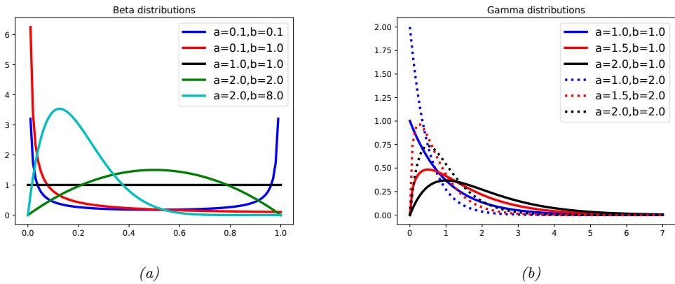
Figure 2.17: (a) Some beta distributions. If a < 1, we get a “spike” on the left, and if b < 1, we get a “spike” on the right. if a = b = 1, the distribution is uniform. If a > 1 and b > 1, the distribution is unimodal. Generated by beta\_dist\_plot.ipynb. (b) Some gamma distributions. If a ↗ 1, the mode is at 0, otherwise the mode is away from 0. As we increase the rate b, we reduce the horizontal scale, thus squeezing everything leftwards and upwards. Generated by gamma\_dist\_plot.ipynb.

where “(a) is the Gamma function defined by

\[ \Gamma(a) \stackrel{\Delta}{=} \int\_0^\infty x^{a-1} e^{-x} dx \tag{2.138} \]

See Figure 2.17a for plots of some beta distributions.

We require a, b > 0 to ensure the density is integrable (i.e., to ensure B(a, b) exists). If a = b = 1, we get the uniform distribution. If a and b are both less than 1, we get a bimodal distribution with “spikes” at 0 and 1; if a and b are both greater than 1, the distribution is unimodal.

For later reference, we note that the distribution has the following properties (Exercise 2.8):

\[\text{mean} = \frac{a}{a+b}, \text{ mode } = \frac{a-1}{a+b-2}, \text{ var} = \frac{ab}{(a+b)^2(a+b+1)}\tag{2.139}\]

Note that the above equation for the mode assumes a > 1 and b > 1; if a < 1 and b ∋ 1, the mode is at 0, and if a ∋ 1 and b < 1, the mode is at 1.

2.7.5 Gamma distribution

The gamma distribution is a flexible distribution for positive real valued rv’s, x > 0. It is defined in terms of two parameters, called the shape a > 0 and the rate b > 0. Its pdf is given by

\[\text{Ga}(x|\text{shape}=a, \text{rate}=b) \triangleq \frac{b^a}{\Gamma(a)} x^{a-1} e^{-xb} \tag{2.140}\]

Sometimes the distribution is parameterized in terms of the shape a and the scale s = 1/b:

\[\text{Ga}(x|\text{shape}=a,\text{scale}=s) \triangleq \frac{1}{s^a \Gamma(a)} x^{a-1} e^{-x/s} \tag{2.141}\]

See Figure 2.17b for some plots of the gamma pdf.

For reference, we note that the distribution has the following properties:

\[\text{mean} = \frac{a}{b}, \text{ mode} = \max(\frac{a-1}{b}, 0), \text{ var} = \frac{a}{b^2} \tag{2.142}\]

There are several distributions which are just special cases of the Gamma, which we discuss below.

• Exponential distribution. This is defined by

\[\text{Expon}(x|\lambda) \triangleq \text{Ga}(x|\text{shape}=1, \text{rate}=\lambda) \tag{2.143}\]

This distribution describes the times between events in a Poisson process, i.e. a process in which events occur continuously and independently at a constant average rate φ.

• Chi-squared distribution. This is defined by

\[ \chi^2\_\nu(x) \triangleq \text{Ga}(x|\text{shape}=\frac{\nu}{2}, \text{rate}=\frac{1}{2})\tag{2.144} \]

where ⇀ is called the degrees of freedom. This is the distribution of the sum of squared Gaussian random variables. More precisely, if ^{Zi ⇒ N} (0, 1), and ^{S =} $^{ϑ i}=1 Z^{2 i} , then ^{S ⇒ χ2} ϑ.

• The inverse Gamma distribution is defined as follows:

\[\text{IG}(x|\text{shape}=a,\text{scale}=b) \stackrel{\Delta}{=} \frac{b^a}{\Gamma(a)} x^{-(a+1)} e^{-b/x} \tag{2.145}\]

The distribution has these properties

\[\text{mean} = \frac{b}{a-1}, \text{mode} = \frac{b}{a+1}, \text{var} = \frac{b^2}{(a-1)^2(a-2)}\tag{2.146}\]

The mean only exists if a > 1. The variance only exists if a > 2. Note: if X ⇒ Ga(shape = a,rate = b), then 1/X ⇒ IG(shape = a,scale = b). (Note that b plays two di!erent roles in this case.)

2.7.6 Empirical distribution

Suppose we have a set of ^N samples ^{D =} {x(1),…,x(N) }, derived from a distribution p(X), where X → R. We can approximate the pdf using a set of delta functions (Section 2.6.5) or “spikes”, centered on these samples:

\[\hat{p}\_N(x) = \frac{1}{N} \sum\_{n=1}^N \delta\_{x^{(n)}}(x) \tag{2.147}\]

This is called the empirical distribution of the dataset D. An example of this, with N = 5, is shown in Figure 2.18(a).

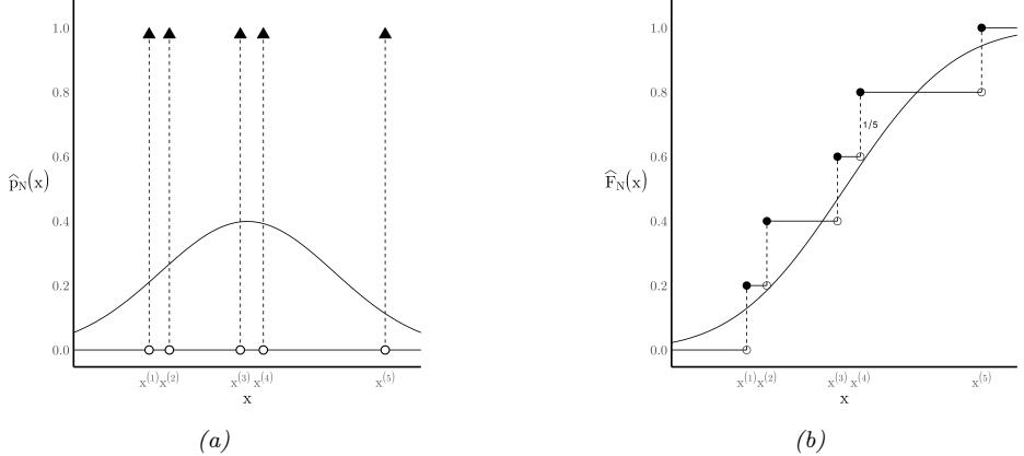
Figure 2.18: Illustration of the (a) empirical pdf and (b) empirical cdf derived from a set of N = 5 samples. From https: // bit. ly/ 3hFgi0e . Used with kind permission of Mauro Escudero.

The corresponding cdf is given by

\[\hat{P}\_N(x) = \frac{1}{N} \sum\_{n=1}^N \mathbb{I}\left(x^{(n)} \le x\right) = \frac{1}{N} \sum\_{n=1}^N u\_{x^{(n)}}(x) \tag{2.148}\]

where uy(x) is a step function at y defined by

\[u\_y(x) = \begin{cases} 1 & \text{if } x \ge y \\ 0 & \text{if } x < y \end{cases} \tag{2.149}\]

This can be visualized as a “stair case”, as in Figure 2.18(b), where the jumps of height 1/N occur at every sample.

2.8 Transformations of random variables *

Suppose x ⇒ p() is some random variable, and y = f(x) is some deterministic transformation of it. In this section, we discuss how to compute p(y).

2.8.1 Discrete case

If X is a discrete rv, we can derive the pmf for Y by simply summing up the probability mass for all the x’s such that f(x) = y:

\[p\_y(y) = \sum\_{x:f(x) = y} p\_x(x) \tag{2.150}\]

For example, if f(X)=1 if X is even and f(X)=0 otherwise, and px(X) is uniform on the set {1,…, ¹⁰}, then ^py(1) = $ ^x↑{2,4,6,8,10} ^px(x)=0.5, and hence ^py(0) = 0.5 also. Note that in this example, f is a many-to-one function.

2.8.2 Continuous case

If X is continuous, we cannot use Equation (2.150) since px(x) is a density, not a pmf, and we cannot sum up densities. Instead, we work with cdf’s, as follows:

\[P\_y(y) \stackrel{\Delta}{=} \Pr(Y \le y) = \Pr(f(X) \le y) = \Pr(X \in \{x | f(x) \le y\}) \tag{2.151}\]

If f is invertible, we can derive the pdf of y by di!erentiating the cdf, as we show below. If f is not invertible, we can use numerical integration, or a Monte Carlo approximation.

2.8.3 Invertible transformations (bijections)

In this section, we consider the case of monotonic and hence invertible functions. (Note a function is invertible i! it is a bijector). With this assumption, there is a simple formula for the pdf of y, as we will see. (This can be generalized to invertible, but non-monotonic, functions, but we ignore this case.)

2.8.3.1 Change of variables: scalar case

We start with an example. Suppose x ⇒ Unif(0, 1), and y = f(x)=2x + 1. This function stretches and shifts the probability distribution, as shown in Figure 2.19(a). Now let us zoom in on a point x and another point that is infinitesimally close, namely x + dx. We see this interval gets mapped to (y, y + dy). The probability mass in these intervals must be the same, hence p(x)dx = p(y)dy, and so p(y) = p(x)dx/dy. However, since it does not matter (in terms of probability preservation) whether dx/dy > 0 or dx/dy < 0, we get

\[p\_y(y) = p\_x(x)|\frac{dx}{dy}|\tag{2.152}\]

Now consider the general case for any ^px(x) and any monotonic function ^f : ^{R ↔︎ R}. Let ^{g = f →}1, so y = f(x) and x = g(y). If we assume that f : R ↔︎ R is monotonically increasing we get

\[P\_y(y) = \Pr(f(X) \le y) = \Pr(X \le f^{-1}(y)) = P\_x(f^{-1}(y)) = P\_x(g(y)) \tag{2.153}\]

Taking derivatives we get

\[p\_y(y) \triangleq \frac{d}{dy} P\_y(y) = \frac{d}{dy} P\_x(g(y)) = \frac{dx}{dy} \frac{d}{dx} P\_x(g(y)) = \frac{dx}{dy} p\_x(g(y)) \tag{2.154}\]

We can derive a similar expression (but with opposite signs) for the case where f is monotonically decreasing. To handle the general case we take the absolute value to get

\[p\_y(y) = p\_x(g(y)) \left| \frac{d}{dy} g(y) \right| \tag{2.155}\]

This is called change of variables formula.

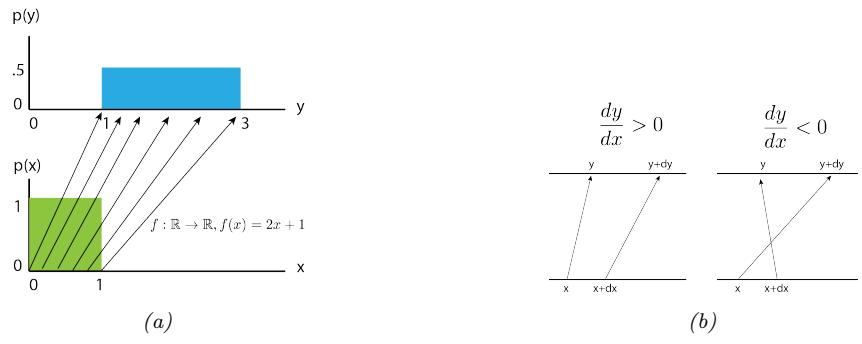
Figure 2.19: (a) Mapping a uniform pdf through the function f(x)=2x + 1. (b) Illustration of how two nearby points, x and x + dx, get mapped under f. If dy dx ^&gt; ⁰, the function is locally increasing, but if dy dx < 0, the function is locally decreasing. (In the latter case, if f(x) = y + dy, then f(x + dx) = y, since increasing x by dx should decrease the output by dy.) x + dx > x. From [Jan18]. Used with kind permission of Eric Jang.

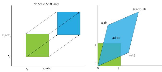
Figure 2.20: Illustration of an a”ne transformation applied to a unit square, f(x) = Ax+ b. (a) Here A = I. (b) Here b = 0. From [Jan18]. Used with kind permission of Eric Jang.

2.8.3.2 Change of variables: multivariate case

We can extend the previous results to multivariate distributions as follows. Let f be an invertible function that maps Rⁿ to Rⁿ, with inverse g. Suppose we want to compute the pdf of y = f(x). By analogy with the scalar case, we have

\[p\_y(\mathbf{y}) = p\_x(\mathbf{g}(\mathbf{y})) \left| \det \left[ \mathbf{J}\_g(\mathbf{y}) \right] \right| \tag{2.156}\]

where J^g = ^dg(y) ^dy^T is the Jacobian of g, and | det J(y)| is the absolute value of the determinant of J evaluated at y. (See Section 7.8.5 for a discussion of Jacobians.) In Exercise 3.6 you will use this formula to derive the normalization constant for a multivariate Gaussian.

Figure 2.20 illustrates this result in 2d, for the case where f(x) = Ax + b, where A = ’ a c b d( . We see that the area of the unit square changes by a factor of det(A) = ad ↑ bc, which is the area of the parallelogram.

As another example, consider transforming a density from Cartesian coordinates x = (x1, x2) to

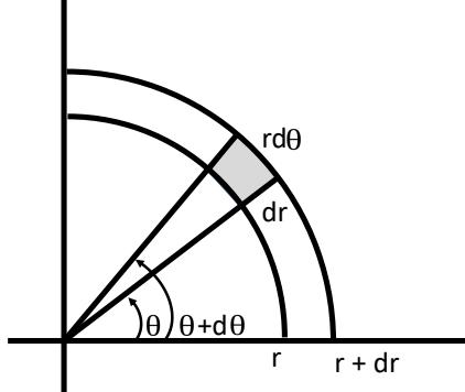
Figure 2.21: Change of variables from polar to Cartesian. The area of the shaded patch is r dr dε. Adapted from Figure 3.16 of [Ric95].

polar coordinates y = f(x1, x2), so g(r, ϖ)=(r cos ϖ, r sin ϖ). Then

\[\mathbf{J}\_g = \begin{pmatrix} \frac{\partial x\_1}{\partial r} & \frac{\partial x\_1}{\partial \theta} \\ \frac{\partial x\_2}{\partial r} & \frac{\partial x\_2}{\partial \theta} \end{pmatrix} = \begin{pmatrix} \cos \theta & -r \sin \theta \\ \sin \theta & r \cos \theta \end{pmatrix} \tag{2.157}\]

\[|\det(\mathbf{J}\_g)| = |r\cos^2\theta + r\sin^2\theta| = |r|\tag{2.158}\]

Hence

\[p\_{r, \theta}(r, \theta) = p\_{x\_1, x\_2}(r \cos \theta, r \sin \theta) \; r \tag{2.159}\]

To see this geometrically, notice that the area of the shaded patch in Figure 2.21 is given by

\[\Pr(r \le R \le r + dr, \theta \le \Theta \le \theta + d\theta) = p\_{r, \theta}(r, \theta) dr d\theta \tag{2.160}\]

In the limit, this is equal to the density at the center of the patch times the size of the patch, which is given by r dr dϖ. Hence

\[p\_{r, \theta}(r, \theta) \, dr \, d\theta = p\_{x\_1, x\_2}(r \cos \theta, r \sin \theta) \, r \, dr \, d\theta \tag{2.161}\]

2.8.4 Moments of a linear transformation

Suppose f is an a”ne function, so y = Ax + b. In this case, we can easily derive the mean and covariance of y as follows. First, for the mean, we have

\[\mathbb{E}\left[y\right] = \mathbb{E}\left[\mathbf{A}x + b\right] = \mathbf{A}\mu + \mathbf{b} \tag{2.162}\]

where µ = E [x]. If f is a scalar-valued function, f(x) = a^Tx + b, the corresponding result is

\[\mathbb{E}\left[\mathbf{a}^{\mathsf{T}}\mathbf{x} + b\right] = \mathbf{a}^{\mathsf{T}}\boldsymbol{\mu} + b\]

-	-	1	2	3	4	-	-
7	6	5	-	-	-	-	-	z0 = x0y0 = 5
-	7	6	5	-	-	-	-	z1 = x0y1 + x1y0 = 16
-	-	7	6	5	-	-	-	z2 = x0y2 + x1y1 + x2y0 = 34
-	-	-	7	6	5	-	-	z3 = x1y2 + x2y1 + x3y0 = 52
-	-	-	-	7	6	5	-	z4 = x2y2 + x3y1 = 45
-	-	-	-	-	7	6	5	z5 = x3y2 = 28

Table 2.4: Discrete convolution of x = [1, 2, 3, 4] with y = [5, 6, 7] to yield z = [5, 16, 34, 52, 45, 28]. In general, zⁿ = !^{↑ k}=→↑ ^xkyⁿ→^k. We see that this operation consists of “flipping” ^y and then “dragging” it over ^x, multiplying elementwise, and adding up the results.

For the covariance, we have

\[\text{Cov}\left[y\right] = \text{Cov}\left[\mathbf{A}x + \mathbf{b}\right] = \mathbf{A}\boldsymbol{\Sigma}\mathbf{A}^{\top} \tag{2.164}\]

where ! = Cov [x]. We leave the proof of this as an exercise.

As a special case, if y = a^Tx + b, we get

\[\mathbb{V}\left[y\right] = \mathbb{V}\left[\mathbf{a}^{\mathsf{T}}\mathbf{x} + b\right] = \mathbf{a}^{\mathsf{T}}\boldsymbol{\Sigma}\mathbf{a} \tag{2.165}\]

For example, to compute the variance of the sum of two scalar random variables, we can set a = [1, 1] to get

\[\mathbb{V}\left[x\_1 + x\_2\right] = \begin{pmatrix} 1 & 1 \end{pmatrix} \begin{pmatrix} \Sigma\_{11} & \Sigma\_{12} \\ \Sigma\_{21} & \Sigma\_{22} \end{pmatrix} \begin{pmatrix} 1 \\ 1 \end{pmatrix} \tag{2.166}\]

\[ \Sigma\_1 = \Sigma\_{11} + \Sigma\_{22} + 2\Sigma\_{12} = \mathbb{V}\left[x\_1\right] + \mathbb{V}\left[x\_2\right] + 2\text{Cov}\left[x\_1, x\_2\right] \tag{2.167} \]

Note, however, that although some distributions (such as the Gaussian) are completely characterized by their mean and covariance, in general we must use the techniques described above to derive the full distribution of y.

2.8.5 The convolution theorem

Let y = x¹ + x2, where x¹ and x² are independent rv’s. If these are discrete random variables, we can compute the pmf for the sum as follows:

\[p(y=j) = \sum\_{k} p(x\_1 = k)p(x\_2 = j - k) \tag{2.168}\]

for j = …, ↑2, ↑1, 0, 1, 2,….

If x¹ and x² have pdf’s p1(x1) and p2(x2), what is the distribution of y? The cdf for y is given by

\[P\_y(y^\*) = \Pr(y \le y^\*) = \int\_{-\infty}^{\infty} p\_1(x\_1) \left[ \int\_{-\infty}^{y^\*-x\_1} p\_2(x\_2) dx\_2 \right] dx\_1 \tag{2.169}\]

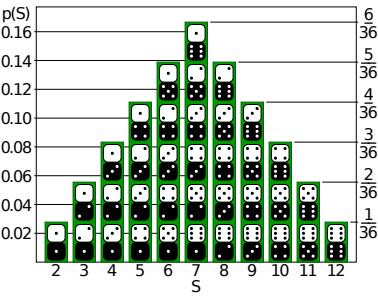
Figure 2.22: Distribution of the sum of two dice rolls, i.e., p(y) where y = x1+x² and xⁱ ↘ Unif({1, 2,…, 6}). From https: // en. wikipedia. org/ wiki/ Probability\_ distribution . Used with kind permission of Wikipedia author Tim Stellmach.

where we integrate over the region R defined by x¹ + x² < y↓. Thus the pdf for y is

\[p(y) = \left[\frac{d}{dy^\*} P\_y(y^\*)\right]\_{y^\* = y} = \int p\_1(x\_1) p\_2(y - x\_1) dx\_1 \tag{2.170}\]

where we used the rule of di”erentiating under the integral sign:

\[\frac{d}{dx}\int\_{a(x)}^{b(x)}f(t)dt = f(b(x))\frac{db(x)}{dx} - f(a(x))\frac{da(x)}{dx} \tag{2.171}\]

We can write Equation (2.170) as follows:

\[p = p\_1 \circledast p\_2 \tag{2.172}\]

where ↫ represents the convolution operator. For finite length vectors, the integrals become sums, and convolution can be thought of as a “flip and drag” operation, as illustrated in Table 2.4. Consequently, Equation (2.170) is called the convolution theorem.

For example, suppose we roll two dice, so p¹ and p² are both the discrete uniform distributions over {1, 2,…, 6}. Let y = x¹ + x² be the sum of the dice. We have

\[p(y=2) = p(x\_1=1)p(x\_2=1) = \frac{1}{6} \frac{1}{6} = \frac{1}{36} \tag{2.173}\]

\[p(y=3) = p(x\_1=1)p(x\_2=2) + p(x\_1=2)p(x\_2=1) = \frac{1}{6}\frac{1}{6} + \frac{1}{6}\frac{1}{6} = \frac{2}{36} \tag{2.174}\]

\[\cdots \tag{2.175}\]

Continuing in this way, we find p(y = 4) = 3/36, p(y = 5) = 4/36, p(y = 6) = 5/36, p(y = 7) = 6/36, p(y = 8) = 5/36, p(y = 9) = 4/36, p(y = 10) = 3/36, p(y = 11) = 2/36 and p(y = 12) = 1/36. See Figure 2.22 for a plot. We see that the distribution looks like a Gaussian; we explain the reasons for this in Section 2.8.6.

We can also compute the pdf of the sum of two continuous rv’s. For example, in the case of Gaussians, where ^{x1 ⇒ N} (µ1, ^{ε2 1}) and ^{x2 ⇒ N} (µ2, ^{ε2 2}), one can show (Exercise 2.4) that if y = x1+x²

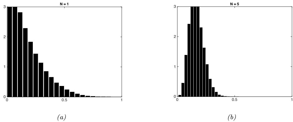
Figure 2.23: The central limit theorem in pictures. We plot a histogram of µˆ^{s N} = ¹ N !^{N n}=1 xns, where xns ↘ Beta(1, 5), for s = 1 : 10000. As N ≃ ⇐, the distribution tends towards a Gaussian. (a) N = 1. (b) N = 5. Adapted from Figure 2.6 of [Bis06]. Generated by centralLimitDemo.ipynb.

then

\[p(y) = \mathcal{N}(x\_1|\mu\_1, \sigma\_1^2) \otimes \mathcal{N}(x\_2|\mu\_2, \sigma\_2^2) = \mathcal{N}(y|\mu\_1 + \mu\_2, \sigma\_1^2 + \sigma\_2^2) \tag{2.176}\]

Hence the convolution of two Gaussians is a Gaussian.

2.8.6 Central limit theorem

Now consider N random variables with pdf’s (not necessarily Gaussian) pn(x), each with mean µ and variance ε². We assume each variable is independent and identically distributed or iid for short, which means ^{Xn ⇒ p}(X) are independent samples from the same distribution. Let ^{SN =} $^{N n}=1 Xⁿ be the sum of the rv’s. One can show that, as N increases, the distribution of this sum approaches

\[p(S\_N = u) = \frac{1}{\sqrt{2\pi N \sigma^2}} \exp\left(-\frac{(u - N\mu)^2}{2N\sigma^2}\right) \tag{2.177}\]

Hence the distribution of the quantity

\[Z\_N \triangleq \frac{S\_N - N\mu}{\sigma \sqrt{N}} = \frac{\overline{X} - \mu}{\sigma / \sqrt{N}}\tag{2.178}\]

converges to the standard normal, where X = S^N /N is the sample mean. This is called the central limit theorem. See e.g., [Jay03, p222] or [Ric95, p169] for a proof.

In Figure 2.23 we give an example in which we compute the sample mean of rv’s drawn from a beta distribution. We see that the sampling distribution of this mean rapidly converges to a Gaussian distribution.

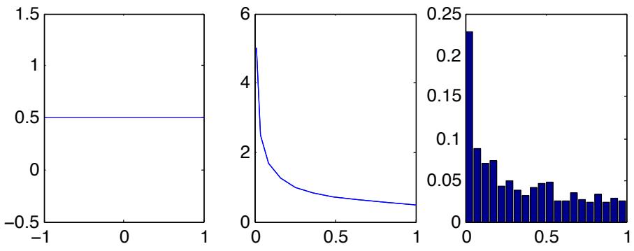
Figure 2.24: Computing the distribution of y = x², where p(x) is uniform (left). The analytic result is shown in the middle, and the Monte Carlo approximation is shown on the right. Generated by change\_of\_vars\_demo1d.ipynb.

2.8.7 Monte Carlo approximation

Suppose x is a random variable, and y = f(x) is some function of x. It is often di”cult to compute the induced distribution p(y) analytically. One simple but powerful alternative is to draw a large number of samples from the x’s distribution, and then to use these samples (instead of the distribution) to approximate p(y).

For example, suppose ^{x ⇒} Unif(↑1, 1) and ^y = ^f(x) = ^x2. We can approximate ^p(y) by drawing many samples from p(x) (using a uniform random number generator), squaring them, and computing the resulting empirical distribution, which is given by

\[p\_S(y) \triangleq \frac{1}{N\_s} \sum\_{s=1}^{N\_s} \delta(y - y\_s) \tag{2.179}\]

This is just an equally weighted “sum of spikes”, each centered on one of the samples (see Section 2.7.6). By using enough samples, we can approximate p(y) rather well. See Figure 2.24 for an illustration.

This approach is called a Monte Carlo approximation to the distribution. (The term “Monte Carlo” comes from the name of a famous gambling casino in Monaco.) Monte Carlo techniques were first developed in the area of statistical physics — in particular, during development of the atomic bomb — but are now widely used in statistics and machine learning as well. More details can be found in the sequel to this book, [Mur23], as well as specialized books on the topic, such as [Liu01; RC04; KTB11; BZ20].

2.9 Exercises

Exercise 2.1 [Conditional independence † ] (Source: Koller.)

1. Let H ⇒ {1,…,K} be a discrete random variable, and let e¹ and e² be the observed values of two other

random variables E¹ and E2. Suppose we wish to calculate the vector

\[\vec{P}(H|e\_1, e\_2) = (P(H = 1|e\_1, e\_2), \dots, P(H = K|e\_1, e\_2))\]

Which of the following sets of numbers are su!cient for the calculation?

• 1. P(e1, e2), P(H), P(e1|H), P(e2|H)
• 2. P(e1, e2), P(H), P(e1, e2|H)
• 3. P(e1|H), P(e2|H), P(H)
• 2. Now suppose we now assume E¹ ↓ E2|H (i.e., E¹ and E² are conditionally independent given H). Which of the above 3 sets are su!cient now?

Show your calculations as well as giving the final result. Hint: use Bayes rule.

Exercise 2.2 [Pairwise independence does not imply mutual independence]

We say that two random variables are pairwise independent if

\[p(X\_2|X\_1) = p(X\_2) \tag{2.180}\]

and hence

\[p(X\_2, X\_1) = p(X\_1)p(X\_2|X\_1) = p(X\_1)p(X\_2) \tag{2.181}\]

We say that n random variables are mutually independent if

\[p(X\_i|X\_S) = p(X\_i) \quad \forall S \subseteq \{1, \ldots, n\} \; \vert \; \{i\} \tag{2.182}\]

and hence

\[p(X\_{1:n}) = \prod\_{i=1}^{n} p(X\_i) \tag{2.183}\]

Show that pairwise independence between all pairs of variables does not necessarily imply mutual independence. It su!ces to give a counter example.

Exercise 2.3 [Conditional independence i” joint factorizes † ]

In the text we said X ↓ Y |Z i”

\[p(x,y|z) = p(x|z)p(y|z) \tag{2.184}\]

for all x, y, z such that p(z) > 0. Now prove the following alternative definition: X ↓ Y |Z i” there exist functions g and h such that

\[p(x,y|z) = g(x,z)h(y,z)\tag{2.185}\]

for all x, y, z such that p(z) > 0.

Exercise 2.4 [Convolution of two Gaussians is a Gaussian]

Show that the convolution of two Gaussians is a Gaussian, i.e.,

\[p(y) = \mathcal{N}(x\_1|\mu\_1, \sigma\_1^2) \otimes \mathcal{N}(x\_2|\mu\_2, \sigma\_2^2) = \mathcal{N}(y|\mu\_1 + \mu\_2, \sigma\_1^2 + \sigma\_2^2) \tag{2.186}\]

where ^{y = x1 + x}2, ^x1 ↘ ^N (µ1, ^{ϑ2 1}) and ^x2 ↘ ^N (µ2, ^{ϑ2 2}) are independent rv’s.

Exercise 2.5 [Expected value of the minimum of two rv’s † ]

Suppose X, Y are two points sampled independently and uniformly at random from the interval [0, 1]. What is the expected location of the leftmost point?

Exercise 2.6 [Variance of a sum]

Show that the variance of a sum is

\[\mathbb{V}\left[X+Y\right] = \mathbb{V}\left[X\right] + \mathbb{V}\left[Y\right] + 2\text{Cov}\left[X,Y\right],\tag{2.187}\]

where Cov [X, Y ] is the covariance between X and Y .

Exercise 2.7 [Deriving the inverse gamma density † ]

Let X ↘ Ga(a, b), and Y = 1/X. Derive the distribution of Y .

Exercise 2.8 [Mean, mode, variance for the beta distribution]

Suppose ε ↘ Beta(a, b). Show that the mean, mode and variance are given by

\[\mathbb{E}\left[\theta\right] = \frac{a}{a+b} \tag{2.188}\]

\[\mathbb{V}\left[\theta\right] = \frac{ab}{(a+b)^2(a+b+1)}\tag{2.189}\]

\[\text{dmode}\left[\theta\right] = \frac{a-1}{a+b-2} \tag{2.190}\]

Exercise 2.9 [Bayes rule for medical diagnosis † ]

After your yearly checkup, the doctor has bad news and good news. The bad news is that you tested positive for a serious disease, and that the test is 99% accurate (i.e., the probability of testing positive given that you have the disease is 0.99, as is the probability of testing negative given that you don’t have the disease). The good news is that this is a rare disease, striking only one in 10,000 people. What are the chances that you actually have the disease? (Show your calculations as well as giving the final result.)

Exercise 2.10 [Legal reasoning]

(Source: Peter Lee.) Suppose a crime has been committed. Blood is found at the scene for which there is no innocent explanation. It is of a type which is present in 1% of the population.

• 1. The prosecutor claims: “There is a 1% chance that the defendant would have the crime blood type if he were innocent. Thus there is a 99% chance that he is guilty”. This is known as the prosecutor’s fallacy. What is wrong with this argument?
• 2. The defender claims: “The crime occurred in a city of 800,000 people. The blood type would be found in approximately 8000 people. The evidence has provided a probability of just 1 in 8000 that the defendant is guilty, and thus has no relevance.” This is known as the defender’s fallacy. What is wrong with this argument?

Exercise 2.11 [Probabilities are sensitive to the form of the question that was used to generate the answer † ]

(Source: Minka.) My neighbor has two children. Assuming that the gender of a child is like a coin flip, it is most likely, a priori, that my neighbor has one boy and one girl, with probability 1/2. The other possibilities—two boys or two girls—have probabilities 1/4 and 1/4.

• 1. Suppose I ask him whether he has any boys, and he says yes. What is the probability that one child is a girl?
• b. Suppose instead that I happen to see one of his children run by, and it is a boy. What is the probability that the other child is a girl?

Exercise 2.12 [Normalization constant for a 1D Gaussian]

The normalization constant for a zero-mean Gaussian is given by

\[Z = \int\_{a}^{b} \exp\left(-\frac{x^2}{2\sigma^2}\right) dx\tag{2.191}\]

where a = ↑⇐ and b = ⇐. To compute this, consider its square

\[Z^2 = \int\_a^b \int\_a^b \exp\left(-\frac{x^2 + y^2}{2\sigma^2}\right) dx dy\tag{2.192}\]

Let us change variables from cartesian (x, y) to polar (r, ε) using x = r cos ε and y = r sin ε. Since dxdy = rdrdε, and cos²ε + sin² ε = 1, we have

\[Z^2 = \int\_0^{2\pi} \int\_0^{\infty} r \exp\left(-\frac{r^2}{2\sigma^2}\right) dr d\theta \tag{2.193}\]

Evaluate this integral and hence show ^{Z = ↔︎} ϑ²2ς. Hint 1: separate the integral into a product of two terms, the first of which (involving dε) is constant, so is easy. Hint 2: if u = e→r2/2ε² then du/dr ^{= ↑ 1 ε2} re→r2/2ε² , so the second integral is also easy (since & u^↓ (r)dr = u(r)).

3 Probability: Multivariate Models

3.1 Joint distributions for multiple random variables

In this section, we discuss various ways to measure the dependence of one or more variables on each other.

3.1.1 Covariance

The covariance between two rv’s X and Y measures the degree to which X and Y are (linearly) related. Covariance is defined as

\[\operatorname{Cov}\left[X,Y\right] \stackrel{\Delta}{=} \operatorname{E}\left[ (X-\mathbb{E}\left[X\right])(Y-\mathbb{E}\left[Y\right]) \right] = \operatorname{E}\left[XY\right] - \operatorname{E}\left[X\right]\operatorname{E}\left[Y\right] \tag{3.1}\]

If x is a D-dimensional random vector, its covariance matrix is defined to be the following symmetric, positive semi definite matrix:

\[\mathbb{E}\left[\text{Cov}\left[\mathbf{z}\right]\triangleq\mathbb{E}\left[(\mathbf{z}-\mathbb{E}\left[\mathbf{z}\right])(\mathbf{z}-\mathbb{E}\left[\mathbf{z}\right])^{\mathsf{T}}\right]\triangleq\mathbf{\Sigma}\right] \tag{3.2}\]

\[\begin{aligned} &= \begin{pmatrix} \mathbb{V}\left[X\_1\right] & \text{Cov}\left[X\_1, X\_2\right] & \cdots & \text{Cov}\left[X\_1, X\_D\right] \\ \text{Cov}\left[X\_2, X\_1\right] & \mathbb{V}\left[X\_2\right] & \cdots & \text{Cov}\left[X\_2, X\_D\right] \\ \vdots & \vdots & \ddots & \vdots \\ \text{Cov}\left[X\_D, X\_1\right] & \text{Cov}\left[X\_D, X\_2\right] & \cdots & \mathbb{V}\left[X\_D\right] \end{pmatrix} \end{aligned} \tag{3.3}\]

from which we get the important result

\[\mathbb{E}\left[x\boldsymbol{x}^{\mathsf{T}}\right] = \boldsymbol{\Sigma} + \mu\boldsymbol{\mu}^{\mathsf{T}} \tag{3.4}\]

Another useful result is that the covariance of a linear transformation is given by

\[\text{Cov}\left[\mathbf{A}\mathbf{x} + \mathbf{b}\right] = \mathbf{A}\text{Cov}\left[\mathbf{x}\right]\mathbf{A}^{\top}\tag{3.5}\]

as shown in Exercise 3.4.

The cross-covariance between two random vectors is defined as

\[\mathbb{E}\left[\text{Cov}\left[\mathbf{z},\mathbf{y}\right]\right] = \mathbb{E}\left[(\mathbf{z} - \mathbb{E}\left[\mathbf{z}\right])(\mathbf{y} - \mathbb{E}\left[\mathbf{y}\right])^{\mathsf{T}}\right] \tag{3.6}\]

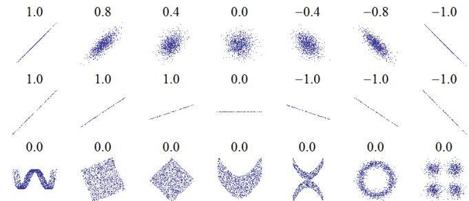
Figure 3.1: Several sets of (x, y) points, with the correlation coe”cient of x and y for each set. Note that the correlation reflects the noisiness and direction of a linear relationship (top row), but not the slope of that relationship (middle), nor many aspects of nonlinear relationships (bottom). (Note: the figure in the center has a slope of 0 but in that case the correlation coe”cient is undefined because the variance of Y is zero.) From https: // en. wikipedia. org/ wiki/ Pearson\_ correlation\_ coefficient . Used with kind permission of Wikipedia author Imagecreator.

3.1.2 Correlation

Covariances can be between negative and positive infinity. Sometimes it is more convenient to work with a normalized measure, with a finite lower and upper bound. The (Pearson) correlation coe!cient between X and Y is defined as

\[\rho \triangleq \text{corr}\left[X, Y\right] \triangleq \frac{\text{Cov}\left[X, Y\right]}{\sqrt{\mathbb{V}\left[X\right]\mathbb{V}\left[Y\right]}}\tag{3.7}\]

One can show (Exercise 3.2) that ↑1 ↘ ς ↘ 1.

One can also show that corr [X, Y ] = 1 if and only if Y = aX + b (and a > 0) for some parameters a and b, i.e., if there is a linear relationship between X and Y (see Exercise 3.3). Intuitively one might expect the correlation coe”cient to be related to the slope of the regression line, i.e., the coe”cient a in the expression Y = aX + b. However, as we show in Equation (11.27), the regression coe”cient is in fact given by a = Cov [X, Y ] /V [X]. In Figure 3.1, we show that the correlation coe”cient can be 0 for strong, but nonlinear, relationships. (Compare to Figure 6.6.) Thus a better way to think of the correlation coe”cient is as a degree of linearity. (See correlation2d.ipynb for a demo to illustrate this idea.)

In the case of a vector x of related random variables, the correlation matrix is given by

\[\operatorname{corr}(\mathbf{z}) = \begin{pmatrix} 1 & \frac{\mathbb{E}[(X\_1 - \mu\_1)(X\_2 - \mu\_2)]}{\sigma\_1 \sigma\_2} & \cdots & \frac{\mathbb{E}[(X\_1 - \mu\_1)(X\_D - \mu\_D)]}{\sigma\_1 \sigma\_D} \\ \frac{\mathbb{E}[(X\_2 - \mu\_2)(X\_1 - \mu\_1)]}{\sigma\_2 \sigma\_1} & 1 & \cdots & \frac{\mathbb{E}[(X\_2 - \mu\_2)(X\_D - \mu\_D)]}{\sigma\_2 \sigma\_D} \\ \vdots & \vdots & \ddots & \vdots \\ \frac{\mathbb{E}[(X\_D - \mu\_D)(X\_1 - \mu\_1)]}{\sigma\_D \sigma\_1} & \frac{\mathbb{E}[(X\_D - \mu\_D)(X\_2 - \mu\_2)]}{\sigma\_D \sigma\_2} & \cdots & 1 \end{pmatrix} \tag{3.8}\]

This can be written more compactly as

\[\text{corr}(\mathbf{z}) = (\text{diag}(\mathbf{K}\_{xx}))^{-\frac{1}{2}} \mathbf{K}\_{xx} (\text{diag}(\mathbf{K}\_{xx}))^{-\frac{1}{2}} \tag{3.9}\]

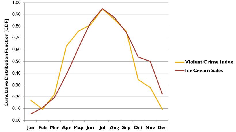
Figure 3.2: Examples of spurious correlation between causally unrelated time series. Consumption of ice cream (red) and violent crime rate (yellow). over time. From http: // icbseverywhere. com/ blog/ 2014/ 10/ the-logic-of-causal-conclusions/ . Used with kind permission of Barbara Drescher.

where Kxx is the auto-covariance matrix

\[\mathbf{K}\_{xx} = \boldsymbol{\Sigma} = \mathbb{E}\left[ (\mathbf{z} - \mathbb{E}\left[\boldsymbol{x}\right])(\mathbf{z} - \mathbb{E}\left[\boldsymbol{x}\right])^{\mathsf{T}} \right] = \mathbf{R}\_{xx} - \mu \boldsymbol{\mu}^{\mathsf{T}} \tag{3.10}\]

and Rxx = E + xx^T, is the autocorrelation matrix.

3.1.3 Uncorrelated does not imply independent

If X and Y are independent, meaning p(X, Y ) = p(X)p(Y ), then Cov [X, Y ] = 0, and hence corr [X, Y ] = 0. So independent implies uncorrelated. However, the converse is not true: uncorrelated does not imply independent. For example, let ^{X ⇒ U}(↑1, 1) and ^{Y = X2}. Clearly ^Y is dependent on X (in fact, Y is uniquely determined by X), yet one can show (Exercise 3.1) that corr [X, Y ] = 0. Some striking examples of this fact are shown in Figure 3.1. This shows several data sets where there is clear dependence between X and Y , and yet the correlation coe”cient is 0. A more general measure of dependence between random variables is mutual information, discussed in Section 6.3. This is zero only if the variables truly are independent.

3.1.4 Correlation does not imply causation

It is well known that “correlation does not imply causation”. For example, consider Figure 3.2. In red, we plot x1:^T , where x^t is the amount of ice cream sold in month t. In yellow, we plot y1:^T , where y^t is the violent crime rate in month t. (Quantities have been rescaled to make the plots overlap.) We see a strong correlation between these signals. Indeed, it is sometimes claimed that “eating ice cream causes murder” [Pet13]. Of course, this is just a spurious correlation, due to a hidden common cause, namely the weather. Hot weather increases ice cream sales, for obvious

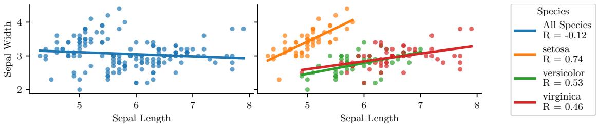
Figure 3.3: Illustration of Simpson’s paradox on the Iris dataset. (Left) Overall, y (sepal width) decreases with x (sepal length). (Right) Within each group, y increases with x. Generated by simpsons\_paradox.ipynb.

reasons. Hot weather also increases violent crime; the reason for this is hotly (ahem) debated; some claim it is due to an increase in anger [And01], but other claim it is merely due to more people being outside [Ash18], where most murders occur.

Another famous example concerns the positive correlation between birth rates and the presence of storks (a kind of bird). This has given rise to the urban legend that storks deliver babies [Mat00]. Of course, the true reason for the correlation is more likely due to hidden factors, such as increased living standards and hence more food. Many more amusing examples of such spurious correlations can be found in [Vig15].

These examples serve as a “warning sign”, that we should not treat the ability for x to predict y as an indicator that x causes y.

3.1.5 Simpson’s paradox

Simpson’s paradox says that a statistical trend or relationship that appears in several di!erent groups of data can disappear or reverse sign when these groups are combined. This results in counterintuitive behavior if we misinterpret claims of statistical dependence in a causal way.

A visualization of the paradox is given in Figure 3.3. Overall, we see that y decreases with x, but within each subpopulation, y increases with x.

For a recent real-world example of Simpson’s paradox in the context of COVID-19, consider Figure 3.4(a). This shows that the case fatality rate (CFR) of COVID-19 in Italy is less than in China in each age group, but is higher overall. The reason for this is that there are more older people in Italy, as shown in Figure 3.4(b). In other words, Figure 3.4(a) shows p(F = 1|A, C), where A is age, C is country, and F = 1 is the event that someone dies from COVID-19, and Figure 3.4(b) shows p(A|C), which is the probability someone is in age bucket A for country C. Combining these, we find p(F = 1|C = Italy) > p(F = 1|C = China). See [KGS20] for more details.

3.2 The multivariate Gaussian (normal) distribution

The most widely used joint probability distribution for continuous random variables is the multivariate Gaussian or multivariate normal (MVN). This is mostly because it is mathematically convenient, but also because the Gaussian assumption is fairly reasonable in many cases (see the discussion in Section 2.6.4).

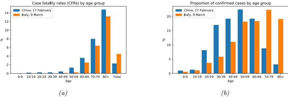
Figure 3.4: Illustration of Simpson’s paradox using COVID-19, (a) Case fatality rates (CFRs) in Italy and China by age group, and in aggregated form (“Total”, last pair of bars), up to the time of reporting (see legend). (b) Proportion of all confirmed cases included in (a) within each age group by country. From Figure 1 of [KGS20]. Used with kind permission of Julius von Kügelgen.

3.2.1 Definition

The MVN density is defined by the following:

\[\mathcal{N}(\boldsymbol{y}|\boldsymbol{\mu},\boldsymbol{\Sigma}) \stackrel{\scriptstyle \Delta}{=} \frac{1}{(2\pi)^{D/2}|\boldsymbol{\Sigma}|^{1/2}} \, \exp\left[ -\frac{1}{2} (\boldsymbol{y} - \boldsymbol{\mu})^{\mathsf{T}} \boldsymbol{\Sigma}^{-1} (\boldsymbol{y} - \boldsymbol{\mu}) \right] \tag{3.11}\]

where ^µ = ^E [y] ^{→ RD} is the mean vector, and ! = Cov [y] is the ^{D ↓ D} covariance matrix, defined as follows:

\[\mathbb{E}\left[\text{Cov}\left[\boldsymbol{y}\right]\triangleq\mathbb{E}\left[(\boldsymbol{y}-\mathbb{E}\left[\boldsymbol{y}\right])(\boldsymbol{y}-\mathbb{E}\left[\boldsymbol{y}\right])^{\mathsf{T}}\right]\right] \tag{3.12}\]

\[= \begin{pmatrix} \mathbb{V}\left[Y\_1\right] & \text{Cov}\left[Y\_1, Y\_2\right] & \cdots & \text{Cov}\left[Y\_1, Y\_D\right] \\ \text{Cov}\left[Y\_2, Y\_1\right] & \mathbb{V}\left[Y\_2\right] & \cdots & \text{Cov}\left[Y\_2, Y\_D\right] \\ \vdots & \vdots & \ddots & \vdots \\ \text{Cov}\left[Y\_D, Y\_1\right] & \text{Cov}\left[Y\_D, Y\_2\right] & \cdots & \mathbb{V}\left[Y\_D\right] \end{pmatrix} \tag{3.13}\]

where

\[\text{Cov}\left[Y\_i, Y\_j\right] \stackrel{\Delta}{=} \mathbb{E}\left[ (Y\_i - \mathbb{E}\left[Y\_i\right])(Y\_j - \mathbb{E}\left[Y\_j\right]) \right] = \mathbb{E}\left[Y\_i Y\_j\right] - \mathbb{E}\left[Y\_i\right]\mathbb{E}\left[Y\_j\right] \tag{3.14}\]

and V [Yi] = Cov [Yi, Yi]. From Equation (3.12), we get the important result

\[\mathbb{E}\left[\mathbf{y}\mathbf{y}^{\mathsf{T}}\right] = \Sigma + \mu\mu^{\mathsf{T}} \tag{3.15}\]

The normalization constant in Equation (3.11) ^Z = (2ϑ)D/²|!^{| 1}/² just ensures that the pdf integrates to 1 (see Exercise 3.6).

In 2d, the MVN is known as the bivariate Gaussian distribution. Its pdf can be represented as ^{y ⇒ N} (µ, !), where ^{y → R2}, ^{µ → R2} and

\[ \Sigma = \begin{pmatrix} \sigma\_1^2 & \rho \sigma\_1 \sigma\_2 \\ \rho \sigma\_1 \sigma\_2 & \sigma\_2^2 \end{pmatrix} \tag{3.16} \]

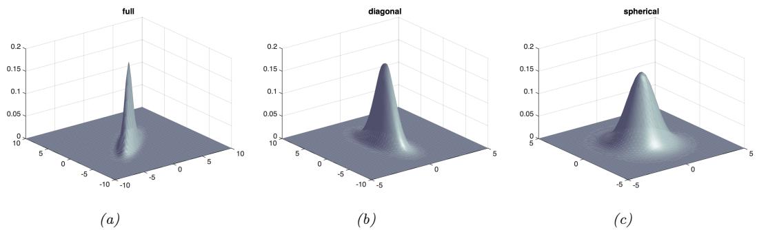
Figure 3.5: Visualization of a 2d Gaussian density as a surface plot. (a) Distribution using a full covariance matrix can be oriented at any angle. (b) Distribution using a diagonal covariance matrix must be parallel to the axis. (c) Distribution using a spherical covariance matrix must have a symmetric shape. Generated by gauss\_plot\_2d.ipynb.

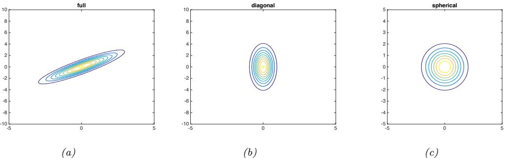
Figure 3.6: Visualization of a 2d Gaussian density in terms of level sets of constant probability density. (a) A full covariance matrix has elliptical contours. (b) A diagonal covariance matrix is an axis aligned ellipse. (c) A spherical covariance matrix has a circular shape. Generated by gauss\_plot\_2d.ipynb.

where ς is the correlation coe!cient, defined by

\[\text{corr}\left[Y\_1, Y\_2\right] \stackrel{\Delta}{=} \frac{\text{Cov}\left[Y\_1, Y\_2\right]}{\sqrt{\mathbb{V}\left[Y\_1\right]\mathbb{V}\left[Y\_2\right]}} = \frac{\sigma\_{12}^2}{\sigma\_1 \sigma\_2} \tag{3.17}\]

One can show (Exercise 3.2) that ↑1 ↘ corr [Y1, Y2] ↘ 1. Expanding out the pdf in the 2d case gives the following rather intimidating-looking result:

\[p(y\_1, y\_2) = \frac{1}{2\pi\sigma\_1\sigma\_2\sqrt{1-\rho^2}} \exp\left(-\frac{1}{2(1-\rho^2)} \times \\\\ \left[\frac{(y\_1-\mu\_1)^2}{\sigma\_1^2} + \frac{(y\_2-\mu\_2)^2}{\sigma\_2^2} - 2\rho\frac{(y\_1-\mu\_1)}{\sigma\_1}\frac{(y\_2-\mu\_2)}{\sigma\_2}\right]\right) \tag{3.18}\]

Figure 3.5 and Figure 3.6 plot some MVN densities in 2d for three di!erent kinds of covariance matrices. A full covariance matrix has D(D + 1)/2 parameters, where we divide by 2 since ! is

symmetric. (The reason for the elliptical shape is explained in Section 7.4.4, where we discuss the geometry of quadratic forms.) A diagonal covariance matrix has D parameters, and has 0s in the o!-diagonal terms. A spherical covariance matrix, also called isotropic covariance matrix, has the form ! = ε2ID, so it only has one free parameter, namely ε2.

3.2.2 Mahalanobis distance

In this section, we attempt to gain some insights into the geometric shape of the Gaussian pdf in multiple dimensions. To do this, we will consider the shape of the level sets of constant (log) probability.

The log probability at a specific point y is given by

\[\log p(y|\mu, \Sigma) = -\frac{1}{2}(y - \mu)^{\mathsf{T}}\Sigma^{-1}(y - \mu) + \text{const} \tag{3.19}\]

The dependence on y can be expressed in terms of the Mahalanobis distance % between y and µ, whose square is defined as follows:

\[ \Delta^2 \stackrel{\Delta}{=} (y - \mu)^\mathsf{T} \Sigma^{-1} (y - \mu) \tag{3.20} \]

Thus contours of constant (log) probability are equivalent to contours of constant Mahalanobis distance.

To gain insight into the contours of constant Mahalanobis distance, we exploit the fact that !, and hence ” = !^→1, are both positive definite matrices (by assumption). Consider the following eigendecomposition (Section 7.4) of !:

\[\Delta = \sum\_{d=1}^{D} \lambda\_d \mathbf{u}\_d \mathbf{u}\_d^T \tag{3.21}\]

We can similarly write

\[\boldsymbol{\Sigma}^{-1} = \sum\_{d=1}^{D} \frac{1}{\lambda\_d} \boldsymbol{u}\_d \boldsymbol{u}\_d^\top \tag{3.22}\]

Let us define z^d ↭ u^{T d}(y ↑ µ), so z = U(y ↑ µ). Then we can rewrite the Mahalanobis distance as follows:

\[\mathbb{E}\left(\boldsymbol{y}-\boldsymbol{\mu}\right)^{\mathsf{T}}\boldsymbol{\Sigma}^{-1}(\boldsymbol{y}-\boldsymbol{\mu})=(\boldsymbol{y}-\boldsymbol{\mu})^{\mathsf{T}}\left(\sum\_{d=1}^{D}\frac{1}{\lambda\_{d}}\boldsymbol{u}\_{d}\boldsymbol{u}\_{d}^{\mathsf{T}}\right)(\boldsymbol{y}-\boldsymbol{\mu})\tag{3.23}\]

\[=\sum\_{d=1}^{D} \frac{1}{\lambda\_d} (y-\mu)^{\mathsf{T}} u\_d u\_d^{\mathsf{T}} (y-\mu) = \sum\_{d=1}^{D} \frac{z\_d^2}{\lambda\_d} \tag{3.24}\]

As we discuss in Section 7.4.4, this means we can interpret the Mahalanobis distance as Euclidean distance in a new coordinate frame z in which we rotate y by U and scale by “.

For example, in 2d, let us consider the set of points (z1, z2) that satisfy this equation:

\[\frac{z\_1^2}{\lambda\_1} + \frac{z\_2^2}{\lambda\_2} = r\]

Since these points have the same Mahalanobis distance, they correspond to points of equal probability. Hence we see that the contours of equal probability density of a 2d Gaussian lie along ellipses. This is illustrated in Figure 7.6. The eigenvectors determine the orientation of the ellipse, and the eigenvalues determine how elongated it is.

3.2.3 Marginals and conditionals of an MVN *

Suppose y = (y1, y2) is jointly Gaussian with parameters

\[\boldsymbol{\mu} = \begin{pmatrix} \mu\_1 \\ \mu\_2 \end{pmatrix}, \quad \boldsymbol{\Sigma} = \begin{pmatrix} \Sigma\_{11} & \Sigma\_{12} \\ \Sigma\_{21} & \Sigma\_{22} \end{pmatrix}, \quad \boldsymbol{\Lambda} = \boldsymbol{\Sigma}^{-1} = \begin{pmatrix} \Lambda\_{11} & \Lambda\_{12} \\ \Lambda\_{21} & \Lambda\_{22} \end{pmatrix} \tag{3.26}\]

where ” is the precision matrix. Then the marginals are given by

\[\begin{aligned} p(y\_1) &= \mathcal{N}(y\_1|\mu\_1, \Sigma\_{11}) \\ p(y\_2) &= \mathcal{N}(y\_2|\mu\_2, \Sigma\_{22}) \end{aligned} \tag{3.27}\]

and the posterior conditional is given by

\[\begin{aligned} p(y\_1|y\_2) &= \mathcal{N}(y\_1|\mu\_{1|2}, \Sigma\_{1|2}) \\ \mu\_{1|2} &= \mu\_1 + \Sigma\_{12}\Sigma\_{21}^{-1}(y\_2 - \mu\_2) \\ &= \mu\_1 - \Lambda\_{11}^{-1}\Lambda\_{12}(y\_2 - \mu\_2) \\ &= \Sigma\_{1|2}\left(\Lambda\_{11}\mu\_1 - \Lambda\_{12}(y\_2 - \mu\_2)\right) \\ \Sigma\_{1|2} &= \Sigma\_{11} - \Sigma\_{12}\Sigma\_{22}^{-1}\Sigma\_{21} = \Lambda\_{11}^{-1} \end{aligned} \tag{3.28}\]

These equations are of such crucial importance in this book that we have put a box around them, so you can easily find them later. For the derivation of these results (which relies on computing the Schur complement !/!^{22 =} !^{11 ↑} !12!^{→1 22} !21), see Section 7.3.5.

We see that both the marginal and conditional distributions are themselves Gaussian. For the marginals, we just extract the rows and columns corresponding to y¹ or y2. For the conditional, we have to do a bit more work. However, it is not that complicated: the conditional mean is just a linear function of y2, and the conditional covariance is just a constant matrix that is independent of y2. We give three di!erent (but equivalent) expressions for the posterior mean, and two di!erent (but equivalent) expressions for the posterior covariance; each one is useful in di!erent circumstances.

3.2.4 Example: conditioning a 2d Gaussian

Let us consider a 2d example. The covariance matrix is

\[ \Sigma = \begin{pmatrix} \sigma\_1^2 & \rho \sigma\_1 \sigma\_2 \\ \rho \sigma\_1 \sigma\_2 & \sigma\_2^2 \end{pmatrix} \tag{3.29} \]

The marginal p(y1) is a 1D Gaussian, obtained by projecting the joint distribution onto the y¹ line:

\[p(y\_1) = \mathcal{N}(y\_1|\mu\_1, \sigma\_1^2) \tag{3.30}\]

Suppose we observe Y² = y2; the conditional p(y1|y2) is obtained by “slicing” the joint distribution through the Y² = y² line:

\[p(y\_1|y\_2) = N\left(y\_1|\mu\_1 + \frac{\rho\sigma\_1\sigma\_2}{\sigma\_2^2}(y\_2 - \mu\_2), \,\sigma\_1^2 - \frac{(\rho\sigma\_1\sigma\_2)^2}{\sigma\_2^2}\right) \tag{3.31}\]

If ε¹ = ε² = ε, we get

\[p(y\_1|y\_2) = \mathcal{N}\left(y\_1|\mu\_1 + \rho(y\_2 - \mu\_2), \ \sigma^2(1 - \rho^2)\right) \tag{3.32}\]

For example, suppose ς = 0.8, ε¹ = ε² = 1, µ¹ = µ² = 0, and y² = 1. We see that E [y1|y² = 1] = 0.8, which makes sense, since ς = 0.8 means that we believe that if y² increases by 1 (beyond its mean), then ^y1 increases by 0.8. We also see ^V [y1|y² = 1] = 1 ^{↑ 0}.8² = 0.36. This also makes sense: our uncertainty about y¹ has gone down, since we have learned something about y¹ (indirectly) by observing ^y2. If ^ς = 0, we get ^p(y1|y2) = ^N . ^y1|µ1, ^ε2 1 / , since y² conveys no information about y¹ if they are uncorrelated (and hence independent).

3.2.5 Example: Imputing missing values *

As an example application of the above results, suppose we observe some parts (dimensions) of y, with the remaining parts being missing or unobserved. We can exploit the correlation amongst the dimensions (encoded by the covariance matrix) to infer the missing entries; this is called missing value imputation.

Figure 3.7 shows a simple example. We sampled N = 10 vectors from a D = 8-dimensional Gaussian, and then deliberately “hid” 50% of the data. We then inferred the missing entries given the observed entries and the true model parameters.1 More precisely, for each example n in the data matrix, we compute p(yn,h|yn,v, ω), where v are the indices of the visible entries in that example, h are the remaining indices of the hidden entries, and ω = (µ, !). From this, we compute the marginal distribution of each missing variable i → h, p(yn,i|yn,v, ω). From the marginal, we compute the posterior mean, y¯n,i = E [yn,i|yn,v, ω].

The posterior mean represents our “best guess” about the true value of that entry, in the sense that it minimizes our expected squared error, as explained in Chapter 5. We can use V [yn,i|yn,v, ω] as a measure of confidence in this guess, although this is not shown. Alternatively, we could draw multiple posterior samples from p(yn,h|yn,v, ω); this is called multiple imputation, and provides a more robust estimate to downstream algorithms that consume the “filled in” data.

^1. In practice, we would need to estimate the parameters from the partially observed data. Unfortunately the MLE results in Section 4.2.6 no longer apply, but we can use the EM algorithm to derive an approximate MLE in the presence of missing data. See the sequel to this book for details.

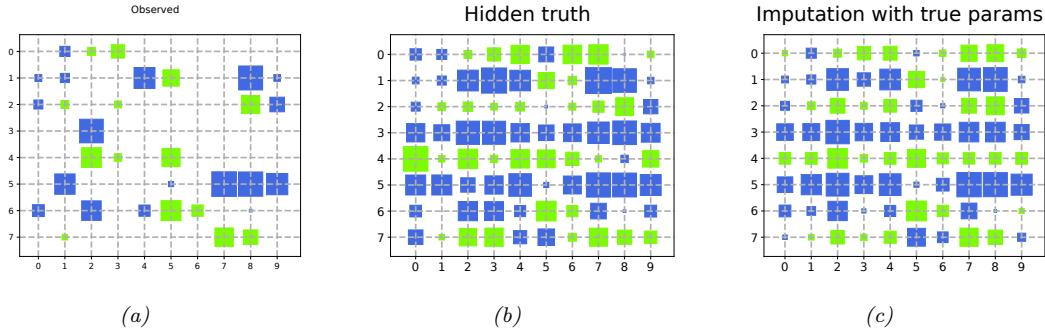
Figure 3.7: Illustration of data imputation using an MVN. Rows are features, columns are data samples (the transpose of the convention used in the text). (a) Visualization of the data matrix. Blank entries are missing (not observed). Blue are positive, green are negative. Area of the square is proportional to the value. (This is known as a Hinton diagram, named after Geo! Hinton, a famous ML researcher.) (b) True data matrix (hidden). (c) Mean of the posterior predictive distribution, based on partially observed data for that example (column), using the true model parameters. Generated by gauss\_imputation\_known\_params\_demo.ipynb.

3.3 Linear Gaussian systems *

In Section 3.2.3, we conditioned on noise-free observations to infer the posterior over the hidden parts of a Gaussian random vector. In this section, we extend this approach to handle noisy observations.

Let ^{z → RL} be an unknown vector of values, and ^{y → RD} be some noisy measurement of ^z. We assume these variables are related by the following joint distribution:

\[p(\mathbf{z}) = \mathcal{N}(\mathbf{z}|\boldsymbol{\mu}\_z, \boldsymbol{\Sigma}\_z) \tag{3.33}\]

\[p(y|z) = \mathcal{N}(y|\mathbf{W}z + \mathbf{b}, \Sigma\_y) \tag{3.34}\]

where W is a matrix of size D ↓ L. This is an example of a linear Gaussian system.

The corresponding joint distribution, p(z, y) = p(z)p(y|z), is a L + D dimensional Gaussian, with mean and covariance given by

\[\mu = \begin{pmatrix} \mu\_z \\ \mathbf{W}\mu\_z + \mathbf{b} \end{pmatrix} \tag{3.35}\]

\[ \Sigma = \begin{pmatrix} \Sigma\_z & \Sigma\_z \mathbf{W}^\top \\ \mathbf{W}\Sigma\_z & \Sigma\_y + \mathbf{W}\Sigma\_z \mathbf{W}^\top \end{pmatrix} \tag{3.36} \]

By applying the Gaussian conditioning formula in Equation (3.28) to the joint p(y, z) we can compute the posterior p(z|y), as we explain below. This can be interpreted as inverting the z ↔︎ y arrow in the generative model from latents to observations.

3.3.1 Bayes rule for Gaussians

The posterior over the latent is given by

\[\begin{aligned} p(\mathbf{z}|\mathbf{y}) &= \mathcal{N}(\mathbf{z}|\boldsymbol{\mu}\_{z|\mathbf{y}}, \boldsymbol{\Sigma}\_{z|\mathbf{y}})\\ \boldsymbol{\Sigma}\_{z|\mathbf{y}}^{-1} &= \boldsymbol{\Sigma}\_{z}^{-1} + \mathbf{W}^{\mathrm{T}} \boldsymbol{\Sigma}\_{y}^{-1} \mathbf{W} \\ \boldsymbol{\mu}\_{z|\mathbf{y}} &= \boldsymbol{\Sigma}\_{z|\mathbf{y}} [\mathbf{W}^{\mathrm{T}} \boldsymbol{\Sigma}\_{y}^{-1} \ (\mathbf{y} - \mathbf{b}) + \boldsymbol{\Sigma}\_{z}^{-1} \boldsymbol{\mu}\_{z}] \end{aligned} \tag{3.37}\]

This is known as Bayes rule for Gaussians. Furthermore, the normalization constant of the posterior is given by

\[p(\mathbf{y}) = \int \mathcal{N}(z|\boldsymbol{\mu}\_z, \boldsymbol{\Sigma}\_z) \mathcal{N}(y|\mathbf{W}z + \mathbf{b}, \boldsymbol{\Sigma}\_y) dz = \mathcal{N}(y|\mathbf{W}\boldsymbol{\mu}\_z + \mathbf{b}, \boldsymbol{\Sigma}\_y + \mathbf{W}\boldsymbol{\Sigma}\_z\mathbf{W}^\top) \tag{3.38}\]

We see that the Gaussian prior p(z), combined with the Gaussian likelihood p(y|z), results in a Gaussian posterior p(z|y). Thus Gaussians are closed under Bayesian conditioning. To describe this more generally, we say that the Gaussian prior is a conjugate prior for the Gaussian likelihood, since the posterior distribution has the same type as the prior. We discuss the notion of conjugate priors in more detail in Section 4.6.1.

In the sections below, we give various applications of this result. But first, we give the derivation.

3.3.2 Derivation *

We now derive Equation 3.37. The basic idea is to derive the joint distribution, p(z, y) = p(z)p(y|z), and then to use the results from Section 3.2.3 for computing p(z|y).

In more detail, we proceed as follows. The log of the joint distribution is as follows (dropping irrelevant constants):

\[\log p(\mathbf{z}, \mathbf{y}) = -\frac{1}{2} (\mathbf{z} - \boldsymbol{\mu}\_z)^T \boldsymbol{\Sigma}\_z^{-1} (\mathbf{z} - \boldsymbol{\mu}\_z) - \frac{1}{2} (\mathbf{y} - \mathbf{W}\mathbf{z} - \mathbf{b})^T \boldsymbol{\Sigma}\_y^{-1} (\mathbf{y} - \mathbf{W}\mathbf{z} - \mathbf{b}) \tag{3.39}\]

This is clearly a joint Gaussian distribution, since it is the exponential of a quadratic form.

Expanding out the quadratic terms involving z and y, and ignoring linear and constant terms, we have

\[Q = -\frac{1}{2}z^T \Sigma\_z^{-1} z - \frac{1}{2}y^T \Sigma\_y^{-1} y - \frac{1}{2}(\mathbf{W}z)^T \Sigma\_y^{-1} (\mathbf{W}z) + y^T \Sigma\_y^{-1} \mathbf{W}z \tag{3.40}\]

\[\mathbf{U} = -\frac{1}{2} \begin{pmatrix} \mathbf{z} \\ \mathbf{y} \end{pmatrix}^{T} \begin{pmatrix} \boldsymbol{\Sigma}\_{z}^{-1} + \mathbf{W}^{T} \boldsymbol{\Sigma}\_{y}^{-1} \mathbf{W} & -\mathbf{W}^{T} \boldsymbol{\Sigma}\_{y}^{-1} \\ -\boldsymbol{\Sigma}\_{y}^{-1} \mathbf{W} & \boldsymbol{\Sigma}\_{y}^{-1} \end{pmatrix} \begin{pmatrix} \mathbf{z} \\ \mathbf{y} \end{pmatrix} \tag{3.41}\]

\[\mathbf{y} = -\frac{1}{2} \begin{pmatrix} \mathbf{z} \\ \mathbf{y} \end{pmatrix}^T \boldsymbol{\Sigma}^{-1} \begin{pmatrix} \mathbf{z} \\ \mathbf{y} \end{pmatrix} \tag{3.42}\]

where the precision matrix of the joint is defined as

\[\boldsymbol{\Sigma}^{-1} = \begin{pmatrix} \boldsymbol{\Sigma}\_{z}^{-1} + \mathbf{W}^{T} \boldsymbol{\Sigma}\_{y}^{-1} \mathbf{W} & -\mathbf{W}^{T} \boldsymbol{\Sigma}\_{y}^{-1} \\ -\boldsymbol{\Sigma}\_{y}^{-1} \mathbf{W} & \boldsymbol{\Sigma}\_{y}^{-1} \end{pmatrix} \triangleq \boldsymbol{\Lambda} = \begin{pmatrix} \boldsymbol{\Lambda}\_{zz} & \boldsymbol{\Lambda}\_{zy} \\ \boldsymbol{\Lambda}\_{yz} & \boldsymbol{\Lambda}\_{yy} \end{pmatrix} \tag{3.43}\]

From Equation 3.28, and using the fact that µ^y = Wµ^z + b, we have

\[p(\mathbf{z}|\mathbf{y}) = \mathcal{N}(\boldsymbol{\mu}\_{z|y}, \boldsymbol{\Sigma}\_{z|y}) \tag{3.44}\]

\[ \Sigma\_{z|y} = \Lambda\_{zz}^{-1} = (\Sigma\_z^{-1} + \mathbf{W}^T \Sigma\_y^{-1} \mathbf{W})^{-1} \tag{3.45} \]

\[ \mu\_{z|y} = \Sigma\_{z|y} \left( \Lambda\_{zz} \mu\_z - \Lambda\_{zy} (y - \mu\_y) \right) \tag{3.46} \]

\[\mathbf{y} = \boldsymbol{\Sigma}\_{z|y} \left( \boldsymbol{\Sigma}\_{z}^{-1} \boldsymbol{\mu}\_{z} + \mathbf{W}^{\top} \boldsymbol{\Sigma}\_{y}^{-1} \mathbf{W} \boldsymbol{\mu}\_{z} + \mathbf{W}^{\top} \boldsymbol{\Sigma}\_{y}^{-1} (y - \boldsymbol{\mu}\_{y}) \right) \tag{3.47}\]

\[=\boldsymbol{\Sigma}\_{z|y}\left(\boldsymbol{\Sigma}\_{z}^{-1}\boldsymbol{\mu}\_{z}+\boldsymbol{\mathsf{W}}^{\mathsf{T}}\boldsymbol{\Sigma}\_{y}^{-1}(\boldsymbol{\mathsf{W}}\boldsymbol{\mu}\_{z}+\boldsymbol{y}-\boldsymbol{\mu}\_{y})\right)\tag{3.48}\]

\[\mathbf{y} = \boldsymbol{\Sigma}\_{z|y} \left( \boldsymbol{\Sigma}\_{z}^{-1} \boldsymbol{\mu}\_{z} + \mathbf{W}^{T} \boldsymbol{\Sigma}\_{y}^{-1} (\boldsymbol{y} - \mathbf{b}) \right) \tag{3.49}\]

3.3.2.1 Completing the square

When working with linear Gaussian systems, it is common to use an algebraic trick called completing the square. In the scalar case, this says that we can write a quadratic function of the form

\[f(x) = ax^2 + bx + c\]

as follows:

\[ax^2 + bx + c = a(x - h)^2 + k\]

\[\begin{aligned} h &= -\frac{b}{2a} \\ k &= c - \frac{b^2}{4a} \end{aligned}\]

In the vector case, this says we write a quadratic function of the form

\[f(x) = x^\top \mathbf{A} x + x^\top b + c\]

as follows:

\[\begin{aligned} x^\top \mathbf{A} x + x^\top b + c &= (x - h)^\top \mathbf{A} (x - h) + k \\\ h &= -\frac{1}{2} \mathbf{A}^{-1} b \\\ k &= c - \frac{1}{4} \mathbf{b}^\top \mathbf{A}^{-1} b \end{aligned}\]

This trick will be used in more advanced derivations.

3.3.3 Example: Inferring an unknown scalar

Suppose we make N noisy measurements yⁱ of some underlying quantity z; let us assume the measurement noise has fixed precision φ^y = 1/ε², so the likelihood is

\[p(y\_i|z) = \mathcal{N}(y\_i|z, \lambda\_y^{-1})\tag{3.50}\]

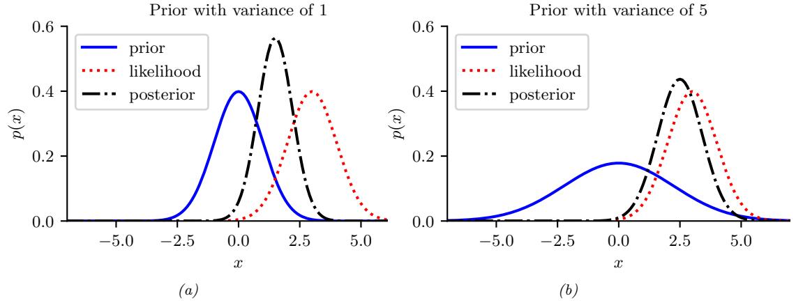
Figure 3.8: Inference about z given a noisy observation y = 3. (a) Strong prior N (0, 1). The posterior mean is “shrunk” towards the prior mean, which is 0. (b) Weak prior N (0, 5). The posterior mean is similar to the MLE. Generated by gauss\_infer\_1d.ipynb.

Now let us use a Gaussian prior for the value of the unknown source:

\[p(z) = \mathcal{N}(z|\mu\_0, \lambda\_0^{-1})\tag{3.51}\]

We want to compute ^p(z|y1,…,y^N , ^ε2). We can convert this to a form that lets us apply Bayes rule for Gaussians by defining y = (y1,…,y^N ), W = 1^N (an N ↓ 1 column vector of 1’s), and !^{→1 y} = diag(φyI). Then we get

\[p(z|\mathbf{y}) = \mathcal{N}(z|\mu\_N, \lambda\_N^{-1})\tag{3.52}\]

\[ \lambda\_N = \lambda\_0 + N\lambda\_y \tag{3.53} \]

\[ \mu\_N = \frac{N\lambda\_y \overline{y} + \lambda\_0 \mu\_0}{\lambda\_N} = \frac{N\lambda\_y}{N\lambda\_y + \lambda\_0} \overline{y} + \frac{\lambda\_0}{N\lambda\_y + \lambda\_0} \mu\_0 \tag{3.54} \]

These equations are quite intuitive: the posterior precision φ^N is the prior precision φ⁰ plus N units of measurement precision φy. Also, the posterior mean µ^N is a convex combination of the MLE y and the prior mean µ0. This makes it clear that the posterior mean is a compromise between the MLE and the prior. If the prior is weak relative to the signal strength (φ⁰ is small relative to φy), we put more weight on the MLE. If the prior is strong relative to the signal strength (φ⁰ is large relative to φy), we put more weight on the prior. This is illustrated in Figure 3.8.

Note that the posterior mean is written in terms of Nφyy, so having N measurements each of precision φ^y is like having one measurement with value y and precision Nφy.

We can rewrite the results in terms of the posterior variance, rather than posterior precision, as

follows:

\[p(z|\mathcal{D}, \sigma^2) = \mathcal{N}(z|\mu\_N, \tau\_N^2) \tag{3.55}\]

\[ \tau\_N^2 = \frac{1}{\frac{N}{\sigma^2} + \frac{1}{\tau\_0^2}} = \frac{\sigma^2 \tau\_0^2}{N\tau\_0^2 + \sigma^2} \tag{3.56} \]

\[ \mu\_N = \tau\_N^2 \left(\frac{\mu\_0}{\tau\_0^2} + \frac{N\overline{y}}{\sigma^2}\right) = \frac{\sigma^2}{N\tau\_0^2 + \sigma^2} \mu\_0 + \frac{N\tau\_0^2}{N\tau\_0^2 + \sigma^2} \overline{y} \tag{3.57} \]

where τ ^{2 0} = 1/φ⁰ is the prior variance and τ ^{2 N} = 1/φ^N is the posterior variance.

We can also compute the posterior sequentially, by updating after each observation. If N = 1, we can rewrite the posterior after seeing a single observation as follows (where we define $^y = ε², $⁰ = τ ^{2 0} and $¹ = τ ^{2 1} to be the variances of the likelihood, prior and posterior):

\[p(z|y) = \mathcal{N}(z|\mu\_1, \Sigma\_1) \tag{3.58}\]

\[ \Sigma\_1 = \left(\frac{1}{\Sigma\_0} + \frac{1}{\Sigma\_y}\right)^{-1} = \frac{\Sigma\_y \Sigma\_0}{\Sigma\_0 + \Sigma\_y} \tag{3.59} \]

\[ \mu\_1 = \Sigma\_1 \left(\frac{\mu\_0}{\Sigma\_0} + \frac{y}{\Sigma\_y}\right) \tag{3.60} \]

We can rewrite the posterior mean in 3 di!erent ways:

\[ \mu\_1 = \frac{\Sigma\_y}{\Sigma\_y + \Sigma\_0} \mu\_0 + \frac{\Sigma\_0}{\Sigma\_y + \Sigma\_0} y \tag{3.61} \]

\[\mu\_0 = \mu\_0 + (y - \mu\_0) \frac{\Sigma\_0}{\Sigma\_y + \Sigma\_0} \tag{3.62}\]

\[y = y - (y - \mu\_0) \frac{\Sigma\_y}{\Sigma\_y + \Sigma\_0} \tag{3.63}\]

The first equation is a convex combination of the prior and the data. The second equation is the prior mean adjusted towards the data. The third equation is the data adjusted towards the prior mean; this is called shrinkage. These are all equivalent ways of expressing the tradeo! between likelihood and prior. If $⁰ is small relative to $y, corresponding to a strong prior, the amount of shrinkage is large (see Figure 3.8(a)), whereas if $⁰ is large relative to $y, corresponding to a weak prior, the amount of shrinkage is small (see Figure 3.8(b)).

Another way to quantify the amount of shrinkage is in terms of the signal-to-noise ratio, which is defined as follows:

\[\text{SNR} \triangleq \frac{\mathbb{E}\left[Z^2\right]}{\mathbb{E}\left[\epsilon^2\right]} = \frac{\Sigma\_0 + \mu\_0^2}{\Sigma\_y} \tag{3.64}\]

where z ⇒ N (µ0, $0) is the true signal, y = z + ▷ is the observed signal, and ▷ ⇒ N (0, $y) is the noise term.

3.3.4 Example: inferring an unknown vector

Suppose we have an unknown quantity of interest, ^{z → RD}, which we endow with a Gaussian prior, p(z) = N (µz, !z). If we “know nothing” about z a priori, we can set !^z = ∈I, which means we are

completely uncertain about what the value of z should be. (In practice, we can use a large but finite value for the covariance.) By symmetry, it seems reasonable to set µ^z = 0.

Now suppose we make N noisy but independent measurements of z, yⁿ ⇒ N (z, !y), each of size D. One can show that the likelihood of N observations can be represented by a single Gaussian evaluated at their average, y, provided we scale down the covariance by 1/N to compensate for the increased measurement precision, i.e.,

\[p(\mathcal{D}|\mathbf{z}) = \prod\_{n=1}^{N} \mathcal{N}(y\_n|\mathbf{z}, \boldsymbol{\Sigma}\_y) \propto \mathcal{N}(\overline{\mathbf{y}}|\mathbf{z}, \frac{1}{N}\boldsymbol{\Sigma}\_y) \tag{3.65}\]

To see why this is true, consider the case of two measurements. The log likelihood can then be written using canonical parameters as follows:2

\[\begin{split} \log(p(y\_1|\mathbf{z})p(y\_2|\mathbf{z})) &= K\_1 - \frac{1}{2} \left( \mathbf{z}^\mathsf{T} \Sigma\_y^{-1} \mathbf{z} - 2\mathbf{z}^\mathsf{T} \Sigma\_y^{-1} y\_1 \right) - \frac{1}{2} \left( \mathbf{z}^\mathsf{T} \Sigma\_y^{-1} \mathbf{z} - 2\mathbf{z}^\mathsf{T} \Sigma\_y^{-1} y\_1 \right) \\ &= K\_1 - \frac{1}{2} \left( \mathbf{z}^\mathsf{T} 2\Sigma\_y^{-1} \mathbf{z} - 2\mathbf{z}^\mathsf{T} \Sigma\_y^{-1} \left( y\_1 + y\_2 \right) \right) \\ &= K\_1 - \frac{1}{2} \left( \mathbf{z}^\mathsf{T} 2\Sigma\_y^{-1} \mathbf{z} - 2\mathbf{z}^\mathsf{T} 2\Sigma\_y^{-1} \bar{y} \right) \\ &= K\_2 + \log \mathcal{N}(\mathbf{z}|\bar{y}, \frac{\Sigma\_y}{2}) = K\_2 + \log \mathcal{N}(\bar{y}|\mathbf{z}, \frac{\Sigma\_y}{2}) \end{split}\]

where K¹ and K² are constants independent of z.

Using this, and setting W = I, b = 0, we can then use Bayes rule for Gaussian to compute the posterior over z:

\[p(\mathbf{z}|\mathbf{y}\_1, \dots, \mathbf{y}\_N) = \mathcal{N}(\mathbf{z}|\,\hat{\boldsymbol{\mu}}, \hat{\boldsymbol{\Sigma}}) \tag{3.66}\]

\[ \hat{\boldsymbol{\Sigma}}^{-1} = \boldsymbol{\Sigma}\_z^{-1} + N\boldsymbol{\Sigma}\_y^{-1} \tag{3.67} \]

\[ \hat{\boldsymbol{\mu}} = \hat{\boldsymbol{\Sigma}} \left( \boldsymbol{\Sigma}\_y^{-1} (N \overline{\boldsymbol{y}}) + \boldsymbol{\Sigma}\_z^{-1} \boldsymbol{\mu}\_z \right) \tag{3.68} \]

where ↭µ and ↭ ! are the parameters of the posterior.

Figure 3.9 gives a 2d example. We can think of z as representing the true, but unknown, location of an object in 2d space, such as a missile or airplane, and the yⁿ as being noisy observations, such as radar “blips”. As we receive more blips, we are better able to localize the source. (In the sequel to this book, [Mur23], we discuss the Kalman filter algorithm, which extends this idea to a temporal sequence of observations.)

The posterior uncertainty about each component of z location vector depends on how reliable the sensor is in each of these dimensions. In the above example, the measurement noise in dimension 1 is higher than in dimension 2, so we have more posterior uncertainty about z¹ (horizontal axis) than about z² (vertical axis).

^2. This derivation is due to Joaquin Rapela. See https://github.com/probml/pml-book/issues/512.

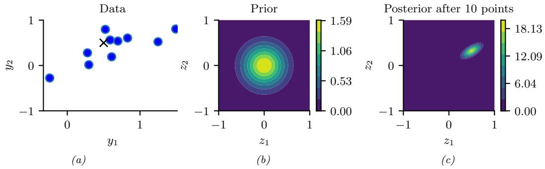
Figure 3.9: Illustration of Bayesian inference for a 2d Gaussian random vector z. (a) The data is generated from ^yn ↘ ^N (z, !y), where ^z = [0.5, ⁰.5]^T and !^y = 0.1[2, 1; 1, 1]). We assume the sensor noise covariance !^y is known but z is unknown. The black cross represents z. (b) The prior is p(z) = N (z|0, 0.1I2). (c) We show the posterior after 10 data points have been observed. Generated by gauss\_infer\_2d.ipynb.

3.3.5 Example: sensor fusion

In this section, we extend Section 3.3.4, to the case where we have multiple measurements, coming from di!erent sensors, each with di!erent reliabilities. That is, the model has the form

\[p(\mathbf{z}, \mathbf{y}) = p(\mathbf{z}) \prod\_{m=1}^{M} \prod\_{n=1}^{N\_m} \mathcal{N}(y\_{n,m}|\mathbf{z}, \boldsymbol{\Sigma}\_m) \tag{3.69}\]

where M is the number of sensors (measurement devices), and N^m is the number of observations from sensor ^m, and ^y = ^y1:N,1:^{M → RK}. Our goal is to combine the evidence together, to compute p(z|y). This is known as sensor fusion.

We now give a simple example, where there are just two sensors, so y¹ ⇒ N (z, !1) and y² ⇒ N (z, !2). Pictorially, we can represent this example as y¹ ▽ z ↔︎ y2. We can combine y¹ and y² into a single vector y, so the model can be represented as z ↔︎ [y1, y2], where p(y|z) = N (y|Wz, !y), where W = [I; I] and !^y = [!1, 0; 0, !2] are block-structured matrices. We can then apply Bayes’ rule for Gaussians to compute p(z|y).

Figure 3.10(a) gives a 2d example, where we set !¹ = !² = 0.01I2, so both sensors are equally reliable. In this case, the posterior mean is halfway between the two observations, y¹ and y2. In Figure 3.10(b), we set !¹ = 0.05I² and !² = 0.01I2, so sensor 2 is more reliable than sensor 1. In this case, the posterior mean is closer to y2. In Figure 3.10(c), we set

\[ \Sigma\_1 = 0.01 \begin{pmatrix} 10 & 1 \\ 1 & 1 \end{pmatrix}, \quad \Sigma\_2 = 0.01 \begin{pmatrix} 1 & 1 \\ 1 & 10 \end{pmatrix} \tag{3.70} \]

so sensor 1 is more reliable in the second component (vertical direction), and sensor 2 is more reliable in the first component (horizontal direction). In this case, the posterior mean uses y1’s vertical component and y2’s horizontal component.

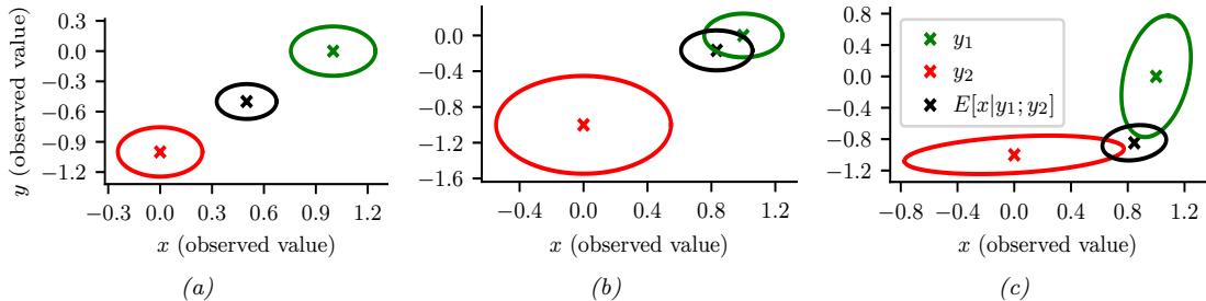
Figure 3.10: We observe y¹ = (0, ↑1) (red cross) and y² = (1, 0) (green cross) and estimate E [z|y1, y2] (black cross). (a) Equally reliable sensors, so the posterior mean estimate is in between the two circles. (b) Sensor 2 is more reliable, so the estimate shifts more towards the green circle. (c) Sensor 1 is more reliable in the vertical direction, Sensor 2 is more reliable in the horizontal direction. The estimate is an appropriate combination of the two measurements. Generated by sensor\_fusion\_2d.ipynb.

3.4 The exponential family *

In this section, we define the exponential family, which includes many common probability distributions. The exponential family plays a crucial role in statistics and machine learning. In this book, we mainly use it in the context of generalized linear models, which we discuss in Chapter 12. We will see more applications of the exponential family in the sequel to this book, [Mur23].

3.4.1 Definition

Consider a family of probability distributions parameterized by ^{ϖ → RK} with fixed support over ^YD ′ ^RD. We say that the distribution ^p(y|ϖ) is in the exponential family if its density can be written in the following way:

\[p(\mathbf{y}|\boldsymbol{\eta}) \triangleq \frac{1}{Z(\boldsymbol{\eta})} h(\boldsymbol{\eta}) \exp[\boldsymbol{\eta}^{\mathsf{T}} \boldsymbol{\mathcal{T}}(\boldsymbol{\eta})] = h(\boldsymbol{\eta}) \exp[\boldsymbol{\eta}^{\mathsf{T}} \boldsymbol{\mathcal{T}}(\boldsymbol{\eta}) - A(\boldsymbol{\eta})] \tag{3.71}\]

where ^h(y) is a scaling constant (also known as the base measure, often 1), ^T (y) ^{→ RK} are the su!cient statistics, ϖ are the natural parameters or canonical parameters, Z(ϖ) is a normalization constant known as the partition function, and A(ϖ) = log Z(ϖ) is the log partition function. One can show that ^A is a convex function over the convex set & ↭ {^{ϖ → RK} : ^A(ϖ) ^&lt; ^∈}.

It is convenient if the natural parameters are independent of each other. Formally, we say that an exponential family is minimal if there is no ^{ϖ → RK}  {0} such that ^ϖTT (y)=0. This last condition can be violated in the case of multinomial distributions, because of the sum to one constraint on the parameters; however, it is easy to reparameterize the distribution using K ↑ 1 independent parameters, as we show below.

Equation (3.71) can be generalized by defining ϖ = f(ϑ), where ϑ is some other, possibly smaller, set of parameters. In this case, the distribution has the form

\[p(y|\phi) = h(y) \exp[f(\phi)^\dagger \mathcal{T}(y) - A(f(\phi))] \tag{3.72}\]

If the mapping from ϑ to ϖ is nonlinear, we call this a curved exponential family. If ϖ = f(ϑ) = ϑ, the model is said to be in canonical form. If, in addition, T (y) = y, we say this is a natural exponential family or NEF. In this case, it can be written as

\[p(\mathbf{y}|\boldsymbol{\eta}) = h(\boldsymbol{y}) \exp[\boldsymbol{\eta}^{\mathsf{T}}\boldsymbol{y} - A(\boldsymbol{\eta})] \tag{3.73}\]

3.4.2 Example

As a simple example, let us consider the Bernoulli distribution. We can write this in exponential family form as follows:

\[\text{Ber}(y|\mu) = \mu^y (1-\mu)^{1-y} \tag{3.74}\]

\[=\exp[y\log(\mu)+(1-y)\log(1-\mu)]\tag{3.75}\]

\[\dot{\rho} = \exp[\mathcal{T}(y)^\mathsf{T}\eta] \tag{3.76}\]

where T (y)=[I(y = 1),I(y = 0)], ϖ = [log(µ), log(1 ↑ µ)], and µ is the mean parameter. However, this is an over-complete representation since there is a linear dependence between the features. We can see this as follows:

\[\mathbf{1}^{\mathsf{T}}\mathcal{T}(y) = \mathbb{I}(y=0) + \mathbb{I}(y=1) = 1\tag{3.77}\]

If the representation is overcomplete, ϖ is not uniquely identifiable. It is common to use a minimal representation, which means there is a unique ϖ associated with the distribution. In this case, we can just define

\[\text{Ber}(y|\mu) = \exp\left[y \log\left(\frac{\mu}{1-\mu}\right) + \log(1-\mu)\right] \tag{3.78}\]

We can put this into exponential family form by defining

\[\eta = \log\left(\frac{\mu}{1-\mu}\right) \tag{3.79}\]

\[\mathcal{T}(y) = y\]

\[A(\eta) = -\log(1 - \mu) = \log(1 + e^{\eta})\tag{3.81}\]

\[h(y) = 1\tag{3.82}\]

We can recover the mean parameter µ from the canonical parameter ◁ using

\[ \mu = \sigma(\eta) = \frac{1}{1 + e^{-\eta}} \tag{3.83} \]

which we recognize as the logistic (sigmoid) function.

See the sequel to this book, [Mur23], for more examples.

3.4.3 Log partition function is cumulant generating function

The first and second cumulants of a distribution are its mean E [Y ] and variance V [Y ], whereas the first and second moments are E [Y ] and E + Y ², . We can also compute higher order cumulants (and moments). An important property of the exponential family is that derivatives of the log partition function can be used to generate all the cumulants of the su”cient statistics. In particular, the first and second cumulants are given by

\[\nabla A(\eta) = \mathbb{E}\left[\mathcal{T}(\mathbf{y})\right] \tag{3.84}\]

\[\nabla^2 A(\eta) = \text{Cov}\left[\mathcal{T}(\mathfrak{y})\right] \tag{3.85}\]

From the above result, we see that the Hessian is positive definite, and hence A(ϖ) is convex in ϖ. Since the log likelihood has the form log ^p(y|ϖ) = ^ϖTT (y) ^{↑ A}(ϖ) + const, we see that this is concave, and hence the MLE has a unique global maximum.

3.4.4 Maximum entropy derivation of the exponential family

Suppose we want to find a distribution p(x) to describe some data, where all we know are the expected values (Fk) of certain features or functions fk(x):

\[\int dx \, p(x) f\_k(x) = F\_k\]

For example, f¹ might compute x, f² might compute x², making F¹ the empirical mean and F² the empirical second moment. Our prior belief in the distribution is q(x).

To formalize what we mean by “least number of assumptions”, we will search for the distribution that is as close as possible to our prior q(x), in the sense of KL divergence (Section 6.2), while satisfying our constraints:

\[p = \operatorname\*{argmin}\_{p} D\_{\text{KL}} \left( p \parallel q \right) \text{ subject to constraints} \tag{3.87}\]

If we use a uniform prior, q(x) ∞ 1, minimizing the KL divergence is equivalent to maximizing the entropy (Section 6.1):

\[p = \underset{p}{\text{argmax}} \, \mathbb{H}(p) \text{ subject to constraints} \tag{3.88}\]

The result is called a maximum entropy model.

To minimize the KL subject to the constraints in Equation (3.86), and the constraint that p(x) ∋ 0 and $ ^x p(x)=1, we will use Lagrange multipliers (see Section 8.5.1). The Lagrangian is given by

\[J(p, \lambda) = -\sum\_{\mathbf{x}} p(\mathbf{x}) \log \frac{p(\mathbf{z})}{q(\mathbf{z})} + \lambda\_0 \left(1 - \sum\_{\mathbf{z}} p(\mathbf{z})\right) + \sum\_k \lambda\_k \left(F\_k - \sum\_{\mathbf{z}} p(\mathbf{z}) f\_k(\mathbf{z})\right) \tag{3.89}\]

We can use the calculus of variations to take derivatives wrt the function p, but we will adopt a simpler approach and treat p as a fixed length vector (since we are assuming that x is discrete). Then we have

\[\frac{\partial J}{\partial p\_c} = -1 - \log \frac{p(x=c)}{q(x=c)} - \lambda\_0 - \sum\_k \lambda\_k f\_k(x=c) \tag{3.90}\]

Setting ^{ϖJ ϖ}p^c = 0 for each c yields

\[p(\mathbf{z}) = \frac{q(\mathbf{z})}{Z} \exp\left(-\sum\_{k} \lambda\_k f\_k(\mathbf{z})\right) \tag{3.91}\]

where we have defined Z ↭ e1+↼⁰ . Using the sum-to-one constraint, we have

\[1 = \sum\_{\mathbf{z}} p(\mathbf{z}) = \frac{1}{Z} \sum\_{\mathbf{z}} q(\mathbf{z}) \exp\left(-\sum\_{k} \lambda\_k f\_k(\mathbf{z})\right) \tag{3.92}\]

Hence the normalization constant is given by

\[Z = \sum\_{\mathbf{x}} q(\mathbf{x}) \exp\left(-\sum\_{k} \lambda\_{k} f\_{k}(\mathbf{x})\right) \tag{3.93}\]

This has exactly the form of the exponential family, where f(x) is the vector of su”cient statistics, ↑ϱ are the natural parameters, and q(x) is our base measure.

For example, if the features are f1(x) = x and f2(x) = x², and we want to match the first and second moments, we get the Gaussian disribution.

3.5 Mixture models

One way to create more complex probability models is to take a convex combination of simple distributions. This is called a mixture model. This has the form

\[p(\mathbf{y}|\boldsymbol{\theta}) = \sum\_{k=1}^{K} \pi\_k p\_k(\mathbf{y}) \tag{3.94}\]

where p^k is the k’th mixture component, and ϑ^k are the mixture weights which satisfy 0 ↘ ϑ^k ↘ 1 and $^{K k}=1 ϑ^k = 1.

We can re-express this model as a hierarchical model, in which we introduce the discrete latent variable z → {1,…,K}, which specifies which distribution to use for generating the output y. The prior on this latent variable is p(z = k|ω) = ϑk, and the conditional is p(y|z = k, ω) = pk(y) = p(y|ωk). That is, we define the following joint model:

\[p(z|\theta) = \text{Cat}(z|\pi)\tag{3.95}\]

\[p(\mathbf{y}|z=k, \boldsymbol{\theta}) = p(\mathbf{y}|\boldsymbol{\theta}\_k) \tag{3.96}\]

where ω = (ϑ1,…, ϑK, ω1,…, ωK) are all the model parameters. The “generative story” for the data is that we first sample a specific component z, and then we generate the observations y using the parameters chosen according to the value of z. By marginalizing out z, we recover Equation (3.94):

\[p(\mathbf{y}|\boldsymbol{\theta}) = \sum\_{k=1}^{K} p(z=k|\boldsymbol{\theta})p(\mathbf{y}|z=k, \boldsymbol{\theta}) = \sum\_{k=1}^{K} \pi\_k p(\mathbf{y}|\boldsymbol{\theta}\_k) \tag{3.97}\]

We can create di!erent kinds of mixture model by varying the base distribution pk, as we illustrate below.

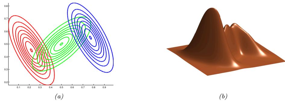
Figure 3.11: A mixture of 3 Gaussians in 2d. (a) We show the contours of constant probability for each component in the mixture. (b) A surface plot of the overall density. Adapted from Figure 2.23 of [Bis06]. Generated by gmm\_plot\_demo.ipynb

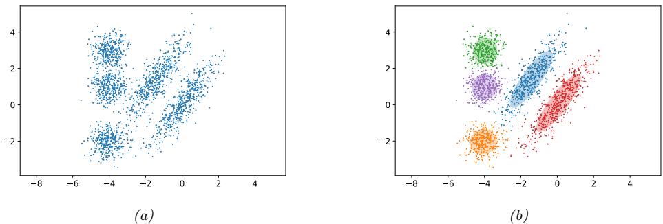
Figure 3.12: (a) Some data in 2d. (b) A possible clustering using K = 5 clusters computed using a GMM. Generated by gmm\_2d.ipynb.

3.5.1 Gaussian mixture models

A Gaussian mixture model or GMM, also called a mixture of Gaussians (MoG), is defined as follows:

\[p(y|\theta) = \sum\_{k=1}^{K} \pi\_k \mathcal{N}(y|\mu\_k, \Sigma\_k) \tag{3.98}\]

In Figure 3.11 we show the density defined by a mixture of 3 Gaussians in 2d. Each mixture component is represented by a di!erent set of elliptical contours. If we let the number of mixture components grow su”ciently large, a GMM can approximate any smooth distribution over R^D.

GMMs are often used for unsupervised clustering of real-valued data samples ^{yn → RD}. This works in two stages. First we fit the model e.g., by computing the MLE ^{ωˆ =} argmax log ^p(D|ω), where

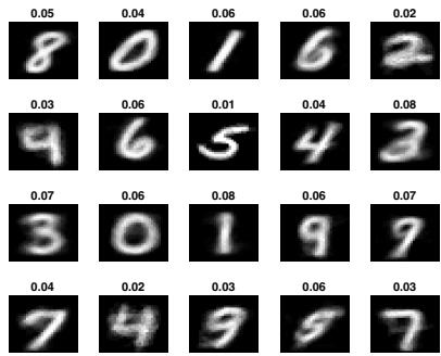
Figure 3.13: We fit a mixture of 20 Bernoullis to the binarized MNIST digit data. We visualize the estimated cluster means µˆk. The numbers on top of each image represent the estimated mixing weights ςˆk. No labels were used when training the model. Generated by mix\_bernoulli\_em\_mnist.ipynb.

D = {yⁿ : n =1: N}. (We discuss how to compute this MLE in Section 8.7.3.) Then we associate each data point yⁿ with a discrete latent or hidden variable zⁿ → {1,…,K} which specifies the identity of the mixture component or cluster which was used to generate yn. These latent identities are unknown, but we can compute a posterior over them using Bayes rule:

\[r\_{nk} \triangleq p(z\_n = k | y\_n, \theta) = \frac{p(z\_n = k | \theta) p(y\_n | z\_n = k, \theta)}{\sum\_{k'=1}^{K} p(z\_n = k' | \theta) p(y\_n | z\_n = k', \theta)} \tag{3.99}\]

The quantity rnk is called the responsibility of cluster k for data point n. Given the responsibilities, we can compute the most probable cluster assignment as follows:

\[\hat{z}\_n = \arg\max\_k r\_{nk} = \arg\max\_k \left[ \log p(\mathbf{y}\_n | z\_n = k, \boldsymbol{\theta}) + \log p(z\_n = k | \boldsymbol{\theta}) \right] \tag{3.100}\]

This is known as hard clustering. (If we use the responsibilities to fractionally assign each data point to di!erent clusters, it is called soft clustering.) See Figure 3.12 for an example.

If we have a uniform prior over zn, and we use spherical Gaussians with !^k = I, the hard clustering problem reduces to

\[z\_n = \underset{k}{\text{argmin}} \, ||\mathfrak{y}\_n - \hat{\mathfrak{m}}\_k||\_2^2 \tag{3.101}\]

In other words, we assign each data point to its closest centroid, as measured by Euclidean distance. This is the basis of the K-means clustering algorithm, which we discuss in Section 21.3.

3.5.2 Bernoulli mixture models

If the data is binary valued, we can use a Bernoulli mixture model or BMM (also called a mixture of Bernoullis), where each mixture component has the following form:

\[p(\mathbf{y}|z=k,\boldsymbol{\theta}) = \prod\_{d=1}^{D} \text{Ber}(y\_d|\mu\_{dk}) = \prod\_{d=1}^{D} \mu\_{dk}^{y\_d} (1-\mu\_{dk})^{1-y\_d} \tag{3.102}\]

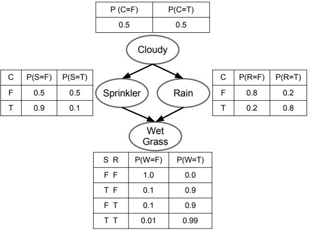
Figure 3.14: Water sprinkler PGM with corresponding binary CPTs. T and F stand for true and false.

Here µdk is the probability that bit d turns on in cluster k.

As an example, we fit a BMM using K = 20 components to the MNIST dataset (Section 3.5.2). (We use the EM algorithm to do this fitting, which is similar to EM for GMMs discussed in Section 8.7.3; however we can also use SGD to fit the model, which is more e”cient for large datasets.3 ) The resulting parameters for each mixture component (i.e., µ^k and ϑk) are shown in Figure 3.13. We see that the model has “discovered” a representation of each type of digit. (Some digits are represented multiple times, since the model does not know the “true” number of classes. See Section 21.3.7 for more information on how to choose the number K of mixture components.)

3.6 Probabilistic graphical models *

I basically know of two principles for treating complicated systems in simple ways: the first is the principle of modularity and the second is the principle of abstraction. I am an apologist for computational probability in machine learning because I believe that probability theory implements these two principles in deep and intriguing ways — namely through factorization and through averaging. Exploiting these two mechanisms as fully as possible seems to me to be the way forward in machine learning. — Michael Jordan, 1997 (quoted in [Fre98]).

We have now introduced a few simple probabilistic building blocks. In Section 3.3, we showed one way to combine some Gaussian building blocks to build a high dimensional distribution p(y) from simpler parts, namely the marginal p(y1) and the conditional p(y2|y1). This idea can be extended to define joint distributions over sets of many random variables. The key assumption we will make is that some variables are conditionally independent of others. We will represent our CI assumptions using graphs, as we briefly explain below. (See the sequel to this book, [Mur23], for more information.)

^3. For the SGD code, see mix\_bernoulli\_sgd\_mnist.ipynb.

3.6.1 Representation

A probabilistic graphical model or PGM is a joint probability distribution that uses a graph structure to encode conditional independence assumptions. When the graph is a directed acyclic graph or DAG, the model is sometimes called a Bayesian network, although there is nothing inherently Bayesian about such models.

The basic idea in PGMs is that each node in the graph represents a random variable, and each edge represents a direct dependency. More precisely, each lack of edge represents a conditional independency. In the DAG case, we can number the nodes in topological order (parents before children), and then we connect them such that each node is conditionally independent of all its predecessors given its parents:

\[Y\_i \perp \mathbf{Y}\_{\text{pred}(i)\backslash\text{pa}(i)} | \mathbf{Y}\_{\text{pa}(i)} \tag{3.103}\]

where pa(i) are the parents of node i, and pred(i) are the predecessors of node i in the ordering. (This is called the ordered Markov property.) Consequently, we can represent the joint distribution as follows:

\[p(\mathbf{Y}\_{1:N\_G}) = \prod\_{i=1}^{N\_G} p(Y\_i | \mathbf{Y}\_{\text{pa}(i)}) \tag{3.104}\]

where N^G is the number of nodes in the graph.

3.6.1.1 Example: water sprinkler network

Suppose we want to model the dependencies between 4 random variables: C (whether it is cloudy season or not), R (whether it is raining or not), S (whether the water sprinkler is on or not), and W (whether the grass is wet or not). We know that the cloudy season makes rain more likely, so we add a C ↔︎ R arc. We know that the cloudy season makes turning on a water sprinkler less likely, so we add a C ↔︎ S arc. Finally, we know that either rain or sprinklers can cause the grass to get wet, so we add S ↔︎ W and R ↔︎ W edges.

Formally, this defines the following joint distribution:

\[p(C, S, R, W) = p(C)p(S|C)p(R|C, S)p(W|S, R, \mathcal{E}')\tag{3.105}\]

where we strike through terms that are not needed due to the conditional independence properties of the model.

Each term p(Yi|Ypa(i)) is a called the conditional probability distribution or CPD for node i. This can be any kind of distribution we like. In Figure 3.14, we assume each CPD is a conditional categorical distribution, which can be represented as a conditional probability table or CPT. We can represent the i’th CPT as follows:

\[\boldsymbol{\theta}\_{ijk} \triangleq p(\boldsymbol{Y}\_i = k | \mathbf{Y}\_{\text{pa}(i)} = j) \tag{3.106}\]

This satisfies the properties ⁰ ↘ ^ϖijk ↘ ¹ and $^{Ki k}=1 ϖijk = 1 for each row j. Here i indexes nodes, i → [NG]; k indexes node states, k → [Ki], where Kⁱ is the number of states for node i; and j indexes joint parent states, ^{j →} [Ji], where ^{Ji = p}↑pa(i) ^Kp. For example, the wet grass node has 2 binary parents, so there are 4 parent states.

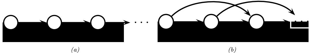
Figure 3.15: Illustration of first and second order autoregressive (Markov) models.

3.6.1.2 Example: Markov chain

Suppose we want to create a joint probability distribution over variable-length sequences, p(y1:^T ). If each variable y^t represents a word from a vocabulary with K possible values, so y^t → {1,…,K}, the resulting model represents a distribution over possible sentences of length T; this is often called a language model.

By the chain rule of probability, we can represent any joint distribution over T variables as follows:

\[p(y\_{1:T}) = p(y\_1)p(y\_2|y\_1)p(y\_3|y\_2, y\_1)p(y\_4|y\_3, y\_2, y\_1) \dots = \prod\_{t=1}^{T} p(y\_t|y\_{1:t-1}) \tag{3.107}\]

Unfortunately, the number of parameters needed to represent each conditional distribution p(yt|y1:t→1) grows exponentially with t. However, suppose we make the conditional independence assumption that the future, yt+1:^T , is independent of the past, y1:t→¹, given the present, yt. This is called the first order Markov condition, and is repesented by the PGM in Figure 3.15(a). With this assumption, we can write the joint distribution as follows:

\[p(y\_{1:T}) = p(y\_1)p(y\_2|y\_1)p(y\_3|y\_2)p(y\_4|y\_3)\dots = p(y\_1)\prod\_{t=2}^{T}p(y\_t|y\_{t-1})\tag{3.108}\]

This is called a Markov chain, Markov model or autoregressive model of order 1.

The function p(yt|y^t→1) is called the transition function, transition kernel or Markov kernel. This is just a conditional distribution over the states at time t given the state at time t ↑ 1, and hence it satisfies the conditions ^p(yt|y^t→¹) ^{∋ 0} and $^{K k}=1 p(y^t = k|y^t→¹ = j)=1. We can represent this CPT as a stochastic matrix, Ajk = p(y^t = k|y^t→¹ = j), where each row sums to 1. This is known as the state transition matrix. We assume this matrix is the same for all time steps, so the model is said to be homogeneous, stationary, or time-invariant. This is an example of parameter tying, since the same parameter is shared by multiple variables. This assumption allows us to model an arbitrary number of variables using a fixed number of parameters.

The first-order Markov assumption is rather strong. Fortunately, we can easily generalize first-order models to depend on the last M observations, thus creating a model of order (memory length) M:

\[p(y\_{1:T}) = p(y\_{1:M}) \prod\_{t=M+1}^{T} p(y\_t|y\_{t-M:t-1}) \tag{3.109}\]

This is called an M’th order Markov model. For example, if M = 2, y^t depends on y^t→¹ and y^t→2, as shown in Figure 3.15(b). This is called a trigram model, since it models the distribution over

word triples. If we use M = 1, we get a bigram model, which models the distribution over word pairs.

For large vocabulary sizes, the number of parameters needed to estimate the conditional distributions for M-gram models for large M can become prohibitive. In this case, we need to make additional assumptions beyond conditional independence. For example, we can assume that p(yt|yt→M:t→1) can be represented as a low-rank matrix, or in terms of some kind of neural network. This is called a neural language model. See Chapter 15 for details.

3.6.2 Inference

A PGM defines a joint probability distribution. We can therefore use the rules of marginalization and conditioning to compute p(Yi|Y^j = y^j ) for any sets of variables i and j. E”cient algorithms to perform this computation are discussed in the sequel to this book, [Mur23].

For example, consider the water sprinkler example in Figure 3.14. Our prior belief that it has rained is given by p(R = 1) = 0.5. If we see that the grass is wet, then our posterior belief that it has rained changes to p(R = 1|W = 1) = 0.7079. Now suppose we also notice the water sprinkler was turned on: our belief that it rained goes down to p(R = 1|W = 1, S = 1) = 0.3204. This negative mutual interaction between multiple causes of some observations is called the explaining away e!ect, also known as Berkson’s paradox. (See sprinkler\_pgm.ipynb for some code that reproduces these calculations.)

3.6.3 Learning

If the parameters of the CPDs are unknown, we can view them as additional random variables, add them as nodes to the graph, and then treat them as hidden variables to be inferred. Figure 3.16(a) shows a simple example, in which we have N iid random variables, yn, all drawn from the same distribution with common parameter ω. (The shaded nodes represent observed values, whereas the unshaded (hollow) nodes represent latent variables or parameters.)

More precisely, the model encodes the following “generative story” about the data:

\[ \theta \sim p(\theta) \tag{3.110} \]

\[y\_n \sim p(y|\theta) \tag{3.111}\]

where p(ω) is some (unspecified) prior over the parameters, and p(y|ω) is some specified likelihood function. The corresponding joint distribution has the form

\[p(\mathcal{D}, \boldsymbol{\theta}) = p(\boldsymbol{\theta}) p(\mathcal{D}|\boldsymbol{\theta}) \tag{3.112}\]

where D = (y1,…, y^N ). By virtue of the iid assumption, the likelihood can be rewritten as follows:

\[p(\mathcal{D}|\boldsymbol{\theta}) = \prod\_{n=1}^{N} p(y\_n|\boldsymbol{\theta}) \tag{3.113}\]

Notice that the order of the data vectors is not important for defining this model, i.e., we can permute the numbering of the leaf nodes in the PGM. When this property holds, we say that the data is exchangeable.

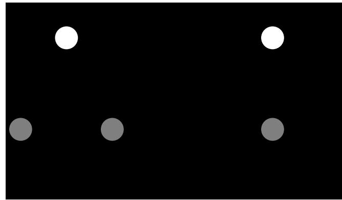
Figure 3.16: Left: data points yⁿ are conditionally independent given ω. Right: Same model, using plate notation. This represents the same model as the one on the left, except the repeated yⁿ nodes are inside a box, known as a plate; the number in the lower right hand corner, N, specifies the number of repetitions of the yⁿ node.

3.6.3.1 Plate notation

In Figure 3.16(a), we see that the y nodes are repeated N times. To avoid visual clutter, it is common to use a form of syntactic sugar called plates. This is a notational convention in which we draw a little box around the repeated variables, with the understanding that nodes within the box will get repeated when the model is unrolled. We often write the number of copies or repetitions in the bottom right corner of the box. This is illustrated in Figure 3.16(b). This notation is widely used to represent certain kinds of Bayesian model.

Figure 3.17 shows a more interesting example, in which we represent a GMM (Section 3.5.1) as a graphical model. We see that this encodes the joint distribution

\[p(\boldsymbol{y}\_{1:N}, \boldsymbol{z}\_{1:N}, \boldsymbol{\theta}) = p(\boldsymbol{\pi}) \left[ \prod\_{k=1}^{K} p(\mu\_k) p(\boldsymbol{\Sigma}\_k) \right] \left[ \prod\_{n=1}^{N} p(z\_n|\boldsymbol{\pi}) p(\boldsymbol{y}\_n|z\_n, \mu\_{1:K}, \boldsymbol{\Sigma}\_{1:K}) \right] \tag{3.114}\]

We see that the latent variables zⁿ as well as the unknown paramters, ω = (ς, µ1:K, !1:K), are all shown as unshaded nodes.

3.7 Exercises

Exercise 3.1 [Uncorrelated does not imply independent † ]

Let ^X ↘ ^U(↑1, 1) and ^{Y = X2}. Clearly ^Y is dependent on ^X (in fact, ^Y is uniquely determined by ^X). However, show that φ(X, Y )=0. Hint: if X ↘ U(a, b) then E[X]=(a + b)/2 and V [X]=(b ↑ a) ²/12.

Exercise 3.2 [Correlation coe!cient is between -1 and +1]

Prove that ↑1 ↗ φ(X, Y ) ↗ 1

Exercise 3.3 [Correlation coe!cient for linearly related variables is ±1 † ] Show that, if Y = aX + b for some parameters a > 0 and b, then φ(X, Y )=1. Similarly show that if a < 0, then φ(X, Y ) = ↑1.

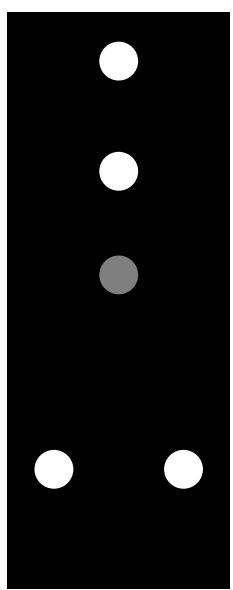
Figure 3.17: A Gaussian mixture model represented as a graphical model.

Exercise 3.4 [Linear combinations of random variables]

Let x be a random vector with mean m and covariance matrix “. Let A and B be matrices.

• 1. Derive the covariance matrix of Ax.
• 2. Show that tr(AB) = tr(BA).
• 3. Derive an expression for E ’ x^T Ax ( .

Exercise 3.5 [Gaussian vs jointly Gaussian ]

Let X ↘ N (0, 1) and Y = W X, where p(W = ↑1) = p(W = 1) = 0.5. It is clear that X and Y are not independent, since Y is a function of X.

• 1. Show Y ↘ N (0, 1).
• 2. Show Cov [X, Y ] = 0. Thus X and Y are uncorrelated but dependent, even though they are Gaussian. Hint: use the definition of covariance

\[\text{Cov}\,[X,Y] = \mathbb{E}\left[XY\right] - \mathbb{E}\left[X\right]\mathbb{E}\left[Y\right] \tag{3.115}\]

and the rule of iterated expectation

\[\mathbb{E}\left[XY\right] = \mathbb{E}\left[\mathbb{E}\left[XY|W\right]\right] \tag{3.116}\]

Exercise 3.6 [Normalization constant for a multidimensional Gaussian]

Prove that the normalization constant for a d-dimensional Gaussian is given by

\[\langle 2\pi \rangle^{d/2} |\boldsymbol{\Sigma}|^{\frac{1}{2}} = \int \exp(-\frac{1}{2}(\boldsymbol{x} - \boldsymbol{\mu})^T \boldsymbol{\Sigma}^{-1} (\boldsymbol{x} - \boldsymbol{\mu})) d\boldsymbol{x} \tag{3.117}\]

Hint: diagonalize ! and use the fact that ^|!^{| =} ) ⁱ ↼ⁱ to write the joint pdf as a product of d one-dimensional Gaussians in a transformed coordinate system. (You will need the change of variables formula.) Finally, use the normalization constant for univariate Gaussians.

Exercise 3.7 [Sensor fusion with known variances in 1d]

Suppose we have two sensors with known (and di”erent) variances v¹ and v2, but unknown (and the same) mean µ. Suppose we observe n¹ observations y(1) ⁱ ↘ N (µ, v1) from the first sensor and n² observations y(2) ⁱ ↘ N (µ, v2) from the second sensor. (For example, suppose µ is the true temperature outside, and sensor 1 is a precise (low variance) digital thermosensing device, and sensor 2 is an imprecise (high variance) mercury thermometer.) Let D represent all the data from both sensors. What is the posterior p(µ|D), assuming a non-informative prior for µ (which we can simulate using a Gaussian with a precision of 0)? Give an explicit expression for the posterior mean and variance.

Exercise 3.8 [Show that the Student distribution can be written as a Gaussian scale mixture]

Show that a Student distribution can be written as a Gaussian scale mixture, where we use a Gamma mixing distribution on the precision ω, i.e.

\[p(x|\mu, a, b) = \int\_0^\infty \mathcal{N}(x|\mu, \alpha^{-1}) \text{Ga}(\alpha|a, b) d\alpha \tag{3.118}\]

This can be viewed as an infinite mixture of Gaussians, with di”erent precisions.

4 Statistics

4.1 Introduction

In Chapter 2–Chapter 3, we assumed all the parameters ω of our probability models were known. In this chapter, we discuss how to learn these parameters from data.

The process of estimating ω from D is called model fitting, or training, and is at the heart of machine learning. There are many methods for producing such estimates, but most boil down to an optimization problem of the form

\[\hat{\theta} = \operatorname\*{argmin}\_{\theta} \mathcal{L}(\theta) \tag{4.1}\]

where L(ω) is some kind of loss function or objective function. We discuss several di!erent loss functions in this chapter. In some cases, we also discuss how to solve the optimization problem in closed form. In general, however, we will need to use some kind of generic optimization algorithm, which we discuss in Chapter 8.

In addition to computing a point estimate, ωˆ, we discuss how to model our uncertainty or confidence in this estimate. In statistics, the process of quantifying uncertainty about an unknown quantity estimated from a finite sample of data is called inference. We will discuss both Bayesian and frequentist approaches to inference.1

4.2 Maximum likelihood estimation (MLE)

The most common approach to parameter estimation is to pick the parameters that assign the highest probability to the training data; this is called maximum likelihood estimation or MLE. We give more details below, and then give a series of worked examples.

4.2.1 Definition

We define the MLE as follows:

\[\hat{\boldsymbol{\theta}}\_{\text{mle}} \triangleq \operatorname\*{argmax}\_{\boldsymbol{\theta}} p(\mathcal{D}|\boldsymbol{\theta}) \tag{4.2}\]

^1. In the deep learning community, the term “inference” refers to what we will call “prediction”, namely computing ^p(y|x, ^ωˆ).

We usually assume the training examples are independently sampled from the same distribution, so the (conditional) likelihood becomes

\[p(\mathcal{D}|\boldsymbol{\theta}) = \prod\_{n=1}^{N} p(y\_n|x\_n, \boldsymbol{\theta})\tag{4.3}\]

This is known as the iid assumption, which stands for “independent and identically distributed”. We usually work with the log likelihood, which is given by

\[\ell(\boldsymbol{\theta}) \triangleq \log p(\mathcal{D}|\boldsymbol{\theta}) = \sum\_{n=1}^{N} \log p(y\_n|x\_n, \boldsymbol{\theta}) \tag{4.4}\]

This decomposes into a sum of terms, one per example. Thus the MLE is given by

\[\hat{\theta}\_{\text{mle}} = \underset{\theta}{\text{argmax}} \sum\_{n=1}^{N} \log p(y\_n | x\_n, \theta) \tag{4.5}\]

Since most optimization algorithms (such as those discussed in Chapter 8) are designed to minimize cost functions, we can redefine the objective function to be the (conditional) negative log likelihood or NLL:

\[\text{NLL}(\boldsymbol{\theta}) \triangleq -\log p(\mathcal{D}|\boldsymbol{\theta}) = -\sum\_{n=1}^{N} \log p(y\_n|\mathbf{x}\_n, \boldsymbol{\theta}) \tag{4.6}\]

Minimizing this will give the MLE. If the model is unconditional (unsupervised), the MLE becomes

\[\hat{\theta}\_{\text{mle}} = \underset{\theta}{\text{argmin}} - \sum\_{n=1}^{N} \log p(y\_n|\theta) \tag{4.7}\]

since we have outputs yⁿ but no inputs xn. 2

Alternatively we may want to maximize the joint likelihood of inputs and outputs. The MLE in this case becomes

\[\hat{\theta}\_{\text{mle}} = \underset{\theta}{\text{argmin}} - \sum\_{n=1}^{N} \log p(y\_n, x\_n | \theta) \tag{4.8}\]

4.2.2 Justification for MLE

There are several ways to justify the method of MLE. One way is to view it as simple point approximation to the Bayesian posterior p(ω|D) using a uniform prior, as explained in Section 4.6.7.1.

^2. In statistics, it is standard to use y to represent variables whose generative distribution we choose to model, and to use x to represent exogenous inputs which are given but not generated. Thus supervised learning concerns fitting conditional models of the form p(y|x), and unsupervised learning is the special case where x = ↑, so we are just fitting the unconditional distribution p(y). In the ML literature, supervised learning treats y as generated and x as given, but in the unsupervised case, it often switches to using x to represent generated variables.

In particular, suppose we approximate the posterior by a delta function, ^p(ω|D) = ↽(^{ω ↑}ωˆmap), where ωˆmap is the posterior mode, given by

\[\hat{\theta}\_{\text{map}} = \underset{\theta}{\text{argmax}} \log p(\theta | \mathcal{D}) = \underset{\theta}{\text{argmax}} \log p(\mathcal{D} | \theta) + \log p(\theta) \tag{4.9}\]

If we use a uniform prior, ^p(ω) ^{∞ 1}, the MAP estimate becomes equal to the MLE, ^ωˆmap ^{= ω}ˆmle.

Another way to justify the use of the MLE is that the resulting predictive distribution ^p(y|ωˆmle) is as close as possible (in a sense to be defined below) to the empirical distribution of the data. In the unconditional case, the empirical distribution is defined by

\[p\_{\mathcal{D}}(\boldsymbol{y}) \triangleq \frac{1}{N} \sum\_{n=1}^{N} \delta(\boldsymbol{y} - \boldsymbol{y}\_{n}) \tag{4.10}\]

We see that the empirical distribution is a series of delta functions or “spikes” at the observed training points. We want to create a model whose distribution q(y) = p(y|ω) is similar to pD(y).

A standard way to measure the (dis)similarity between probability distributions p and q is the Kullback Leibler divergence, or KL divergence. We give the details in Section 6.2, but in brief this is defined as

\[D\_{\text{KL}}\left(p \parallel q\right) = \sum\_{\mathbf{y}} p(\mathbf{y}) \log \frac{p(\mathbf{y})}{q(\mathbf{y})} \tag{4.11}\]

\[=\underbrace{\sum\_{\mathbf{y}}p(\mathbf{y})\log p(\mathbf{y})-\sum\_{\mathbf{y}}p(\mathbf{y})\log q(\mathbf{y})}\_{-\mathbb{H}(p)}\tag{4.12}\]

where H (p) is the entropy of p (see Section 6.1), and Hce (p, q) is the cross-entropy of p and q (see Section 6.1.2). One can show that DKL (p 7 q) ∋ 0, with equality i! p = q.

If we define q(y) = p(y|ω), and set p(y) = pD(y), then the KL divergence becomes

\[D\_{\mathbb{KL}}\left(p \parallel q\right) = \sum\_{\mathbf{y}} \left[p\_{\mathcal{D}}(\mathbf{y}) \log p\_{\mathcal{D}}(\mathbf{y}) - p\_{\mathcal{D}}(\mathbf{y}) \log q(\mathbf{y})\right] \tag{4.13}\]

\[\varepsilon = -\mathbb{H}(p\_{\mathcal{D}}) - \frac{1}{N} \sum\_{n=1}^{N} \log p(y\_n|\theta) \tag{4.14}\]

\[\mathbf{x} = \text{const} + \text{NLL}(\boldsymbol{\theta}) \tag{4.15}\]

The first term is a constant which we can ignore, leaving just the NLL. Thus minimizing the KL is equivalent to minimizing the NLL which is equivalent to computing the MLE, as in Equation (4.7).

We can generalize the above results to the supervised (conditional) setting by using the following empirical distribution:

\[p\_{\mathcal{D}}(\boldsymbol{x}, \boldsymbol{y}) = p\_{\mathcal{D}}(\boldsymbol{y}|\boldsymbol{x}) p\_{\mathcal{D}}(\boldsymbol{x}) = \frac{1}{N} \sum\_{n=1}^{N} \delta(\boldsymbol{x} - \boldsymbol{x}\_{n}) \delta(\boldsymbol{y} - \boldsymbol{y}\_{n}) \tag{4.16}\]

The expected KL then becomes

\[\mathbb{E}\_{p\_{\mathcal{D}}(\mathbf{z})} \left[ D\_{\text{KL}}(p\_{\mathcal{D}}(Y|x) \parallel q(Y|x)) \right] = \sum\_{\mathbf{z}} p\_{\mathcal{D}}(\mathbf{z}) \left[ \sum\_{\mathbf{y}} p\_{\mathcal{D}}(\mathbf{y}|x) \log \frac{p\_{\mathcal{D}}(\mathbf{y}|x)}{q(\mathbf{y}|x)} \right] \tag{4.17}\]

\[=\text{const} - \sum\_{\mathfrak{w},\mathfrak{y}} p\_{\mathcal{D}}(\mathfrak{x},\mathfrak{y}) \log q(\mathfrak{y}|\mathfrak{x}) \tag{4.18}\]

\[=\text{const} - \frac{1}{N} \sum\_{n=1}^{N} \log p(y\_n | x\_n, \theta) \tag{4.19}\]

Minimizing this is equivalent to minimizing the conditional NLL in Equation (4.6).

4.2.3 Example: MLE for the Bernoulli distribution

Suppose Y is a random variable representing a coin toss, where the event Y = 1 corresponds to heads and Y = 0 corresponds to tails. Let ϖ = p(Y = 1) be the probability of heads. The probability distribution for this rv is the Bernoulli, which we introduced in Section 2.4.

The NLL for the Bernoulli distribution is given by

\[\text{NLL}(\theta) = -\log \prod\_{n=1}^{N} p(y\_n|\theta) \tag{4.20}\]

\[\hat{\theta} = -\log \prod\_{n=1}^{N} \theta^{\mathbb{I}(y\_n=1)} (1-\theta)^{\mathbb{I}(y\_n=0)} \tag{4.21}\]

\[=-\sum\_{n=1}^{N} \left[ \mathbb{I}\left(y\_n = 1\right) \log \theta + \mathbb{I}\left(y\_n = 0\right) \log(1 - \theta) \right] \tag{4.22}\]

\[=-\left[N\_1 \log \theta + N\_0 \log(1-\theta)\right] \tag{4.23}\]

where we have defined N¹ = $^{N n}=1 ^I(yⁿ = 1) and ^{N0 =} $^{N n}=1 I(yⁿ = 0), representing the number of heads and tails. (The NLL for the binomial is the same as for the Bernoulli, modulo an irrelevant .^N c / term, which is a constant independent of ϖ.) These two numbers are called the su!cient statistics of the data, since they summarize everything we need to know about D. The total count, N = N⁰ + N1, is called the sample size.

The MLE can be found by solving ^{d d}ϱNLL(ϖ)=0. The derivative of the NLL is

\[\frac{d}{d\theta} \text{NLL}(\theta) = \frac{-N\_1}{\theta} + \frac{N\_0}{1 - \theta} \tag{4.24}\]

and hence the MLE is given by

\[\hat{\theta}\_{\text{mle}} = \frac{N\_1}{N\_0 + N\_1} \tag{4.25}\]

We see that this is just the empirical fraction of heads, which is an intuitive result.

4.2.4 Example: MLE for the categorical distribution

Suppose we roll a K-sided dice N times. Let Yⁿ → {1,…,K} be the n’th outcome, where Yⁿ ⇒ Cat(ω). We want to estimate the probabilities ω from the dataset D = {yⁿ : n =1: N}. The NLL is given by

\[\text{NLL}(\boldsymbol{\theta}) = -\sum\_{k} N\_{k} \log \theta\_{k} \tag{4.26}\]

where N^k is the number of times the event Y = k is observed. (The NLL for the multinomial is the same, up to irrelevant scale factors.)

To compute the MLE, we have to minimize the NLL subject to the constraint that $^{K k}=1 ϖ^k = 1. To do this, we will use the method of Lagrange multipliers (see Section 8.5.1).3

The Lagrangian is as follows:

\[\mathcal{L}(\boldsymbol{\theta},\lambda) \triangleq -\sum\_{k} N\_{k} \log \theta\_{k} - \lambda \left(1 - \sum\_{k} \theta\_{k}\right) \tag{4.27}\]

Taking derivatives with respect to φ yields the original constraint:

\[\frac{\partial \mathcal{L}}{\partial \lambda} = 1 - \sum\_{k} \theta\_{k} = 0 \tag{4.28}\]

Taking derivatives with respect to ϖ^k yields

\[\frac{\partial \mathcal{L}}{\partial \theta\_k} = -\frac{N\_k}{\theta\_k} + \lambda = 0 \implies N\_k = \lambda \theta\_k \tag{4.29}\]

We can solve for φ using the sum-to-one constraint:

\[\sum\_{k} N\_{k} = N = \lambda \sum\_{k} \theta\_{k} = \lambda \tag{4.30}\]

Thus the MLE is given by

\[ \hat{\theta}\_k = \frac{N\_k}{\lambda} = \frac{N\_k}{N} \tag{4.31} \]

which is just the empirical fraction of times event k occurs.

4.2.5 Example: MLE for the univariate Gaussian

Suppose ^{Y ⇒ N} (µ, ^ε2) and let ^D = {yⁿ : ⁿ =1: ^N} be an iid sample of size ^N. We can estimate the parameters ω = (µ, ε²) using MLE as follows. First, we derive the NLL, which is given by

\[\text{NLL}(\mu, \sigma^2) = -\sum\_{n=1}^{N} \log \left[ \left( \frac{1}{2\pi\sigma^2} \right)^{\frac{1}{2}} \exp \left( -\frac{1}{2\sigma^2} (y\_n - \mu)^2 \right) \right] \tag{4.32}\]

\[\hat{\sigma} = \frac{1}{2\sigma^2} \sum\_{n=1}^{N} (y\_n - \mu)^2 + \frac{N}{2} \log(2\pi\sigma^2) \tag{4.33}\]

^3. We do not need to explicitly enforce the constraint that ε^k ↓ 0 since the gradient of the Lagrangian has the form ↔︎Nk/ε^k ↔︎ ϑ; so negative values of ε^k would increase the objective, rather than minimize it. (Of course, this does not preclude setting ε^k = 0, and indeed this is the optimal solution if N^k = 0.)

The minimum of this function must satisfy the following conditions, which we explain in Section 8.1.1.1:

\[\frac{\partial}{\partial \mu} \text{NLL}(\mu, \sigma^2) = 0, \ \frac{\partial}{\partial \sigma^2} \text{NLL}(\mu, \sigma^2) = 0 \tag{4.34}\]

So all we have to do is to find this stationary point. Some simple calculus (Exercise 4.1) shows that the solution is given by the following:

\[ \hat{\mu}\_{\text{mle}} = \frac{1}{N} \sum\_{n=1}^{N} y\_n = \overline{y} \tag{4.35} \]

\[\hat{\sigma}\_{\text{mle}}^2 = \frac{1}{N} \sum\_{n=1}^N (y\_n - \hat{\mu}\_{\text{mle}})^2 = \frac{1}{N} \sum\_{n=1}^N \left[ y\_n^2 + \hat{\mu}\_{\text{mle}}^2 - 2y\_n \hat{\mu}\_{\text{mle}} \right] = s^2 - \overline{y}^2 \tag{4.36}\]

\[s^2 \triangleq \frac{1}{N} \sum\_{n=1}^{N} y\_n^2 \tag{4.37}\]

The quantities y and s² are called the su!cient statistics of the data, since they are su”cient to compute the MLE, without loss of information relative to using the raw data itself.

Note that you might be used to seeing the estimate for the variance written as

\[ \hat{\sigma}\_{\text{unb}}^2 = \frac{1}{N-1} \sum\_{n=1}^N (y\_n - \hat{\mu}\_{\text{mle}})^2 \tag{4.38} \]

where we divide by N ↑ 1. This is not the MLE, but is a di!erent kind of estimate, which happens to be unbiased (unlike the MLE); see Section 4.7.6.1 for details.4

4.2.6 Example: MLE for the multivariate Gaussian

In this section, we derive the maximum likelihood estimate for the parameters of a multivariate Gaussian.

First, let us write the log-likelihood, dropping irrelevant constants:

\[\ell(\mu, \Sigma) = \log p(\mathcal{D} | \mu, \Sigma) = \frac{N}{2} \log |\Lambda| - \frac{1}{2} \sum\_{n=1}^{N} (y\_n - \mu)^{\mathsf{T}} \Lambda (y\_n - \mu) \tag{4.39}\]

where ” = !^→1 is the precision matrix (inverse covariance matrix).

^4. Note that, in Python, numpy defaults to the MLE, but Pandas defaults to the unbiased estimate, as explained in https://stackoverflow.com/questions/24984178/different-std-in-pandas-vs-numpy/.

4.2.6.1 MLE for the mean

Using the substitution zⁿ = yⁿ ↑ µ, the derivative of a quadratic form (Equation (7.264)) and the chain rule of calculus, we have

\[\frac{\partial}{\partial \mu} (y\_n - \mu)^\mathsf{T} \Sigma^{-1} (y\_n - \mu) = \frac{\partial}{\partial \mathbf{z}\_n} \mathbf{z}\_n^\mathsf{T} \Sigma^{-1} \mathbf{z}\_n \frac{\partial \mathbf{z}\_n}{\partial \mu^\mathsf{T}} \tag{4.40}\]

\[\mathbf{z} = -\mathbf{1}(\boldsymbol{\Sigma}^{-1} + \boldsymbol{\Sigma}^{-T})\mathbf{z}\_n \tag{4.41}\]

since ^ϖz^{n ϖ}µ^T = ↑I. Hence

\[\frac{\partial}{\partial \mu} \ell(\mu, \Sigma) = -\frac{1}{2} \sum\_{n=1}^{N} -2\Sigma^{-1} (y\_n - \mu) = \Sigma^{-1} \sum\_{n=1}^{N} (y\_n - \mu) = 0 \tag{4.42}\]

\[ \hat{\mu} = \frac{1}{N} \sum\_{n=1}^{N} y\_n = \overline{y} \tag{4.43} \]

So the MLE of µ is just the empirical mean.

4.2.6.2 MLE for the covariance matrix

We can use the trace trick (Equation (7.36)) to rewrite the log-likelihood in terms of the precision matrix ” = !^→1 as follows:

\[\ell(\hat{\mu}, \Lambda) = \frac{N}{2} \log |\Lambda| - \frac{1}{2} \sum\_{n} \text{tr} [(y\_n - \hat{\mu})(y\_n - \hat{\mu})^\mathsf{T} \Lambda] \tag{4.44}\]

\[\mathbf{E} = \frac{N}{2} \log |\mathbf{A}| - \frac{1}{2} \text{tr} \left[ \mathbf{S}\_{\overline{\mathbf{y}}} \mathbf{A} \right] \tag{4.45}\]

\[\mathbf{S}\_{\overline{\mathbf{y}}} \triangleq \sum\_{n=1}^{N} (y\_n - \overline{y})(y\_n - \overline{y})^\top = \left(\sum\_n y\_n y\_n^\top\right) - N\overline{y}\overline{y}^\top \tag{4.46}\]

where S^y is the scatter matrix centered on y.

We can rewrite the scatter matrix in a more compact form as follows:

\[\mathbf{S}\_{\overline{\mathbf{y}}} = \hat{\mathbf{Y}}^{\mathsf{T}} \hat{\mathbf{Y}} = \mathbf{Y}^{\mathsf{T}} \mathbf{C}\_{N}^{\mathsf{T}} \mathbf{C}\_{N} \mathbf{Y} = \mathbf{Y}^{\mathsf{T}} \mathbf{C}\_{N} \mathbf{Y} \tag{4.47}\]

where

\[\mathbf{C}\_{N} \triangleq \mathbf{I}\_{N} - \frac{1}{N} \mathbf{1}\_{N} \mathbf{1}\_{N}^{\mathsf{T}} \tag{4.48}\]

is the centering matrix, which converts Y to Y˜ by subtracting the mean y = ^{1 N} Y^T1^N o! every row.

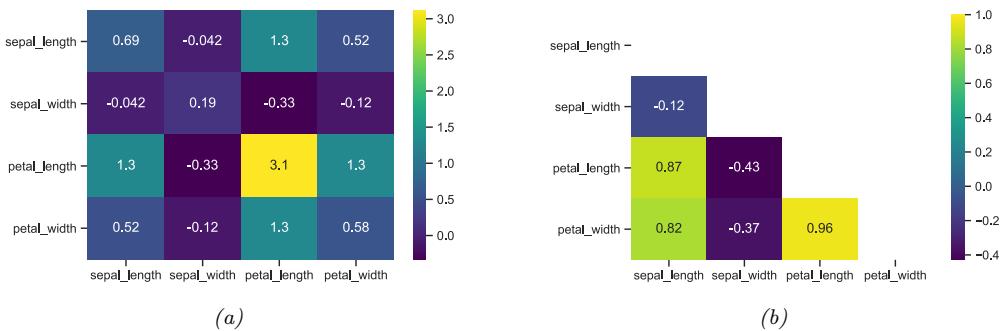
Figure 4.1: (a) Covariance matrix for the features in the iris dataset from Section 1.2.1.1. (b) Correlation matrix. We only show the lower triangle, since the matrix is symmetric and has a unit diagonal. Compare this to Figure 1.3. Generated by iris\_cov\_mat.ipynb.

Using results from Section 7.8, we can compute derivatives of the loss with respect to ” to get

\[\frac{\partial \ell(\hat{\mu}, \Lambda)}{\partial \Lambda} = \frac{N}{2} \Lambda^{-T} - \frac{1}{2} \mathbf{S}\_{\overline{\Psi}}^{\overline{\r}} = \mathbf{0} \tag{4.49}\]

\[ \mathbf{A}^{-\mathsf{T}} = \mathbf{A}^{-1} = \boldsymbol{\Sigma} = \frac{1}{N} \mathbf{S}\_{\overline{\mathsf{Y}}} \tag{4.50} \]

\[\hat{\Sigma} = \frac{1}{N} \sum\_{n=1}^{N} (y\_n - \overline{y})(y\_n - \overline{y})^\top = \frac{1}{N} \mathbf{Y}^\top \mathbf{C}\_N \mathbf{Y} \tag{4.51}\]

Thus the MLE for the covariance matrix is the empirical covariance matrix. See Figure 4.1a for an example.

Sometimes it is more convenient to work with the correlation matrix defined in Equation (3.8). This can be computed using

\[\text{corr}(\mathbf{Y}) = (\text{diag}(\boldsymbol{\Sigma}))^{-\frac{1}{2}} \boldsymbol{\Sigma} \left(\text{diag}(\boldsymbol{\Sigma})\right)^{-\frac{1}{2}} \tag{4.52}\]

where diag(!)^{→ 1 2} is a diagonal matrix containing the entries 1/εi. See Figure 4.1b for an example.

Note, however, that the MLE may overfit or be numerically unstable, especially when the number of samples N is small compared to the number of dimensions D. The main problem is that ! has O(D²) parameters, so we may need a lot of data to reliably estimate it. In particular, as we see from Equation (4.51), the MLE for a full covariance matrix is singular if N<D. And even when N>D, the MLE can be ill-conditioned, meaning it is close to singular. We discuss solutions to this problem in Section 4.5.2.

4.2.7 Example: MLE for linear regression

We briefly mentioned linear regression in Section 2.6.3. Recall that it corresponds to the following model:

\[p(y|x; \theta) = \mathcal{N}(y|w^\top x, \sigma^2) \tag{4.53}\]

where ω = (w, ε2). Let us assume for now that ε² is fixed, and focus on estimating the weights w. The negative log likelihood or NLL is given by

\[\text{NLL}(\boldsymbol{w}) = -\sum\_{n=1}^{N} \log \left[ \left( \frac{1}{2\pi\sigma^2} \right)^{\frac{1}{2}} \exp \left( -\frac{1}{2\sigma^2} (y\_n - \boldsymbol{w}^\mathsf{T}\boldsymbol{x}\_n)^2 \right) \right] \tag{4.54}\]

Dropping the irrelevant additive constants gives the following simplified objective, known as the residual sum of squares or RSS:

\[\text{RSS}(\mathbf{w}) \triangleq \sum\_{n=1}^{N} (y\_n - \mathbf{w}^\mathsf{T} \mathbf{x}\_n)^2 = \sum\_{n=1}^{N} r\_n^2 \tag{4.55}\]

where rⁿ the n’th residual error. Scaling by the number of examples N gives the mean squared error or MSE:

\[\text{MSE}(\boldsymbol{w}) = \frac{1}{N} \text{RSS}(\boldsymbol{w}) = \frac{1}{N} \sum\_{n=1}^{N} (y\_n - \boldsymbol{w}^\mathsf{T} \boldsymbol{x}\_n)^2 \tag{4.56}\]

Finally, taking the square root gives the root mean squared error or RMSE:

\[\text{RMSE}(\boldsymbol{w}) = \sqrt{\text{MSE}(\boldsymbol{w})} = \sqrt{\frac{1}{N} \sum\_{n=1}^{N} (y\_n - \boldsymbol{w}^\mathrm{T} \boldsymbol{x}\_n)^2} \tag{4.57}\]

We can compute the MLE by minimizing the NLL, RSS, MSE or RMSE. All will give the same results, since these objective functions are all the same, up to irrelevant constants

Let us focus on the RSS objective. It can be written in matrix notation as follows:

\[\text{RSS}(w) = \sum\_{n=1}^{N} (y\_n - \mathbf{w}^\top x\_n)^2 = ||\mathbf{X}w - y||\_2^2 = (\mathbf{X}w - y)^\top (\mathbf{X}w - y) \tag{4.58}\]

In Section 11.2.2.1, we prove that the optimum, which occurs where ̸wRSS(w) = 0, satisfies the following equation:

\[\hat{\boldsymbol{w}}\_{\text{mle}} \triangleq \operatorname\*{argmin}\_{\mathbf{w}} \text{RSS}(\boldsymbol{w}) = (\mathbf{X}^{\mathsf{T}} \mathbf{X})^{-1} \mathbf{X}^{\mathsf{T}} \boldsymbol{y} \tag{4.59}\]

This is called the ordinary least squares or OLS estimate, and is equivalent to the MLE.

4.3 Empirical risk minimization (ERM)

We can generalize MLE by replacing the (conditional) log loss term in Equation (4.6), ω(yn, ω; xn) = ↑ log p(yn|xn, ω), with any other loss function, to get

\[\mathcal{L}(\boldsymbol{\theta}) = \frac{1}{N} \sum\_{n=1}^{N} \ell(y\_n, \boldsymbol{\theta}; x\_n) \tag{4.60}\]

This is known as empirical risk minimization or ERM, since it is the expected loss where the expectation is taken wrt the empirical distribution. See Section 5.4 for more details.

4.3.1 Example: minimizing the misclassification rate

If we are solving a classification problem, we might want to use 0-1 loss:

\[\ell\_{01}(y\_n, \theta; x\_n) = \begin{cases} 0 & \text{if } y\_n = f(x\_n; \theta) \\ 1 & \text{if } y\_n \neq f(x\_n; \theta) \end{cases} \tag{4.61}\]

where f(x; ω) is some kind of predictor. The empirical risk becomes

\[\mathcal{L}(\boldsymbol{\theta}) = \frac{1}{N} \sum\_{n=1}^{N} \ell\_{01}(y\_n, \boldsymbol{\theta}; \boldsymbol{x}\_n) \tag{4.62}\]

This is just the empirical misclassification rate on the training set.

Note that for binary problems, we can rewrite the misclassifcation rate in the following notation. Let y˜ → {↑1, +1} be the true label, and yˆ → {↑1, +1} = f(x; ω) be our prediction. We define the 0-1 loss as follows:

\[\ell\_{01}(\ddot{y}, \hat{y}) = \mathbb{I}\left(\ddot{y} \neq \hat{y}\right) = \mathbb{I}\left(\ddot{y} \,\hat{y} < 0\right) \tag{4.63}\]

The corresponding empirical risk becomes

\[\mathcal{L}(\boldsymbol{\theta}) = \frac{1}{N} \sum\_{n=1}^{N} \ell\_{01}(y\_n, \hat{y}\_n) = \frac{1}{N} \sum\_{n=1}^{N} \mathbb{I}\left(\hat{y}\_n \,\,\hat{y}\_n < 0\right) \tag{4.64}\]

where the dependence on xⁿ and ω is implicit.

4.3.2 Surrogate loss

Unfortunately, the 0-1 loss used in Section 4.3.1 is a non-smooth step function, as shown in Figure 4.2, making it di”cult to optimize. (In fact, it is NP-hard [BDEL03].) In this section we consider the use of a surrogate loss function [BJM06]. The surrogate is usually chosen to be a maximally tight convex upper bound, which is then easy to minimize.

For example, consider a probabilistic binary classifier, which produces the following distribution over labels:

\[p(\ddot{y}|x,\theta) = \sigma(\ddot{y}\eta) = \frac{1}{1 + e^{-\ddot{y}\eta}}\tag{4.65}\]

where ◁ = f(x; ω) is the log odds. Hence the log loss is given by

\[\ell\_{ll}(\ddot{y}, \eta) = -\log p(\ddot{y}|\eta) = \log(1 + e^{-\ddagger \eta}) \tag{4.66}\]

Figure 4.2 shows that this is a smooth upper bound to the 0-1 loss, where we plot the loss vs the quantity y˜◁, known as the margin, since it defines a “margin of safety” away from the threshold value of 0. Thus we see that minimizing the negative log likelihood is equivalent to minimizing a (fairly tight) upper bound on the empirical 0-1 loss.

Another convex upper bound to 0-1 loss is the hinge loss, which is defined as follows:

\[\ell\_{\text{hinge}}(\ddot{y}, \eta) = \max(0, 1 - \ddot{y}\eta) \stackrel{\Delta}{=} (1 - \ddot{y}\eta)\_{+} \tag{4.67}\]

This is plotted in Figure 4.2; we see that it has the shape of a partially open door hinge. This is convex upper bound to the 0-1 loss, although it is only piecewise di!erentiable, not everywhere di!erentiable.

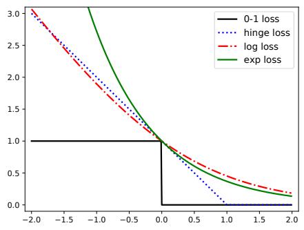
Figure 4.2: Illustration of various loss functions for binary classification. The horizontal axis is the margin ^{z = y}˜↽, the vertical axis is the loss. 0-1 loss is ^I(z < 0). Hinge-loss is max(0, ¹↑z). Log-loss is log2(1 +e→^z). Exp-loss is e→^z. Generated by hinge\_loss\_plot.ipynb.

4.4 Other estimation methods *

4.4.1 The method of moments

Computing the MLE requires solving the equation ̸ωNLL(ω) = 0. Sometimes this is computationally di”cult. In such cases, we may be able to use a simpler approach known as the method of moments (MOM). In this approach, we equate the theoretical moments of the distribution to the empirical moments, and solve the resulting set of K simultaneous equations, where K is the number of parameters. The theoretical moments are given by µ^k = E + Y ^k, , for k =1: K, and the empirical moments are given by

\[ \hat{\mu}\_k = \frac{1}{N} \sum\_{n=1}^n y\_n^k \tag{4.68} \]

so we just need to solve µ^k = ˆµ^k for each k. We give some examples below.

The method of moments is simple, but it is theoretically inferior to the MLE approach, since it may not use all the data as e”ciently. (For details on these theoretical results, see e.g., [CB02].) Furthermore, it can sometimes produce inconsistent results (see Section 4.4.1.2). However, when it produces valid estimates, it can be used to initialize iterative algorithms that are used to optimize the NLL (see e.g., [AHK12]), thus combining the computational e”ciency of MOM with the statistical accuracy of MLE.

4.4.1.1 Example: MOM for the univariate Gaussian

For example, consider the case of a univariate Gaussian distribution. From Section 4.2.5, we have

\[ \mu\_1 = \mu = \overline{y} \tag{4.69} \]

\[ \mu\_2 = \sigma^2 + \mu^2 = s^2 \tag{4.70} \]

where y is the empirical mean and s² is the empirical average sum of squares. so µˆ = y and ^εˆ^{2 = s2 ↑ y2}. In this case, the MOM estimate is the same as the MLE, but this is not always the case.

4.4.1.2 Example: MOM for the uniform distribution

In this section, we give an example of the MOM applied to the uniform distribution. Our presentation follows the wikipedia page.5 Let ^{Y ⇒} Unif(ϖ1, ^ϖ2) be a uniform random variable, so

\[p(y|\theta) = \frac{1}{\theta\_2 - \theta\_1} \mathbb{I}\left(\theta\_1 \le y \le \theta\_2\right) \tag{4.71}\]

The first two moments are

\[\mu\_1 = \mathbb{E}\left[Y\right] = \frac{1}{2}(\theta\_1 + \theta\_2) \tag{4.72}\]

\[\mu\_2 = \mathbb{E}\left[Y^2\right] = \frac{1}{3}(\theta\_1^2 + \theta\_1\theta\_2 + \theta\_2^2) \tag{4.73}\]

Inverting these equations gives

\[\rho\_1(\theta\_1, \theta\_2) = \left(\mu\_1 - \sqrt{3(\mu\_2 - \mu\_1^2)}, 2\mu\_1 - \theta\_1\right) \tag{4.74}\]

Unfortunately this estimator can sometimes give invalid results. For example, suppose D = {0, ⁰, ⁰, ⁰, ¹}. The empirical moments are ^µˆ^{1 = 1 5} and ^µˆ² = ^{1 5} , so the estimated parameters are ˆϖ¹ = ^{1 5 ↑ 2} ⇐3 ^{5 = ↑}0.⁴⁹³ and ^ˆϖ^{2 = 1 5} + ² ⇐3 ⁵ = 0.893. However, these cannot possibly be the correct parameters, since if ϖ² = 0.893, we cannot generate a sample as large as 1.

By contrast, consider the MLE. Let y(1) ↘ y(2) ↘ ··· ↘ y(N) be the order statistics of the data (i.e., the values sorted in increasing order). Let ϖ = ϖ² ↑ ϖ1. Then the likelihood is given by

\[p(\mathcal{D}|\theta) = (\theta)^{-N} \mathbb{1} \left( y\_{(1)} \ge \theta\_1 \right) \mathbb{1} \left( y\_{(N)} \le \theta\_2 \right) \tag{4.75}\]

Within the permitted bounds for ϖ, the derivative of the log likelihood is given by

\[\frac{d}{d\theta}\log p(\mathcal{D}|\theta) = -\frac{N}{\theta} < 0\tag{4.76}\]

Hence the likelihood is a decreasing function of ϖ, so we should pick

\[ \hat{\theta}\_1 = y\_{(1)}, \hat{\theta}\_2 = y\_{(N)} \tag{4.77} \]

In the above example, we get ˆϖ¹ = 0 and ˆϖ² = 1, as one would expect.

^5. https://en.wikipedia.org/wiki/Method\_of\moments\(statistics).

4.4.2 Online (recursive) estimation

If the entire dataset D is available before training starts, we say that we are doing batch learning. However, in some cases, the data set arrives sequentially, so D = {y1, y2,…} in an unbounded stream. In this case, we want to perform online learning.

Let ^ωˆt→¹ be our estimate (e.g., MLE) given ^D1:t→1. To ensure our learning algorithm takes constant time per update, we need to find a learning rule of the form

\[\theta\_t = f(\hat{\theta}\_{t-1}, y\_t) \tag{4.78}\]

This is called a recursive update. Below we give some examples of such online learning methods.

4.4.2.1 Example: recursive MLE for the mean of a Gaussian

Let us reconsider the example from Section 4.2.5 where we computed the MLE for a univariate Gaussian. We know that the batch estimate for the mean is given by

\[ \hat{\mu}\_t = \frac{1}{t} \sum\_{n=1}^t \mathbf{y}\_n \tag{4.79} \]

This is just a running sum of the data, so we can easily convert this into a recursive estimate as follows:

\[ \hat{\mu}\_t = \frac{1}{t} \sum\_{n=1}^t \mathbf{y}\_n = \frac{1}{t} \left( (t-1)\hat{\mu}\_{t-1} + \mathbf{y}\_t \right) \tag{4.80} \]

\[ \hat{\mu}\_t = \hat{\mu}\_{t-1} + \frac{1}{t}(y\_t - \hat{\mu}\_{t-1}) \tag{4.81} \]

This is known as a moving average.

We see from Equation (4.81) that the new estimate is the old estimate plus a correction term. The size of the correction diminishes over time (i.e., as we get more samples). However, if the distribution is changing, we want to give more weight to more recent data examples. We discuss how to do this in Section 4.4.2.2.

4.4.2.2 Exponentially-weighted moving average

Equation (4.81) shows how to compute the moving average of a signal. In this section, we show how to adjust this to give more weight to more recent examples. In particular, we will compute the following exponentially weighted moving average or EWMA, also called an exponential moving average or EMA:

\[ \hat{\mu}\_t = \beta \mu\_{t-1} + (1 - \beta) y\_t \tag{4.82} \]

where 0 ^&lt; ^{1 &}lt; 1. The contribution of a data point ^k steps in the past is weighted by ^1k(1 ^{↑ 1}). Thus the contribution from old data is exponentially decreasing. In particular, we have

\[ \hat{\mu}\_t = \beta \mu\_{t-1} + (1 - \beta) y\_t \tag{4.83} \]

\[\dot{\mathbf{y}} = \beta^2 \mu\_{t-2} + \beta(1-\beta)\mathbf{y}\_{t-1} + (1-\beta)\mathbf{y}\_t \tag{4.84}\]

\[\mathbf{y} = \beta^t \mathbf{y}\_0 + (1 - \beta)\beta^{t-1} \mathbf{y}\_1 + \dots + (1 - \beta)\beta \mathbf{y}\_{t-1} + (1 - \beta)\mathbf{y}\_t \tag{4.85}\]

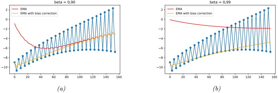
Figure 4.3: Illustration of exponentially-weighted moving average with and without bias correction. (a) Short memory: ⇀ = 0.9. (a) Long memory: ⇀ = 0.99. Generated by ema\_demo.ipynb.

The sum of a geometric series is given by

\[ \beta^t + \beta^{t-1} + \dots + \beta^1 + \beta^0 = \frac{1 - \beta^{t+1}}{1 - \beta} \tag{4.86} \]

Hence

\[(1 - \beta) \sum\_{k=0}^{t} \beta^k = (1 - \beta) \frac{1 - \beta^{t+1}}{1 - \beta} = 1 - \beta^{t+1} \tag{4.87}\]

Since ^{0 &}lt; ^{1 &}lt; ¹, we have ^1t+1 ^{↔︎ 0} as ^t ↔︎ ∈, so smaller ¹ forgets the past more quickly, and adapts to the more recent data more rapidly. This is illustrated in Figure 4.3.

Since the initial estimate starts from µˆ ⁰ = 0, there is an initial bias. This can be corrected by scaling as follows [KB15]:

\[ \hat{\mu}\_t = \frac{\hat{\mu}\_t}{1 - \beta^t} \tag{4.88} \]

(Note that the update in Equation (4.82) is still applied to the uncorrected EMA, µˆ^t→1, before being corrected for the current time step.) The benefit of this is illustrated in Figure 4.3.

4.5 Regularization

A fundamental problem with MLE, and ERM, is that it will try to pick parameters that minimize loss on the training set, but this may not result in a model that has low loss on future data. This is called overfitting.

As a simple example, suppose we want to predict the probability of heads when tossing a coin. We toss it N = 3 times and observe 3 heads. The MLE is ˆϖmle = N1/(N⁰ + N1)=3/(3 + 0) = 1 (see Section 4.2.3). However, if we use Ber(y|ˆϖmle) to make predictions, we will predict that all future coin tosses will also be heads, which seems rather unlikely.

4.5. Regularization 121

The core of the problem is that the model has enough parameters to perfectly fit the observed training data, so it can perfectly match the empirical distribution. However, in most cases the empirical distribution is not the same as the true distribution, so putting all the probability mass on the observed set of N examples will not leave over any probability for novel data in the future. That is, the model may not generalize.

The main solution to overfitting is to use regularization, which means to add a penalty term to the NLL (or empirical risk). Thus we optimize an objective of the form

\[\mathcal{L}(\boldsymbol{\theta};\lambda) = \left[\frac{1}{N} \sum\_{n=1}^{N} \ell(y\_n, \boldsymbol{\theta}; \boldsymbol{x}\_n)\right] + \lambda C(\boldsymbol{\theta}) \tag{4.89}\]

where φ ∋ 0 is the regularization parameter, and C(ω) is some form of complexity penalty.

A common complexity penalty is to use C(ω) = ↑ log p(ω), where p(ω) is the prior for ω. If ω is the log loss, the regularized objective becomes

\[\mathcal{L}(\boldsymbol{\theta};\lambda) = -\frac{1}{N} \sum\_{n=1}^{N} \log p(\boldsymbol{y}\_n | \boldsymbol{x}\_n, \boldsymbol{\theta}) - \lambda \log p(\boldsymbol{\theta}) \tag{4.90}\]

By setting φ = 1 and rescaling p(ω) appropriately, we can equivalently minimize the following:

\[\mathcal{L}(\boldsymbol{\theta};\lambda) = -\left[\sum\_{n=1}^{N} \log p(y\_n|\boldsymbol{x}\_n, \boldsymbol{\theta}) + \log p(\boldsymbol{\theta})\right] = -\left[\log p(\mathcal{D}|\boldsymbol{\theta}) + \log p(\boldsymbol{\theta})\right] \tag{4.91}\]

Minimizing this is equivalent to maximizing the log posterior:

\[\frac{\partial}{\partial t} = \underset{\theta}{\text{argmax}} \log p(\theta | \mathcal{D}) = \underset{\theta}{\text{argmax}} \left[ \log p(\mathcal{D} | \theta) + \log p(\theta) - \text{const} \right] \tag{4.92}\]

This is known as MAP estimation, which stands for maximum a posterior estimation.

4.5.1 Example: MAP estimation for the Bernoulli distribution

Consider again the coin tossing example. If we observe just one head, the MLE is ϖmle = 1, which predicts that all future coin tosses will also show up heads. To avoid such overfitting, we can add a penalty to ϖ to discourage “extreme” values, such as ϖ = 0 or ϖ = 1. We can do this by using a beta distribution as our prior, p(ϖ) = Beta(ϖ|a, b), where a, b > 1 encourages values of ϖ near to a/(a + b) (see Section 2.7.4 for details). The log likelihood plus log prior becomes

\[\ell(\theta) = \log p(\mathcal{D}|\theta) + \log p(\theta) \tag{4.93}\]

\[\hat{\theta}\_1 = \left[ N\_1 \log \theta + N\_0 \log(1 - \theta) \right] + \left[ (a - 1) \log(\theta) + (b - 1) \log(1 - \theta) \right] \tag{4.94}\]

Using the method from Section 4.2.3 we find that the MAP estimate is

\[\theta\_{\text{map}} = \frac{N\_1 + a - 1}{N\_1 + N\_0 + a + b - 2} \tag{4.95}\]

If we set a = b = 2 (which weakly favors a value of ϖ near 0.5), the estimate becomes

\[\theta\_{\text{map}} = \frac{N\_1 + 1}{N\_1 + N\_0 + 2} \tag{4.96}\]

This is called add-one smoothing, and is a simple but widely used technique to avoid the zero count problem. (See also Section 4.6.2.9.)

The zero-count problem, and overfitting more generally, is analogous to a problem in philosophy called the black swan paradox. This is based on the ancient Western conception that all swans were white. In that context, a black swan was a metaphor for something that could not exist. (Black swans were discovered in Australia by European explorers in the 17th Century.) The term “black swan paradox” was first coined by the famous philosopher of science Karl Popper; the term has also been used as the title of a recent popular book [Tal07]. This paradox was used to illustrate the problem of induction, which is the problem of how to draw general conclusions about the future from specific observations from the past. The solution to the paradox is to admit that induction is in general impossible, and that the best we can do is to make plausible guesses about what the future might hold, by combining the empirical data with prior knowledge.

4.5.2 Example: MAP estimation for the multivariate Gaussian *

In Section 4.2.6, we showed that the MLE for the mean of an MVN is the empirical mean, µˆmle = y. We also showed that the MLE for the covariance is the empirical covariance, !ˆ = ^{1 N} Sy.

In high dimensions the estimate for ! can easily become singular. One solution to this is to perform MAP estimation, as we explain below.

4.5.2.1 Shrinkage estimate

A convenient prior to use for ! is the inverse Wishart prior. This is a distribution over positive definite matrices, where the parameters are defined in terms of a prior scatter matrix, ↫ S, and a prior sample size or strength ↫ N. One can show that the resulting MAP estimate is given by

\[ \hat{\Sigma}\_{\text{map}} = \frac{\check{\mathbf{S}} + \mathbf{S}\_{\overline{\mathbf{y}}}}{\check{N} + N} = \frac{\check{N}}{\check{N} + N} \frac{\check{\mathbf{S}}}{\check{N}} + \frac{N}{\check{N} + N} \frac{\mathbf{S}\_{\overline{\mathbf{y}}}}{N} = \lambda \Sigma\_0 + (1 - \lambda) \hat{\Sigma}\_{\text{mle}} \tag{4.97} \]

where ^{φ =} ↫ ^N↫ ^N+^N controls the amount of regularization.

A common choice (see e.g., [FR07, p6]) for the prior scatter matrix is to use ↫ S= ↫ N diag(!ˆ mle). With this choice, we find that the MAP estimate for ! is given by

\[ \hat{\Sigma}\_{\text{map}}(i,j) = \begin{cases} \hat{\Sigma}\_{\text{mle}}(i,j) & \text{if } i = j \\ (1-\lambda)\hat{\Sigma}\_{\text{mle}}(i,j) & \text{otherwise} \end{cases} \tag{4.98} \]

Thus we see that the diagonal entries are equal to their ML estimates, and the o!-diagonal elements are “shrunk” somewhat towards 0. This technique is therefore called shrinkage estimation.

The other parameter we need to set is φ, which controls the amount of regularization (shrinkage towards the MLE). It is common to set φ by cross validation (Section 4.5.5). Alternatively, we can use the closed-form formula provided in [LW04a; LW04b; SS05], which is the optimal

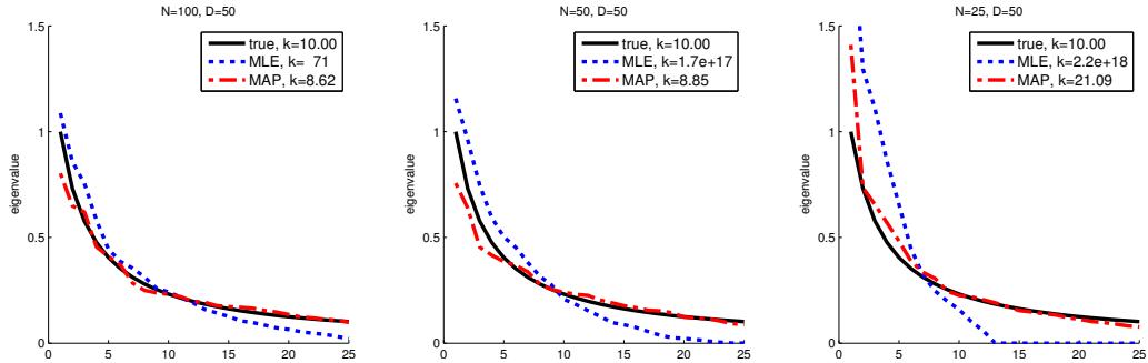
Figure 4.4: Estimating a covariance matrix in D = 50 dimensions using N ⇒ {100, 50, 25} samples. We plot the eigenvalues in descending order for the true covariance matrix (solid black), the MLE (dotted blue) and the MAP estimate (dashed red), using Equation (4.98) with ↼ = 0.9. We also list the condition number of each matrix in the legend. We see that the MLE is often poorly conditioned, but the MAP estimate is numerically well behaved. Adapted from Figure 1 of [SS05]. Generated by shrinkcov\_plots.ipynb.

frequentist estimate if we use squared loss. This is implemented in the sklearn function https://scikitlearn.org/stable/modules/generated/sklearn.covariance.LedoitWolf.html.

The benefits of this approach are illustrated in Figure 4.4. We consider fitting a 50-dimensional Gaussian to N = 100, N = 50 and N = 25 data points. We see that the MAP estimate is always well-conditioned, unlike the MLE (see Section 7.1.4.4 for a discussion of condition numbers). In particular, we see that the eigenvalue spectrum of the MAP estimate is much closer to that of the true matrix than the MLE’s spectrum. The eigenvectors, however, are una!ected.

4.5.3 Example: weight decay

In Figure 1.7, we saw how using polynomial regression with too high of a degree can result in overfitting. One solution is to reduce the degree of the polynomial. However, a more general solution is to penalize the magnitude of the weights (regression coe”cients). We can do this by using a zero-mean Gaussian prior, p(w). The resulting MAP estimate is given by

\[ \hat{w}\_{\text{map}} = \underset{\mathbf{w}}{\text{argmin}} \, \text{NLL}(\mathbf{w}) + \lambda ||\mathbf{w}||\_2^2 \tag{4.99} \]

where ||w||^{2 2 =} $^{D d}=1 w^{2 d}. (We write w rather than ω, since it only really make sense to penalize the magnitude of weight vectors, rather than other parameters, such as bias terms or noise variances.)

Equation (4.99) is called ω² regularization or weight decay. The larger the value of φ, the more the parameters are penalized for being “large” (deviating from the zero-mean prior), and thus the less flexible the model.

In the case of linear regression, this kind of penalization scheme is called ridge regression. For example, consider the polynomial regression example from Section 1.2.2.2, where the predictor has the form

\[f(x; w) = \sum\_{d=0}^{D} w\_d x^d = w^\top [1, x, x^2, \dots, x^D] \tag{4.100}\]

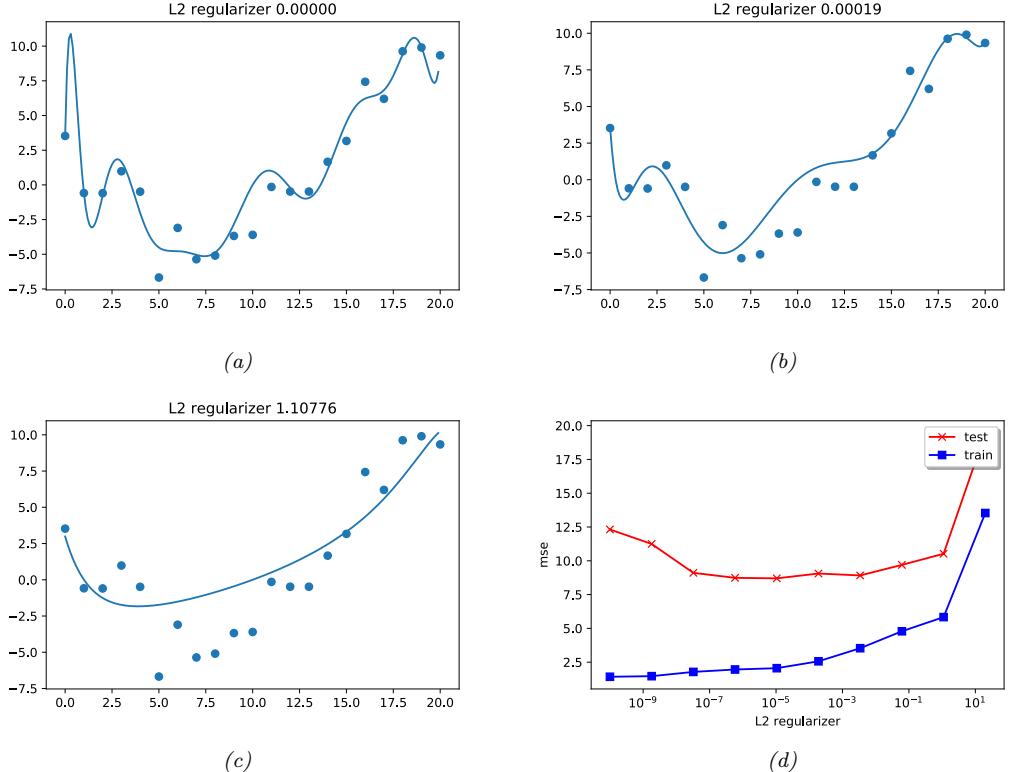
Figure 4.5: (a-c) Ridge regression applied to a degree 14 polynomial fit to 21 datapoints. (d) MSE vs strength of regularizer. The degree of regularization increases from left to right, so model complexity decreases from left to right. Generated by linreg\_poly\_ridge.ipynb.

Suppose we use a high degree polynomial, say D = 14, even though we have a small dataset with just N = 21 examples. MLE for the parameters will enable the model to fit the data very well, by carefully adjusting the weights, but the resulting function is very “wiggly”, thus resulting in overfitting. Figure 4.5 illustrates how increasing φ can reduce overfitting. For more details on ridge regression, see Section 11.3.

4.5.4 Picking the regularizer using a validation set

A key question when using regularization is how to choose the strength of the regularizer φ: a small value means we will focus on minimizing empirical risk, which may result in overfitting, whereas a large value means we will focus on staying close to the prior, which may result in underfitting.

In this section, we describe a simple but very widely used method for choosing φ. The basic idea is to partition the data into two disjoint sets, the training set Dtrain and a validation set Dvalid (also called a development set). (Often we use about 80% of the data for the training set, and

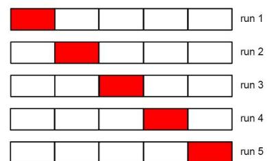
Figure 4.6: Schematic of 5-fold cross validation.

20% for the validation set.) We fit the model on Dtrain (for each setting of φ) and then evaluate its performance on Dvalid. We then pick the value of φ that results in the best validation performance. (This optimization method is a 1d example of grid search, discussed in Section 8.8.)

To explain the method in more detail, we need some notation. Let us define the regularized empirical risk on a dataset as follows:

\[R\_{\lambda}(\theta, \mathcal{D}) = \frac{1}{|\mathcal{D}|} \sum\_{(x, y) \in \mathcal{D}} \ell(y, f(x; \theta)) + \lambda C(\theta) \tag{4.101}\]

For each φ, we compute the parameter estimate

\[ \hat{\boldsymbol{\theta}}\_{\lambda}(\mathcal{D}\_{\text{train}}) = \underset{\boldsymbol{\theta}}{\text{argmin}} \, R\_{\lambda}(\boldsymbol{\theta}, \mathcal{D}\_{\text{train}}) \tag{4.102} \]

We then compute the validation risk:

\[R\_{\lambda}^{\text{val}} \stackrel{\Delta}{=} R\_0(\hat{\boldsymbol{\theta}}\_{\lambda}(\mathcal{D}\_{\text{train}}), \mathcal{D}\_{\text{valid}}) \tag{4.103}\]

This is an estimate of the population risk, which is the expected loss under the true distribution p↓(x, y). Finally we pick

\[\lambda^\* = \operatorname\*{argmin}\_{\lambda \in \mathcal{S}} R\_{\lambda}^{\text{val}} \tag{4.104}\]

(This requires fitting the model once for each value of φ in S, although in some cases, this can be done more e”ciently.)

After picking φ↓, we can refit the model to the entire dataset, D = Dtrain ∀ Dvalid, to get

\[\hat{\boldsymbol{\theta}}^{\*} = \operatorname\*{argmin}\_{\boldsymbol{\theta}} R\_{\lambda^\*} (\boldsymbol{\theta}, \mathcal{D}) \tag{4.105}\]

4.5.5 Cross-validation

The above technique in Section 4.5.4 can work very well. However, if the size of the training set is small, leaving aside 20% for a validation set can result in an unreliable estimate of the model parameters.

A simple but popular solution to this is to use cross validation (CV). The idea is as follows: we split the training data into K folds; then, for each fold k → {1,…,K}, we train on all the folds but the k’th, and test on the k’th, in a round-robin fashion, as sketched in Figure 4.6. Formally, we have

\[R\_{\lambda}^{\text{cv}} \triangleq \frac{1}{K} \sum\_{k=1}^{K} R\_0(\hat{\theta}\_{\lambda}(\mathcal{D}\_{-k}), \mathcal{D}\_k) \tag{4.106}\]

where D^k is the data in the k’th fold, and D→^k is all the other data. This is called the cross-validated risk. Figure 4.6 illustrates this procedure for K = 5. If we set K = N, we get a method known as leave-one-out cross-validation, since we always train on N ↑ 1 items and test on the remaining one.

We can use the CV estimate as an objective inside of an optimization routine to pick the optimal hyperparameter, ^{φˆ =} argmin↼ ^Rcv ↼ . Finally we combine all the available data (training and validation), and re-estimate the model parameters using ^{ωˆ =} argmin^{ω R}↼ˆ(ω, ^D). See Section 5.4.3 for more details.

4.5.5.1 The one standard error rule

CV gives an estimate of Rˆ↼, but does not give any measure of uncertainty. A standard frequentist measure of uncertainty of an estimate is the standard error of the mean, which is the mean of the sampling distribution of the estimate (see Section 4.7.1). We can compute this as follows. First let ^{Ln = ω}(yn, f(xn; ^ωˆ↼(D→n)) be the loss on the ⁿ’th example, where we use the parameters that were estimated using whichever training fold excludes n. (Note that Lⁿ depends on φ, but we drop this from the notation.) Next let µˆ = ¹ N $^{N n}=1 Lⁿ be the empirical mean and εˆ² = ¹ N $^{N n}=1(L^{n ↑ µ}ˆ)² be the empirical variance. Given this, we define our estimate to be µˆ, and the standard error of this estimate to be se(µˆ) = ⇐ε^{ˆ N} . Note that ε measures the intrinsic variability of Lⁿ across samples, whereas se(ˆµ) measures our uncertainty about the mean µˆ.

Suppose we apply CV to a set of models and compute the mean and se of their estimated risks. A common heuristic for picking a model from these noisy estimates is to pick the value which corresponds to the simplest model whose risk is no more than one standard error above the risk of the best model; this is called the one-standard error rule [HTF01, p216].

4.5.5.2 Example: ridge regression

As an example, consider picking the strength of the ω² regularizer for the ridge regression problem in Section 4.5.3. In Figure 4.7a, we plot the error vs log(φ) on the train set (blue) and test set (red curve). We see that the test error has a U-shaped curve, where it decreases as we increase the regularizer, and then increases as we start to underfit. In Figure 4.7b, we plot the 5-fold CV estimate of the test MSE vs log(φ). We see that the minimum CV error is close the optimal value for the test set (although it does underestimate the spike in the test error for large lambda, due to the small sample size.)

4.5.6 Early stopping

A very simple form of regularization, which is often very e!ective in practice (especially for complex models), is known as early stopping. This leverages the fact that optimization algorithms are

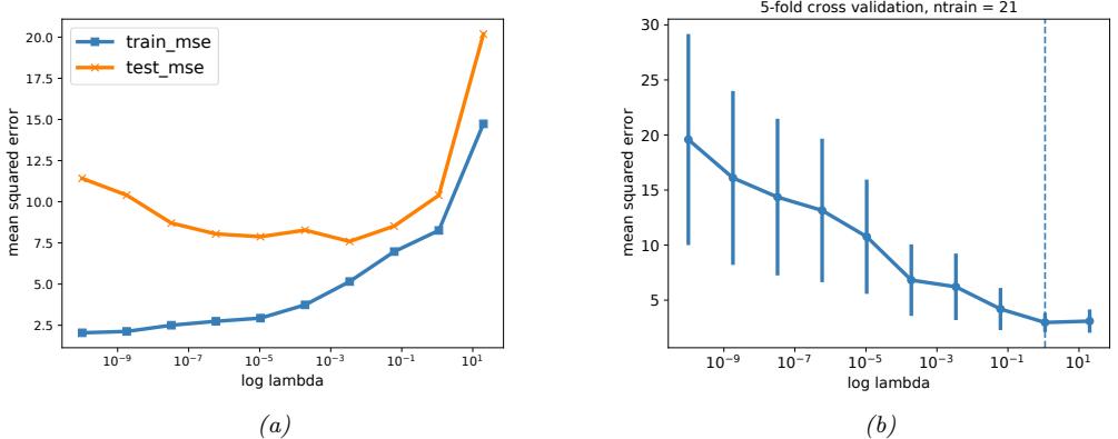
Figure 4.7: Ridge regression is applied to a degree 14 polynomial fit to 21 datapoints shown in Figure 4.5 for di!erent values of the regularizer ↼. The degree of regularization increases from left to right, so model complexity decreases from left to right. (a) MSE on train (blue) and test (red) vs log(↼). (b) 5-fold crossvalidation estimate of test MSE; error bars are standard error of the mean. Vertical line is the point chosen by the one standard error rule. Generated by polyfitRidgeCV.ipynb.

iterative, and so they take many steps to move away from the initial parameter estimates. If we detect signs of overfitting (by monitoring performance on the validation set), we can stop the optimization process, to prevent the model memorizing too much information about the training set. See Figure 4.8 for an illustration.

4.5.7 Using more data

As the amount of data increases, the chance of overfitting (for a model of fixed complexity) decreases (assuming the data contains suitably informative examples, and is not too redundant). This is illustrated in Figure 4.9. We show the MSE on the training and test sets for four di!erent models (polynomials of increasing degree) as a function of the training set size N. (A plot of error vs training set size is known as a learning curve.) The horizontal black line represents the Bayes error, which is the error of the optimal predictor (the true model) due to inherent noise. (In this example, the true model is a degree 2 polynomial, and the noise has a variance of ε² = 4; this is called the noise floor, since we cannot go below it.)

We notice several interesting things. First, the test error for degree 1 remains high, even as N increases, since the model is too simple to capture the truth; this is called underfitting. The test error for the other models decreases to the optimal level (the noise floor), but it decreases more rapidly for the simpler models, since they have fewer parameters to estimate. The gap between the test error and training error is larger for more complex models, but decreases as N grows.

Another interesting thing we can note is that the training error (blue line) initially increases with N, at least for the models that are su”ciently flexible. The reason for this is as follows: as the data set gets larger, we observe more distinct input-output pattern combinations, so the task of fitting the data becomes harder. However, eventually the training set will come to resemble the test set, and

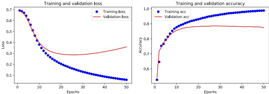
Figure 4.8: Performance of a text classifier (a neural network applied to a bag of word embeddings using average pooling) vs number of training epochs on the IMDB movie sentiment dataset. Blue = train, red = validation. (a) Cross entropy loss. Early stopping is triggered at about epoch 25. (b) Classification accuracy. Generated by imdb\_mlp\_bow\_tf.ipynb.

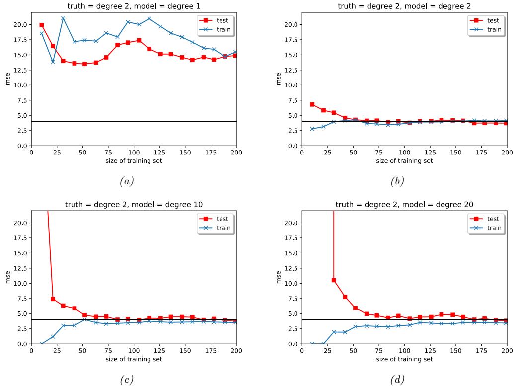
Figure 4.9: MSE on training and test sets vs size of training set, for data generated from a degree 2 polynomial with Gaussian noise of variance ϑ² = 4. We fit polynomial models of varying degree to this data. Generated by linreg\_poly\_vs\_n.ipynb.

the error rates will converge, and will reflect the optimal performance of that model.

4.6 Bayesian statistics *

So far, we have discussed several ways to estimate parameters from data. However, these approaches ignore any uncertainty in the estimates, which can be important for some applications, such as active learning, or avoiding overfitting, or just knowing how much to trust the estimate of some scientifically meaningful quantity. In statistics, modeling uncertainty about parameters using a probability distribution (as opposed to just computing a point estimate) is known as inference.

In this section, we use the posterior distribution to represent our uncertainty. This is the approach adopted in the field of Bayesian statistics. We give a brief introduction here, but more details can be found in the sequel to this book, [Mur23], as well as other good books, such as [Lam18; Kru15; McE20; Gel+14; MKL21; MFR20].

To compute the posterior, we start with a prior distribution p(ω), which reflects what we know before seeing the data. We then define a likelihood function p(D|ω), which reflects the data we expect to see for each setting of the parameters. We then use Bayes rule to condition the prior on the observed data to compute the posterior p(ω|D) as follows:

\[p(\boldsymbol{\theta}|\mathcal{D}) = \frac{p(\boldsymbol{\theta})p(\mathcal{D}|\boldsymbol{\theta})}{p(\mathcal{D})} = \frac{p(\boldsymbol{\theta})p(\mathcal{D}|\boldsymbol{\theta})}{\int p(\boldsymbol{\theta}')p(\mathcal{D}|\boldsymbol{\theta}')d\boldsymbol{\theta}'} \tag{4.107}\]

The denominator p(D) is called the marginal likelihood, since it is computed by marginalizing over (or integrating out) the unknown ω. This can be interpreted as the average probability of the data, where the average is wrt the prior. Note, however, that p(D) is a constant, independent of ω, so we will often ignore it when we just want to infer the relative probabilities of ω values.

Equation (4.107) is analogous to the use of Bayes rule for COVID-19 testing in Section 2.3.1. The di!erence is that the unknowns correspond to parameters of a statistical model, rather than the unknown disease state of a patient. In addition, we usually condition on a set of observations D, as opposed to a single observation (such as a single test outcome). In particular, for a supervised or conditional model, the observed data has the form D = {(xn, yn) : n =1: N}. For an unsupervised or unconditional model, the observed data has the form D = {(yn) : n =1: N}.

Once we have computed the posterior over the parameters, we can compute the posterior predictive distribution over outputs given inputs by marginalizing out the unknown parameters. In the supervised/ conditional case, this becomes

\[p(\mathbf{y}|\mathbf{x}, \mathcal{D}) = \int p(\mathbf{y}|\mathbf{x}, \boldsymbol{\theta}) p(\boldsymbol{\theta}|\mathcal{D}) d\boldsymbol{\theta} \tag{4.108}\]

This can be viewed as a form of Bayes model averaging (BMA), since we are making predictions using an infinite set of models (parameter values), each one weighted by how likely it is. The use of BMA reduces the chance of overfitting (Section 1.2.3), since we are not just using the single best model.

4.6.1 Conjugate priors

In this section, we consider a set of (prior, likelihood) pairs for which we can compute the posterior in closed form. In particular, we will use priors that are “conjugate” to the likelihood. We say that

a prior p(ω) → F is a conjugate prior for a likelihood function p(D|ω) if the posterior is in the same parameterized family as the prior, i.e., p(ω|D) → F. In other words, F is closed under Bayesian updating. If the family F corresponds to the exponential family (defined in Section 3.4), then the computations can be performed in closed form.

In the sections below, we give some common examples of this framework, which we will use later in the book. For simplicity, we focus on unconditional models (i.e., there are only outcomes or targets y, and no inputs or features x); we relax this assumption in Section 4.6.7.

4.6.2 The beta-binomial model

Suppose we toss a coin N times, and want to infer the probability of heads. Let yⁿ = 1 denote the event that the n’th trial was heads, yⁿ = 0 represent the event that the n’th trial was tails, and let D = {yⁿ : n =1: N} be all the data. We assume yⁿ ⇒ Ber(ϖ), where ϖ → [0, 1] is the rate parameter (probability of heads). In this section, we discuss how to compute p(ϖ|D).

4.6.2.1 Bernoulli likelihood

We assume the data are iid or independent and identically distributed. Thus the likelihood has the form

\[p(\mathcal{D}|\theta) = \prod\_{n=1}^{N} \theta^{y\_n} (1-\theta)^{1-y\_n} = \theta^{N\_1} (1-\theta)^{N\_0} \tag{4.109}\]

where we have defined N¹ = $^{N n}=1 ^I(yⁿ = 1) and ^{N0 =} $^{N n}=1 I(yⁿ = 0), representing the number of heads and tails. These counts are called the su!cient statistics of the data, since this is all we need to know about D to infer ϖ. The total count, N = N⁰ + N1, is called the sample size.

4.6.2.2 Binomial likelihood

Note that we can also consider a Binomial likelihood model, in which we perform N trials and observe the number of heads, y, rather than observing a sequence of coin tosses. Now the likelihood has the following form:

\[p(\mathcal{D}|\theta) = \text{Bin}(y|N, \theta) = \binom{N}{y} \theta^y (1 - \theta)^{N - y} \tag{4.110}\]

The scaling factor .^N y / is independent of ϖ, so we can ignore it. Thus this likelihood is proportional to the Bernoulli likelihood in Equation (4.109), so our inferences about ϖ will be the same for both models.

4.6.2.3 Prior

To simplify the computations, we will assume that the prior p(ω) → F is a conjugate prior for the likelihood function p(y|ω). This means that the posterior is in the same parameterized family as the prior, i.e., p(ω|D) → F.

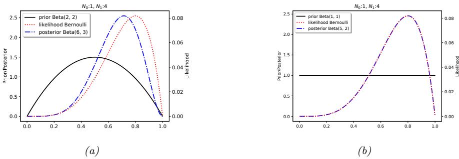
Figure 4.10: Updating a Beta prior with a Bernoulli likelihood with su”cient statistics N¹ = 4, N⁰ = 1. (a) Beta(2,2) prior. (b) Uniform Beta(1,1) prior. Generated by beta\_binom\_post\_plot.ipynb.

To ensure this property when using the Bernoulli (or Binomial) likelihood, we should use a prior of the following form:

\[p(\theta) \propto \theta^{\check{\theta}-1} (1-\theta)^{\check{\beta}-1} \propto \text{Beta}(\theta | \check{\alpha}, \check{\beta}) \tag{4.111}\]

We recognize this as the pdf of a beta distribution (see Section 2.7.4).

4.6.2.4 Posterior

If we multiply the Bernoulli likelihood in Equation (4.109) with the beta prior in Equation (2.136) we get a beta posterior:

\[p(\theta|\mathcal{D}) \propto \theta^{N\_1} (1-\theta)^{N\_0} \theta^{\mathbb{M}-1} (1-\theta)^{\overset{\mathcal{Y}}{\mathbb{X}}-1} \tag{4.112}\]

\[\propto \text{Beta}(\theta | \check{\alpha} + N\_1, \check{\beta} + N\_0) \tag{4.113}\]

\[\mathbf{u} = \text{Beta}(\boldsymbol{\theta} | \, \hat{\boldsymbol{\alpha}}, \hat{\boldsymbol{\beta}}) \tag{4.114}\]

where ↭ϱ↭↫^{ϱ +}N¹ and ↭ ¹↭↫ 1 +N⁰ are the parameters of the posterior. Since the posterior has the same functional form as the prior, we say that the beta distribution is a conjugate prior for the Bernoulli likelihood.

The parameters of the prior are called hyper-parameters. It is clear that (in this example) the hyper-parameters play a role analogous to the su”cient statistics; they are therefore often called pseudo counts. We see that we can compute the posterior by simply adding the observed counts (from the likelihood) to the pseudo counts (from the prior).

The strength of the prior is controlled by ↫ ^N=↫^{ϱ +} ↫ 1; this is called the equivalent sample size, since it plays a role analogous to the observed sample size, N = N⁰ + N1.

4.6.2.5 Example

For example, suppose we set ↫ϱ=↫ 1= 2. This is like saying we believe we have already seen two heads and two tails before we see the actual data; this is a very weak preference for the value of ϖ = 0.5.

The e!ect of using this prior is illustrated in Figure 4.10a. We see the posterior (blue line) is a “compromise” between the prior (red line) and the likelihood (black line).

If we set ↫ϱ=↫ 1= 1, the corresponding prior becomes the uniform distribution:

\[p(\theta) = \text{Beta}(\theta|1, 1) \propto \theta^0 (1 - \theta)^0 = \text{Unif}(\theta|0, 1) \tag{4.115}\]

The e!ect of using this prior is illustrated in Figure 4.10b. We see that the posterior has exactly the same shape as the likelihood, since the prior was “uninformative”.

4.6.2.6 Posterior mode (MAP estimate)

The most probable value of the parameter is given by the MAP estimate

\[\hat{\theta}\_{\text{map}} = \arg\max\_{\theta} p(\theta|\mathcal{D}) \tag{4.116}\]

\[\theta = \arg\max\_{\theta} \log p(\theta|\mathcal{D}) \tag{4.117}\]

\[\delta = \arg\max\_{\theta} \log p(\theta) + \log p(\mathcal{D}|\theta) \tag{4.118}\]

Using calculus, one can show that this is given by

\[\hat{\theta}\_{\text{map}} = \frac{\mathbb{X} + N\_1 - 1}{\mathbb{X} + N\_1 - 1 + \overline{\beta} + N\_0 - 1} \tag{4.119}\]

If we use a Beta(ϖ|2, 2) prior, this amounts to add-one smoothing:

\[\hat{\theta}\_{\text{map}} = \frac{N\_1 + 1}{N\_1 + 1 + N\_0 + 1} = \frac{N\_1 + 1}{N + 2} \tag{4.120}\]

If we use a uniform prior, p(ϖ) ∞ 1, the MAP estimate becomes the MLE, since log p(ϖ)=0:

\[\hat{\theta}\_{\text{mle}} = \arg\max\_{\theta} \log p(\mathcal{D}|\theta) \tag{4.121}\]

When we use a Beta prior, the uniform distribution is ↫ϱ=↫ 1= 1. In this case, the MAP estimate reduces to the MLE:

\[ \hat{\theta}\_{\text{mle}} = \frac{N\_1}{N\_1 + N\_0} = \frac{N\_1}{N} \tag{4.122} \]

If N¹ = 0, we will estimate that p(Y = 1) = 0.0, which says that we do not predict any future observations to be 1. This is a very extreme estimate, that is likely due to insu”cient data. We can solve this problem using a MAP estimate with a stronger prior, or using a fully Bayesian approach, in which we marginalize out ϖ instead of estimating it, as explained in Section 4.6.2.9.

4.6.2.7 Posterior mean

The posterior mode can be a poor summary of the posterior, since it corresponds to a single point. The posterior mean is a more robust estimate, since it integrates over the whole space.

If ^p(ϖ|D) = Beta(ϖ^| ↭ϱ, ↭ 1), then the posterior mean is given by

\[\overline{\theta} \triangleq \mathbb{E}\left[\theta | \mathcal{D}\right] = \frac{\widehat{\alpha}}{\widehat{\beta} + \widehat{\alpha}} = \frac{\widehat{\alpha}}{\widehat{N}} \tag{4.123}\]

where ↭ N=↭ 1 + ↭ϱ is the strength (equivalent sample size) of the posterior.

We will now show that the posterior mean is a convex combination of the prior mean, m =↫ϱ / ↫ N (where ↫ ^N↭↫^{ϱ +} ↫ 1 is the prior strength), and the MLE: ˆϖmle = ^N1 N :

\[\mathbb{E}\left[\theta|\mathcal{D}\right] = \frac{\check{\alpha} + N\_1}{\check{\alpha} + N\_1 + \check{\beta} + N\_0} = \frac{\check{N}\,m + N\_1}{N + \check{N}} = \frac{\check{N}}{N + \check{N}}\,m + \frac{N}{N + \check{N}}\frac{N\_1}{N} = \lambda m + (1 - \lambda)\hat{\theta}\_{\text{mle}} \tag{4.124}\]

where ^{φ =} ↫ N↭ ^N is the ratio of the prior to posterior equivalent sample size. So the weaker the prior, the smaller is φ, and hence the closer the posterior mean is to the MLE.

4.6.2.8 Posterior variance

To capture some notion of uncertainty in our estimate, a common approach is to compute the standard error of our estimate, which is just the posterior standard deviation:

\[\text{se}(\theta) = \sqrt{\mathbb{V}\left[\theta|\mathcal{D}\right]} \tag{4.125}\]

In the case of the Bernoulli model, we showed that the posterior is a beta distribution. The variance of the beta posterior is given by

\[\mathbb{V}\left[\theta|\mathcal{D}\right] = \frac{\widehat{\alpha}\widehat{\beta}}{(\widehat{\alpha}+\widehat{\beta})^2(\widehat{\alpha}+\widehat{\beta}+1)} = \mathbb{E}\left[\theta|\mathcal{D}\right]^2 \frac{\widehat{\beta}}{\widehat{\alpha}\left(1+\widehat{\alpha}+\widehat{\beta}\right)}\tag{4.126}\]

where ↭ϱ=↫^{ϱ +}N¹ and ↭ 1=↫ ^{1 +}N0. If ^N ⇐↫^{ϱ +} ↫ 1, this simplifies to

\[\mathbb{V}\left[\theta|\mathcal{D}\right] \approx \frac{N\_1 N\_0}{N^3} = \frac{\hat{\theta}(1-\hat{\theta})}{N} \tag{4.127}\]

where ˆϖ is the MLE. Hence the standard error is given by

\[ \sigma = \sqrt{\mathbb{V}\left[\theta|\mathcal{D}\right]} \approx \sqrt{\frac{\hat{\theta}(1-\hat{\theta})}{N}} \tag{4.128} \]

We see that the uncertainty goes down at a rate of 1/ ≃ N. We also see that the uncertainty (variance) is maximized when ˆϖ = 0.5, and is minimized when ˆϖ is close to 0 or 1. This makes sense, since it is easier to be sure that a coin is biased than to be sure that it is fair.

4.6.2.9 Posterior predictive

Suppose we want to predict future observations. A very common approach is to first compute an estimate of the parameters based on training data, ^ωˆ(D), and then to plug that parameter back into the model and use ^p(y|ωˆ) to predict the future; this is called a plug-in approximation. However, this can result in overfitting. As an extreme example, suppose we have seen N = 3 heads in a row. The MLE is ˆϖ = 3/3=1. However, if we use this estimate, we would predict that tails are impossible.

One solution to this is to compute a MAP estimate, and plug that in, as we discussed in Section 4.5.1. Here we discuss a fully Bayesian solution, in which we marginalize out ϖ.

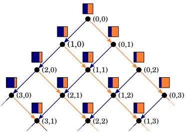
Figure 4.11: Illustration of sequential Bayesian updating for the beta-Bernoulli model. Each colored box represents the predicted distribution p(xt|ht), where h^t = (N1,t, N0,t) is the su”cient statistic derived from history of observations up until time t, namely the total number of heads and tails. The probability of heads (blue bar) is given by p(x^t = 1|ht)=(Nt,¹ + 1)/(t + 2), assuming we start with a uniform Beta(ε|1, 1) prior. From Figure 3 of [Ort+19]. Used with kind permission of Pedro Ortega.

Bernoulli model

For the Bernoulli model, the resulting posterior predictive distribution has the form

\[\begin{split} p(y=1|\mathcal{D}) &= \int\_0^1 p(y=1|\theta)p(\theta|\mathcal{D})d\theta \\ &= \int\_0^1 \theta \operatorname{Beta}(\theta|\,\widehat{\alpha}, \widehat{\beta})d\theta = \mathbb{E}\left[\theta|\mathcal{D}\right] = \frac{\widehat{\alpha}}{\widehat{\alpha} + \widehat{\beta}} \end{split} \tag{4.130}\]

In Section 4.5.1, we had to use the Beta(2,2) prior to recover add-one smoothing, which is a rather unnatural prior. In the Bayesian approach, we can get the same e!ect using a uniform prior, p(ϖ) = Beta(ϖ|1, 1), since the predictive distribution becomes

\[p(y=1|\mathcal{D}) = \frac{N\_1 + 1}{N\_1 + N\_0 + 2} \tag{4.131}\]

This is known as Laplace’s rule of succession. See Figure 4.11 for an illustration of this in the sequential setting.

Binomial model

Now suppose we were interested in predicting the number of heads in M > 1 future coin tossing trials, i.e., we are using the binomial model instead of the Bernoulli model. The posterior over ϖ is the same as before, but the posterior predictive distribution is di!erent:

\[p(y|\mathcal{D},M) = \int\_0^1 \text{Bin}(y|M,\theta)\text{Beta}(\theta|\stackrel{\frown}{\alpha},\widehat{\beta})d\theta\tag{4.132}\]

\[= \binom{M}{y} \frac{1}{B(\widehat{\alpha}, \widehat{\beta})} \int\_0^1 \theta^y (1 - \theta)^{M - y} \theta^{\widehat{\alpha} - 1} (1 - \theta)^{\widehat{\beta} - 1} d\theta \tag{4.133}\]

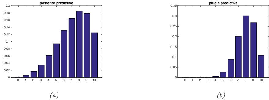
Figure 4.12: (a) Posterior predictive distributions for 10 future trials after seeing N¹ = 4 heads and N⁰ = 1 tails. (b) Plug-in approximation based on the same data. In both cases, we use a uniform prior. Generated by beta\_binom\_post\_pred\_plot.ipynb.

We recognize the integral as the normalization constant for a Beta( ↭^{ϱ +}y,M ^{↑ y+} ↭ 1) distribution. Hence

\[\int\_0^1 \theta^{y+\widehat{\alpha}-1} (1-\theta)^{M-y+\widehat{\beta}-1} d\theta = B(y+\widehat{\alpha}, M-y+\widehat{\beta})\tag{4.134}\]

Thus we find that the posterior predictive is given by the following, known as the (compound) beta-binomial distribution:

\[Bb(x|M,\hat{\alpha},\hat{\beta}) \triangleq \binom{M}{x} \frac{B(x+\hat{\alpha}, M-x+\hat{\beta})}{B(\hat{\alpha},\hat{\beta})} \tag{4.135}\]

In Figure 4.12(a), we plot the posterior predictive density for M = 10 after seeing N¹ = 4 heads and N⁰ = 1 tails, when using a uniform Beta(1,1) prior. In Figure 4.12(b), we plot the plug-in approximation, given by

\[p(\theta|\mathcal{D}) \approx \delta(\theta - \hat{\theta}) \tag{4.136}\]

\[p(y|\mathcal{D},M) = \int\_0^1 \text{Bin}(y|M,\theta)p(\theta|\mathcal{D})d\theta = \text{Bin}(y|M,\hat{\theta})\tag{4.137}\]

where ˆϖ is the MAP estimate. Looking at Figure 4.12, we see that the Bayesian prediction has longer tails, spreading its probability mass more widely, and is therefore less prone to overfitting and black-swan type paradoxes. (Note that we use a uniform prior in both cases, so the di!erence is not arising due to the use of a prior; rather, it is due to the fact that the Bayesian approach integrates out the unknown parameters when making its predictions.)

4.6.2.10 Marginal likelihood

The marginal likelihood or evidence for a model M is defined as

\[p(\mathcal{D}|\mathcal{M}) = \int p(\boldsymbol{\theta}|\mathcal{M}) p(\mathcal{D}|\boldsymbol{\theta}, \mathcal{M}) d\boldsymbol{\theta} \tag{4.138}\]

When performing inference for the parameters of a specific model, we can ignore this term, since it is constant wrt ω. However, this quantity plays a vital role when choosing between di!erent models, as we discuss in Section 5.2.2. It is also useful for estimating the hyperparameters from data (an approach known as empirical Bayes), as we discuss in Section 4.6.5.3.

In general, computing the marginal likelihood can be hard. However, in the case of the beta-Bernoulli model, the marginal likelihood is proportional to the ratio of the posterior normalizer to the prior normalizer. To see this, recall that the posterior for the beta-binomial models is given by p(ϖ|D) = Beta(ϖ|a↗ , b↗ ), where a↗ = a + N¹ and b↗ = b + N0. We know the normalization constant of the posterior is B(a↗ , b↗ ). Hence

\[p(\theta|\mathcal{D}) = \frac{p(\mathcal{D}|\theta)p(\theta)}{p(\mathcal{D})} \tag{4.139}\]

\[\hat{\theta}\_{1} = \frac{1}{p(\mathcal{D})} \left[ \frac{1}{B(a, b)} \theta^{a-1} (1 - \theta)^{b-1} \right] \left[ \binom{N}{N\_1} \theta^{N\_1} (1 - \theta)^{N\_0} \right] \tag{4.140}\]

\[\hat{\theta} = \binom{N}{N\_1} \frac{1}{p(\mathcal{D})} \frac{1}{B(a, b)} \left[ \theta^{a + N\_1 - 1} (1 - \theta)^{b + N\_0 - 1} \right] \tag{4.141}\]

So

\[\frac{1}{B(a+N\_1, b+N\_0)} = \binom{N}{N\_1} \frac{1}{p(\mathcal{D})} \frac{1}{B(a,b)}\tag{4.142}\]

\[p(\mathcal{D}) = \binom{N}{N\_1} \frac{B(a+N\_1, b+N\_0)}{B(a,b)}\tag{4.143}\]

The marginal likelihood for the beta-Bernoulli model is the same as above, except it is missing the ’ N N¹ ( term.

4.6.2.11 Mixtures of conjugate priors

The beta distribution is a conjugate prior for the binomial likelihood, which enables us to easily compute the posterior in closed form, as we have seen. However, this prior is rather restrictive. For example, suppose we want to predict the outcome of a coin toss at a casino, and we believe that the coin may be fair, but may equally likely be biased towards heads. This prior cannot be represented by a beta distribution. Fortunately, it can be represented as a mixture of beta distributions. For example, we might use

\[p(\theta) = 0.5 \text{Beta}(\theta | 20, 20) + 0.5 \text{Beta}(\theta | 30, 10) \tag{4.144}\]

If ϖ comes from the first distribution, the coin is fair, but if it comes from the second, it is biased towards heads.

We can represent a mixture by introducing a latent indicator variable h, where h = k means that ϖ comes from mixture component k. The prior has the form

\[p(\theta) = \sum\_{k} p(h=k)p(\theta|h=k) \tag{4.145}\]

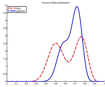
Figure 4.13: A mixture of two Beta distributions. Generated by mixbetademo.ipynb.

where each p(ϖ|h = k) is conjugate, and p(h = k) are called the (prior) mixing weights. One can show (Exercise 4.6) that the posterior can also be written as a mixture of conjugate distributions as follows:

\[p(\theta|\mathcal{D}) = \sum\_{k} p(h=k|\mathcal{D})p(\theta|\mathcal{D}, h=k) \tag{4.146}\]

where p(h = k|D) are the posterior mixing weights given by

\[p(h=k|\mathcal{D}) = \frac{p(h=k)p(\mathcal{D}|h=k)}{\sum\_{k'} p(h=k')p(\mathcal{D}|h=k')}\tag{4.147}\]

Here the quantity p(D|h = k) is the marginal likelihood for mixture component k (see Section 4.6.2.10).

Returning to our example above, if we have the prior in Equation (4.144), and we observe N¹ = 20 heads and N⁰ = 10 tails, then, using Equation (4.143), the posterior becomes

\[p(\theta|\mathcal{D}) = 0.346 \operatorname{Beta}(\theta|40, 30) + 0.654 \operatorname{Beta}(\theta|50, 20) \tag{4.148}\]

See Figure 4.13 for an illustration.

We can compute the posterior probability that the coin is biased towards heads as follows:

\[\Pr(\theta > 0.5 | \mathcal{D}) = \sum\_{k} \Pr(\theta > 0.5 | \mathcal{D}, h = k) p(h = k | \mathcal{D}) = 0.9604 \tag{4.149}\]

If we just used a single Beta(20,20) prior, we would get a slightly smaller value of Pr(ϖ > 0.5|D) = 0.8858. So if we were “suspicious” initially that the casino might be using a biased coin, our fears would be confirmed more quickly than if we had to be convinced starting with an open mind.

4.6.3 The Dirichlet-multinomial model

In this section, we generalize the results from Section 4.6.2 from binary variables (e.g., coins) to K-ary variables (e.g., dice).

4.6.3.1 Likelihood

Let Y ⇒ Cat(ω) be a discrete random variable drawn from a categorical distribution. The likelihood has the form

\[p(\mathcal{D}|\boldsymbol{\theta}) = \prod\_{n=1}^{N} \text{Cat}(y\_n|\boldsymbol{\theta}) = \prod\_{n=1}^{N} \prod\_{c=1}^{C} \theta\_c^{\mathbb{I}(y\_n=c)} = \prod\_{c=1}^{C} \theta\_c^{N\_c} \tag{4.150}\] \(\text{where } N\_c = \sum\_n \mathbb{I}(y\_n = c).\)

where N^c = $ ⁿ I(yⁿ = c).

4.6.3.2 Prior

The conjugate prior for a categorical distribution is the Dirichlet distribution, which is a multivariate generalization of the beta distribution. This has support over the probability simplex, defined by

\[S\_K = \{ \theta : 0 \le \theta\_k \le 1, \sum\_{k=1}^K \theta\_k = 1 \}\tag{4.151}\]

The pdf of the Dirichlet is defined as follows:

\[\text{Dir}(\theta|\,\check{\alpha}) \triangleq \frac{1}{B(\check{\alpha})} \prod\_{k=1}^{K} \theta\_k^{\check{\alpha}\_k - 1} \mathbb{1}(\theta \in S\_K) \tag{4.152}\]

where B(↫φ) is the multivariate beta function,

\[B(\check{\alpha}) \stackrel{\Delta}{=} \frac{\prod\_{k=1}^{K} \Gamma(\check{\alpha}\_{k})}{\Gamma(\sum\_{k=1}^{K} \check{\alpha}\_{k})} \tag{4.153}\]

Figure 4.14 shows some plots of the Dirichlet when K = 3. We see that ↫ϱ0= $ k ↫ϱ^k controls the strength of the distribution (how peaked it is), and the ↫ϱ^k control where the peak occurs. For example, Dir(1, 1, 1) is a uniform distribution, Dir(2, 2, 2) is a broad distribution centered at (1/3, 1/3, 1/3), and Dir(20, 20, 20) is a narrow distribution centered at (1/3, 1/3, 1/3). Dir(3, 3, 20) is an asymmetric distribution that puts more density in one of the corners. If ↫ϱk< 1 for all k, we get “spikes” at the corners of the simplex. Samples from the distribution when ↫ϱk< 1 will be sparse, as shown in Figure 4.15.

4.6.3.3 Posterior

We can combine the multinomial likelihood and Dirichlet prior to compute the posterior, as follows:

\[p(\boldsymbol{\theta}|\mathcal{D}) \propto p(\mathcal{D}|\boldsymbol{\theta}) \text{Dir}(\boldsymbol{\theta}|\operatorname{\check{\alpha}}) \tag{4.154}\]

\[= \left[\prod\_{k} \theta\_{k}^{N\_{k}}\right] \left[\prod\_{k} \theta\_{k}^{\mathbb{X}\_{k}-1}\right] \tag{4.155}\]

\[\mathbf{h} = \text{Dir}(\boldsymbol{\theta}|\,\mathbb{X}\_1 + N\_1, \dots, \mathbb{X}\_K + N\_K) \tag{4.156}\]

\[=\text{Dir}(\theta|\,\hat{\alpha})\tag{4.157}\]

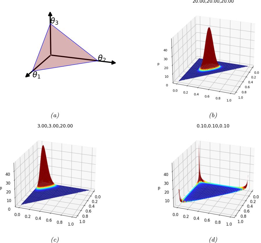
Figure 4.14: (a) The Dirichlet distribution when K = 3 defines a distribution over the simplex, which can be represented by the triangular surface. Points on this surface satisfy ⁰ ↗ ^εk ↗ ¹ and !^{3 k}=1 ε^k = 1. Generated by dirichlet\_3d\_triangle\_plot.ipynb. (b) Plot of the Dirichlet density for ↫ ε= (20, 20, 20). (c) Plot of the Dirichlet density for ↫ ε= (3, 3, 20). (d) Plot of the Dirichlet density for ↫ ε= (0.1, 0.1, 0.1). Generated by dirichlet\_3d\_spiky\_plot.ipynb.

where ↭ϱk=↫ϱ^k +N^k are the parameters of the posterior. So we see that the posterior can be computed by adding the empirical counts to the prior counts.

The posterior mean is given by

\[\overline{\theta}\_{k} = \frac{\widehat{\alpha}\_{k}}{\sum\_{k'=1}^{K} \widehat{\alpha}\_{k'}} \tag{4.158}\]

The posterior mode, which corresponds to the MAP estimate, is given by

\[\hat{\theta}\_k = \frac{\hat{\alpha}\_k - 1}{\sum\_{k'=1}^K (\hat{\alpha}\_{k'} - 1)}\tag{4.159}\]

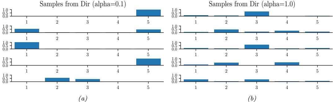
Figure 4.15: Samples from a 5-dimensional symmetric Dirichlet distribution for di!erent parameter values. (a) ↫ ε= (0.1,…, 0.1). This results in very sparse distributions, with many 0s. (b) ↫ ε= (1,…, 1). This results in more uniform (and dense) distributions. Generated by dirichlet\_samples\_plot.ipynb.

If we use ↫ϱk= 1, corresponding to a uniform prior, the MAP becomes the MLE:

\[ \hat{\theta}\_k = N\_k / N \tag{4.160} \]

(See Section 4.2.4 for a more direct derivation of this result.)

4.6.3.4 Posterior predictive

The posterior predictive distribution is given by

\[p(y=k|\mathcal{D}) = \int p(y=k|\theta)p(\theta|\mathcal{D})d\theta\tag{4.161}\]

\[=\int \theta\_k p(\theta\_k | \mathcal{D}) d\theta\_k = \mathbb{E}\left[\theta\_k | \mathcal{D}\right] = \frac{\widehat{\alpha}\_k}{\sum\_{k'} \widehat{\alpha}\_{k'}}\tag{4.162}\]

In other words, the posterior predictive distribution is given by

\[p(y|\mathcal{D}) = \text{Cat}(y|\overline{\theta})\tag{4.163}\]

where ω ↭ E [ω|D] are the posterior mean parameters. If instead we plug-in the MAP estimate, we will su!er from the zero-count problem. The only way to get the same e!ect as add-one smoothing is to use a MAP estimate with ↫ϱc= 2.

Equation (4.162) gives the probability of a single future event, conditioned on past observations y = (y1,…,y^N ). In some cases, we want to know the probability of observing a batch of future data, say y˜ = (˜y1,…, y˜M). We can compute this as follows:

\[p(\ddot{y}|y) = \frac{p(\ddot{y}, y)}{p(y)}\tag{4.164}\]

The denominator is the marginal likelihood of the training data, and the numerator is the marginal likelihood of the training and future test data. We discuss how to compute such marginal likelihoods in Section 4.6.3.5.

4.6.3.5 Marginal likelihood

By the same reasoning as in Section 4.6.2.10, one can show that the marginal likelihood for the Dirichlet-categorical model is given by

\[p(\mathcal{D}) = \frac{B(\mathbf{N} + \alpha)}{B(\alpha)}\tag{4.165}\]

where

\[B(\alpha) = \frac{\prod\_{k=1}^{K} \Gamma(\alpha\_k)}{\Gamma(\sum\_k \alpha\_k)} \tag{4.166}\]

Hence we can rewrite the above result in the following form, which is what is usually presented in the literature:

\[p(\mathcal{D}) = \frac{\Gamma(\sum\_{k} \alpha\_{k})}{\Gamma(N + \sum\_{k} \alpha\_{k})} \prod\_{k} \frac{\Gamma(N\_{k} + \alpha\_{k})}{\Gamma(\alpha\_{k})} \tag{4.167}\]

4.6.4 The Gaussian-Gaussian model

In this section, we derive the posterior for the parameters of a Gaussian distribution. For simplicity, we assume the variance is known. (The general case is discussed in the sequel to this book, [Mur23], as well as other standard references on Bayesian statistics.)

4.6.4.1 Univariate case

If ε² is a known constant, the likelihood for µ has the form

\[p(\mathcal{D}|\mu) \propto \exp\left(-\frac{1}{2\sigma^2} \sum\_{n=1}^{N} (y\_n - \mu)^2\right) \tag{4.168}\]

One can show that the conjugate prior is another Gaussian, N (µ| m ↫ , ↫τ ²). Applying Bayes’ rule for Gaussians, as in Section 4.6.4.1, we find that the corresponding posterior is given by

\[p(\boldsymbol{\mu}|\mathcal{D}, \sigma^2) = \mathcal{N}(\boldsymbol{\mu}|\mathcal{D}, \hat{\tau}^2) \tag{4.169}\]

\[\hat{\tau}^2 = \frac{1}{\frac{N}{\sigma^2} + \frac{1}{\tilde{\tau}^2}} = \frac{\sigma^2 \,\hat{\tau}^2}{N \,\hat{\tau}^2 + \sigma^2} \tag{4.170}\]

\[ \hat{m} = \hat{\tau}^2 \left( \frac{\dot{m}}{\dot{\tau}^2} + \frac{N\overline{y}}{\sigma^2} \right) = \frac{\sigma^2}{N \ \dot{\tau}^2 + \sigma^2} \ \not{m} + \frac{N \ \not{\tau}^2}{N \ \dot{\tau}^2 + \sigma^2} \overline{y} \tag{4.171} \]

where y ↭ ¹ N $^{N n}=1 yⁿ is the empirical mean.

This result is easier to understand if we work in terms of the precision parameters, which are just inverse variances. Specifically, let 2 = 1/ε² be the observation precision, and ↫ φ= 1/ ↫τ ² be the

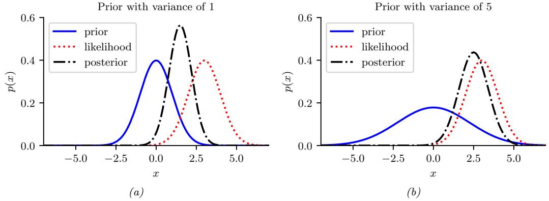
Figure 4.16: Inferring the mean of a univariate Gaussian with known ϑ² given observation y = 3. (a) Using strong prior, p(µ) = N (µ|0, 1). (b) Using weak prior, p(µ) = N (µ|0, 5). Generated by gauss\_infer\_1d.ipynb.

precision of the prior. We can then rewrite the posterior as follows:

\[p(\mu|\mathcal{D}, \kappa) = \mathcal{N}(\mu|\hat{m}, \hat{\lambda}^{-1})\tag{4.172}\]

\[ \widehat{\lambda} = \check{\lambda} + N\kappa \tag{4.173} \]

\[ \hbar \hbar = \frac{N\kappa \overline{y} + \stackrel{\leftrightarrow}{\lambda} \hbar \hbar}{\widehat{\lambda}} = \frac{N\kappa}{N\kappa + \stackrel{\leftrightarrow}{\lambda}} \overline{y} + \frac{\stackrel{\leftrightarrow}{\lambda}}{N\kappa + \stackrel{\leftrightarrow}{\lambda}} \, \hbar \, \tag{4.174} \]

These equations are quite intuitive: the posterior precision ↭ φ is the prior precision ↫ φ plus N units of measurement precision 2. Also, the posterior mean m ↭ is a convex combination of the empirical mean y and the prior mean m ↫ . This makes it clear that the posterior mean is a compromise between the empirical mean and the prior. If the prior is weak relative to the signal strength (↫ φ is small relative to 2), we put more weight on the empirical mean. If the prior is strong relative to the signal strength ( ↫ φ is large relative to 2), we put more weight on the prior. This is illustrated in Figure 4.16. Note also that the posterior mean is written in terms of N2y, so having N measurements each of precision 2 is like having one measurement with value y and precision N2.

Posterior after seeing N = 1 examples

To gain further insight into these equations, consider the posterior after seeing a single data point y (so N = 1). Then the posterior mean can be written in the following equivalent ways:

\[ \hat{\boldsymbol{m}} = \underset{\widetilde{\lambda}}{\overset{\textstyle \mathcal{K}}{\boldsymbol{\lambda}}} \overset{\textstyle \mathcal{K}}{\overset{\textstyle \mathcal{K}}{\boldsymbol{m}}} + \underset{\widetilde{\lambda}}{\overset{\textstyle \mathcal{K}}{\boldsymbol{\lambda}}} \tag{4.175} \]

\[ \dot{\lambda} = \dot{\mathcal{W}} + \frac{\kappa}{\overline{\lambda}} (y - \dot{\mathcal{W}}) \tag{4.176} \]

\[y = y - \frac{\check{\lambda}}{\check{\lambda}}(y - \mathcal{m})\tag{4.177}\]

The first equation is a convex combination of the prior mean and the data. The second equation is the prior mean adjusted towards the data y. The third equation is the data adjusted towards

the prior mean; this is called a shrinkage estimate. This is easier to see if we define the weight w = ↭ ↼/ ↫ ↼, which is the ratio of the prior to posterior precision. Then we have

\[ \hat{m} = y - w(y - \nw) = (1 - w)y + w \nmid\tag{4.178} \]

Note that, for a Gaussian, the posterior mean and posterior mode are the same. Thus we can use the above equations to perform MAP estimation. See Exercise 4.2 for a simple example.

Posterior variance

In addition to the posterior mean or mode of µ, we might be interested in the posterior variance, which gives us a measure of confidence in our estimate. The square root of this is called the standard error of the mean:

\[\text{se}(\mu) \triangleq \sqrt{\mathbb{V}[\mu|\mathcal{D}]} \tag{4.179}\]

Suppose we use an uninformative prior for µ by setting ↫ φ= 0 (see Section 4.6.5.1). In this case, the posterior mean is equal to the MLE, m ↭ = y. Suppose, in addition, that we approximate ε² by the sample variance

\[s^2 \triangleq \frac{1}{N} \sum\_{n=1}^{N} (y\_n - \overline{y})^2 \tag{4.180}\]

Hence ↭ φ= N2ˆ = N/s², so the SEM becomes

\[\text{se}(\mu) = \sqrt{\mathbb{V}\left[\mu | \mathcal{D}\right]} = \frac{1}{\sqrt{\lambda}} = \frac{s}{\sqrt{N}}\tag{4.181}\]

Thus we see that the uncertainty in µ is reduced at a rate of 1/ ≃ N.

In addition, we can use the fact that 95% of a Gaussian distribution is contained within 2 standard deviations of the mean to approximate the 95% credible interval for µ using

\[I\_{.95}(\mu|\mathcal{D}) = \overline{y} \pm 2\frac{s}{\sqrt{N}}\tag{4.182}\]

4.6.4.2 Multivariate case

For D-dimensional data, the likelihood has the following form (where we drop terms that are independent of µ):

\[p(\mathcal{D}|\boldsymbol{\mu}) = \prod\_{n=1}^{N} \mathcal{N}(y\_n|\boldsymbol{\mu}, \boldsymbol{\Sigma}) \tag{4.183}\]

\[= \left(\frac{1}{(2\pi)^{D/2}|\boldsymbol{\Sigma}|^{\frac{1}{2}}}\right)^{N} \exp\left[-\frac{1}{2}\sum\_{n=1}^{N}(y\_n - \mu)^{\mathsf{T}}\boldsymbol{\Sigma}^{-1}(y\_n - \mu)\right] \tag{4.184}\]

\[\varepsilon \propto \mathcal{N}(\overline{\mathfrak{y}}|\mu, \frac{1}{N}\Sigma) \tag{4.185}\]

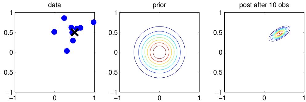
Figure 4.17: Illustration of Bayesian inference for the mean of a 2d Gaussian. (a) The data is generated from ^yn ↘ ^N (µ, !), where ^µ = [0.5, ⁰.5]^T and ! = 0.1[2, 1; 1, 1]). (b) The prior is ^p(µ) = ^N (µ|0, ⁰.1I2). (c) We show the posterior after 10 data points have been observed. Generated by gauss\_infer\_2d.ipynb.

where y = ¹ N $^{N n}=1 yn. (The proof of the last equation is given right after Equation (3.65).) Thus we replace the set of observations with their mean, and scale down the covariance by a factor of N.

For simplicity, we will use a conjugate prior, which in this case is a Gaussian, namely

\[p(\mu) = \mathcal{N}(\mu \mid \check{m}, \check{\mathbf{V}}) \tag{4.186}\]

We can derive a Gaussian posterior for µ based on the results in Section 3.3.1. We get

\[p(\boldsymbol{\mu}|\mathcal{D}, \boldsymbol{\Sigma}) = \mathcal{N}(\boldsymbol{\mu}|\,\hat{\boldsymbol{m}}, \hat{\mathbf{V}}) \tag{4.187}\]

\[ \hat{\mathbf{V}}^{-1} = \check{\mathbf{V}}^{-1} + N\boldsymbol{\Sigma}^{-1} \tag{4.188} \]

\[ \hat{m} = \hat{\mathbf{V}} \left( \boldsymbol{\Sigma}^{-1} (N \overline{\boldsymbol{y}}) + \check{\mathbf{V}}^{-1} \check{\mathbf{m}} \right) \tag{4.189} \]

Figure 4.17 gives a 2d example of these results.

4.6.5 Beyond conjugate priors

We have seen various examples of conjugate priors, all of which have come from the exponential family (see Section 3.4). These priors have the advantage of being easy to interpret (in terms of su”cient statistics from a virtual prior dataset), and easy to compute with. However, for most models, there is no prior in the exponential family that is conjugate to the likelihood. Furthermore, even where there is a conjugate prior, the assumption of conjugacy may be too limiting. Therefore in the sections below, we briefly discuss various other kinds of priors.

4.6.5.1 Noninformative priors

When we have little or no domain specific knowledge, it is desirable to use an uninformative, noninformative or objective priors, to “let the data speak for itself”. For example, if we want to infer a real valued quantity, such as a location parameter µ → R, we can use a flat prior p(µ) ∞ 1. This can be viewed as an “infinitely wide” Gaussian.

Unfortunately, there is no unique way to define uninformative priors, and they all encode some kind of knowledge. It is therefore better to use the term di”use prior, minimally informative prior or default prior. See the sequel to this book, [Mur23], for more details.

4.6.5.2 Hierarchical priors

Bayesian models require specifying a prior p(ω) for the parameters. The parameters of the prior are called hyperparameters, and will be denoted by ↼. If these are unknown, we can put a prior on them; this defines a hierarchical Bayesian model, or multi-level model, which can visualize like this: ↼ ↔︎ ω ↔︎ D. We assume the prior on the hyper-parameters is fixed (e.g., we may use some kind of minimally informative prior), so the joint distribution has the form

\[p(\xi, \theta, \mathcal{D}) = p(\xi)p(\theta|\xi)p(\mathcal{D}|\theta) \tag{4.190}\]

The hope is that we can learn the hyperparameters by treating the parameters themselves as datapoints. This is useful when we have multiple related parameters that need to be estimated (e.g., from di!erent subpopulations, or muliple tasks); this provides a learning signal to the top level of the model. See the sequel to this book, [Mur23], for details.

4.6.5.3 Empirical priors

In Section 4.6.5.2, we discussed hierarchical Bayes as a way to infer parameters from data. Unfortunately, posterior inference in such models can be computationally challenging. In this section, we discuss a computationally convenient approximation, in which we first compute a point estimate of the hyperparameters, ˆ ↼, and then compute the conditional posterior, ^p(ω|^ˆ ↼, D), rather than the joint posterior, p(ω, ↼|D).

To estimate the hyper-parameters, we can maximize the marginal likelihood:

\[\hat{\xi}\_{\text{mml}}(\mathcal{D}) = \underset{\mathfrak{E}}{\text{argmax}} \, p(\mathcal{D}|\boldsymbol{\xi}) = \underset{\mathfrak{E}}{\text{argmax}} \int p(\mathcal{D}|\boldsymbol{\theta}) p(\boldsymbol{\theta}|\boldsymbol{\xi}) d\boldsymbol{\theta} \tag{4.191}\]

This technique is known as type II maximum likelihood, since we are optimizing the hyperparameters, rather than the parameters. Once we have estimated ˆ ↼, we compute the posterior ^p(ω|^ˆ ↼, D) in the usual way.

Since we are estimating the prior parameters from data, this approach is empirical Bayes (EB) [CL96]. This violates the principle that the prior should be chosen independently of the data. However, we can view it as a computationally cheap approximation to inference in the full hierarchical Bayesian model, just as we viewed MAP estimation as an approximation to inference in the one level model ω ↔︎ D. In fact, we can construct a hierarchy in which the more integrals one performs, the “more Bayesian” one becomes, as shown below.

Method	Definition
Maximum likelihood	ωˆ = argmaxω p(D ω)
MAP estimation	ωˆ(↼) = argmaxω p(D ω)p(ω ↼)
ML-II (Empirical Bayes)	ˆ H p(D ω)p(ω ↼)dω ↼ = argmaxε
MAP-II	ˆ H p(D ω)p(ω ↼)p(↼)dω ↼ = argmaxε
Full Bayes	p(ω, ↼ D) ∞ p(D ω)p(ω ↼)p(↼)

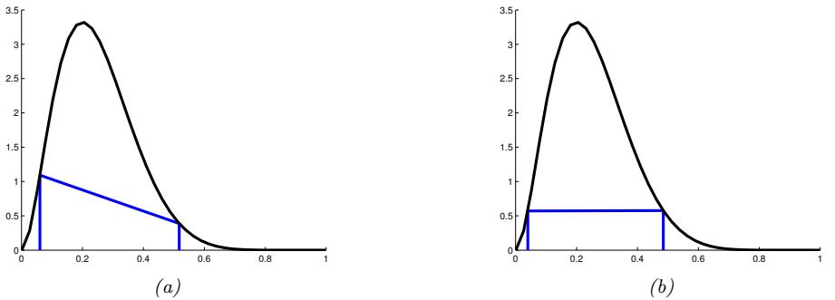
Figure 4.18: (a) Central interval and (b) HPD region for a Beta(3,9) posterior. The CI is (0.06, 0.52) and the HPD is (0.04, 0.48). Adapted from Figure 3.6 of [Hof09]. Generated by betaHPD.ipynb.

Note that ML-II is less likely to overfit than “regular” maximum likelihood, because there are typically fewer hyper-parameters ↼ than there are parameters ω. See the sequel to this book, [Mur23], for details.

4.6.6 Credible intervals

A posterior distribution is (usually) a high dimensional object that is hard to visualize and work with. A common way to summarize such a distribution is to compute a point estimate, such as the posterior mean or mode, and then to compute a credible interval, which quantifies the uncertainty associated with that estimate. (A credible interval is not the same as a confidence interval, which is a concept from frequentist statistics which we discuss in Section 4.7.4.)

More precisely, we define a 100(1 ↑ ϱ)% credible interval to be a (contiguous) region C = (ω, u) (standing for lower and upper) which contains 1 ↑ ϱ of the posterior probability mass, i.e.,

\[C\_{\alpha}(\mathcal{D}) = (\ell, u) : P(\ell \le \theta \le u | \mathcal{D}) = 1 - \alpha \tag{4.192}\]

There may be many intervals that satisfy Equation (4.192), so we usually choose one such that there is (1↑ϱ)/2 mass in each tail; this is called a central interval. If the posterior has a known functional form, we can compute the posterior central interval using ^{ω = F →}1(ϱ/2) and ^{u = F →}1(1↑ϱ/2), where F is the cdf of the posterior, and F ^→1 is the inverse cdf. For example, if the posterior is Gaussian, ^p(ϖ|D) = ^N (0, 1), and ^ϱ = 0.05, then we have ^{ω =} !→1(ϱ/2) = ^↑1.96, and ^{u =} !→1(1 ^{↑ ϱ}/2) = 1.96, where ! denotes the cdf of the Gaussian. This is illustrated in Figure 2.2b. This justifies the common practice of quoting a credible interval in the form of µ ± 2ε, where µ represents the posterior mean, ε represents the posterior standard deviation, and 2 is a good approximation to 1.96.

In general, it is often hard to compute the inverse cdf of the posterior. In this case, a simple alternative is to draw samples from the posterior, and then to use a Monte Carlo approximation to the posterior quantiles: we simply sort the S samples, and find the one that occurs at location ϱ/S along the sorted list. As S ↔︎ ∈, this converges to the true quantile. See beta\_credible\_int\_demo.ipynb for a demo of this.

A problem with central intervals is that there might be points outside the central interval which have higher probability than points that are inside, as illustrated in Figure 4.18(a). This motivates

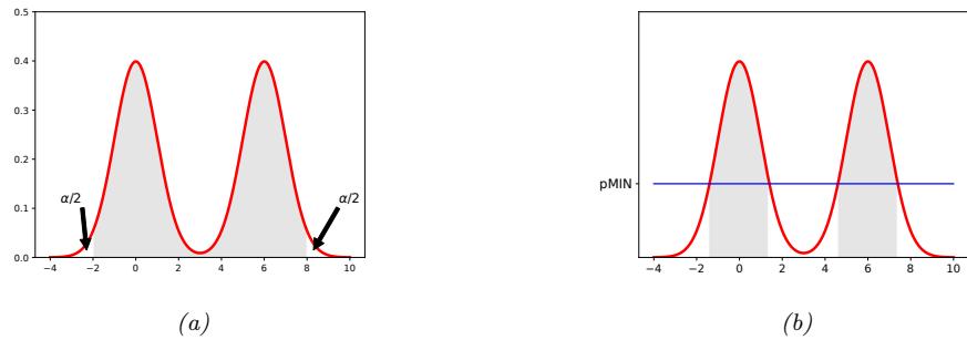
Figure 4.19: (a) Central interval and (b) HPD region for a hypothetical multimodal posterior. Adapted from Figure 2.2 of [Gel+04]. Generated by postDensityIntervals.ipynb.

an alternative quantity known as the highest posterior density or HPD region, which is the set of points which have a probability above some threshold. More precisely we find the threshold p^↓ on the pdf such that

\[1 - \alpha = \int\_{\theta: p(\theta|\mathcal{D}) > p^\*} p(\theta|\mathcal{D}) d\theta \tag{4.193}\]

and then define the HPD as

\[C\_{\alpha}(\mathcal{D}) = \{ \theta : p(\theta | \mathcal{D}) \ge p^\* \} \tag{4.194}\]

In 1d, the HPD region is sometimes called a highest density interval or HDI. For example, Figure 4.18(b) shows the 95% HDI of a Beta(3, 9) distribution, which is (0.04, 0.48). We see that this is narrower than the central interval, even though it still contains 95% of the mass; furthermore, every point inside of it has higher density than every point outside of it.

For a unimodal distribution, the HDI will be the narrowest interval around the mode containing 95% of the mass. To see this, imagine “water filling” in reverse, where we lower the level until 95% of the mass is revealed, and only 5% is submerged. This gives a simple algorithm for computing HDIs in the 1d case: simply search over points such that the interval contains 95% of the mass and has minimal width. This can be done by 1d numerical optimization if we know the inverse CDF of the distribution, or by search over the sorted data points if we have a bag of samples (see betaHPD.ipynb for some code).

If the posterior is multimodal, the HDI may not even be a connected region: see Figure 4.19(b) for an example. However, summarizing multimodal posteriors is always di”cult.

4.6.7 Bayesian machine learning

So far, we have focused on unconditional models of the form p(y|ω). In supervised machine learning, we use conditional models of the form p(y|x, ω). The posterior over the parameters is now p(ω|D), where D = {(xn, yn) : n =1: N}. Computing this posterior can be done using the principles we have already discussed. This approach is called Bayesian machine learning, since we are “being Bayesian” about the model parameters.

4.6.7.1 Plugin approximation

Once we have computed the posterior over the parameters, we can compute the posterior predictive distribution over outputs given inputs by marginalizing out the unknown parameters:

\[p(\mathbf{y}|\mathbf{z}, \mathcal{D}) = \int p(\mathbf{y}|\mathbf{z}, \boldsymbol{\theta}) p(\boldsymbol{\theta}|\mathcal{D}) d\boldsymbol{\theta} \tag{4.195}\]

Of course, computing this integral is often intractable. A very simple approximation is to assume there is just a single best model, ωˆ, such as the MLE. This is equivalent to approximating the posterior as an infinitely narrow, but infinitely tall, “spike” at the chosen value. We can write this as follows:

\[p(\boldsymbol{\theta}|\mathcal{D}) = \delta(\boldsymbol{\theta} - \hat{\boldsymbol{\theta}}) \tag{4.196}\]

where ↽ is the Dirac delta function (see Section 2.6.5). If we use this approximation, then the predictive distribution can be obtained by simply “plugging in” the point estimate into the likelihood:

\[p(\boldsymbol{y}|\boldsymbol{x},\mathcal{D}) = \int p(\boldsymbol{y}|\boldsymbol{x},\boldsymbol{\theta})p(\boldsymbol{\theta}|\mathcal{D})d\boldsymbol{\theta} \approx \int p(\boldsymbol{y}|\boldsymbol{x},\boldsymbol{\theta})\delta(\boldsymbol{\theta}-\hat{\boldsymbol{\theta}})d\boldsymbol{\theta} = p(\boldsymbol{y}|\boldsymbol{x},\hat{\boldsymbol{\theta}})\tag{4.197}\]

This follows from the sifting property of delta functions (Equation (2.129)).

The approach in Equation (4.197) is called a plug-in approximation. This approach is equivalent to the standard approach used in most of machine learning, in which we first fit the model (i.e. compute a point estimate ωˆ) and then use it to make predicitons. However, the standard (plug-in) approach can su!er from overfitting and overconfidence, as we discussed in Section 1.2.3. The fully Bayesian approach avoids this by marginalizing out the parameters, but can be expensive. Fortunately, even simple approximations, in which we average over a few plausible parameter values, can improve performance. We give some examples of this below.

4.6.7.2 Example: scalar input, binary output

Suppose we want to perform binary classification, so y → {0, 1}. We will use a model of the form

\[p(y|x; \theta) = \text{Ber}(y|\sigma(\mathbf{w}^\mathsf{T}x + b))\tag{4.198}\]

where

\[ \sigma(a) \stackrel{\Delta}{=} \frac{e^a}{1 + e^a} \tag{4.199} \]

is the sigmoid or logistic function which maps R ↔︎ [0, 1], and Ber(y|µ) is the Bernoulli distribution with mean µ (see Section 2.4 for details). In other words,

\[p(y=1|\mathbf{z}; \boldsymbol{\theta}) = \sigma(\boldsymbol{w}^{\mathsf{T}}\boldsymbol{x} + b) = \frac{1}{1 + e^{-(\mathbf{w}^{\mathsf{T}}\boldsymbol{x} + b)}}\tag{4.200}\]

This model is called logistic regression. (We discuss this in more detail in Chapter 10.)

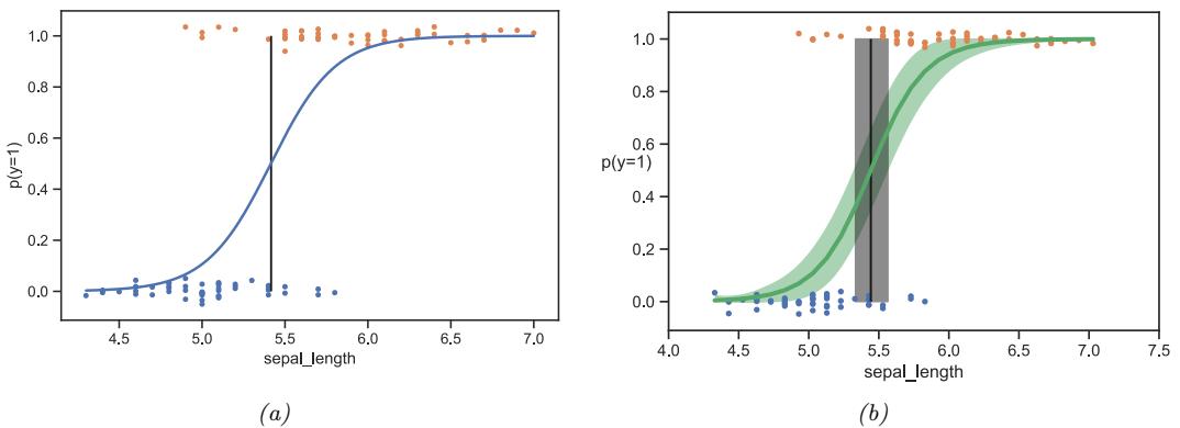
Figure 4.20: (a) Logistic regression for classifying if an Iris flower is Versicolor (y = 1) or setosa (y = 0) using a single input feature x corresponding to sepal length. Labeled points have been (vertically) jittered to avoid overlapping too much. Vertical line is the decision boundary. Generated by logreg\_iris\_1d.ipynb. (b) Same as (a) but showing posterior distribution. Adapted from Figure 4.4 of [Mar18]. Generated by logreg\_iris\_bayes\_1d\_pymc3.ipynb.

Let us apply this model to the task of determining if an iris flower is of type Setosa or Versicolor, yⁿ → {0, 1}, given information about the sepal length, xn. (See Section 1.2.1.1 for a description of the iris dataset.)

We first fit a 1d logistic regression model of the following form

\[p(y=1|x; \theta) = \sigma(b+wx) \tag{4.201}\]

to the dataset D = {(xn, yn)} using maximum likelihood estimation. (See Section 10.2.3 for details on how to compute the MLE for this model.) Figure 4.20a shows the plugin approximation to the posterior predictive, ^p(^y = 1|x, ^ωˆ), where ^ωˆ is the MLE of the parameters. We see that we become more confident that the flower is of type Versicolor as the sepal length gets larger, as represented by the sigmoidal (S-shaped) logistic function.

The decision boundary is defined to be the input value ^x↓ where ^p(^y = 1|x↓; ^ωˆ)=0.5. We can solve for this value as follows:

\[ \sigma(b + wx^\*) = \frac{1}{1 + e^{-(b + wx^\*)}} = \frac{1}{2} \tag{4.202} \]

\[b + wx^\* = 0\tag{4.203}\]

\[x^\* = -\frac{b}{w} \tag{4.204}\]

From Figure 4.20a, we see that x^↓ ↖ 5.5 cm.

However, the above approach does not model the uncertainty in our estimate of the parameters, and therefore ignores the induced uncertainty in the output probabilities, and the location of the decision boundary. To capture this additional uncertainty, we can use a Bayesian approach to approximate

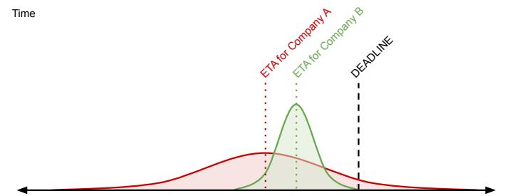
Figure 4.21: Distribution of arrival times for two di!erent shipping companies. ETA is the expected time of arrival. A’s distribution has greater uncertainty, and may be too risky. From https: // bit. ly/ 39bc4XL . Used with kind permission of Brendan Hasz.

the posterior p(ω|D). (See Section 10.5 for details.) Given this, we can approximate the posterior predictive distribution using a Monte Carlo approximation:

\[p(y=1|x, \mathcal{D}) \approx \frac{1}{S} \sum\_{s=1}^{S} p(y=1|x, \mathbf{\theta}^s) \tag{4.205}\]

where ^{ωs ⇒ p}(ω|D) is a posterior sample. Figure 4.20b plots the mean and 95% credible interval of this function. We see that there is now a range of predicted probabilities for each input. We can also compute a distribution over the location of the decision boundary by using the Monte Carlo approximation

\[p(x^\*|\mathcal{D}) \approx \frac{1}{S} \sum\_{s=1}^S \delta \left( x^\* - (-\frac{b^s}{w^s}) \right) \tag{4.206}\]

where (b^s, w^s) = ω^s. The 95% credible interval for this distribution is shown by the “fat” vertical line in Figure 4.20b.

Although carefully modeling our uncertainty may not matter for this application, it can be important in risk-sensitive applications, such as health care and finance, as we discuss in Chapter 5.

4.6.7.3 Example: binary input, scalar output

Now suppose we want to predict the delivery time for a package, y → R, if shipped by company A vs B. We can encode the company id using a binary feature x → {0, 1}, where x = 0 means company A and x = 1 means company B. We will use the following discriminative model for this problem:

\[p(y|x,\theta) = N(y|\mu\_x, \sigma\_x^2) \tag{4.207}\]

where ^N (y|µ, ^ε2) is the Gaussian distribution

\[\mathcal{N}(y|\mu, \sigma^2) \triangleq \frac{1}{\sqrt{2\pi\sigma^2}} e^{-\frac{1}{2\sigma^2}(y-\mu)^2} \tag{4.208}\]

and ω = (µ0, µ1, ε0, ε1) are the parameters of the model. We can fit this model using maximum likelihood estimation as we discuss in Section 4.2.5; alternatively, we can adopt a Bayesian approach, as we discuss in Section 4.6.4.

The advantage of the Bayesian approach is that by capturing uncertainty in the parameters ω, we also capture uncertainty in our forecasts ^p(y|x, ^D), whereas using a plug-in approximation ^p(y|x, ^ωˆ) would underestimate this uncertainty. For example, suppose we have only used each company once, so our training set has the form D = {(x¹ = 0, y¹ = 15),(x² = 1, y² = 20)}. As we show in Section 4.2.5, the MLE for the means will be the empirical means, µˆ⁰ = 15 and µˆ¹ = 20, but the MLE for the standard deviations will be zero, εˆ⁰ = εˆ¹ = 0, since we only have a single sample from each “class”. The resulting plug-in prediction will therefore not capture any uncertainty.

To see why modeling the uncertainty is important, consider Figure 4.21. We see that the expected time of arrival (ETA) for company A is less than for company B; however, the variance of A’s distribution is larger, which makes it a risky choice if you want to be confident the package will arrive by the specified deadline. (For more details on how to choose optimal actions in the presence of uncertainty, see Chapter 5.)

Of course, the above example is extreme, because we assumed we only had one example from each delivery company. However, this kind of problem occurs whenever we have few examples of a given kind of input, as can happen whenever the data has a long tail of novel patterns, such as a new combination of words or categorical features.

4.6.7.4 Scaling up

The above examples were both extremely simple, involving 1d input and 1d output, and just 2–4 parameters. Most practical problems involve high dimensional inputs, and sometimes high dimensional outputs, and therefore use models with lots of parameters. Unfortunately, computing the posterior, p(ω|D), and the posterior predictive, p(y|x, D), can be computationally challenging in such cases. We discuss this issue in Section 4.6.8.

4.6.8 Computational issues

Given a likelihood p(D|ω) and a prior p(ω), we can compute the posterior p(ω|D) using Bayes’ rule. However, actually performing this computation is usually intractable, except for simple special cases, such as conjugate models (Section 4.6.1), or models where all the latent variables come from a small finite set of possible values. We therefore need to approximate the posterior. There are a large variety of methods for performing approximate posterior inference, which trade o! accuracy, simplicity, and speed. We briefly discuss some of these algorithms below, but go into more detail in the sequel to this book, [Mur23]. (See also [MFR20] for a review of various approximate inference methods, starting with Bayes’ original method in 1763.)

As a running example, we will use the problem of approximating the posterior of a beta-Bernoulli model. Specifically, the goal is to approximate

\[p(\theta|\mathcal{D}) \propto \left[ \prod\_{n=1}^{N} \text{Bin}(y\_n|\theta) \right] \text{Beta}(\theta|1, 1) \tag{4.209}\]

where D consists of 10 heads and 1 tail (so the total number of observations is N = 11), and we use a uniform prior. Although we can compute this posterior exactly (see Figure 4.22), using the

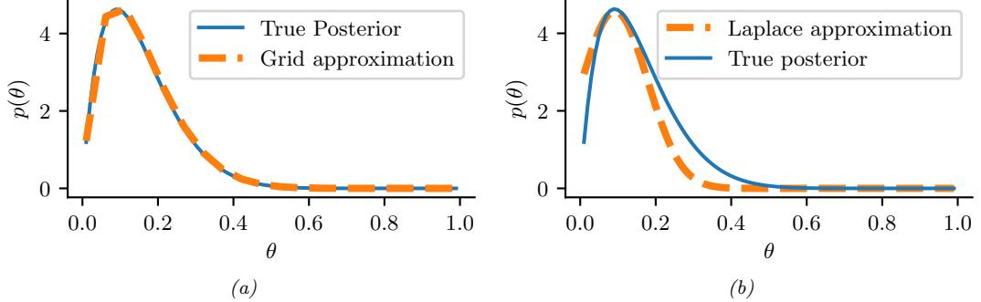
Figure 4.22: Approximating the posterior of a beta-Bernoulli model. (a) Grid approximation using 20 grid points. (b) Laplace approximation. Generated by laplace\_approx\_beta\_binom\_jax.ipynb.

method discussed in Section 4.6.2, this serves as a useful pedagogical example since we can compare the approximation to the exact answer. Also, since the target distribution is just 1d, it is easy to visualize the results. (Note, however, that the problem is not completely trivial, since the posterior is highly skewed, due to the use of an imbalanced sample of 10 heads and 1 tail.)

4.6.8.1 Grid approximation

The simplest approach to approximate posterior inference is to partition the space of possible values for the unknowns into a finite set of possibilities, call them ω1,…, ωK, and then to approximate the posterior by brute-force enumeration, as follows:

\[p(\boldsymbol{\theta} = \boldsymbol{\theta}\_k | \mathcal{D}) \approx \frac{p(\mathcal{D} | \boldsymbol{\theta}\_k) p(\boldsymbol{\theta}\_k)}{p(\mathcal{D})} = \frac{p(\mathcal{D} | \boldsymbol{\theta}\_k) p(\boldsymbol{\theta}\_k)}{\sum\_{k'=1}^K p(\mathcal{D}, \boldsymbol{\theta}\_{k'})} \tag{4.210}\]

This is called a grid approximation. In Figure 4.22a, we illustrate this method applied to our 1d problem. We see that it is easily able to capture the skewed posterior. Unfortunately, this approach does not scale to problems in more than 2 or 3 dimensions, because the number of grid points grows exponentially with the number of dimensions.

4.6.8.2 Quadratic (Laplace) approximation

In this section, we discuss a simple way to approximate the posterior using a multivariate Gaussian; this is known as a Laplace approximation or a quadratic approximation (see e.g., [TK86; RMC09]).

To derive this, suppose we write the posterior as follows:

\[p(\boldsymbol{\theta}|\mathcal{D}) = \frac{1}{Z}e^{-\mathcal{E}(\boldsymbol{\theta})} \tag{4.211}\]

where E(ω) = ↑ log p(ω, D) is called an energy function, and Z = p(D) is the normalization constant. Performing a Taylor series expansion around the mode ωˆ (i.e., the lowest energy state) we get

\[\mathcal{E}(\boldsymbol{\theta}) \approx \mathcal{E}(\hat{\boldsymbol{\theta}}) + (\boldsymbol{\theta} - \hat{\boldsymbol{\theta}})^{\mathsf{T}} \boldsymbol{g} + \frac{1}{2} (\boldsymbol{\theta} - \hat{\boldsymbol{\theta}})^{\mathsf{T}} \mathbf{H} (\boldsymbol{\theta} - \hat{\boldsymbol{\theta}}) \tag{4.212}\]

where g is the gradient at the mode, and H is the Hessian. Since ωˆ is the mode, the gradient term is zero. Hence

\[\hat{p}(\boldsymbol{\theta}, \mathcal{D}) = e^{-\mathcal{E}(\hat{\boldsymbol{\theta}})} \exp\left[ -\frac{1}{2} (\boldsymbol{\theta} - \hat{\boldsymbol{\theta}})^{\mathsf{T}} \mathbf{H}(\boldsymbol{\theta} - \hat{\boldsymbol{\theta}}) \right] \tag{4.213}\]

\[\hat{p}(\boldsymbol{\theta}|\mathcal{D}) = \frac{1}{Z}\hat{p}(\boldsymbol{\theta}, \mathcal{D}) = \mathcal{N}(\boldsymbol{\theta}|\hat{\boldsymbol{\theta}}, \mathbf{H}^{-1})\tag{4.214}\]

\[Z = e^{-\mathcal{E}(\hat{\theta})} (2\pi)^{D/2} |\mathbf{H}|^{-\frac{1}{2}} \tag{4.215}\]

The last line follows from normalization constant of the multivariate Gaussian.

The Laplace approximation is easy to apply, since we can leverage existing optimization algorithms to compute the MAP estimate, and then we just have to compute the Hessian at the mode. (In high dimensional spaces, we can use a diagonal approximation.)

In Figure 4.22b, we illustrate this method applied to our 1d problem. Unfortunately we see that it is not a particularly good approximation. This is because the posterior is skewed, whereas a Gaussian is symmetric. In addition, the parameter of interest lies in the constrained interval ϖ → [0, 1], whereas the Gaussian assumes an unconstrained space, ω → R. Fortunately, we can solve this latter problem by using a change of variable. For example, in this case we can apply the Laplace approximation to ϱ = logit(ϖ). This is a common trick to simplify the job of inference.

4.6.8.3 Variational approximation

In Section 4.6.8.2, we discussed the Laplace approximation, which uses an optimization procedure to find the MAP estimate, and then approximates the curvature of the posterior at that point based on the Hessian. In this section, we discuss variational inference (VI), which is another optimization-based approach to posterior inference, but which has much more modeling flexibility (and thus can give a much more accurate approximation).

VI attempts to approximate an intractable probability distribution, such as p(ω|D), with one that is tractable, q(ω), so as to minimize some discrepancy D between the distributions:

\[q^\* = \operatorname\*{argmin}\_{q \in \mathcal{Q}} D(q, p) \tag{4.216}\]

where Q is some tractable family of distributions (e.g., multivariate Gaussian). If we define D to be the KL divergence (see Section 6.2), then we can derive a lower bound to the log marginal likelihood; this quantity is known as the evidence lower bound or ELBO. By maximizing the ELBO, we can improve the quality of the posterior approximation. See the sequel to this book, [Mur23], for details.

4.6.8.4 Markov Chain Monte Carlo (MCMC) approximation

Although VI is a fast, optimization-based method, it can give a biased approximation to the posterior, since it is restricted to a specific function form q → Q. A more flexible approach is to use a nonparametric approximation in terms of a set of samples, ^q(ω) ↖ ¹ S $^{S s}=1 ↽(^{ω ↑ ωs}). This is called a Monte Carlo approximation to the posterior. The key issue is how to create the posterior samples ^{ωs ⇒ p}(ω|D) ^e“ciently, without having to evaluate the normalization constant ^p(D) = ^{H p}(ω, ^D)dω. A common approach to this problem is known as Markov chain Monte Carlo or MCMC. If we augment this algorithm with gradient-based information, derived from ̸ log p(ω, D), we can

significantly speed up the method; this is called Hamiltonian Monte Carlo or HMC. See the sequel to this book, [Mur23], for details.

4.7 Frequentist statistics *

The approach to statistical inference that we described in Section 4.6 is called Bayesian statistics. It treats parameters of models just like any other unknown random variable, and applies the rules of probability theory to infer them from data. Attempts have been made to devise approaches to statistical inference that avoid treating parameters like random variables, and which thus avoid the use of priors and Bayes rule. This alternative approach is known as frequentist statistics, classical statistics or orthodox statistics.

The basic idea (formalized in Section 4.7.1) is to represent uncertainty by calculating how a quantity estimated from data (such as a parameter or a predicted label) would change if the data were changed. It is this notion of variation across repeated trials that forms the basis for modeling uncertainty used by the frequentist approach. By contrast, the Bayesian approach views probability in terms of information rather than repeated trials. This allows the Bayesian to compute the probability of one-o! events, as we discussed in Section 2.1.1. Perhaps more importantly, the Bayesian approach avoids certain paradoxes that plague the frequentist approach (see Section 4.7.5 and Section 5.5.4). These pathologies led the famous statistician George Box to say:

I believe that it would be very di”cult to persuade an intelligent person that current [frequentist] statistical practice was sensible, but that there would be much less di”culty with an approach via likelihood and Bayes’ theorem. — George Box, 1962 (quoted in [Jay76]).

Nevertheless, it is useful to be familiar with frequentist statistics, since it is widely used, and has some key concepts that are useful even for Bayesians [Rub84].

4.7.1 Sampling distributions

In frequentist statistics, uncertainty is not represented by the posterior distribution of a random variable, but instead by the sampling distribution of an estimator.

The term “estimator” is defined in the section on decision theory in Section 5.1, but in brief, an estimator ↽ : D ↔︎ A is a decision procedure that specifies what action to take given some observed data. The action could be to predict a class label, or the next observation, or to predict the unknown parameters. In the latter case, the estimator is often denoted by ωˆ, but this notation is ambiguous, since it looks like it represents a parameter vector rather than a function. So instead we will use the notation #ˆ . This function could compute the MLE, or the method of moments estimate, etc. The output of this function, when applied to a specific dataset of size ^N, is denote ^{ωˆ =} #^ˆ (D), where D = {x1,…, x^N }.

The key idea in frequentist statistics is to view the data D as a random variable, and the parameters from which the data are drawn, ^ω↓, as a fixed but unknown constant. Thus ^{ωˆ =} #^ˆ (D) is a random variable, and its distribution is known as the sampling distribution of the estimator. To understand what thus means, suppose we create S di!erent datasets, each of the form

\[\mathcal{D}^{(s)} = \{ \mathbf{x}\_n \sim p(\mathbf{x}\_n | \theta^\*) : n = 1 : N \} \tag{4.217}\]

We denote this by ^D(s) ^{⇒ ω↓} for brevity. Now we apply the estimator to each ^D(s) to get a set of estimates, {ωˆ(D(s) )}. As we let S ↔︎ ∈, the distribution induced by this set is the sampling distribution of the estimator. More precisely, we have

\[\text{SamplingDist}(\hat{\Theta}, \theta^\*) = \text{PushThreshold}(p(\tilde{\mathcal{D}} | \theta^\*), \hat{\Theta}) \tag{4.218}\]

where we push the data distribution through the estimator function to induce a distribution of estimates. In some cases, we can compute the sampling distribution analytically, as we discuss in Section 4.7.2, although typically we need to approximate it by Monte Carlo, as we discuss in Section 4.7.3.

4.7.2 Gaussian approximation of the sampling distribution of the MLE

The most common estimator is the MLE. When the sample size becomes large, the sampling distribution of the MLE for certain models becomes Gaussian. This is known as the asymptotic normality of the sampling distribution. More formally, we have the following result:

Theorem 4.7.1. If the parameters are identifiable, then

\[\text{SamplingDist}(\hat{\Theta}^{\text{mle}}, \theta^\*) \to \mathcal{N}(\cdot | \theta^\*, (N\mathbf{F}(\theta^\*))^{-1})\tag{4.219}\]

where F(ω↓) is the Fisher information matrix, defined in Equation (4.220).

Equivalently, the above result says that the distribution of -NF(ω↓)(ω^{ˆ ↑ ω}↓) approaches ^N (0, ^I), where ^{ωˆ =} #^ˆ mle(D˜ ).

The Fisher information matrix measures the amount of curvature of the log-likelihood surface at its peak, as we show below. More formally, the Fisher information matrix (FIM) is defined to be the covariance of the gradient of the log likelihood (also called the score function):

\[\mathbf{F}(\boldsymbol{\theta}) \triangleq \mathbb{E}\_{\mathbf{z} \sim p(\mathbf{z}|\boldsymbol{\theta})} \left[ \nabla \log p(\mathbf{z}|\boldsymbol{\theta}) \nabla \log p(\mathbf{z}|\boldsymbol{\theta})^{\mathsf{T}} \right] \tag{4.220}\]

Hence the (i, j)’th entry has the form

\[F\_{ij} = \mathbb{E}\_{\mathbf{z} \sim \theta} \left[ \left( \frac{\partial}{\partial \theta\_i} \log p(\mathbf{z}|\theta) \right) \left( \frac{\partial}{\partial \theta\_j} \log p(\mathbf{z}|\theta) \right) \right] \tag{4.221}\]

One can show the following result.

Theorem 4.7.2. If log p(x|ω) is twice di!erentiable, and under certain regularity conditions, the FIM is equal to the expected Hessian of the NLL, i.e.,

\[\mathbf{F}\_{ij} = -\mathbb{E}\_{x \sim \theta} \left[ \frac{\partial^2}{\partial \theta\_i \theta\_j} \log p(x|\theta) \right] \tag{4.222}\]

If we replace the expectation over x with the observed value, to get the empirical FIM, we see this is equal to the Hessian of the NLL. This helps us understand the result in Equation (4.219): a log-likelihood function with high curvature (large Hessian) will result in a low variance estimate, since the parameters are “well determined” by the data, and hence robust to repeated sampling.

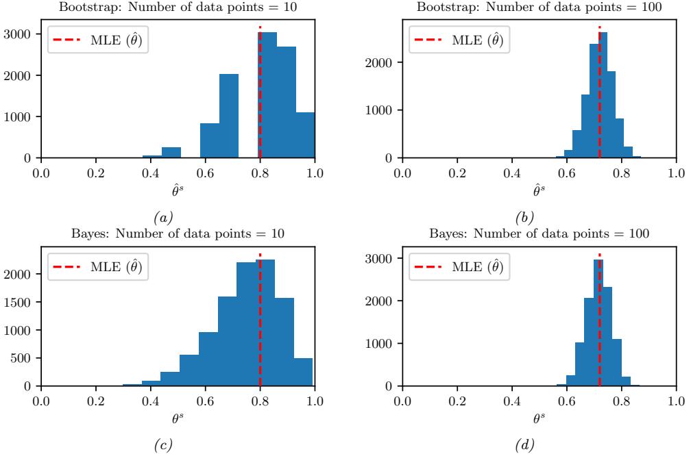
Figure 4.23: Bootstrap (top row) vs Bayes (bottom row). The N data cases were generated from Ber(ε = 0.7). Left column: N = 10. Right column: N = 100. (a-b) A bootstrap approximation to the sampling distribution of the MLE for a Bernoulli distribution. We show the histogram derived from B = 10, 000 bootstrap samples. (c-d) Histogram of 10,000 samples from the posterior distribution using a uniform prior. Generated by bootstrap\_demo\_bernoulli.ipynb.

In the scalar case, we have that V ^{ˆϖ ↑ ϖ↓ ↔︎ 1} NF (ϱ↑) . The square root of the variance of the sampling distribution of an estimator is known as its standard error or se. Hence we can say that the distribution of ^{ϱ ˆ}→ϱ^↑ se approaches N (0, 1). In practice the se is not known, but it can be estimated from data. For example, suppose ^{Xn ⇒} Ber(ϖ↓) and let ^{ˆϖ = 1} N $^{N n}=1 Xⁿ be the MLE. The standard error is se = ^J V ˆϖ ⁼ -ϖ↓(1 ^{↑ ϖ}↓)/N, so the estimated standard error is ˆse = ^Gˆϖ(1 ^{↑ ˆ}ϖ)/N.

4.7.3 Bootstrap approximation of the sampling distribution of any estimator

In cases where the estimator is a complex function of the data (e.g., not just an MLE), or when the sample size is small, we can approximate its sampling distribution using a Monte Carlo technique known as the bootstrap.

The idea is simple. If we knew the true parameters ω↓, we could generate many (say S) fake datasets, each of size ^N, from the true distribution, using ^D˜ (s) ⁼ {x^{n ⇒ p}(xn|ω↓) : ⁿ =1: ^N}. We could then compute our estimate from each sample, ^ωˆ^{s =} #^ˆ (D˜ (s) ) and use the empirical distribution of the resulting ωˆ^s as our estimate of the sampling distribution, as in Equation (4.218). Since ω^↓ is

unknown, we can use the dataset itself as an empirical approximation to p(xn|ω↓). More precisely, the idea is to generate each D˜(s) by sampling N data points with replacement from the original dataset. (If we sampled N times without replacement, we would just recover the original dataset.) This is like “lifting yourself up from your own bootstraps”, since we use the observed data sample to make new hypothetical data samples.6

Figure 4.23(a-b) shows an example where we compute the sampling distribution of the MLE for a Bernoulli using the bootstrap. When N = 10, we see that the sampling distribution is asymmetric, and therefore quite far from Gaussian, but when N = 100, the distribution looks more Gaussian, as theory suggests (see Section 4.7.2).

The number of unique data points in a bootstrap sample is just 0.632 ↓ N, on average. (To see this, note that the probability an item is picked at least once is (1 ^↑ (1 ^{↑ 1}/N)^N ), which approaches 1 ^{↑ e}→¹ ↖ 0.632 for large ^N.) However, there are more sophisticated versions of bootstrap that improve on this (see e.g., [Efr87; EH16]).

4.7.3.1 Bootstrap is a “poor man’s” posterior

A natural question is: what is the connection between the parameter estimates ^ωˆ^{s =} #ˆ(D(s) ) computed by the bootstrap and parameter values sampled from the posterior, ^{ωs ⇒ p}(·|D)? Conceptually they are quite di!erent. But in the common case that the estimator is MLE and the prior is not very strong, they can be quite similar. For example, Figure 4.23(c-d) shows an example where we compute the posterior using a uniform Beta(1,1) prior, and then sample from it. We see that the posterior and the sampling distribution are quite similar. So one can think of the bootstrap distribution as a “poor man’s” posterior [HTF01, p235].

However, perhaps surprisingly, bootstrap can be slower than posterior sampling. The reason is that the bootstrap has to generate S sampled datasets, and then fit a model to each one. By contrast, in posterior sampling, we only have to “fit” a model once given a single dataset. (Some methods for speeding up the bootstrap when applied to massive data sets are discussed in [Kle+11].)

4.7.4 Confidence intervals

In frequentist statistics, we use the variability induced by the sampling distribution as a way to estimate uncertainty of a parameter estimate.

In particular, we define a 100(1 ↑ ϱ)% confidence interval for parameter ϖ as an estimator that returns an interval that captures the true parameter with probability at least 1 ↑ ϱ. Denote the estimator by I(D)=(ω(D), u(D)). The sampling distribution of this estimator is the distribution that is induced by sampling ^D˜ ^{⇒ ϖ↓} and then computing ^I(D˜ ). We require that

\[\Pr(\theta^\* \in I(\tilde{\mathcal{D}}) | \tilde{\mathcal{D}} \sim \theta^\*) \ge 1 - \alpha \tag{4.223}\]

It is common to set ϱ = 0.05, which yields a 95% CI. This means that, if we repeatedly sampled data, and compute ^I(D˜ ) for each such dataset, then about 95% of such intervals will contain the true parameter ϖ.

^6. This is called the non-parametric bootstrap. There is another variant, called the parametric bootstrap, in which we sample each ^D˜(s) from ^p(xn|!^ˆ (D)); this requires fitting a parametric model to the original data and then sampling from it.

Let us give an example. Suppose that ^{ˆϖ =} #^ˆ (D) is an estimator for some parameter with true but unknown value ^ϖ↓. Also, suppose that the sampling distribution of % ^{= ϖ↓ ↑ ˆϖ} is known. Let ↽ and ↽ denote its ϱ/2 and 1 ↑ ϱ/2 quantiles, so

\[\Pr(\underline{\delta} \le \Delta \le \overline{\delta}) = \Pr(\underline{\delta} \le \theta^\* - \hat{\theta} \le \overline{\delta}) = 1 - \alpha \tag{4.224}\]

Rearranging we get

\[\Pr(\hat{\theta} + \underline{\delta} \le \theta^\* \le \hat{\theta} + \overline{\delta}) = 1 - \alpha \tag{4.225}\]

Hence we can construct a 100(1 ↑ ϱ)% confidence interval as follows:

\[I(\mathcal{D}) = (L, U) = \left(\hat{\theta}(\mathcal{D}) + \underline{\delta}(\mathcal{D}), \hat{\theta}(\mathcal{D}) + \overline{\delta}(\mathcal{D})\right) \tag{4.226}\]

In some cases, we can analytically compute the sampling distribution of the above interval. However, it is more common to assume a Gaussian approximation to the sampling distribution, as in Section 4.7.2. In this case, we have ^ˆϖ ↖ ^N (ϖ↓, ˆse²). Hence we can compute an approximate CI using

\[I = (\hat{\theta} - z\_{\alpha/2}\hat{\mathbf{s}}\mathbf{e}, \hat{\theta} + z\_{\alpha/2}\hat{\mathbf{s}}\mathbf{e})\tag{4.227}\]

where z↽/² is the ϱ/2 quantile of the Gaussian cdf. If we set ϱ = 0.05, we have z↽/² = 1.96, which justifies the common approximation ^{ˆϖ ±} 2 ˆse.

If the Gaussian approximation is not a good one, we can use a bootstrap approximation (see Section 4.7.3). In particular, we sample ^S datasets from ^ˆϖ(D), and apply the estimator to each one to get ^ˆϖ(D(s) ); we then use the empirical distribution of ^ˆϖ(D) ^{↑ ˆ}ϖ(D(s) ) as an approximation to the sampling distribution of %. We can then use the ϱ/2 and 1 ↑ ϱ/2 quantiles of this distribution to derive the CI (see [Was04, p110] for details).

4.7.5 Caution: Confidence intervals are not credible

It is commonly believed that a 95% confidence interval I for a parameter estimate ϖ given data D means that the true parameter lies in this interval with probability 0.95, i.e, p(ϖ^↓ → I|D)=0.95). However, this quantity is what a Bayesian credible interval computes (Section 4.6.6), but is not what a frequentist confidence interval computes. Instead the frequentist approach just means that the procedure for generating CIs will contain the true value 95% of the time. That is, if we repeatedly sample datasets ^D˜ from ^ϖ↓, and compute their CIs to get ^I(D˜ ), then we have Pr(ϖ^{↓ → I}(D˜ )) = 0.95, as we explain in Section 4.7.4. Thus we see that these concepts are quite di!erent: In the frequentist approach, ϖ is treated as an unknown fixed constant, and the data is treated as random. In the Bayesian approach, we treat the data as fixed (since it is known) and the parameter as random (since it is unknown).

This counter-intuitive definition of confidence intervals can lead to bizarre results. Consider the following example from [Ber85, p11]. Suppose we draw two integers D = (y1, y2) from

\[p(y|\theta) = \begin{cases} \begin{array}{ll} 0.5 & \text{if } y = \theta \\ 0.5 & \text{if } y = \theta + 1 \\ 0 & \text{otherwise} \end{array} \tag{4.228}\]

If ϖ = 39, we would expect the following outcomes each with probability 0.25:

\[(39, 39), (39, 40), (40, 39), (40, 40) \tag{4.229}\]

Let m = min(y1, y2) and define the following interval:

\[[\ell(\mathcal{D}), u(\mathcal{D})] = [m, m] \tag{4.230}\]

For the above samples this yields

\[[39, 39], \quad [39, 39], \quad [39, 39], \quad [40, 40] \tag{4.231}\]

Hence Equation (4.230) is clearly a 75% CI, since 39 is contained in 3/4 of these intervals. However, if we observe D = (39, 40) then p(ϖ = 39|D)=1.0, so we know that ϖ must be 39, yet we only have 75% “confidence” in this fact. We see that the CI will “cover” the true parameter 75% of the time, if we compute multiple CIs from di!erent randomly sampled datasets, but if we just have a single observed dataset, and hence a single CI, then the frequentist “coverage” probability can be very misleading.

Another, less contrived, example is as follows. Suppose we want to estimate the parameter ϖ of a Bernoulli distribution. Let y = ¹ N $^{N n}=1 ^yn be the sample mean. The MLE is ^{ˆϖ = y}. An approximate 95% confidence interval for a Bernoulli parameter is ^{y ± 1}.96-y(1 ^{↑ y})/N (this is called a Wald interval and is based on a Gaussian approximation to the Binomial distribution; compare to Equation (4.128)). Now consider a single trial, where N = 1 and y¹ = 0. The MLE is 0, which overfits, as we saw in Section 4.5.1. But our 95% confidence interval is also (0, 0), which seems even worse. It can be argued that the above flaw is because we approximated the true sampling distribution with a Gaussian, or because the sample size was too small, or the parameter “too extreme”. However, the Wald interval can behave badly even for large N, and non-extreme parameters [BCD01]. By contrast, a Bayesian credible interval with a non-informative Je!reys prior behaves in the way we would expect.

Several more interesting examples, along with Python code, can be found at [Van14]. See also [Hoe+14; Mor+16; Lyu+20; Cha+19b], who show that many people, including professional statisticians, misunderstand and misuse frequentist confidence intervals in practice, whereas Bayesian credible intervals do not su!er from these problems.

4.7.6 The bias-variance tradeo!

An estimator is a procedure applied to data which returns an estimand. Let ωˆ() be the estimator, and ^ωˆ(D) be the estimand. In frequentist statistics, we treat the data as a random variable, drawn from some true but unknown distribution, ^p↓(D); this induces a distribution over the estimand, ^p↓(ωˆ(D)), known as the sampling distribution (see Section 4.7.1). In this section, we discuss two key properties of this distribution, its bias and its variance, which we define below.

4.7.6.1 Bias of an estimator

The bias of an estimator is defined as

\[\text{bias}(\hat{\theta}(\cdot)) \stackrel{\Delta}{=} \mathbb{E}\left[\hat{\theta}(\mathcal{D})\right] - \theta^\* \tag{4.232}\]

where ϖ^↓ is the true parameter value, and the expectation is wrt “nature’s distribution” p(D|ϖ↓). If the bias is zero, the estimator is called unbiased. For example, the MLE for a Gaussian mean is unbiased:

\[\text{bias}(\hat{\mu}) = \mathbb{E}\left[\overline{x}\right] - \mu = \mathbb{E}\left[\frac{1}{N}\sum\_{n=1}^{N} x\_n\right] - \mu = \frac{N\mu}{N} - \mu = 0\tag{4.233}\]

where x is the sample mean.

However, the MLE for a Gaussian variance, ε² mle = ¹ N $^{N n}=1(x^{n ↑}x)2, is not an unbiased estimator of ε². In fact, one can show (Exercise 4.7) that

\[\mathbb{E}\left[\sigma\_{\text{mle}}^2\right] = \frac{N-1}{N}\sigma^2\tag{4.234}\]

so the ML estimator slightly underestimates the variance. Intuitively, this is because we “use up” one of the data points to estimate the mean, so if we have a sample size of 1, we will estimate the variance to be 0. If, however, µ is known, the ML estimator is unbiased (see Exercise 4.8).

Now consider the following estimator

\[ \sigma\_{\rm unb}^2 \triangleq \frac{1}{N-1} \sum\_{n=1}^N (x\_n - \overline{x})^2 = \frac{N}{N-1} \sigma\_{\rm mle}^2 \tag{4.235} \]

This is an unbiased estimator, which we can easily prove as follows:

\[\mathbb{E}\left[\sigma\_{\text{umb}}^2\right] = \frac{N}{N-1}\mathbb{E}\left[\sigma\_{\text{mle}}^2\right] = \frac{N}{N-1}\frac{N-1}{N}\sigma^2 = \sigma^2\tag{4.236}\]

4.7.6.2 Variance of an estimator

It seems intuitively reasonable that we want our estimator to be unbiased. However, being unbiased is not enough. For example, suppose we want to estimate the mean of a Gaussian from D = {x1,…,x^N }. The estimator that just looks at the first data point, ^ˆϖ(D) = ^x1, is an unbiased estimator, but will generally be further from ϖ^↓ than the empirical mean x (which is also unbiased). So the variance of an estimator is also important.

We define the variance of an estimator as follows:

\[\mathbb{V}\left[\hat{\theta}\right] \stackrel{\scriptstyle \triangleq}{=} \mathbb{E}\left[\hat{\theta}^2\right] - \left(\mathbb{E}\left[\hat{\theta}\right]\right)^2\tag{4.237}\]

where the expectation is taken wrt p(D|ϖ↓). This measures how much our estimate will change as the data changes. We can extend this to a covariance matrix for vector valued estimators.

Intuitively we would like the variance of our estimator to be as small as possible. Therefore, a natural question is: how low can the variance go? A famous result, called the Cramer-Rao lower bound, provides a lower bound on the variance of any unbiased estimator. More precisely, let ^X1,…,X^{N ⇒ p}(X|ϖ↓) and ^{ˆϖ = ˆ}ϖ(x1,…,x^N ) be an unbiased estimator of ^ϖ↓. Then, under various smoothness assumptions on p(X|ϖ↓), we have V ˆϖ ^{∋ 1} NF (ϱ↑) , where F(ϖ↓) is the Fisher information matrix (Section 4.7.2). A proof can be found e.g., in [Ric95, p275].

It can be shown that the MLE achieves the Cramer Rao lower bound, and hence has the smallest asymptotic variance of any unbiased estimator. Thus MLE is said to be asymptotically optimal.

4.7.6.3 The bias-variance tradeo”

In this section, we discuss a fundamental tradeo! that needs to be made when picking a method for parameter estimation, assuming our goal is to minimize the mean squared error (MSE) of our estimate. Let ^{ˆϖ = ˆ}ϖ(D) denote the estimate, and ^{ϖ = E} ˆϖ denote the expected value of the estimate (as we vary D). (All expectations and variances are wrt p(D|ϖ↓), but we drop the explicit conditioning for notational brevity.) Then we have

\[\mathbb{E}\left[\left(\hat{\theta} - \theta^\*\right)^2\right] = \mathbb{E}\left[\left[\left(\hat{\theta} - \overline{\theta}\right) + \left(\overline{\theta} - \theta^\*\right)\right]^2\right] \tag{4.238}\]

\[=\mathbb{E}\left[\left(\hat{\theta}-\overline{\theta}\right)^{2}\right]+2(\overline{\theta}-\theta^{\*})\mathbb{E}\left[\hat{\theta}-\overline{\theta}\right]+(\overline{\theta}-\theta^{\*})^{2}\tag{4.239}\]

\[\mathbf{E} = \mathbb{E}\left[\left(\hat{\theta} - \overline{\theta}\right)^2\right] + (\overline{\theta} - \theta^\*)^2 \tag{4.240}\]

\[\mathbf{u} = \mathbb{V}\left[\hat{\theta}\right] + \text{bias}^2(\hat{\theta}) \tag{4.241}\]

In words,

\[\text{MSE} = \text{variance} + \text{bias}^2 \Bigg| \tag{4.242}\]

This is called the bias-variance tradeo” (see e.g., [GBD92]). What it means is that it might be wise to use a biased estimator, so long as it reduces our variance by more than the square of the bias, assuming our goal is to minimize squared error.

4.7.6.4 Example: MAP estimator for a Gaussian mean

Let us give an example, based on [Hof09, p79]. Suppose we want to estimate the mean of a Gaussian from ^x = (x1,…,x^N ). We assume the data is sampled from ^{xn ⇒ N} (ϖ^↓ = 1, ^ε2). An obvious estimate is the MLE. This has a bias of 0 and a variance of

\[\mathbb{V}\left[\overline{x}|\theta^\*\right] = \frac{\sigma^2}{N} \tag{4.243}\]

But we could also use a MAP estimate. In Section 4.6.4.2, we show that the MAP estimate under a Gaussian prior of the form ^N (ϖ0, ^ε2/20) is given by

\[\bar{x} \triangleq \frac{N}{N + \kappa\_0} \overline{x} + \frac{\kappa\_0}{N + \kappa\_0} \theta\_0 = w \overline{x} + (1 - w)\theta\_0 \tag{4.244}\]

where 0 ↘ w ↘ 1 controls how much we trust the MLE compared to our prior. The bias and variance are given by

\[\mathbb{E}\left[\bar{x}\right] - \theta^\* = w\theta^\* + (1 - w)\theta\_0 - \theta^\* = (1 - w)(\theta\_0 - \theta^\*)\tag{4.245}\]

\[\mathbb{V}\left[\bar{x}\right] = w^2 \frac{\sigma^2}{N} \tag{4.246}\]

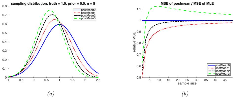
Figure 4.24: Left: Sampling distribution of the MAP estimate (equivalent to the posterior mean) under a ^N (ε⁰ = 0, ^ϑ2/⇁0) prior with di!erent prior strengths ⇁0. (If we set ⇁ = 0, the MAP estimate reduces to the MLE.) The data is ⁿ = 5 samples drawn from ^N (ε^↔︎ = 1, ^ϑ2 = 1). Right: MSE relative to that of the MLE versus sample size. Adapted from Figure 5.6 of [Hof09]. Generated by samplingDistributionGaussianShrinkage.ipynb.

So although the MAP estimate is biased (assuming w < 1), it has lower variance.

Let us assume that our prior is slightly misspecified, so we use ϖ⁰ = 0, whereas the truth is ϖ^↓ = 1. In Figure 4.24(a), we see that the sampling distribution of the MAP estimate for 2⁰ > 0 is biased away from the truth, but has lower variance (is narrower) than that of the MLE.

In Figure 4.24(b), we plot mse(x˜)/mse(x) vs N. We see that the MAP estimate has lower MSE than the MLE for 2⁰ → {1, 2}. The case 2⁰ = 0 corresponds to the MLE, and the case 2⁰ = 3 corresponds to a strong prior, which hurts performance because the prior mean is wrong. Thus we see that, provided the prior strength is properly “tuned”, a MAP estimate can outperform an ML estimate in terms of minimizing MSE.

4.7.6.5 Example: MAP estimator for linear regression

Another important example of the bias-variance tradeo! arises in ridge regression, which we discuss in Section 11.3. In brief, this corresponds to MAP estimation for linear regression under a Gaussian prior, ^p(w) = ^N (w|0, ^φ→1I) The zero-mean prior encourages the weights to be small, which reduces overfitting; the precision term, φ, controls the strength of this prior. Setting φ = 0 results in the MLE; using φ > 0 results in a biased estimate. To illustrate the e!ect on the variance, consider a simple example where we fit a 1d ridge regression model using 2 di!erent values of φ. Figure 4.25 on the left plots each individual fitted curve, and on the right plots the average fitted curve. We see that as we increase the strength of the regularizer, the variance decreases, but the bias increases.

See also Figure 4.26 where we give a cartoon sketch of the bias variance tradeo! in terms of model complexity.

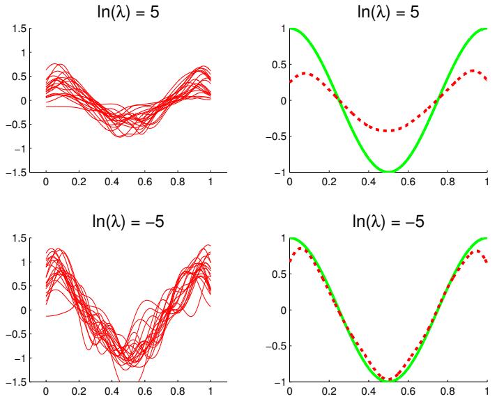
Figure 4.25: Illustration of bias-variance tradeo! for ridge regression. We generate 100 data sets from the true function, shown in solid green. Left: we plot the regularized fit for 20 di!erent data sets. We use linear regression with a Gaussian RBF expansion, with 25 centers evenly spread over the [0, 1] interval. Right: we plot the average of the fits, averaged over all 100 datasets. Top row: strongly regularized: we see that the individual fits are similar to each other (low variance), but the average is far from the truth (high bias). Bottom row: lightly regularized: we see that the individual fits are quite di!erent from each other (high variance), but the average is close to the truth (low bias). Adapted from [Bis06] Figure 3.5. Generated by biasVarModelComplexity3.ipynb.

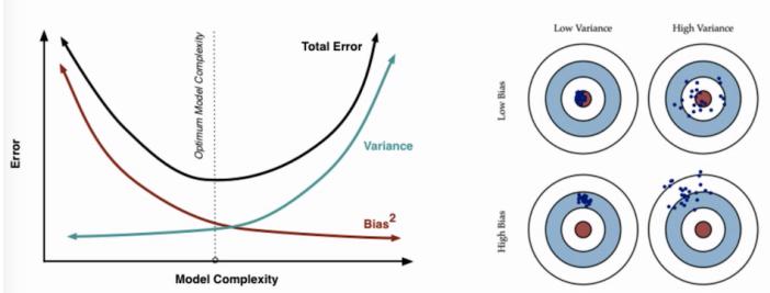
Figure 4.26: Cartoon illustration of the bias variance tradeo!. From http: // scott. fortmann-roe. com/ docs/ BiasVariance. html . Used with kind permission of Scott Fortmann-Roe.

4.7.6.6 Bias-variance tradeo” for classification

If we use 0-1 loss instead of squared error, the frequentist risk is no longer expressible as squared bias plus variance. In fact, one can show (Exercise 7.2 of [HTF09]) that the bias and variance combine multiplicatively. If the estimate is on the correct side of the decision boundary, then the bias is negative, and decreasing the variance will decrease the misclassification rate. But if the estimate is on the wrong side of the decision boundary, then the bias is positive, so it pays to increase the variance [Fri97a]. This little known fact illustrates that the bias-variance tradeo! is not very useful for classification. It is better to focus on expected loss, not directly on bias and variance. We can approximate the expected loss using cross validation, as we discuss in Section 4.5.5.

4.8 Exercises

Exercise 4.1 [MLE for the univariate Gaussian † ]

Show that the MLE for a univariate Gaussian is given by

\[ \hat{\mu} = \frac{1}{N} \sum\_{n=1}^{N} y\_n \tag{4.247} \]

\[ \hat{\sigma}^2 = \frac{1}{N} \sum\_{n=1}^{N} (y\_n - \hat{\mu})^2 \tag{4.248} \]

Exercise 4.2 [MAP estimation for 1D Gaussians † ]

(Source: Jaakkola.)

Consider samples x1,…,xⁿ from a Gaussian random variable with known variance ϑ² and unknown mean µ. We further assume a prior distribution (also Gaussian) over the mean, ^µ ↘ ^N (m, s²), with fixed mean ^m and fixed variance s². Thus the only unknown is µ.

• 1. Calculate the MAP estimate µˆMAP . You can state the result without proof. Alternatively, with a lot more work, you can compute derivatives of the log posterior, set to zero and solve.
• 2. Show that as the number of samples n increase, the MAP estimate converges to the maximum likelihood estimate.
• 3. Suppose n is small and fixed. What does the MAP estimator converge to if we increase the prior variance s²?
• 4. Suppose n is small and fixed. What does the MAP estimator converge to if we decrease the prior variance s²?

Exercise 4.3 [Gaussian posterior credible interval]

(Source: DeGroot.) Let ^X ↘ ^N (µ, ^ϑ2 = 4) where ^µ is unknown but has prior ^µ ↘ ^N (µ0, ^{ϑ2 0} = 9). The posterior after seeing ⁿ samples is ^µ ↘ ^N (µn, ^{ϑ2 n}). (This is called a credible interval, and is the Bayesian analog of a confidence interval.) How big does n have to be to ensure

\[p(\ell \le \mu\_n \le u | D) \ge 0.95 \tag{4.249}\]

where (,, u) is an interval (centered on µn) of width 1 and D is the data? Hint: recall that 95% of the probability mass of a Gaussian is within ±1.96ϑ of the mean.

Exercise 4.4 [BIC for Gaussians † ]

(Source: Jaakkola.)

The Bayesian information criterion (BIC) is a penalized log-likelihood function that can be used for model selection. It is defined as

\[BIC = \log p(\mathcal{D}|\hat{\theta}\_{ML}) - \frac{d}{2}\log(N) \tag{4.250}\]

where d is the number of free parameters in the model and N is the number of samples. In this question, we will see how to use this to choose between a full covariance Gaussian and a Gaussian with a diagonal covariance. Obviously a full covariance Gaussian has higher likelihood, but it may not be “worth” the extra parameters if the improvement over a diagonal covariance matrix is too small. So we use the BIC score to choose the model.

We can write

\[\log p(\mathcal{D}|\hat{\Sigma}, \hat{\mu}) = -\frac{N}{2} \text{tr}\left(\hat{\Sigma}^{-1}\hat{\mathbf{S}}\right) - \frac{N}{2} \log(|\hat{\Sigma}|) \tag{4.251}\]

\[\hat{\mathbf{S}} = \frac{1}{N} \sum\_{i=1}^{N} (\mathbf{x}\_i - \overline{\mathbf{x}})(\mathbf{x}\_i - \overline{\mathbf{x}})^T \tag{4.252}\]

where Sˆ is the scatter matrix (empirical covariance), the trace of a matrix is the sum of its diagonals, and we have used the trace trick.

• 1. Derive the BIC score for a Gaussian in D dimensions with full covariance matrix. Simplify your answer as much as possible, exploiting the form of the MLE. Be sure to specify the number of free parameters d.
• 2. Derive the BIC score for a Gaussian in D dimensions with a diagonal covariance matrix. Be sure to specify the number of free parameters d. Hint: for the digaonal case, the ML estimate of ! is the same as !ˆ ML except the o”-diagonal terms are zero:

\[ \hat{\Sigma}\_{diag} = \text{diag}(\hat{\Sigma}\_{ML}(1,1), \dots, \hat{\Sigma}\_{ML}(D,D)) \tag{4.253} \]

Exercise 4.5 [BIC for a 2d discrete distribution]

(Source: Jaakkola.)

Let x ⇒ {0, 1} denote the result of a coin toss (x = 0 for tails, x = 1 for heads). The coin is potentially biased, so that heads occurs with probability ε1. Suppose that someone else observes the coin flip and reports to you the outcome, y. But this person is unreliable and only reports the result correctly with probability ε2; i.e., p(y|x, ε2) is given by

\[\begin{array}{c|cc} & y=0 & y=1 \\ \hline x=0 & \theta\_2 & 1-\theta\_2 \\ x=1 & 1-\theta\_2 & \theta\_2 \\ \end{array}\]

Assume that ε² is independent of x and ε1.

• 1. Write down the joint probability distribution p(x, y|ω) as a 2 → 2 table, in terms of ω = (ε1, ε2).
• 2. Suppose have the following dataset: x = (1, 1, 0, 1, 1, 0, 0), y = (1, 0, 0, 0, 1, 0, 1). What are the MLEs for ε¹ and ε2? Justify your answer. Hint: note that the likelihood function factorizes,

\[p(x, y | \theta) = p(y | x, \theta\_2) p(x | \theta\_1) \tag{4.254}\]

What is ^p(D|ωˆ, M2) where ^M2 denotes this 2-parameter model? (You may leave your answer in fractional form if you wish.)

• 3. Now consider a model with 4 parameters, ω = (ε0,0, ε0,1, ε1,0, ε1,1), representing p(x, y|ω) = εx,y. (Only 3 of these parameters are free to vary, since they must sum to one.) What is the MLE of ω? What is ^p(D|ωˆ, M4) where ^M4 denotes this 4-parameter model?
• 4. Suppose we are not sure which model is correct. We compute the leave-one-out cross validated log likelihood of the 2-parameter model and the 4-parameter model as follows:

\[L(m) = \sum\_{i=1}^{n} \log p(x\_i, y\_i | m, \hat{\theta}(\mathcal{D}\_{-i})) \tag{4.255}\]

and ^ˆε(D→ⁱ)) denotes the MLE computed on ^D excluding row ⁱ. Which model will CV pick and why? Hint: notice how the table of counts changes when you omit each training case one at a time.

5. Recall that an alternative to CV is to use the BIC score, defined as

\[\text{BIC}(M, \mathcal{D}) \triangleq \log p(\mathcal{D}|\hat{\theta}\_{MLE}) - \frac{\text{dof}(M)}{2} \log N \tag{4.256}\]

where dof(M) is the number of free parameters in the model, Compute the BIC scores for both models (use log base e). Which model does BIC prefer?

Exercise 4.6 [A mixture of conjugate priors is conjugate † ]

Consider a mixture prior

\[p(\theta) = \sum\_{k} p(z=k)p(\theta|z=k) \tag{4.257}\]

where each p(ε|z = k) is conjugate to the likelihood. Prove that this is a conjugate prior.

Exercise 4.7 [ML estimator ϑ² mle is biased] Show that ϑˆ² MLE = ¹ N !^{N n}=1(xⁿ ↑ µˆ) ² is a biased estimator of ϑ², i.e., show

\[\mathbf{E}\_{\mathbf{X}\_1,\dots,\mathbf{X}\_n \sim \mathcal{N}(\mu,\sigma)}[\hat{\sigma}^2(\mathbf{X}\_1,\dots,\mathbf{X}\_n)] \neq \sigma^2\]

Hint: note that X1,…,X^N are independent, and use the fact that the expectation of a product of independent random variables is the product of the expectations.

Exercise 4.8 [Estimation of ^ϑ2 when ^µ is known † ]

Suppose we sample ^x1,…,x^N ↘ ^N (µ, ^ϑ2) where ^µ is a known constant. Derive an expression for the MLE for ϑ² in this case. Is it unbiased?

Exercise 4.9 [Variance and MSE of estimators for Gaussian variance † ]

Prove that the standard error for the MLE for a Gaussian variance is

\[\sqrt{\mathbb{V}\left[\sigma\_{\text{mla}}^2\right]} = \sqrt{\frac{2(N-1)}{N^2}}\sigma^2\tag{4.258}\]

Hint: use the fact that

\[ \frac{N-1}{\sigma^2} \sigma\_{\text{unb}}^2 \sim \chi^2\_{N-1}, \tag{4.259} \]

and that V ’ χ2 N→1 ( = 2(^{N ↑} 1). Finally, show that MSE(ϑ² unb) = ²N→^{1 N2 ϑ4} and MSE(ϑ² mle) = ^{2 N}→^{1 ϑ4}.

5 Decision Theory

5.1 Bayesian decision theory

Bayesian inference provides the optimal way to update our beliefs about hidden quantities H given observed data X = x by computing the posterior p(H|x). However, at the end of the day, we need to turn our beliefs into actions that we can perform in the world. How can we decide which action is best? This is where Bayesian decision theory comes in. In this chapter, we give a brief introduction. For more details, see e.g., [DeG70; KWW22].

5.1.1 Basics

In decision theory, we assume the decision maker, or agent, has a set of possible actions, A, to choose from. For example, consider the case of a hypothetical doctor treating someone who may have COVID-19. Suppose the actions are to do nothing, or to give the patient an expensive drug with bad side e!ects, but which can save their life.

Each of these actions has costs and benefits, which will depend on the underlying state of nature H → H. We can encode this information into a loss function ω(h, a), that specifies the loss we incur if we take action a → A when the state of nature is h → H.

For example, suppose the state is defined by the age of the patient (young vs old), and whether they have COVID-19 or not. Note that the age can be observed directly, but the disease state must be inferred from noisy observations, as we discussed in Section 2.3. Thus the state is partially observed.

Let us assume that the cost of administering a drug is the same, no matter what the state of the patient is. However, the benefits will di!er. If the patient is young, we expect them to live a long time, so the cost of not giving the drug if they have COVID-19 is high; but if the patient is old, they have fewer years to live, so the cost of not giving the drug if they have COVID-19 is arguably less (especially in view of the side e!ects). In medical circles, a common unit of cost is quality-adjusted life years or QALY. Suppose that the expected QALY for a young person is 60, and for an old person is 10. Let us assume the drug costs the equivalent of 8 QALY, due to induced pain and su!ering from side e!ects. Then we get the loss matrix shown in Table 5.1.

These numbers reflect relative costs and benefits, and will depend on many factors. The numbers can be derived by asking the decision maker about their preferences about di!erent possible outcomes. It is a theorem of decision theory that any consistent set of preferences can be converted into an ordinal cost scale (see e.g., https://en.wikipedia.org/wiki/Preference\_(economics)).

Once we have specified the loss function, we can compute the posterior expected loss or risk

State	Nothing	Drugs
No COVID-19, young	0	8
COVID-19, young	60	8
No COVID-19, old	0	8
COVID-19, old	10	8

Table 5.1: Hypothetical loss matrix for a decision maker, where there are 4 states of nature, and 2 possible actions.

test	age	pr(covid)	cost-noop	cost-drugs	action
0	0	0.01	0.84	8.00	0
0	1	0.01	0.14	8.00	0
1	0	0.80	47.73	8.00	1
1	1	0.80	7.95	8.00	0

Table 5.2: Optimal policy for treating COVID-19 patients for each possible observation.

for each possible action a given all the relevant evidence, which may be a single datum x or an entire data set D, depending on the problem:

\[\rho(a|\mathbf{z}) \stackrel{\Delta}{=} \mathbb{E}\_{p(h|\mathbf{z})} \left[ \ell(h, a) \right] = \sum\_{h \in \mathcal{H}} \ell(h, a) p(h|\mathbf{z}) \tag{5.1}\]

The optimal policy ϑ↓(x), also called the Bayes estimator or Bayes decision rule ↽↓(x), specifies what action to take when presented with evidence x so as to minimize the risk:

\[\pi^\*(\mathbf{z}) = \operatorname\*{argmin}\_{a \in \mathcal{A}} \mathbb{E}\_{p(h|\mathbf{z})} \left[ \ell(h, a) \right] \tag{5.2}\]

An alternative, but equivalent, way of stating this result is as follows. Let us define a utility function U(h, a) to be the desirability of each possible action in each possible state. If we set U(h, a) = ↑ω(h, a), then the optimal policy is as follows:

\[\pi^\*(\mathbf{z}) = \operatorname\*{argmax}\_{a \in \mathcal{A}} \mathbb{E}\_h \left[ U(h, a) \right] \tag{5.3}\]

This is called the maximum expected utility principle.

Let us return to our COVID-19 example. The observation x consists of the age (young or old) and the test result (positive or negative). Using the results from Section 2.3.1 on Bayes rule for COVID-19 diagnosis, we can convert the test result into a distribution over disease states (i.e., compute the probability the patient has COVID-19 or not). Given this belief state, and the loss matrix in Table 5.1, we can compute the optimal policy for each possible observation, as shown in Table 5.2.

We see from Table 5.2 that the drug should only be given to young people who test positive. If, however, we reduce the cost of the drug from 8 units to 5, then the optimal policy changes: in this case, we should give the drug to everyone who tests positive. The policy can also change depending

on the reliability of the test. For example, if we increase the sensitivity from 0.875 to 0.975, then the probability that someone has COVID-19 if they test positive increases from 0.80 to 0.81, which changes the optimal policy to be one in which we should administer the drug to everyone who tests positive, even if the drug costs 8 QALY. (See dtheory.ipynb for the code to reproduce this example.)

So far, we have implicitly assumed that the agent is risk neutral. This means that their decision is not a!ected by the degree of certainty in a set of outcomes. For example, such an agent would be indi!erent between getting $50 for sure, or a 50% chance of $100 or $0. By contrast, a risk averse agent would choose the first. We can generalize the framework of Bayesian decision theory to risk sensitive applications, but we do not pursue the matter here. (See e.g., [Cho+15] for details.)

5.1.2 Classification problems

In this section, we use Bayesian decision theory to decide the optimal class label to predict given an observed input x → X .

5.1.2.1 Zero-one loss

Suppose the states of nature correspond to class labels, so H = Y = {1,…,C}. Furthermore, suppose the actions also correspond to class labels, so A = Y. In this setting, a very commonly used loss function is the zero-one loss ω01(y↓, yˆ), defined as follows:

\[ \begin{array}{c|cc} & \circ = 0 & \circ = 1 \\ \hline y^\* = 0 & 0 & 1 \\ & y^\* = 1 & 1 \\ \end{array} \tag{5.4} \]

We can write this more concisely as follows:

\[\ell\_{01}(y^\*, \dot{y}) = \mathbb{I}(y^\* \neq \dot{y}) \tag{5.5}\]

In this case, the posterior expected loss is

\[\rho(\hat{y}|\mathbf{x}) = p(\hat{y} \neq y^\*|\mathbf{x}) = 1 - p(y^\* = \hat{y}|\mathbf{x}) \tag{5.6}\]

Hence the action that minimizes the expected loss is to choose the most probable label:

\[\pi(\boldsymbol{x}) = \operatorname\*{argmax}\_{\boldsymbol{y} \in \mathcal{Y}} p(\boldsymbol{y}|\boldsymbol{x}) \tag{5.7}\]

This corresponds to the mode of the posterior distribution, also known as the maximum a posteriori or MAP estimate.

5.1.2.2 Cost-sensitive classification

Consider a binary classification problem where the loss function is ω(y↓, yˆ) is as follows:

\[ \begin{pmatrix} \ell\_{00} & \ell\_{01} \\ \ell\_{10} & \ell\_{11} \end{pmatrix} \tag{5.8} \]

Let p⁰ = p(y^↓ = 0|x) and p¹ = 1 ↑ p0. Thus we should choose label yˆ = 0 i!

\[ \ell\_{00}p\_0 + \ell\_{10}p\_1 < \ell\_{01}p\_0 + \ell\_{11}p\_1 \tag{5.9} \]

If ω⁰⁰ = ω¹¹ = 0, this simplifies to

\[p\_1 < \frac{\ell\_{01}}{\ell\_{01} + \ell\_{10}} \tag{5.10}\]

Now suppose ω¹⁰ = cω01, so a false negative costs c times more than a false positive. The decision rule further simplifies to the following: pick a = 0 i! p¹ < 1/(1 + c). For example, if a false negative costs twice as much as false positive, so c = 2, then we use a decision threshold of 1/3 before declaring a positive.

5.1.2.3 Classification with the “reject” option

In some cases, we may able to say “I don’t know” instead of returning an answer that we don’t really trust; this is called picking the reject option (see e.g., [BW08]). This is particularly important in domains such as medicine and finance where we may be risk averse.

We can formalize the reject option as follows. Suppose the states of nature are H = Y = {1,…,C}, and the actions are A = Y ∀{0}, where action 0 represents the reject action. Now define the following loss function:

\[\ell(y^\*, a) = \begin{cases} 0 & \text{if } y^\* = a \text{ and } a \in \{1, \dots, C\} \\ \lambda\_r & \text{if } a = 0 \\ \lambda\_e & \text{otherwise} \end{cases} \tag{5.11}\]

where φ^r is the cost of the reject action, and φ^e is the cost of a classification error. Exercise 5.1 asks you to show that the optimal action is to pick the reject action if the most probable class has a probability below ^φ↓ = 1 ^↑ ↼^r ↼^e ; otherwise you should just pick the most probable class. In other words, the optimal policy is as follows (known as Chow’s rule [Cho70]):

\[a^\* = \begin{cases} y^\* & \text{if } p^\* > \lambda^\* \\ \text{reject} & \text{otherwise} \end{cases} \tag{5.12}\]

where

\[y^\* = \underset{y \in \{1, \dots, C\}}{\text{argmax}} \ p(y|x) \tag{5.13}\]

\[p^\* = p(y^\*|x) = \max\_{y \in \{1, \dots, C\}} p(y|x) \tag{5.14}\]

\[ \lambda^\* = 1 - \frac{\lambda\_r}{\lambda\_e} \tag{5.15} \]

See Figure 5.1 for an illustration.

One interesting application of the reject option arises when playing the TV game show Jeopardy. In this game, contestants have to solve various word puzzles and answer a variety of trivia questions, but if they answer incorrectly, they lose money. In 2011, IBM unveiled a computer system called Watson

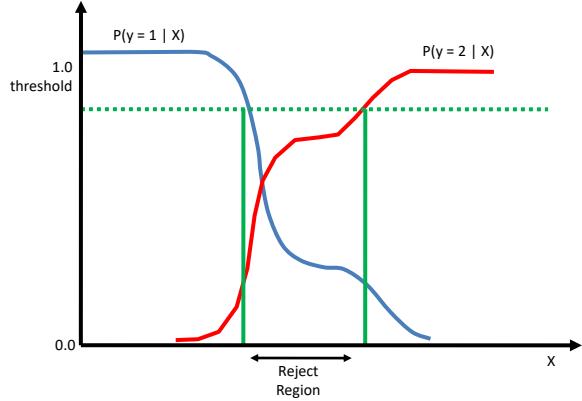
Figure 5.1: For some regions of input space, where the class posteriors are uncertain, we may prefer not to choose class 1 or 2; instead we may prefer the reject option. Adapted from Figure 1.26 of [Bis06].

		Estimate		Row sum
		0	1
	0	TN	FP	N
Truth	1	FN	TP	P
Col. sum		Nˆ	Pˆ

Table 5.3: Class confusion matrix for a binary classification problem. TP is the number of true positives, FP is the number of false positives, TN is the number of true negatives, FN is the number of false negatives, P is the true number of positives, Pˆ is the predicted number of positives, N is the true number of negatives, Nˆ is the predicted number of negatives.

which beat the top human Jeopardy champion. Watson uses a variety of interesting techniques [Fer+10], but the most pertinent one for our present discussion is that it contains a module that estimates how confident it is of its answer. The system only chooses to “buzz in” its answer if su”ciently confident it is correct.

For some other methods and applications, see e.g., [RTA18; GEY19; Nar+23].

5.1.3 ROC curves

In Section 5.1.2.2, we showed that we can pick the optimal label in a binary classification problem by thresholding the probability using a value τ , derived from the relative cost of a false positive and false negative. Instead of picking a single threshold, we can consider using a set of di!erent thresholds, and comparing the resulting performance, as we discuss below.

		Estimate
		0	1
Truth	0	TN/N=TNR=Spec	FP/N =FPR=Type I = Fallout
	1	FN/P=FNR=Miss=Type II	TP/P=TPR=Sens=Recall

Table 5.4: Class confusion matrix for a binary classification problem normalized per row to get p(yˆ|y). Abbreviations: TNR = true negative rate, Spec = specificity, FPR = false positive rate, FNR = false negative rate, Miss = miss rate, TPR = true positive rate, Sens = sensitivity. Note FNR=1-TPR and FPR=1-TNR.

\[\begin{array}{c|cc} & & \text{Estimate} & & \\ & 0 & 1 & \\ \hline \text{Truth} & 0 & \text{TN}/\hat{N}=\text{NPV} & \text{FP}/\hat{P}=\text{FDR} & \\ & 1 & \text{FN}/\hat{N}=\text{FOR} & \text{TP}/\hat{P}=\text{Prec}=\text{PPV} & \\ \end{array}\]

Table 5.5: Class confusion matrix for a binary classification problem normalized per column to get p(y|yˆ). Abbreviations: NPV = negative predictive value, FDR = false discovery rate, FOR = false omission rate, PPV = positive predictive value, Prec = precision. Note that FOR=1-NPV and FDR=1-PPV.

5.1.3.1 Class confusion matrices

For any fixed threshold τ , we consider the following decision rule:

\[\hat{y}\_{\tau}(\mathbf{z}) = \mathbb{I}\left(p(y=1|\mathbf{z}) \ge 1 - \tau\right) \tag{5.16}\]

We can compute the empirical number of false positives (FP) that arise from using this policy on a set of N labeled examples as follows:

\[FP\_{\tau} = \sum\_{n=1}^{N} \mathbb{I}\left(\hat{y}\_{\tau}(\mathbf{z}\_{n}) = 1, y\_{n} = 0\right) \tag{5.17}\]

Similarly, we can compute the empirical number of false negatives (FN), true positives (TP), and true negatives (TN). We can store these results in a 2 ↓ 2 class confusion matrix C, where Cij is the number of times an item with true class label i was (mis)classified as having label j. In the case of binary classification problems, the resulting matrix will look like Table 5.3.

From this table, we can compute p(yˆ|y) or p(y|yˆ), depending on whether we normalize across the rows or columns. We can derive various summary statistics from these distributions, as summarized in Table 5.4 and Table 5.5. For example, the true positive rate (TPR), also known as the sensitivity, recall or hit rate, is defined as

\[TPR\_{\tau} = p(\hat{y} = 1 | y = 1, \tau) = \frac{TP\_{\tau}}{TP\_{\tau} + FN\_{\tau}} \tag{5.18}\]

and the false positive rate (FPR), also called the false alarm rate, or the type I error rate, is defined as

\[FPR\_{\tau} = p(\hat{y} = 1 | y = 0, \tau) = \frac{FP\_{\tau}}{FP\_{\tau} + TN\_{\tau}} \tag{5.19}\]

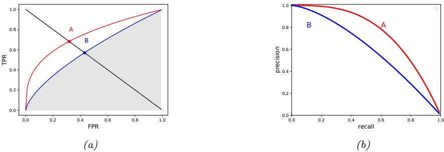
Figure 5.2: (a) ROC curves for two hypothetical classification systems. The red curve for system A is better than the blue curve for system B. We plot the true positive rate (TPR) vs the false positive rate (FPR) as we vary the threshold ▷ . We also indicate the equal error rate (EER) with the red and blue dots, and the area under the curve (AUC) for classifier B by the shaded area. Generated by roc\_plot.ipynb. (b) A precision-recall curve for two hypothetical classification systems. The red curve for system A is better than the blue curve for system B. Generated by pr\_plot.ipynb.

We can now plot the TPR vs FPR as an implicit function of τ . This is called a receiver operating characteristic or ROC curve. See Figure 5.2(a) for an example.

5.1.3.2 Summarizing ROC curves as a scalar

The quality of a ROC curve is often summarized as a single number using the area under the curve or AUC. Higher AUC scores are better; the maximum is obviously 1. Another summary statistic that is used is the equal error rate or EER, also called the cross-over rate, defined as the value which satisfies FPR = FNR. Since FNR=1-TPR, we can compute the EER by drawing a line from the top left to the bottom right and seeing where it intersects the ROC curve (see points A and B in Figure 5.2(a)). Lower EER scores are better; the minimum is obviously 0 (corresponding to the top left corner).

5.1.3.3 Class imbalance

In some problems, there is severe class imbalance. For example, in information retrieval, the set of negatives (irrelevant items) is usually much larger than the set of positives (relevant items). The ROC curve is una!ected by class imbalance, as the TPR and FPR are fractions within the positives and negatives, respectively. However, the usefulness of an ROC curve may be reduced in such cases, since a large change in the absolute number of false positives will not change the false positive rate very much, since FPR is divided by FP+TN (see e.g., [SR15] for discussion). Thus all the “action” happens in the extreme left part of the curve. In such cases, we may choose to use other ways of summarizing the class confusion matrix, such as precision-recall curves, which we discuss in Section 5.1.4.

5.1.4 Precision-recall curves

In some problems, the notion of a “negative” is not well-defined. For example, consider detecting objects in images: if the detector works by classifying patches, then the number of patches examined — and hence the number of true negatives — is a parameter of the algorithm, not part of the problem definition. Similarly, information retrieval systems usually get to choose the initial set of candidate items, which are then ranked for relevance; by specifying a cuto!, we can partition this into a positive and negative set, but note that the size of the negative set depends on the total number of items retrieved, which is an algorithm parameter, not part of the problem specification.

In these kinds of situations, we may choose to use a precision-recall curve to summarize the performance of our system, as we explain below. (See [DG06] for a more detailed discussion of the connection between ROC curves and PR curves.)

5.1.4.1 Computing precision and recall

The key idea is to replace the FPR with a quantity that is computed just from positives, namely the precision:

\[\mathcal{P}(\tau) \triangleq p(y=1|\hat{y}=1,\tau) = \frac{TP\_{\tau}}{TP\_{\tau} + FP\_{\tau}} \tag{5.20}\]

The precision measures what fraction of our detections are actually positive. We can compare this to the recall (which is the same as the TPR), which measures what fraction of the positives we actually detected:

\[\mathcal{R}(\tau) \triangleq p(\hat{y} = 1 | y = 1, \tau) = \frac{TP\_{\tau}}{TP\_{\tau} + FN\_{\tau}} \tag{5.21}\]

If yˆⁿ → {0, 1} is the predicted label, and yⁿ → {0, 1} is the true label, we can estimate precision and recall using

\[\mathcal{P}(\tau) = \frac{\sum\_{n} y\_n \hat{y}\_n}{\sum\_{n} \hat{y}\_n} \tag{5.22}\]

\[\mathcal{R}(\tau) = \frac{\sum\_{n}^{n \times \cdots} y\_n \hat{y}\_n}{\sum\_{n} y\_n} \tag{5.23}\]

We can now plot the precision vs recall as we vary the threshold τ . See Figure 5.2(b). Hugging the top right is the best one can do.

5.1.4.2 Summarizing PR curves as a scalar

The PR curve can be summarized as a single number in several ways. First, we can quote the precision for a fixed recall level, such as the precision of the first K = 10 entities recalled. This is called the precision at K score. Alternatively, we can compute the area under the PR curve. However, it is possible that the precision does not drop monotonically with recall. For example, suppose a classifier has 90% precision at 10% recall, and 96% precision at 20% recall. In this case, rather than measuring the precision at a recall of 10%, we should measure the maximum precision we can achieve with at least a recall of 10% (which would be 96%). This is called the interpolated

precision. The average of the interpolated precisions is called the average precision; it is equal to the area under the interpolated PR curve, but may not be equal to the area under the raw PR curve.1 The mean average precision or mAP is the mean of the AP over a set of di!erent PR curves.

5.1.4.3 F-scores

For a fixed threshold, corresponding to a single point on the PR curve, we can compute a single precision and recall value, which we will denote by P and R. These are often combined into a single statistic called the F⇀, defined as follows:2

\[\frac{1}{F\_{\beta}} = \frac{1}{1+\beta^2} \frac{1}{\mathcal{P}} + \frac{\beta^2}{1+\beta^2} \frac{1}{\mathcal{R}} \tag{5.24}\]

or equivalently

\[F\_{\beta} \triangleq (1+\beta^2) \frac{\mathcal{P} \cdot \mathcal{R}}{\beta^2 \mathcal{P} + \mathcal{R}} = \frac{(1+\beta^2)TP}{(1+\beta^2)TP + \beta^2 FN + FP} \tag{5.25}\]

If we set 1 = 1, we get the harmonic mean of precision and recall:

\[\frac{1}{F\_1} = \frac{1}{2} \left( \frac{1}{\mathcal{P}} + \frac{1}{\mathcal{R}} \right) \tag{5.26}\]

\[F\_1 = \frac{2}{1/\mathcal{R} + 1/\mathcal{P}} = 2\frac{\mathcal{P} \cdot \mathcal{R}}{\mathcal{P} + \mathcal{R}} = \frac{TP}{TP + \frac{1}{2}(FP + FN)}\tag{5.27}\]

To understand why we use the harmonic mean instead of the arithmetic mean, (P + R)/2, consider the following scenario. Suppose we recall all entries, so yˆⁿ = 1 for all n, and R = 1. In this case, the precision P will be given by the prevalence, p(y = 1) = ! ⁿ I(yn=1) ^N . Suppose the prevalence is low, say ^p(^y = 1) = 10→4. The arithmetic mean of ^P and ^R is given by (^{P + R})/2 = (10→⁴ + 1)/² ↖ 50%. By contrast, the harmonic mean of this strategy is only ²↔︎10↓4↔︎¹ 1+10↓⁴ ↖ 0.02%. In general, the harmonic mean is more conservative, and requires both precision and recall to be high.

Using F¹ score weights precision and recall equally. However, if recall is more important, we may use 1 = 2, and if precision is more important, we may use 1 = 0.5.

5.1.4.4 Class imbalance

ROC curves are insensitive to class imbalance, but PR curves are not, as noted in [Wil20]. To see this, let the fraction of positives in the dataset be ϑ = P/(P +N), and define the ratio r = P/N = ϑ/(1↑ϑ). Let n = P + N be the population size. ROC curves are not a!ected by changes in r, since the TPR is defined as a ratio within the positive examples, and FPR is defined as a ratio within the negative examples. This means it does not matter which class we define as positive, and which we define as negative.

Now consider PR curves. The precision can be written as

\[\text{Prec} = \frac{TP}{TP + FP} = \frac{P \cdot TPR}{P \cdot TPR + N \cdot FPR} = \frac{TPR}{TPR + \frac{1}{r}FPR} \tag{5.28}\]

^1. For details, see https://sanchom.wordpress.com/tag/average-precision/.

^2. We follow the notation from https://en.wikipedia.org/wiki/F-score#F%CE%B2.

Thus Prec ↔︎ 1 as ϑ ↔︎ 1 and r ↔︎ ∈, and Prec ↔︎ 0 as ϑ ↔︎ 0 and r ↔︎ 0. For example, if we change from a balanced problem where r = 0.5 to an imbalanced problem where r = 0.1 (so positives are rarer), the precision at each threshold will drop, and the recall (aka TPR) will stay the same, so the overall PR curve will be lower. Thus if we have multiple binary problems with di!erent prevalences (e.g., object detection of common or rare objects), we should be careful when averaging their precisions [HCD12].

The F-score is also a!ected by class imbalance. To see this, note that we can rewrite the F-score as follows:

\[\frac{1}{F\_{\beta}} = \frac{1}{1+\beta^2} \frac{1}{\mathcal{P}} + \frac{\beta^2}{1+\beta^2} \frac{1}{\mathcal{R}} \tag{5.29}\]

\[\frac{1}{1+\beta^2} \frac{TPR + \frac{N}{P}FPR}{TPR} + \frac{\beta^2}{1+\beta^2} \frac{1}{TPR} \tag{5.30}\]

\[F\_{\beta} = \frac{(1+\beta^2)TPR}{TPR + \frac{1}{r}FPR + \beta^2} \tag{5.31}\]

5.1.5 Regression problems

So far, we have considered the case where there are a finite number of actions A and states of nature H. In this section, we consider the case where the set of actions and states are both equal to the real line, A = H = R. We will specify various commonly used loss functions for this case (which can be extended to R^D by computing the loss elementwise.) The resulting decision rules can be used to compute the optimal parameters for an estimator to return, or the optimal action for a robot to take, etc.

5.1.5.1 L2 loss

The most common loss for continuous states and actions is the ω² loss, also called squared error or quadratic loss, which is defined as follows:

\[\ell\_2(h, a) = (h - a)^2 \tag{5.32}\]

In this case, the risk is given by

\[\rho(a|\mathbf{z}) = \mathbb{E}\left[ (h-a)^2 | \mathbf{z} \right] = \mathbb{E}\left[ h^2 | \mathbf{z} \right] - 2a\mathbb{E}\left[ h|\mathbf{z} \right] + a^2 \tag{5.33}\]

The optimal action must satisfy the condition that the derivative of the risk (at that point) is zero (as explained in Chapter 8). Hence the optimal action is to pick the posterior mean:

\[\frac{\partial}{\partial a}\rho(a|x) = -2\mathbb{E}\left[h|x\right] + 2a = 0 \implies \pi(x) = \mathbb{E}\left[h|x\right] = \int h \, p(h|x) dh\tag{5.34}\]

This is often called the minimum mean squared error estimate or MMSE estimate.

5.1.5.2 L1 loss

The ω² loss penalizes deviations from the truth quadratically, and thus is sensitive to outliers. A more robust alternative is the absolute or ω¹ loss

\[\ell\_1(h, a) = |h - a|\tag{5.35}\]

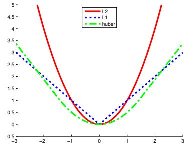
Figure 5.3: Illustration of ,2, ,1, and Huber loss functions with ◁ = 1.5. Generated by huberLossPlot.ipynb.

This is sketched in Figure 5.3. Exercise 5.4 asks you to show that the optimal estimate is the posterior median, i.e., a value a such that Pr(h<a|x) = Pr(h ∋ a|x)=0.5. We can use this for robust regression as discussed in Section 11.6.1.

5.1.5.3 Huber loss

Another robust loss function is the Huber loss [Hub64], defined as follows:

\[\ell\_{\delta}(h, a) = \begin{cases} |r^2/2 & \text{if } |r| \le \delta \\ \delta |r| - \delta^2/2 & \text{if } |r| > \delta \end{cases} \tag{5.36}\]

where r = h ↑ a. This is equivalent to ω² for errors that are smaller than ↽, and is equivalent to ω¹ for larger errors. See Figure 5.3 for a plot. We can use this for robust regression as discussed in Section 11.6.3.

5.1.6 Probabilistic prediction problems

In Section 5.1.2, we assumed the set of possible actions was to pick a single class label (or possibly the “reject” or “do not know” action). In Section 5.1.5, we assumed the set of possible actions was to pick a real valued scalar. In this section, we assume the set of possible actions is to pick a probability distribution over some value of interest. That is, we want to perform probabilistic prediction or probabilistic forecasting, rather than predicting a specific value. More precisely, we assume the true “state of nature” is a distribution, h = p(Y |x), the action is another distribution, a = q(Y |x), and we want to pick q to minimize E [ω(p, q)] for each given x. We discuss various possible loss functions below. We drop the conditioning on x for brevity.

5.1.6.1 KL, cross-entropy and log-loss

A common form of loss functions for comparing two distributions is the Kullback Leibler divergence, or KL divergence, which is defined as follows:

\[D\_{\mathbb{KL}}\left(p \parallel q\right) \triangleq \sum\_{y \in \mathcal{Y}} p(y) \log \frac{p(y)}{q(y)}\tag{5.37}\]

(We have assumed the variable y is discrete, for notational simplicity, but this can be generalized to real-valued variables.) In Section 6.2, we show that the KL divergence satisfies the following properties: DKL (p 7 q) ∋ 0 with equality i! p = q. Note that it is an asymmetric function of its arguments.

We can expand the KL as follows:

\[D\_{\mathbb{KL}}\left(p \parallel q\right) = \sum\_{y \in \mathcal{Y}} p(y) \log p(y) - \sum\_{y \in \mathcal{Y}} p(y) \log q(y) \tag{5.38}\]

\[=-\mathbb{H}(p) + \mathbb{H}\_{ce}(p, q) \tag{5.39}\]

\[\mathbb{H}(p) \stackrel{\Delta}{=} -\sum\_{y} p(y) \log p(y) \tag{5.40}\]

\[\mathbb{H}\_{cc}(p,q) \stackrel{\Delta}{=} -\sum\_{y} p(y)\log q(y) \tag{5.41}\]

The H(p) term is known as the entropy. This is a measure of uncertainty or variance of p; it is maximal if p is uniform, and is 0 if p is a degenerate or deterministic delta function. Entropy is often used in the field of information theory, which is concerned with optimal ways of compressing and communicating data (see Chapter 6). The optimal coding scheme will allocate fewer bits to more frequent symbols (i.e., values of Y for which p(y) is large), and more bits to less frequent symbols. A key result states that the number of bits needed to compress a dataset generated by a distribution p is at least H(p); the entropy therefore provides a lower bound on the degree to which we can compress data without losing information. The Hce(p, q) term is known as the cross-entropy. This measures the expected number of bits we need to use to compress a dataset coming from distribution p if we design our code using distribution q. Thus the KL is the extra number of bits we need to use to compress the data due to using the incorrect distribution q. If the KL is zero, it means that we can correctly predict the probabilities of all possible future events, and thus we have learned to predict the future as well as an “oracle” that has access to the true distribution p.

To find the optimal distribution to use when predicting future data, we can minimize DKL (p 7 q). Since H(p) is a constant wrt q, it can be ignored, and thus we can equivalently minimize the cross-entropy:

\[q^\*(Y) = \operatorname\*{argmin}\_q \mathbb{H}\_{ce}(p(Y), q(Y))\tag{5.42}\]

Now consider the special case in which the true state of nature is a degenerate distribution, which puts all its mass on a single outcome, say c, i.e., h = p(Y ) = I(Y = c). This is often called a “one-hot” distribution, since it turns “on” the c’th element of the vector, and leaves the other elements “o!”, as shown in Figure 2.1. In this case, the cross entropy becomes

\[\mathbb{H}\_{cc}(\delta(Y=c),q) = -\sum\_{y \in \mathcal{Y}} \delta(y=c) \log q(y) = -\log q(c) \tag{5.43}\]

This is known as the log loss of the predictive distribution q when given target label c.

5.1.6.2 Proper scoring rules

Cross-entropy loss is a very common choice for probabilistic forecasting, but is not the only possible metric. The key property we desire is that the loss function is minimized i! the decision maker picks

the distribution q that matches the true distribution p, i.e., ω(p, p) ↘ ω(p, q), with equality i! p = q. Such a loss function ω is called a proper scoring rule [GR07]. We can show that cross-entropy loss is a proper scoring rule by virtue of the fact that 0 = DKL (p 7 p) ↘ DKL (p 7 q).

5.1.6.3 Brier score

The log[p(y)/q(y)] term in the KL loss can be quite sensitive to errors for low probability events [QC+06]. A common alternative is to use the Brier score [Bri50], which is another proper scoring rule, originally invented in the context of weather forecasting. This is defined for the special case that the true distribution p is a set of N delta functions, pn(Yn) = ↽(Yⁿ ↑ yn), where yⁿ is the observed outcome in one-hot form, so ync = 1 if the n’th observed outcome is class c. The corresponding predictive distribution is assumed to be a set of N distributions qn(Yn), which can of course be conditioned on covariates xn. The Brier score can now be defined as follows:

\[\text{BS}(\mathbf{p}, \mathbf{q}) \triangleq \frac{1}{N} \sum\_{n=1}^{N} \sum\_{c=1}^{C} (q\_{nc} - p\_{nc})^2 = \frac{1}{N} \sum\_{n=1}^{N} \sum\_{c=1}^{C} (q\_{nc} - y\_{nc})^2 \tag{5.44}\]

This is just the mean squared error of the predictive distributions compared to the true distributions, when viewed as vectors. Since it is based on squared error, the Brier score is less sensitive to extremely rare or extremely common classes.

In the special case of binary classification, where we use class labels c = 0 and c = 1, we define ^{yn = y}n1, and ^{qn = q}(Yn1), so the summand becomes (q^{n ↑ y}n)² + (1 ^{↑ qn ↑} (1 ^{↑ y}n))² = 2(q^{n ↑ y}n)2. Consequently, in the binary cases, we often divide the multi-class definition by 2, to get the binary Brier Score, BS(p, q) = ¹ N $^{N n}=1(q^{n ↑ y}n)², which has values in the range [0, 1], with the optimal loss being 0.

Since it can be hard to interpret absolute Brier score values, a relative performance measure, known as the Brier Skill Score, is sometimes used. This is defined as BSS = 1 ^↑ BS BSref , where BSref is the BS of a reference model. The range of this score is [↑1, 1], with 1 being the best, 0 meaning no improvement over the baseline. and -1 being the worst. In the case of binary predictors, a common reference model is the baseline empirical probability q = ¹ N $^{N n}=1 yn. In the metereological community, this is called the “in-sample climatology” prediction, where “in-sample” means based on the observed data, and “climatology” refers to the long run average behavior. However, the reference model could be a sophisticated numerical weather prediction model, and the target model (which is being evaluated) could be an ML model (see e.g., [Pri+23]).

5.2 Choosing the “right” model

In this section, we consider the setting in which we have several candidate (parametric) models (e.g., neural networks with di!erent numbers of layers), and we want to choose the “right” one. This can be tackled using tools from Bayesian decision theory.

5.2.1 Bayesian hypothesis testing

Suppose we have two hypotheses or models, commonly called the null hypothesis, M0, and the alternative hypothesis, M1, and we want to know which one is more likely to be true. This is called hypothesis testing.

Bayes factor BF(1, 0)	Interpretation
1 BF < 100	Decisive evidence for M0
1 BF < 10	Strong evidence for M0
1 1 10 < BF < 3	M0 Moderate evidence for
1 3 < BF < 1	Weak evidence for M0
1 < BF < 3	Weak evidence for M1
3 < BF < 10	Moderate evidence for M1
BF > 10	Strong evidence for M1
BF > 100	Decisive evidence for M1

Table 5.6: Je!reys scale of evidence for interpreting Bayes factors.

If we use 0-1 loss, the optimal decision is to pick the alternative hypothesis i! p(M1|D) > p(M0|D), or equivalently, if p(M1|D)/p(M0|D) > 1. If we use a uniform prior, p(M0) = p(M1)=0.5, the decision rule becomes: select M¹ i! p(D|M1)/p(D|M0) > 1. This quantity, which is the ratio of marginal likelihoods of the two models, is known as the Bayes factor:

\[B\_{1,0} \stackrel{\Delta}{=} \frac{p(\mathcal{D}|M\_1)}{p(\mathcal{D}|M\_0)}\tag{5.45}\]

This is like a likelihood ratio, except we integrate out the parameters, which allows us to compare models of di!erent complexity, due to the Bayesian Occam’s razor e!ect explained in Section 5.2.3.

If B1,⁰ > 1 then we prefer model 1, otherwise we prefer model 0. Of course, it might be that B1,⁰ is only slightly greater than 1. In that case, we are not very confident that model 1 is better. Je!reys [Jef61] proposed a scale of evidence for interpreting the magnitude of a Bayes factor, which is shown in Table 5.6. This is a Bayesian alternative to the frequentist concept of a p-value (see Section 5.5.3).

We give a worked example of how to compute Bayes factors in Section 5.2.1.1.

5.2.1.1 Example: Testing if a coin is fair

As an example, suppose we observe some coin tosses, and want to decide if the data was generated by a fair coin, ϖ = 0.5, or a potentially biased coin, where ϖ could be any value in [0, 1]. Let us denote the first model by M⁰ and the second model by M1. The marginal likelihood under M⁰ is simply

\[p(\mathcal{D}|M\_0) = \left(\frac{1}{2}\right)^N\tag{5.46}\]

where N is the number of coin tosses. From Equation (4.143), the marginal likelihood under M1, using a Beta prior, is

\[p(\mathcal{D}|M\_1) = \int p(\mathcal{D}|\theta)p(\theta)d\theta = \frac{B(\alpha\_1 + N\_1, \alpha\_0 + N\_0)}{B(\alpha\_1, \alpha\_0)}\tag{5.47}\]

We plot log p(D|M1) vs the number of heads N¹ in Figure 5.4(a), assuming N = 5 and a uniform prior, ϱ¹ = ϱ⁰ = 1. (The shape of the curve is not very sensitive to ϱ¹ and ϱ0, as long as the prior is symmetric, so ϱ⁰ = ϱ1.) If we observe 2 or 3 heads, the unbiased coin hypothesis M⁰

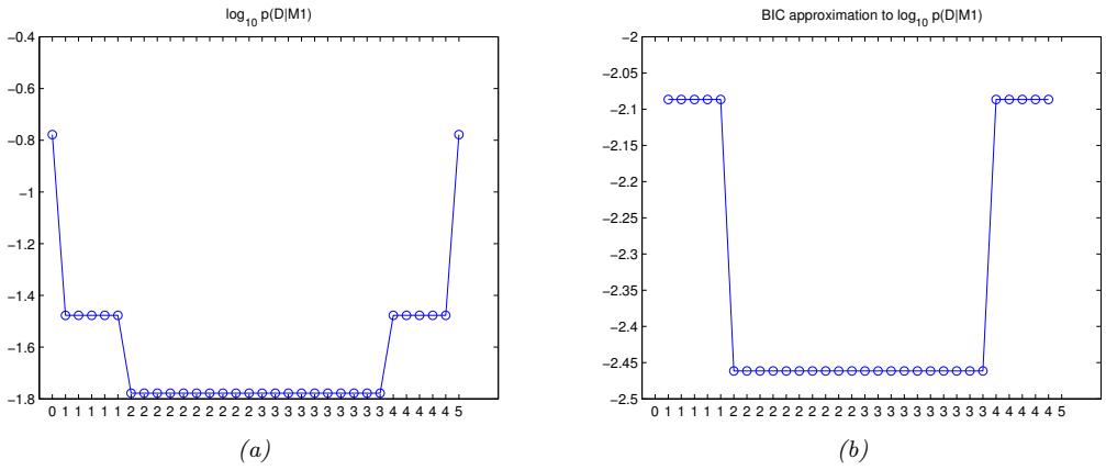
Figure 5.4: (a) Log marginal likelihood vs number of heads for the coin tossing example. (b) BIC approximation. (The vertical scale is arbitrary, since we are holding N fixed.) Generated by coins\_model\_sel\_demo.ipynb.

is more likely than M1, since M⁰ is a simpler model (it has no free parameters) — it would be a suspicious coincidence if the coin were biased but happened to produce almost exactly 50/50 heads/tails. However, as the counts become more extreme, we favor the biased coin hypothesis. Note that, if we plot the log Bayes factor, log B1,0, it will have exactly the same shape, since log p(D|M0) is a constant.

5.2.2 Bayesian model selection

Now suppose we have a set M of more than 2 models, and we want to pick the most likely. This is called model selection. We can view this as a decision theory problem, where the action space requires choosing one model, m → M. If we have a 0-1 loss, the optimal action is to pick the most probable model:

\[ \hat{m} = \underset{m \in \mathcal{M}}{\text{argmax}} \, p(m|\mathcal{D}) \tag{5.48} \]

where

\[p(m|\mathcal{D}) = \frac{p(\mathcal{D}|m)p(m)}{\sum\_{m \in \mathcal{M}} p(\mathcal{D}|m)p(m)}\tag{5.49}\]

is the posterior over models. If the prior over models is uniform, p(m)=1/|M|, then the MAP model is given by

\[ \hat{m} = \underset{m \in \mathcal{M}}{\text{argmax}} \, p(\mathcal{D}|m) \tag{5.50} \]

The quantity p(D|m) is given by

\[p(\mathcal{D}|m) = \int p(\mathcal{D}|\theta, m)p(\theta|m)d\theta\tag{5.51}\]

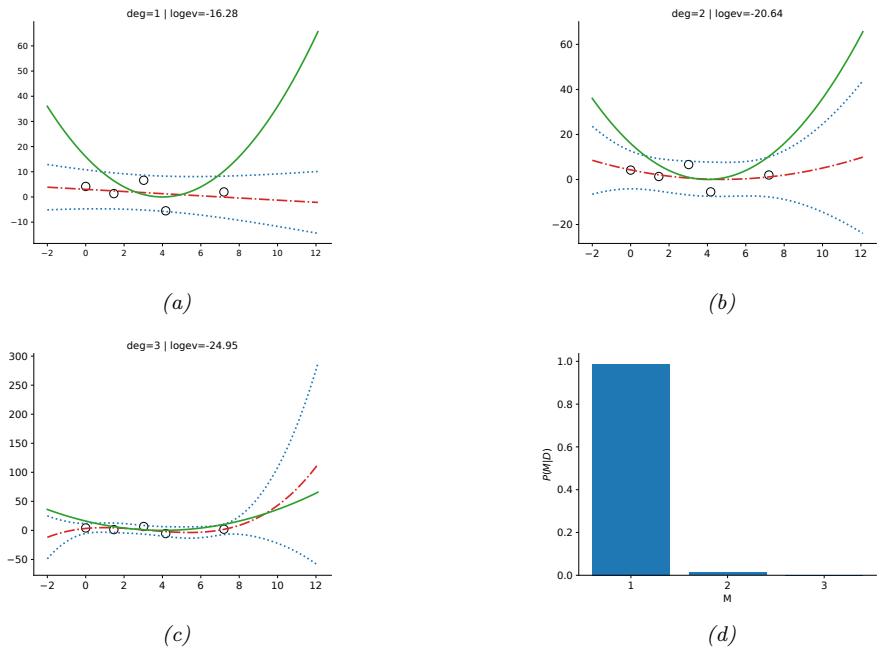
Figure 5.5: Ilustration of Bayesian model selection for polynomial regression. (a-c) We fit polynomials of degrees 1, 2 and 3 fit to N = 5 data points. The solid green curve is the true function, the dashed red curve is the prediction (dotted blue lines represent ±2ϑ around the mean). (d) We plot the posterior over models, p(m|D), assuming a uniform prior p(m) ∝ 1. Generated by linreg\_eb\_modelsel\_vs\_n.ipynb.

This is known as the marginal likelihood, or the evidence for model m. Intuitively, it is the likelihood of the data averaged over all possible parameter values, weighted by the prior p(ω|m). If all settings of ω assign high probability to the data, then this is probably a good model.

5.2.2.1 Example: polynomial regression

As an example of Bayesian model selection, we will consider polynomial regression in 1d. Figure 5.5 shows the posterior over three di!erent models, corresponding to polynomials of degrees 1, 2 and 3 fit to N = 5 data points. We use a uniform prior over models, and use empirical Bayes to estimate the prior over the regression weights (see Section 11.7.7). We then compute the evidence for each model (see Section 11.7 for details on how to do this). We see that there is not enough data to justify a complex model, so the MAP model is m = 1. Figure 5.6 shows the analogous plot for N = 30 data points. Now we see that the MAP model is m = 2; the larger sample size means we can safely pick a more complex model.

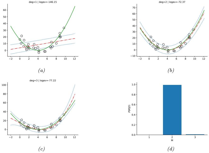
Figure 5.6: Same as Figure 5.5 except now N = 30. Generated by linreg\_eb\_modelsel\_vs\_n.ipynb.

5.2.3 Occam’s razor

Consider two models, a simple one, m1, and a more complex one, m2. Suppose that both can explain the data by suitably optimizing their parameters, i.e., for which ^p(D|ωˆ1, m1) and ^p(D|ωˆ2, m2) are both large. Intuitively we should prefer m1, since it is simpler and just as good as m2. This principle is known as Occam’s razor.

Let us now see how ranking models based on their marginal likelihood, which involves averaging the likelihood wrt the prior, will give rise to this behavior. The complex model will put less prior probability on the “good” parameters that explain the data, ωˆ2, since the prior must integrate to 1.0 over the entire parameter space. Thus it will take averages in parts of parameter space with low likelihood. By contrast, the simpler model has fewer parameters, so the prior is concentrated over a smaller volume; thus its averages will mostly be in the good part of parameter space, near ωˆ1. Hence we see that the marginal likelihood will prefer the simpler model. This is called the Bayesian Occam’s razor e!ect [Mac95; MG05].

Another way to understand the Bayesian Occam’s razor e!ect is to compare the relative predictive abilities of simple and complex models. Since probabilities must sum to one, we have $ ^{D→ p}(D↗ |m)=1, where the sum is over all possible datasets. Complex models, which can predict many things, must spread their predicted probability mass thinly, and hence will not obtain as large a probability for any given data set as simpler models. This is sometimes called the conservation of probability mass principle, and is illustrated in Figure 5.7. On the horizontal axis we plot all possible data sets in order of increasing complexity (measured in some abstract sense). On the vertical axis we plot the

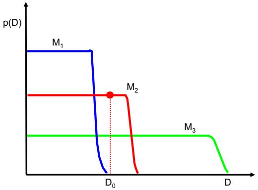
Figure 5.7: A schematic illustration of the Bayesian Occam’s razor. The broad (green) curve corresponds to a complex model, the narrow (blue) curve to a simple model, and the middle (red) curve is just right. Adapted from Figure 3.13 of [Bis06]. See also [MG05, Figure 2] for a similar plot produced on real data.

predictions of 3 possible models: a simple one, M1; a medium one, M2; and a complex one, M3. We also indicate the actually observed data D⁰ by a vertical line. Model 1 is too simple and assigns low probability to D0. Model 3 also assigns D⁰ relatively low probability, because it can predict many data sets, and hence it spreads its probability quite widely and thinly. Model 2 is “just right”: it predicts the observed data with a reasonable degree of confidence, but does not predict too many other things. Hence model 2 is the most probable model.

5.2.4 Connection between cross validation and marginal likelihood

We have seen how the marginal likelihood helps us choose models of the “right” complexity. In non-Bayesian approaches to model selection, it is standard to use cross validation (Section 4.5.5) for this purpose.

It turns out that the marginal likelihood is closely related to the leave-one-out cross-validation (LOO-CV) estimate, as we now show. We start with the marginal likelihood for model m, which we write in sequential form as follows:

\[p(\mathcal{D}|m) = \prod\_{n=1}^{N} p(y\_n|y\_{1:n-1}, x\_{1:N}, m) = \prod\_{n=1}^{N} p(y\_n|x\_n, \mathcal{D}\_{1:n-1}, m) \tag{5.52}\]

where

\[p(y|\mathbf{z}, \mathcal{D}\_{1:n-1}, m) = \int p(y|\mathbf{z}, \theta) p(\theta|\mathcal{D}\_{1:n-1}, m) d\theta \tag{5.53}\]

Suppose we use a plugin approximation to the above distribution to get

\[p(y|x,\mathcal{D}\_{1:n-1},m) \approx \int p(y|x,\boldsymbol{\theta})\delta(\boldsymbol{\theta}-\hat{\boldsymbol{\theta}}\_{m}(\mathcal{D}\_{1:n-1}))d\boldsymbol{\theta} = p(y|x,\hat{\boldsymbol{\theta}}\_{m}(\mathcal{D}\_{1:n-1}))\tag{5.54}\]

Then we get

\[\log p(\mathcal{D}|m) \approx \sum\_{n=1}^{N} \log p(y\_n|x\_n, \hat{\theta}\_m(\mathcal{D}\_{1:n-1})) \tag{5.55}\]

This is similar to a leave-one-out cross-validation estimate of the likelihood, which has the form 1 N $^{N n}=1 log ^p(yn|xn, ^ωˆm(D1:n→1,n+1:^N )), except we ignore the ^Dn+1:^N part. The intuition behind the connection is this: an overly complex model will overfit the “early” examples and will then predict the remaining ones poorly, and thus will also get a low cross-validation score. See [FH20] for a more detailed discussion of the connection between these performance metrics.

5.2.5 Information criteria

The marginal likelihood, ^p(D|m) = ^{H p}(D|ω, m)p(ω)dω, which is needed for Bayesian model selection discussed in Section 5.2.2, can be di”cult to compute, since it requires marginalizing over the entire parameter space. Furthermore, the result can be quite sensitive to the choice of prior. In this section, we discuss some other related metrics for model selection known as information criteria. These have the following form: ^L(m) = ^↑ log ^p(D|ωˆ, m) + ^C(m), where ^C(m) is a complexity penalty term added to the negative log likelihood (NLL). Di!erent methods use di!erent complexity terms C(m), as we discuss below. See e.g., [GHV14] for further details.

A note on notation: it is conventional, when working with information criteria, to scale the NLL by ^↑2 to get the deviance, deviance(m) = ^↑2 log ^p(D|ωˆ, m). This makes the math “prettier” for certain Gaussian models.

5.2.5.1 The Bayesian information criterion (BIC)

The Bayesian information criterion or BIC [Sch78] can be thought of as a simple approximation to the log marginal likelihood. In particular, if we make a Gaussian approximation to the posterior, as discussed in Section 4.6.8.2, we get (from Equation (4.215)) the following:

\[\log p(\mathcal{D}|m) \approx \log p(\mathcal{D}|\hat{\theta}\_{\text{map}}) + \log p(\hat{\theta}\_{\text{map}}) - \frac{1}{2} \log |\mathbf{H}| \tag{5.56}\]

where ^H is the Hessian of the negative log joint, ^↑ log ^p(D, ^ω), evaluated at the MAP estimate ^ωˆmap. We see that Equation (5.56) is the log likelihood plus some penalty terms. If we have a uniform prior, ^p(ω) ^{∞ 1}, we can drop the prior term, and replace the MAP estimate with the MLE, ^ωˆ, yielding

\[\log p(\mathcal{D}|m) \approx \log p(\mathcal{D}|\hat{\theta}) - \frac{1}{2}\log|\mathbf{H}|\tag{5.57}\]

We now focus on approximating the log |H| term, which is sometimes called the Occam factor, since it is a measure of model complexity (volume of the posterior distribution). We have H = $^{N i}=1 Hi, where Hⁱ = ̸̸ log p(yi|ω) is the empirical Fisher information matrix (Section 4.7.2). Let us approximate each Hⁱ by a fixed matrix Hˆ . Then we have

\[\log|\mathbf{H}| = \log|N\hat{\mathbf{H}}| = \log(N^{D\_m}|\hat{\mathbf{H}}|) = D\_m \log N + \log|\hat{\mathbf{H}}|\tag{5.58}\]

where ^{Dm =} dim(ω) and we have assumed ^H is full rank. We can drop the log ^|H^{ˆ |} term, since it is independent of N, and thus will get overwhelmed by the likelihood. Putting all the pieces together, we get the BIC score that we want to maximize:

\[J\_{\rm BIC}(m) = \log p(\mathcal{D}|m) \approx \log p(\mathcal{D}|\hat{\theta}, m) - \frac{D\_m}{2} \log N \tag{5.59}\]

We can also define the BIC loss, that we want to minimize, by multiplying by -2:

\[\mathcal{L}\_{\text{BIC}}(m) = -2\log p(\mathcal{D}|\hat{\theta}, m) + D\_m \log N\tag{5.60}\]

(The use of 2 as a scale factor is chosen to simplify the expression when using a model with a Gaussian likelihood.)

5.2.5.2 Akaike information criterion

The Akaike information criterion [Aka74] is closely related to the BIC. It has the form

\[\mathcal{L}\_{\text{AIC}}(m) = -2\log p(\mathcal{D}|\hat{\theta}, m) + 2D\_m \tag{5.61}\]

This penalizes complex models less heavily than BIC, since the regularization term is independent of N. This estimator can be derived from a frequentist perspective.

5.2.5.3 Minimum description length (MDL)

We can think about the problem of scoring di!erent models by using tools from information theory (Chapter 6). In particular, suppose we want to choose a model so that the sender can send some dataa to the receiver using the fewest number of bits. Choosing models this way is known as the minimum description length or MDL principle (see e.g., [HY01b; Gru07; GR19] for details, and see [Wal05] for the closely related minimum message length criterion).

We now derive an approximation to the MDL objective. First, the sender needs to specify which model to use. Let ^{ωˆ → RDm} be the parameters estimated using ^N data samples. Since we can only reliably estimate each parameter to an accuracy of O(1/ ≃ N) (see Section 4.6.4.1), we only need to use log2(1/ ≃ N) = ^{1 2} log2(N) bits to encode each parameter. Second, the sender needs to use this model to encode the data, which takes ^↑ log ^p(D|ωˆ, m) = ^↑$ ⁿ log ^p(yn|ωˆ, m) bits. The total cost is

\[\mathcal{L}\_{\text{MDL}}(m) = -\log p(\mathcal{D}|\hat{\theta}, m) + \frac{D\_m}{2} \log N \tag{5.62}\]

We see that this two-part code has the same basic form as BIC.

5.2.5.4 Widely applicable information criterion (WAIC)

The main problem with BIC, AIC and MDL is that it can be hard to compute the degrees of a freedom of a model, needed to define the complexity term, since most parameters are highly correlated and not uniquely identifiable from the likelihood. In particular, if the mapping from parameters to the likelihood is not one-to-one, then the model known as a singular statistical model, since the corresponding Fisher information matrix (Section 4.7.2), and hence the Hessian H above, may be

singular. (Similar problems arise in over-parameterized models [Dwi+23].) An alternative criterion that works even in the singular case is known as the widely applicable information criterion (WAIC), also known as the Watanabe–Akaike information criterion [Wat10; Wat13].

The WAIC replaces the plug-in approximation to the marginal log likelihood, ω(m) = $ ⁿ log ^p(yn|ωˆ, m) with the the expected log pointwise predictive density or ELPD, defined as ELPD(m) = $^{N n}=1 log ^p(yn|D, m) = $^{N n}=1 log Eω|D,m[p(yn|ω, m)], which is usually approximated by Monte Carlo. In addition, the complexity term is defined by C(m) = $^{N n}=1 log V^ω|D,m[p(yn|ω, m)], which again is usually approximated by Monte Carlo. (The intuition for this is as follows: if, for a given datapoint yn, the di!erent posterior samples ω^s make very di!erent predictions, then the model is uncertain, and likely too flexible. The complexity term essentially counts how often this occurs.) The WAIC loss we want to minimize is defined as LWAIC(m) = ↑2LPPD(m)+2C(m).

Note that the WAIC evaluates the expected log likelihood using the posterior of the parameters. By contrast, the marginal likelihood averages the log likelihood wrt the prior. This makes the ML more sensitive to the prior. It is therefore generally better to use WAIC for model selection. E”cient Monte Carlo appproximations are discussed in [VGG17].

5.2.6 Posterior inference over e!ect sizes and Bayesian significance testing

The approach to hypothesis testing discussed in Section 5.2.1 relies on computing the Bayes factors for the null vs the alternative model, p(D|H0)/p(D|H1). Unfortunately, computing the necessary marginal likelihoods can be computationally di”cult, and the results can be sensitive to the choice of prior. Furthermore, we are often more interested in estimating an e”ect size, which is the di!erence in magnitude between two parameters, rather than in deciding if an e!ect size is 0 (null hypothesis) or not (alternative hypothesis) — the latter is called a point null hypothesis, and is often regarded as an irrelevant “straw man” (see e.g., [Mak+19] and references therein).

For example, suppose we have two classifiers, m¹ and m2, and we want to know which one is better. That is, we want to perform a comparison of classifiers. Let µ¹ and µ² be their average accuracies, and let % = µ¹ ↑ µ² be the di!erence in their accuracies. The probability that model 1 is more accurate, on average, than model 2 is given by p(% > 0|D). However, even if this probability is large, the improvement may be not be practically significant. So it is better to compute a probability such as p(% > ▷|D) or p(|%| > ▷|D), where ▷ represents the minimal magnitude of e!ect size that is meaningful for the problem at hand. This is called a one-sided test or two-sided test.

More generally, let R = [↑▷, ▷] represent a region of practical equivalence or ROPE [Kru15; KL17]. We can define 3 events of interest: the null hypothesis H⁰ : % → R, which says both methods are practically the same (which is a more realistic assumption than H⁰ : % = 0); H^A : % > ▷, which says m¹ is better than m2; and H^B : % < ↑▷, which says m² is better than m1. To choose amongst these 3 hypotheses, we just have to compute p(%|D), which avoids the need to compute Bayes factors. In the sections below, we discuss how to compute this quantity using two di!erent kinds of model.

5.2.6.1 Bayesian t-test for di”erence in means

Suppose we have two classifiers, m¹ and m2, which are evaluated on the same set of N test examples. Let e^{m i} be the error of method m on test example i. (Or this could be the conditional log likelihood, e^{m i =} log ^pm(yi|xi).) Since the classifiers are applied to the same data, we can use a paired test for comparing them, which is more sensitive than looking at average performance, since the factors that

make one example easy or hard to classify (e.g., due to label noise) will be shared by both methods. Thus we will work with the di!erences, dⁱ = e^{1 i ↑ e2 i} . We assume ^{di ⇒ N} (%, ^ε2). We are interested in p(%|d), where d = (d1,…,d^N ).

If we use an uninformative prior for the unknown parameters (%, ε), one can show that the posterior marginal for the mean is given by a Student distribution:

\[p(\Delta|\mathbf{d}) = \mathcal{T}\_{N-1}(\Delta|\mu, s^2/N)\]

where µ = ¹ N $^{N i}=1 dⁱ is the sample mean, and s² = ¹ N→1 $^{N i}=1(d^{i ↑ µ})² is an unbiased estimate of the variance. Hence we can easily compute p(|%| > ▷|d), with a ROPE of ▷ = 0.01 (say). This is known as a Bayesian t-test [Ben+17]. (See also [Rou+09] for Bayesian t-test based on Bayes factors, and [Die98] for a non-Bayesian approach to comparing classifiers.)

An alternative to a formal test is to just plot the posterior p(%|d). If this distribution is tightly centered on 0, we can conclude that there is no significant di!erence between the methods. (In fact, an even simpler approach is to just make a boxplot of the data, {di}, which avoids the need for any formal statistical analysis.)

Note that this kind of problem arises in many applications, not just evaluating classifiers. For example, suppose we have a set of N people, each of whom is exposed two drugs; let e^{m i} be the outcome (e.g., sickness level) when person i is exposed to drug m, and let d^{m i} = e^{1 i ↑ e2 i} be the di!erence in response. We can then analyse the e!ect of the drug by computing p(%|d) as we discussed above.

5.2.6.2 Bayesian ↽²-test for di”erence in rates

Now suppose we have two classifiers which are evaluated on di!erent test sets. Let y^m be the number of correct examples from method m → {1, 2} out of N^m trials, so the accuracy rate is ym/Nm. We assume y^m ⇒ Bin(Nm, ϖm), so we are interested in p(%|D), where % = ϖ¹ ↑ ϖ2, and D = (y1, N1, y2, N2) is all the data.

If we use a uniform prior for ϖ¹ and ϖ² (i.e., p(ϖ^j ) = Beta(ϖ^j |1, 1)), the posterior is given by

\[p(\theta\_1, \theta\_2 | \mathcal{D}) = \text{Beta}(\theta\_1 | y\_1 + 1, N\_1 - y\_1 + 1) \text{Beta}(\theta\_2 | y\_2 + 1, N\_2 - y\_2 + 1)\]

The posterior for % is given by

\[\begin{aligned} p(\Delta|\mathcal{D}) &= \int\_0^1 \int\_0^1 \mathbb{I}\left(\Delta = \theta\_1 - \theta\_2\right) p(\theta\_1|\mathcal{D}\_1) p(\theta\_2|\mathcal{D}\_2) \\ &= \int\_0^1 \text{Beta}(\theta\_1|y\_1 + 1, N\_1 - y\_1 + 1) \text{Beta}(\theta\_1 - \Delta|y\_2 + 1, N\_2 - y\_2 + 1) d\theta\_1 \end{aligned}\]

We can then evaluate this for any value of % that we choose. For example, we can compute

\[p(\Delta > \epsilon | \mathcal{D}) = \int\_{\epsilon}^{\infty} p(\Delta | \mathcal{D}) d\Delta \tag{5.63}\]

(We can compute this using 1 dimensional numerical integration or analytically [Coo05].) This is called a Bayesian χ²-test.

	LH	RH
Male	9	43	N1 = 52
Female	4	44	N2 = 48
Totals	13	87	100

Table 5.7: A 2 → 2 contingency table from http: // en. wikipedia. org/ wiki/ Contingency\_ table . The MLEs for the left handedness rate in males and females are ˆε¹ = 9/52 = 0.1731 and ˆε² = 4/48 = 0.0417.

Note that this kind of problem arises in many applications, not just evaluating classifiers, For example, suppose the two groups are di!erent companies selling the same product on Amazon, and y^m is the number of positive reviews for merchant m. Or suppose the two groups correspond to men and women, and y^m is the number of people in group m who are left handed, and N^m ↑ y^m to be the number who are right handed.3 We can represent the data as a 2 ^↓ 2 contingency table of counts, as shown in Table 5.7.

The MLEs for the left handedness rate in males and females are ˆϖ¹ = 9/52 = 0.1731 and ˆϖ² = 4/48 = 0.0417. It seems that there is a di!erence, but the sample size is low, so we cannot be sure. Hence we will represent our uncertainty by computing p(%|D), where % = ϖ¹ ↑ ϖ² and D is the table of counts. We find ^p(ϖ^{1 &}gt; ^ϖ2|D) = ^H ↘ ⁰ p(%|D)=0.901, which suggests that left handedness is more common in males, consistent with other studies [PP+20].

5.3 Frequentist decision theory

In this section, we discuss frequentist decision theory. In this approach, we treat the unknown state of nature (often denoted by ω instead of h) as a fixed but unknown quantity, and we treat the data x as random. Thus instead of conditioning on x, we average over it, to compute the loss we expect to incur if we apply our decision procedure (estimator) to many di!erent datasets. We give the details below.

5.3.1 Computing the risk of an estimator

We define the frequentist risk of an estimator ↽ given an unknown state of nature ω to be the expected loss when applying that estimator to data x, where the expectation is over the data, sampled from p(x|ω):

\[R(\theta,\delta) \stackrel{\Delta}{=} \mathbb{E}\_{p(\mathbf{z}|\theta)} \left[ \ell(\theta,\delta(\mathbf{z})) \right] \tag{5.64}\]

We give an example of this in Section 5.3.1.1.

5.3.1.1 Example

In this section, we consider the problem of estimating the mean of a Gaussian. We assume the data is sampled from ^{xn ⇒ N} (ϖ↓, ^ε2 = 1), and we let ^x = (x1,…,x^N ). If we use quadratic loss, ^ω2(ϖ, ^ˆϖ)=(^{ϖ ↑ ˆ}ϖ)², the corresponding risk function is the MSE.

^3. This example is based on the following blog post by Bob Carpenter: https://bit.ly/2FykD1C.

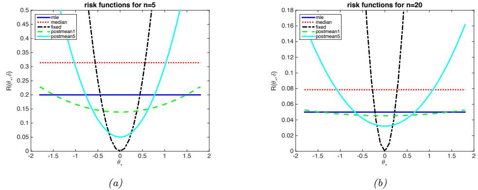
Figure 5.8: Risk functions for estimating the mean of a Gaussian. Each curve represents ^R(ˆεi(·), ^ε↔︎) plotted vs ^ε↔︎, where ⁱ indexes the estimator. Each estimator is applied to ^N samples from ^N (ε↔︎, ^ϑ2 = 1). The dark blue horizontal line is the sample mean (MLE); the red line horizontal line is the sample median; the black curved line is the estimator ˆε = ε⁰ = 0; the green curved line is the posterior mean when ⇁ = 1; the light blue curved line is the posterior mean when ⇁ = 5. (a) N = 5 samples. (b) N = 20 samples. Adapted from Figure B.1 of [BS94]. Generated by riskFnGauss.ipynb.

We now consider 5 di!erent estimators for computing ϖ:

• ↽1(x) = x, the sample mean.
• ↽2(x) = median(x), the sample median.
• ↽3(x) = ϖ0, a fixed value
• ↽κ(x), the posterior mean under a ^N (ϖ|ϖ0, ^ε2/2) prior:

\[\delta\_{\kappa}(\mathbf{x}) = \frac{N}{N+\kappa}\overline{x} + \frac{\kappa}{N+\kappa}\theta\_0 = w\overline{x} + (1-w)\theta\_0 \tag{5.65}\]

For ↽κ, we use ϖ⁰ = 0, and consider a weak prior, 2 = 1, and a stronger prior, 2 = 5.

Let ˆϖ = ˆϖ(x) = ↽(x) be the estimated parameter. The risk of this estimator is given by the MSE. In Section 4.7.6.3, we show that the MSE can be decomposed into squared bias plus variance:

\[\text{MSE}(\hat{\theta}|\theta^\*) = \mathbb{V}\left[\hat{\theta}\right] + \text{bias}^2(\hat{\theta}) \tag{5.66}\]

where the bias is defined as bias(ˆϖ) = E ^{ˆϖ ↑ ϖ↓} . We now use this expression to derive the risk for each estimator.

↽¹ is the sample mean. This is unbiased, so its risk is

\[\text{MSE}(\delta\_1 | \theta^\*) = \mathbb{V}\left[\overline{x}\right] = \frac{\sigma^2}{N} \tag{5.67}\]

↽² is the sample median. This is also unbiased. Furthermore, one can show that its variance is approximately ϑ/(2N) (where ϑ = 3.14) so the risk is

\[\text{MSE}(\delta\_2 | \theta^\*) = \frac{\pi}{2N} \tag{5.68}\]

↽³ returns the constant ϖ0, so its bias is (ϖ^↓ ↑ ϖ0) and its variance is zero. Hence the risk is

\[\text{MSE}(\delta\_3|\theta^\*) = (\theta^\* - \theta\_0)^2\tag{5.69}\]

Finally, ↽⁴ is the posterior mean under a Gaussian prior. We can derive its MSE as follows:

\[\text{MSE}(\delta\_{\kappa}|\theta^{\*}) = \mathbb{E}\left[\left(w\overline{x} + (1-w)\theta\_{0} - \theta^{\*}\right)^{2}\right] \tag{5.70}\]

\[=\mathbb{E}\left[\left(w(\overline{x}-\theta^\*)+(1-w)(\theta\_0-\theta^\*)\right)^2\right]\tag{5.71}\]

\[=w^2\frac{\sigma^2}{N} + (1-w)^2(\theta\_0 - \theta^\*)^2\tag{5.72}\]

\[=\frac{1}{(N+\kappa)^2} \left( N\sigma^2 + \kappa^2 (\theta\_0 - \theta^\*)^2 \right) \tag{5.73}\]

These functions are plotted in Figure 5.8 for N → {5, 20}. We see that in general, the best estimator depends on the value of ϖ↓, which is unknown. If ϖ^↓ is very close to ϖ0, then ↽³ (which just predicts ϖ0) is best. If ϖ^↓ is within some reasonable range around ϖ0, then the posterior mean, which combines the prior guess of ϖ⁰ with the actual data, is best. If ϖ^↓ is far from ϖ0, the MLE is best.

5.3.1.2 Bayes risk

In general, the true state of nature ω that generates the data x is unknown, so we cannot compute the risk given in Equation (5.64). One solution to this is to assume a prior ϑ⁰ for ω, and then average it out. This gives us the Bayes risk, also called the integrated risk:

\[R\_{\pi\_0}(\delta) \triangleq \mathbb{E}\_{\pi\_0(\theta)} \left[ R(\theta, \delta) \right] = \int d\theta \, dx \, \pi\_0(\theta) p(x|\theta) \ell(\theta, \delta(x)) \tag{5.74}\]

A decision rule that minimizes the Bayes risk is known as a Bayes estimator. This is equivalent to the optimal policy recommended by Bayesian decision theory in Equation (5.2) since

\[\delta(\mathbf{z}) = \operatorname\*{argmin}\_{a} \int d\theta \,\pi\_{0}(\theta) p(\mathbf{z}|\theta) \ell(\theta, a) = \operatorname\*{argmin}\_{a} \int d\theta \, p(\theta|\mathbf{z}) \ell(\theta, a) \tag{5.75}\]

Hence we see that picking the optimal action on a case-by-case basis (as in the Bayesian approach) is optimal on average (as in the frequentist approach). In other words, the Bayesian approach provides a good way of achieving frequentist goals. See [BS94, p448] for further discussion of this point.

5.3.1.3 Maximum risk

Of course the use of a prior might seem undesirable in the context of frequentist statistics. We can therefore define the maximum risk as follows:

\[R\_{\text{max}}(\delta) \stackrel{\Delta}{=} \sup\_{\theta} R(\theta, \delta) \tag{5.76}\]

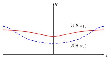
Figure 5.9: Risk functions for two decision procedures, ◁¹ and ◁2. Since ◁¹ has lower worst case risk, it is the minimax estimator, even though ◁² has lower risk for most values of ε. Thus minimax estimators are overly conservative.

A decision rule that minimizes the maximum risk is called a minimax estimator, and is denoted ↽MM. For example, in Figure 5.9, we see that ↽¹ has lower worst-case risk than ↽2, ranging over all possible values of ω, so it is the minimax estimator.

Minimax estimators have a certain appeal. However, computing them can be hard. And furthermore, they are very pessimistic. In fact, one can show that all minimax estimators are equivalent to Bayes estimators under a least favorable prior. In most statistical situations (excluding game theoretic ones), assuming nature is an adversary is not a reasonable assumption.

5.3.2 Consistent estimators

Suppose we have a dataset x = {xⁿ : n =1: N} where the samples xⁿ → X are generated iid from a distribution p(X|ω↓), where ω^↓ → # is the true parameter. Furthermore, suppose the parameters are identifiable, meaning that p(x|ω) = p(x|ω↗ ) i! ω = ω↗ for any dataset x. Then we say that an estimator ↽ : ^{X N ↔︎} # is a consistent estimator if ^ωˆ(x) ^{↔︎ ω↓} as ^N ↔︎ ∈ (where the arrow denotes convergence in probability). In other words, the procedure ↽ recovers the true parameter (or a subset of it) in the limit of infinite data. This is equivalent to minimizing the 0-1 loss, ^L(ω↓, ^ωˆ) = ^{I ω↓} ↗^{= ωˆ} . An example of a consistent estimator is the maximum likelihood estimator (MLE).

Note that an estimator can be unbiased but not consistent. For example, consider the estimator ↽(x) = ↽({x1,…, x^N }) = x^N . This is an unbiased estimator of the true mean µ, since E [↽(x)] = E [x^N ] = µ. But the sampling distribution of ↽(x) does not converge to a fixed value, so it cannot converge to the point ω↓.

Although consistency is a desirable property, it is of somewhat limited usefulness in practice since most real datasets do not come from our chosen model family (i.e., there is no ω^↓ such that p(·|ω↓) generates the observed data x). In practice, it is more useful to find estimators that minimize some discrepancy measure between the empirical distribution and the estimated distribution. If we use KL divergence as our discrepancy measure, our estimate becomes the MLE.

5.3.3 Admissible estimators

We say that ↽¹ dominates ↽² if R(ω, ↽1) ↘ R(ω, ↽2) for all ω. The domination is said to be strict if the inequality is strict for some ω↓. An estimator is said to be admissible if it is not strictly dominated by any other estimator. Interestingly, [Wal47] proved that all admissible decision rules are equivalent to some kind of Bayesian decision rule, under some technical conditions. (See [DR21]

for a more general version of this result.)

For example, in Figure 5.8, we see that the sample median (dotted red line) always has higher risk than the sample mean (solid blue line). Therefore the sample median is not an admissible estimator for the mean. More surprisingly, one can show that the sample mean is not always an admissible estimator either, even under a Gaussian likelihood model with squared error loss (this is known as Stein’s paradox [Ste56]).

However, the concept of admissibility is of somewhat limited value. For example, let X ⇒ N (ϖ, 1), and consider estimating ϖ under squared loss. Consider the estimator ↽1(x) = ϖ0, where ϖ⁰ is a constant independent of the data. We now show that this is an admissible estimator.

To see this, suppose it were not true. Then there would be some other estimator ↽² with smaller risk, so R(ϖ↓, ↽2) ↘ R(ϖ↓, ↽1), where the inequality must be strict for some ϖ↓. Consider the risk at ϖ^↓ = ϖ0. We have R(ϖ0, ↽1)=0, and

\[R(\theta\_0, \delta\_2) = \int (\delta\_2(x) - \theta\_0)^2 p(x|\theta\_0) dx \tag{5.77}\]

Since 0 ↘ R(ϖ↓, ↽2) ↘ R(ϖ↓, ↽1) for all ϖ↓, and R(ϖ0, ↽1)=0, we have R(ϖ0, ↽2)=0 and hence ↽2(x) = ϖ⁰ = ↽1(x). Thus the only way ↽² can avoid having higher risk than ↽¹ at ϖ⁰ is by being equal to ↽1. Hence there is no other estimator ↽² with strictly lower risk, so ↽² is admissible.

Thus we see that the estimator ↽1(x) = ϖ⁰ is admissible, even though it ignores the data, so is useless as an estimator. Conversely, it is possible to construct useful estimators that are not admissable (see e.g., [Jay03, Sec 13.7]).

5.4 Empirical risk minimization

In this section, we consider how to apply frequentist decision theory in the context of supervised learning.

5.4.1 Empirical risk

In standard accounts of frequentist decision theory used in statistics textbooks, there is a single unknown “state of nature”, corresponding to the unknown parameters ω^↓ of some model, and we define the risk as in Equation (5.64), namely R(↽, ω↓) = Ep(D|ω↑) [ω(ω↓, ↽(D))].

In supervised learning, we have a di!erent unknown state of nature (namely the output y) for each input x, and our estimator ↽ is a prediction function yˆ = f(x), and the state of nature is the true distribution p↓(x, y). Thus the risk of an estimator is as follows:

\[R(f, p^\*) = R(f) \stackrel{\Delta}{=} \mathbb{E}\_{p^\*(x)p^\*(y|x)}[\ell(y, f(x))]\tag{5.78}\]

This is called the population risk, since the expectations are taken wrt the true joint distribution p↓(x, y). Of course, p^↓ is unknown, but we can approximate it using the empirical distribution with N samples:

\[p\_{\mathcal{D}}(x, y | \mathcal{D}) \stackrel{\scriptstyle \Delta}{=} \frac{1}{|\mathcal{D}|} \sum\_{(\mathfrak{x}\_n, \mathfrak{y}\_n) \in \mathcal{D}} \delta(x - x\_n) \delta(y - y\_n) \tag{5.79}\]

where pD(x, y) = ptr(x, y). Plugging this in gives us the empirical risk:

\[R(f, \mathcal{D}) \triangleq \mathbb{E}\_{p\_{\mathcal{D}}(\mathbf{z}, \mathbf{y})} \left[ \ell(\mathbf{y}, f(\mathbf{z})) \right] = \frac{1}{N} \sum\_{n=1}^{N} \ell(\mathbf{y}\_n, f(\mathbf{z}\_n)) \tag{5.80}\]

Note that R(f, D) is a random variable, since it depends on the training set.

A natural way to choose the predictor is to use

\[\hat{f}\_{\text{ERM}} = \operatorname\*{argmin}\_{f \in \mathcal{H}} R(f, \mathcal{D}) = \operatorname\*{argmin}\_{f \in \mathcal{H}} \frac{1}{N} \sum\_{n=1}^{N} \ell(y\_n, f(x\_n)) \tag{5.81}\]

where we optimize over a specific hypothesis space H of functions. This is called empirical risk minimization (ERM).

5.4.1.1 Approximation error vs estimation error

In this section, we analyze the theoretical performance of functions that are fit using the ERM principle. Let f ↓↓ = argmin^f R(f) be the function that achieves the minimal possible population risk, where we optimize over all possible functions. Of course, we cannot consider all possible functions, so let us also define f ^{↓ H} = argmin^f↑^H R(f) to be the best function in our hypothesis space, H. Unfortunately we cannot compute f ^{↓ H}, since we cannot compute the population risk, so let us finally define the prediction function that minimizes the empirical risk in our hypothesis space, given a fixed training set D:

\[f\_{\mathcal{D}}^{\*} = \operatorname\*{argmin}\_{f \in \mathcal{H}} R(f, \mathcal{D}) \tag{5.82}\]

This is a random function, since D ⇒ p^↓ is random.

By adding and substracting terms, we can show that the expected risk of our chosen predictor compared to the best possible predictor can be decomposed into two terms, as follows:

\[\mathbb{E}\_{\mathcal{D}\sim p^\*}\left[R(f\_{\mathcal{D}}^\*)-R(f^{\*\*})\right] = \underbrace{R(f\_{\mathcal{H}}^\*)-R(f^{\*\*})}\_{\mathcal{E}\_{\text{app}}(\mathcal{H})} + \underbrace{\mathbb{E}\_{\mathcal{D}\sim p^\*}\left[R(f\_{\mathcal{D}}^\*)-R(f\_{\mathcal{H}}^\*)\right]}\_{\mathcal{E}\_{\text{auf}}(\mathcal{H},N)}\tag{5.83}\]

The first term, Eapp(H), is the approximation error, which measures how closely f ^{↓ H} can model the true optimal function f ↓↓. The second term, Eest(H, N), is the estimation error, which measures the error in finding the best function in the class, due to having a finite training set of size N to evaluate performance. (One can also study the extra error introduced by the training process [BB08].)

We can decrease the approximation error by using a more expressive family of functions H. However, this usually increases overfitting, which increases the estimation error. We can quantify the degree of overfitting of any model f by computing the generalization gap, defined as follows:

\[\text{GenGap}(f) = R(f) - R(f, \mathcal{D}\_{\text{train}}) \approx R(f, \mathcal{D}\_{\text{test}}) - R(f, \mathcal{D}\_{\text{train}}) \tag{5.84}\]

Thus we need to find models that tradeo! approximation error and estimation error. We discuss solutions to this tradeo! below.

5.4.1.2 Regularized risk

To avoid the chance of overfitting, it is common to add a complexity penalty to the objective function, giving us the regularized empirical risk:

\[R\lambda(f,\mathcal{D}) = R(f,\mathcal{D}) + \lambda C(f) \tag{5.85}\]

where C(f) measures the complexity of the prediction function f(x; ω), and φ ∋ 0, which is known as a hyperparameter, controls the strength of the complexity penalty. (We discuss how to pick φ in Section 5.4.2.)

In practice, we usually work with parametric functions, and apply the regularizer to the parameters themselves. This yields the following form of the objective:

\[R\_{\lambda}(\theta, \mathcal{D}) = R(\theta, \mathcal{D}) + \lambda C(\theta) \tag{5.86}\]

Note that, if the loss function is log loss, and the regularizer is a negative log prior, the regularized risk is given by

\[R\_{\lambda}(\theta, \mathcal{D}) = -\frac{1}{N} \sum\_{n=1}^{N} \log p(y\_n | x\_n, \theta) - \lambda \log p(\theta) \tag{5.87}\]

Minimizing this is equivalent to MAP estimation.

5.4.2 Structural risk

A natural way to estimate the hyperparameters is to minimize for the lowest achievable empirical risk:

\[\hat{\lambda} = \operatorname\*{argmin}\_{\lambda} \min\_{\theta} R\_{\lambda}(\theta, \mathcal{D}) \tag{5.88}\]

(This is an example of bilevel optimization, also called nested optimization.) Unfortunately, this technique will not work, since it will always pick the least amount of regularization, i.e., φˆ = 0. To see this, note that

\[\underset{\lambda}{\text{argmin}} \min\_{\theta} R\_{\lambda}(\theta, \mathcal{D}) = \underset{\lambda}{\text{argmin}} \min\_{\theta} R(\theta, \mathcal{D}) + \lambda C(\theta) \tag{5.89}\]

which is minimized by setting φ = 0. The problem is that the empirical risk underestimates the population risk, resulting in overfitting when we choose φ. This is called optimism of the training error.

If we knew the regularized population risk R↼(ω), instead of the regularized empirical risk R↼(ω, D), we could use it to pick a model of the right complexity (e.g., value of φ). This is known as structural risk minimization [Vap98]. There are two main ways to estimate the population risk for a given model (value of φ), namely cross-validation (Section 5.4.3), and statistical learning theory (Section 5.4.4), which we discuss below.

5.4.3 Cross-validation

In this section, we discuss a simple way to estimate the population risk for a supervised learning setup. We simply partition the dataset into two, the part used for training the model, and a second part, called the validation set or holdout set, used for assessing the risk. We can fit the model on the training set, and use its performance on the validation set as an approximation to the population risk.

To explain the method in more detail, we need some notation. First we make the dependence of the empirical risk on the dataset more explicit as follows:

\[R\_{\lambda}(\theta, \mathcal{D}) = \frac{1}{|\mathcal{D}|} \sum\_{(x, y) \in \mathcal{D}} \ell(y, f(x; \theta)) + \lambda C(\theta) \tag{5.90}\]

Let us also define ^ωˆ↼(D) = argmin^{ω R}↼(D, ^ω). Finally, let ^Dtrain and ^Dvalid be a partition of ^D. (Often we use about 80% of the data for the training set, and 20% for the validation set.)

For each model ^φ, we fit it to the training set to get ^ωˆ↼(Dtrain). We then use the unregularized empirical risk on the validation set as an estimate of the population risk. This is known as the validation risk:

\[R\_{\lambda}^{\text{val}} \triangleq R\_0(\hat{\boldsymbol{\theta}}\_{\lambda}(\mathcal{D}\_{\text{train}}), \mathcal{D}\_{\text{valid}}) \tag{5.91}\]

Note that we use di!erent data to train and evaluate the model.

The above technique can work very well. However, if the number of training cases is small, this technique runs into problems, because the model won’t have enough data to train on, and we won’t have enough data to make a reliable estimate of the future performance.

A simple but popular solution to this is to use cross validation (CV). The idea is as follows: we split the training data into K folds; then, for each fold k → {1,…,K}, we train on all the folds but the k’th, and test on the k’th, in a round-robin fashion, as sketched in Figure 4.6. Formally, we have

\[R\_{\lambda}^{\text{cv}} \stackrel{\Delta}{=} \frac{1}{K} \sum\_{k=1}^{K} R\_0(\hat{\theta}\_{\lambda}(\mathcal{D}\_{-k}), \mathcal{D}\_k) \tag{5.92}\]

where D^k is the data in the k’th fold, and D→^k is all the other data. This is called the cross-validated risk. Figure 4.6 illustrates this procedure for K = 5. If we set K = N, we get a method known as leave-one-out cross-validation, since we always train on N ↑ 1 items and test on the remaining one.

We can use the CV estimate as an objective inside of an optimization routine to pick the optimal hyperparameter, ^{φˆ =} argmin↼ ^Rcv ↼ . Finally we combine all the available data (training and validation), and re-estimate the model parameters using ^ωˆ = argmin^{ω R}↼^ˆ(ω, ^D).

5.4.4 Statistical learning theory *

The principal problem with cross validation is that it is slow, since we have to fit the model multiple times. This motivates the desire to compute analytic approximations or bounds on the population risk. This is studied in the field of statistical learning theory (SLT) (see e.g., [Vap98]).

More precisely, the goal of SLT is to upper bound the generalization error with a certain probability. If the bound is satisfied, then we can be confident that a hypothesis that is chosen by minimizing the empirical risk will have low population risk. In the case of binary classifiers, this means the hypothesis will make the correct predictions; in this case we say it is probably approximately correct, and that the hypothesis class is PAC learnable (see e.g., [KV94] for details).

5.4.4.1 Bounding the generalization error

In this section, we establish conditions under which we can prove that a hypothesis class is PAC learnable. Let us initially consider the case where the hypothesis space is finite, with size dim(H) = |H|. In other words, we are selecting a hypothesis from a finite list, rather than optimizing real-valued parameters. In this case, we can prove the following.

Theorem 5.4.1. For any data distribution p↓, and any dataset D of size N drawn from p↓, the probability that the generalization error of a binary classifier will be more than ▷, in the worst case, is upper bounded as follows:

\[P\left(\max\_{h\in\mathcal{H}}|R(h)-R(h,\mathcal{D})|>\epsilon\right)\leq2\dim(\mathcal{H})e^{-2Ne^{2}}\tag{5.93}\]

where ^R(h, ^D) = ¹ N $^{N i}=1 I(f(xi) ↗= y^{↓ i} ) is the empirical risk, and R(h) = E [I(f(x) ↗= y↓)] is the population risk.

Proof. Before we prove this, we introduce two useful results. First, Hoe”ding’s inequality, which states that if E1,…,E^N ⇒ Ber(ϖ), then, for any ▷ > 0,

\[P(|\overline{E} - \theta| > \epsilon) \le 2e^{-2N\epsilon^2} \tag{5.94}\]

where E = ¹ N $^{N i}=1 Eⁱ is the empirical error rate, and ϖ is the true error rate. Second, the union bound, which says that if ^A1,…,A^d are a set of events, then ^P(∀^{d i}=1Ai) ↘ $^{d i}=1 P(Ai). Using these results, we have

\[P\left(\max\_{h\in\mathcal{H}}|R(h)-R(h,\mathcal{D})|>\epsilon\right)=P\left(\bigcup\_{h\in\mathcal{H}}|R(h)-R(h,\mathcal{D})|>\epsilon\right)\tag{5.95}\]

\[\epsilon \le \sum\_{h \in \mathcal{H}} P\left( |R(h) - R(h, \mathcal{D})| > \epsilon \right) \tag{5.96}\]

\[\leq \sum\_{h \in \mathcal{H}} 2e^{-2Ne^2} = 2 \dim(\mathcal{H}) e^{-2Ne^2} \tag{5.97}\]

This bound tells us that the optimism of the training error increases with dim(H) but decreases with N = |D|, as is to be expected.

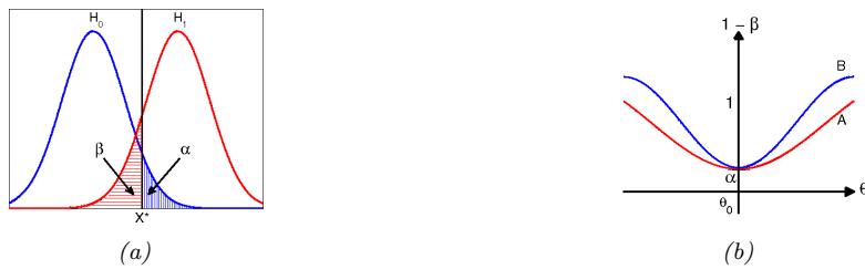
Figure 5.10: (a) Illustration of the Neyman-Pearson hypothesis testing paradigm. Generated by neyman-Pearson2.ipynb. (b) Two hypothetical two-sided power curves. B dominates A. Adapted from Figure 6.3.5 of [LM86]. Generated by twoPowerCurves.ipynb.

5.4.4.2 VC dimension

If the hypothesis space H is infinite (e.g., we have real-valued parameters), we cannot use dim(H) = |H|. Instead, we can use a quantity called the VC dimension of the hypothesis class, named after Vapnik and Chervonenkis; this measures the degrees of freedom (e!ective number of parameters) of the hypothesis class. See e.g., [Vap98] for the details.

Unfortunately, it is hard to compute the VC dimension for many interesting models, and the upper bounds are usually very loose, making this approach of limited practical value. However, various other, more practical, estimates of generalization error have recently been devised, especially for DNNs, such as [Jia+20].

5.5 Frequentist hypothesis testing *

In this section, we discuss ways to determining if a hypothesis (model) is plausible or not, in the light of data D.

5.5.1 Likelihood ratio test

When deciding if a model is a good description of some data or not, it is always useful to ask “relative to what”. To make this concrete, suppose we have two hypotheses, known as the null hypothesis H⁰ and an alternative hypothesis H1, and we want to choose the one we think is more likely. We can think of this as a binary classification problem, where H → {0, 1} represents the identity of the “true” model. A natural approach is to use Bayesian model selection, as we discussed in Section 5.2.1, to compute p(H|D), and then to pick the most probable model. Here we discuss a frequentist approach.

Suppose we have a uniform prior, so p(H = 0) = p(H = 1) = 0.5, and that we use 0-1 loss. Then the optimal decision rule is to accept H⁰ i! ^p(D|H0) ^p(D|H1) ^&gt; ¹. This is called the likelihood ratio test. We give some examples of this below.

5.5.1.1 Example: comparing Gaussian means

Suppose we are interested in testing whether some data comes from a Gaussian with mean µ⁰ or from a Gaussian with mean µ1. (We assume a known shared variance ε².) This is illustrated in

Figure 5.10a, where we plot p(x|H0) and p(x|H1). We can derive the likelihood ratio as follows:

\[\frac{p(\mathcal{D}|H\_0)}{p(\mathcal{D}|H\_1)} = \frac{\exp\left(-\frac{1}{2\sigma^2} \sum\_{n=1}^N (x\_n - \mu\_0)^2\right)}{\exp\left(-\frac{1}{2\sigma^2} \sum\_{n=1}^N (x\_n - \mu\_1)^2\right)}\tag{5.98}\]

\[=\exp\left(\frac{1}{2\sigma^2}(2N\overline{x}(\mu\_0-\mu\_1)+N\mu\_1^2-N\mu\_0^2)\right)\tag{5.99}\]

We see that this ratio only depends on the observed data via its mean, x. From Figure 5.10a, we can see that ^p(D|H0) ^p(D|H1) ^&gt; ^{1 i}! x<x↓, where ^x↓ is the point where the two pdf’s intersect (we are assuming this point is unique).

5.5.1.2 Simple vs compound hypotheses

In Section 5.5.1.1, the parameters for the null and alternative hypotheses were either fully specified (µ⁰ and µ1) or shared (ε²). This is called a simple hypothesis test. In general, a hypothesis might not fully specify all the parameters; this is called a compound hypothesis. In this case, we could integrate out these unknown parameters, as in the Bayesian approach, since a hypothesis with more parameters will always have higher likelihood. However, this can be computationally di”cult, and is prone to problems caused by prior misspecification. As an alternative approach, we can “maximize out” the parameters, which gives us the maximum likelihood ratio test:

\[\frac{p(H\_0|\mathcal{D})}{p(H\_1|\mathcal{D})} = \frac{\int\_{\theta \in H\_0} p(\theta)p\_\theta(\mathcal{D})}{\int\_{\theta \in H\_1} p(\theta)p\_\theta(\mathcal{D})} \approx \frac{\max\_{\theta \in H\_0} p\_\theta(\mathcal{D})}{\max\_{\theta \in H\_1} p\_\theta(\mathcal{D})}\tag{5.100}\]

5.5.2 Type I vs type II errors and the Neyman-Pearson lemma

Hypothesis testing is a kind of binary classification problem. As we discussed in Section 5.1.3, there are two kinds of error we can make, known as a false positive or type I error, which corresponds to accidentally accepting the alterative when the null is true (i.e, ^p(H^ˆ = 1|^H = 0)), and a false negative or type II error, which corresponds to accidentally accepting the null when the alternative is true (i.e, ^p(H^ˆ = 0|^H = 1)). The type I error rate ^ϱ is called the significance of the test. In our Gaussian mean example, we see from Figure 5.10a that the type I error rate is the vertical shaded blue area:

\[\alpha(\mu\_0) = p(\text{type I error}) = p(\text{reject } H\_0 | H\_0 \text{ is true}) \tag{5.101}\]

\[=p(\overline{X}(\tilde{\mathcal{D}}) > x^\* | \tilde{\mathcal{D}} \sim H\_0) \tag{5.102}\]

\[\mu = p \left( \frac{\overline{X} - \mu\_0}{\sigma / \sqrt{N}} > \frac{x^\* - \mu\_0}{\sigma / \sqrt{N}} \right) \tag{5.103}\]

Hence x^↓ = z↽ε/ ≃ N + µ0, where z↽ is the upper ϱ quantile of the standard Normal. The type II error rate is denoted by 1, and is given by

\[p(\beta\_1) = p(\text{type II error}) = p(\text{accept } H\_0 | H\_1 \text{ is true}) = p(\overline{X} | \tilde{\mathcal{D}}) < x^\* | \tilde{\mathcal{D}} \sim H\_1) \tag{5.104}\]

This is shown by the horizontal shaded red area in Figure 5.10a.

We define the power of a test as 1 ↑ 1(µ1); this is the probability that we reject H⁰ given that ^H1 is true (i.e, ^p(H^ˆ = 1|^H = 1), which is the true positive rate). In other words, it is the ability to correctly recognize that the null hypothesis is wrong. Clearly the least power occurs if µ¹ = µ⁰ (so the curves overlap); in this case, we have 1 ↑ 1(µ1) = ϱ(µ0). As µ¹ and µ⁰ become further apart, the power approaches 1 (because the shaded red area gets smaller, 1 ↔︎ 0). If we have two tests, A and B, where power(B) ∋ power(A) for the same type I error rate, we say B dominates A. See Figure 5.10b. A test with highest power under H¹ amongst all tests with significance level ϱ is called a most powerful test. It turns out that the likelihood ratio test is a most powerful test, a result known as the Neyman-Pearson lemma.

5.5.3 Null hypothesis significance testing (NHST) and p-values

In the above decision-theoretic (or Neyman-Pearson) approach to hypothesis testing, we had to specify a null hypothesis H⁰ as well as an alternative hypothesis H¹ so that we can compute p(D|H0) and p(D|H1). In some cases, it is di”cult to define an alternative hypothesis, and we just want to test if a simple null hypothesis is “plausible” given some data. To do this, we can define a test statistic test(D), and then we can compare its observed value to the value we would expect if the data came from the null hypothesis, test(D˜ ) where ^D˜ ^{⇒ H}0. If the observed value is unexpected given H0, we reject the null hypothesis. To quantify this, we compute the probability of seeing a test value that is as large or larger than the observed value (assuming that larger values make H¹ more likely). More precisely, we define the p-value to be the probability, under the null hypothesis, of observing a test statistic that is as large or larger than that actually observed:

\[\text{pval} \triangleq \Pr(\text{test}(\tilde{\mathcal{D}}) \ge \text{test}(\mathcal{D}) | \tilde{\mathcal{D}} \sim H\_0) \tag{5.105}\]

In other words, pval ↭ Pr(testnull ^∋ testobs), where testobs ⁼ test(D) and testnull ⁼ test(D˜ ), where ^D˜ ^{⇒ H0} is hypothetical future data. Smaller values correspond to stronger evidence against ^H0.

Traditionally we reject the null hypothesis if the p-value is less than ϱ = 0.05; this is called the significance level of the test, and the whole approach is called null hypothesis significance testing or NHST. By construction, such a test will have a type I error rate (accidently rejecting the null when it is true) of value ϱ. Note that this decision rule corresponds to picking decision threshold t ^↓ such that Pr(test(D˜ ) ^{∋ t ↓}|H0) = ϱ. If we set t ^↓ = test(D), then ϱ will be equal to the observed p-value. Thus the p-value is the smallest value of ϱ for which we can reject H0.

We can compute the p-value using pval = 1 ↑ !(test(D)), where ! is the cdf of the sampling distribution of the test statistic. This is called a one-sided p-value. In some case it can be more appropriate to use a two-sided p-value of the form pval ⁼ Pr(test(D˜ ) ^∋ test(D)|D˜ ^{⇒ H}0)+Pr(test(D˜ ) ↘ ↑test(D)|D˜ ^{⇒ H}0), where we have assumed test(D) ^{∋ 0}. For example, suppose we use test(D˜ )=(ˆϖ(D˜ )↑ϖ0)/ ˆse(D˜ ), where ^ϖ0 is the value for ^ϖ↓ given ^H0, and ^ˆϖ is the MLE; ths is known as the Wald statistic. Based on the asymptotic normality of the MLE discussed in Section 4.7.2, we have that pval ⁼ Pr(|test(D˜ )^{| &}gt; ^|test(D)| | ^H0) ↖ Pr(|Z^{| &}gt; ^|test(D)|) = 2!(↑|test(D)|), where Z ⇒ N (0, 1).

We see that, to compute the p-value, we need to compute the sampling distribution of the test statistic under the null hypothesis. Suppose we want to compare an empirical distribution or outcome to an expected (theoretical) distribution or outcome. In some cases we can use a large sample (Gaussian approxmation) to the sampling distribution, as we illustrated above. If not, we can use a non-parametric bootstrap approximation. Another important case arises when we want to compare

two empirical distributions to test if they are the same; for this we can use the non-parametric permutation test, which makes no assumptions about the distribution. For example, suppose we have m samples Xⁱ from P^X and n samples Yⁱ from P^y and the null hypothesis is P^x = Py. Define the test statistic test(X1,…,Xm, Y1,…,Yn) = |X ↑ Y |. If we permute the order of the samples, then, under H0, this statistic should not change. So we can sample random permutations to approximate ^p(test(D˜ )|D˜ ^{⇒ H}0), from which we can compute the tail probability of test(D) computed using the unshu#ed data. For more details, see e.g. [Was04, p162].

Note that a p-value of 0.05 does not mean that the alternative hypothesis H¹ is true with probability 0.95. Indeed, even most scientists misinterpret p-values.4 The quantity that most people want to compute is the Bayesian posterior p(H|D). For more on this important distinction, see Section 5.5.4.

5.5.4 p-values considered harmful

A p-value is often interpreted as the likelihood of the data under the null hypothesis, so small values are interpreted to mean that H⁰ is unlikely, and therefore that H¹ is likely. The reasoning is roughly as follows:

If H⁰ is true, then this test statistic would probably not occur. This statistic did occur. Therefore H⁰ is probably false.

However, this is invalid reasoning. To see why, consider the following example (from [Coh94]):

If a person is an American, then he is probably not a member of Congress. This person is a member of Congress. Therefore he is probably not an American.

This is obviously fallacious reasoning. By contrast, the following logical argument is valid reasoning:

If a person is a Martian, then he is not a member of Congress. This person is a member of Congress. Therefore he is not a Martian.

The di!erence between these two cases is that the Martian example is using deduction, that is, reasoning forward from logical definitions to their consequences. More precisely, this example uses a rule from logic called modus tollens, in which we start out with a definition of the form P ∝ Q; when we observe ¬Q, we can conclude ¬P. By contrast, the American example concerns induction, that is, reasoning backwards from observed evidence to probable (but not necessarily true) causes using statistical regularities, not logical definitions.

To perform induction, we need to use probabilistic inference (as explained in detail in [Jay03]). In particular, to compute the probability of the null hypothesis, we should use Bayes rule, as follows:

\[p(H\_0|\mathcal{D}) = \frac{p(\mathcal{D}|H\_0)p(H\_0)}{p(\mathcal{D}|H\_0)p(H\_0) + p(\mathcal{D}|H\_1)p(H\_1)}\tag{5.106}\]

If the prior is uniform, so p(H0) = p(H1)=0.5, this can be rewritten in terms of the likelihood ratio LR = p(D|H0)/p(D|H1) as follows:

\[p(H\_0|\mathcal{D}) = \frac{LR}{LR+1} \tag{5.107}\]

^4. See e.g., https://fivethirtyeight.com/features/not-even-scientists-can-easily-explain-p-values/.

	Ine!ective	E!ective
“Not significant”	171	4	175
“Significant”	9	16	25
	180	20	200

Table 5.8: Some statistics of a hypothetical clinical trial. Source: [SAM04, p74].

In the American Congress example, D is the observation that the person is a member of Congress. The null hypothesis H⁰ is that the person is American, and the alternative hypothesis H¹ is that the person is not American. We assume that p(D|H0) is low, since most Americans are not members of Congress. However, p(D|H1) is also low — in fact, in this example, it is 0, since only Americans can be members of Congress. Hence LR = ∈, so p(H0|D)=1.0, as intuition suggests. Note, however, that NHST ignores p(D|H1) as well as the prior p(H0), so it gives the wrong results — not just in this problem, but in many problems.

In general there can be huge di!erences between p-values and p(H0|D). In particular, [SBB01] show that even if the p-value is as low as 0.05, the posterior probability of H⁰ can be as high as 30% or more, even with a uniform prior.

Consider this concrete example from [SAM04, p74]. Suppose 200 clinical trials are carried out for some drug, and we get the data in Table 5.8. Suppose we perform a statistical test of whether the drug has a significant e!ect or not. The test has a type I error rate of ϱ = 9/180 = 0.05 and a type II error rate of 1 = 4/20 = 0.2.

We can compute the probability that the drug is not e!ective, given that the result is supposedly “significant”, as follows:

\[p(H\_0|\text{'significant'}) = \frac{p(\text{'significant'}|H\_0)p(H\_0)}{p(\text{'significant'}|H\_0)p(H\_0) + p(\text{'significant'}|H\_1)p(H\_1)}\tag{5.108}\]

\[t = \frac{p(\text{type I error})p(H\_0)}{p(\text{type I error})p(H\_0) + (1 - p(\text{type II error}))p(H\_1)}\tag{5.109}\]

\[=\frac{\alpha p(H\_0)}{\alpha p(H\_0) + (1-\beta)p(H\_1)}\tag{5.110}\]

If we have prior knowledge, based on past experience, that most (say 90%) drugs are ine!ective, then we find p(H0|’significant’)=0.36, which is much more than the 5% probability people usually associate with a p-value of ϱ = 0.05.

Thus we should distrust claims of statistical significance if they violate our prior knowledge.

5.5.5 Why isn’t everyone a Bayesian?

In Section 4.7.5 and Section 5.5.4, we have seen that inference based on frequentist principles can exhibit various forms of counter-intuitive behavior that can sometimes contradict common sense reason, as has been pointed out in multiple articles (see e.g., [Mat98; MS11; Kru13; Gel16; Hoe+14; Lyu+20; Cha+19b; Cla21]).

The fundamental reason for these problems is that frequentist inference violates the likelihood principle [BW88], which says that inference should be based on the likelihood of the observed data,

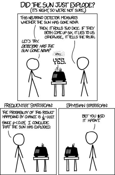
Figure 5.11: Cartoon illustrating the di!erence between frequentists and Bayesians. (The p < 0.05 comment is explained in Section 5.5.4. The betting comment is a reference to the Dutch book theorem, which essentially proves that the Bayesian approach to gambling (and other decision theory problems) is optimal, as explained in e.g., [Háj08].) From https: // xkcd. com/ 1132/ . Used with kind permission of Rundall Munroe (author of xkcd).

not on hypothetical future data that you have not observed. Bayes obviously satisfies the likelihood principle, and consequently does not su!er from these pathologies.

Given these fundamental flaws of frequentist statistics, and the fact that Bayesian methods do not have such flaws, an obvious question to ask is: “Why isn’t everyone a Bayesian?” The (frequentist) statistician Bradley Efron wrote a paper with exactly this title [Efr86]. His short paper is well worth reading for anyone interested in this topic. Below we quote his opening section:

The title is a reasonable question to ask on at least two counts. First of all, everyone used to be a Bayesian. Laplace wholeheartedly endorsed Bayes’s formulation of the inference problem, and most 19th-century scientists followed suit. This included Gauss, whose statistical work is usually presented in frequentist terms.

A second and more important point is the cogency of the Bayesian argument. Modern statisticians, following the lead of Savage and de Finetti, have advanced powerful theoretical arguments for preferring Bayesian inference. A byproduct of this work is a disturbing catalogue of inconsistencies in the frequentist point of view.

Nevertheless, everyone is not a Bayesian. The current era (1986) is the first century in which statistics has been widely used for scientific reporting, and in fact, 20th-century statistics is mainly non-Bayesian. However, Lindley (1975) predicts a change for the 21st century.

Time will tell whether Lindley was right. However, the trends seem to be going in this direction.

For example, some journals have banned p-values [TM15; AGM19], and the journal The American Statistician (produced by the American Statistical Association) published a whole special issue warning about the use of p-values and NHST [WSL19].

Traditionally, computation has been a barrier to using Bayesian methods, but this is less of an issue these days, due to faster computers and better algorithms (which we will discuss in the sequel to this book, [Mur23]). Another, more fundamental, concern is that the Bayesian approach is only as correct as its modeling assumptions. However, this criticism also applies to frequentist methods, since the sampling distribution of an estimator must be derived using assumptions about the data generating mechanism. (In fact [BT73] show that the sampling distributions for the MLE for common models are identical to the posterior distributions under a noninformative prior.) Fortunately, we can check modeling assumptions empirically using cross validation (Section 4.5.5), calibration, and Bayesian model checking. We discuss these topics in the sequel to this book, [Mur23].

To summarize, it is worth quoting Donald Rubin, who wrote a paper [Rub84] called “Bayesianly Justifiable and Relevant Frequency Calculations for the Applied Statistician”. In it, he writes

The applied statistician should be Bayesian in principle and calibrated to the real world in practice. [They] should attempt to use specifications that lead to approximately calibrated procedures under reasonable deviations from [their assumptions]. [They] should avoid models that are contradicted by observed data in relevant ways — frequency calculations for hypothetical replications can model a model’s adequacy and help to suggest more appropriate models.

5.6 Exercises

Exercise 5.1 [Reject option in classifiers]

(Source: [DHS01, Q2.13].) In many classification problems one has the option either of assigning x to class j or, if you are too uncertain, of choosing the reject option. If the cost for rejects is less than the cost of falsely classifying the object, it may be the optimal action. Let ωⁱ mean you choose action i, for i =1: C + 1, where C is the number of classes and C + 1 is the reject action. Let Y = j be the true (but unknown) state of nature. Define the loss function as follows

\[\lambda(\alpha\_l | Y = j) = \begin{cases} 0 & \text{if } i = j \text{ and } i, j \in \{1, \ldots, C\} \\ \lambda\_r & \text{if } i = C + 1 \\ \lambda\_s & \text{otherwise} \end{cases} \tag{5.111}\]

In other words, you incur 0 loss if you correctly classify, you incur ↼^r loss (cost) if you choose the reject option, and you incur ↼^s loss (cost) if you make a substitution error (misclassification).

• 1. Show that the minimum risk is obtained if we decide Y = j if p(Y = j|x) ↖ p(Y = k|x) for all k (i.e., j is the most probable class) and if ^p(^{Y = j}|x) ↖ ^{1 ↑ ϑr ϑs} ; otherwise we decide to reject.
• 2. Describe qualitatively what happens as ↼r/↼^s is increased from 0 to 1 (i.e., the relative cost of rejection increases).

Exercise 5.2 [Newsvendor problem † ]

Consider the following classic problem in decision theory / economics. Suppose you are trying to decide how much quantity Q of some product (e.g., newspapers) to buy to maximize your profits. The optimal amount will depend on how much demand D you think there is for your product, as well as its cost to you C and its selling price P. Suppose D is unknown but has pdf f(D) and cdf F(D). We can evaluate the expected profit by considering two cases: if D>Q, then we sell all Q items, and make profit ς = (P ↑ C)Q; but if D<Q,

we only sell D items, at profit (P ↑ C)D, but have wasted C(Q ↑ D) on the unsold items. So the expected profit if we buy quantity Q is

\[E\pi(Q) = \int\_{Q}^{\infty} (P - C)Qf(D)dD + \int\_{0}^{Q} (P - C)Df(D)dD - \int\_{0}^{Q} C(Q - D)f(D)dD\tag{5.112}\]

Simplify this expression, and then take derivatives wrt Q to show that the optimal quantity Q^↔︎ (which maximizes the expected profit) satisfies

\[F(Q^\*) = \frac{P - C}{P} \tag{5.113}\]

Exercise 5.3 [Bayes factors and ROC curves † ]

Let B = p(D|H1)/p(D|H0) be the Bayes factor in favor of model 1. Suppose we plot two ROC curves, one computed by thresholding B, and the other computed by thresholding p(H1|D). Will they be the same or di”erent? Explain why.

Exercise 5.4 [Posterior median is optimal estimate under L1 loss]

Prove that the posterior median is the optimal estimate under L1 loss.

6 Information Theory

In this chapter, we introduce a few basic concepts from the field of information theory. More details can be found in other books such as [Mac03; CT06], as well as the sequel to this book, [Mur23].

6.1 Entropy

The entropy of a probability distribution can be interpreted as a measure of uncertainty, or lack of predictability, associated with a random variable drawn from a given distribution, as we explain below.

We can also use entropy to define the information content of a data source. For example, suppose we observe a sequence of symbols Xⁿ ⇒ p generated from distribution p. If p has high entropy, it will be hard to predict the value of each observation Xn. Hence we say that the dataset D = (X1,…,Xn) has high information content. By contrast, if p is a degenerate distribution with 0 entropy (the minimal value), then every Xⁿ will be the same, so D does not contain much information. (All of this can be formalized in terms of data compression, as we discuss in the sequel to this book.)

6.1.1 Entropy for discrete random variables

The entropy of a discrete random variable X with distribution p over K states is defined by

\[\mathbb{H}\left(X\right) \triangleq -\sum\_{k=1}^{K} p(X=k)\log\_{2} p(X=k) = -\mathbb{E}\_{X}\left[\log p(X)\right] \tag{6.1}\]

(Note that we use the notation H (X) to denote the entropy of the rv with distribution p, just as people write V [X] to mean the variance of the distribution associated with X; we could alternatively write H (p).) Usually we use log base 2, in which case the units are called bits (short for binary digits). For example, if X → {1,…, 5} with histogram distribution p = [0.25, 0.25, 0.2, 0.15, 0.15], we find H = 2.29 bits. If we use log base e, the units are called nats.

The discrete distribution with maximum entropy is the uniform distribution. Hence for a K-ary random variable, the entropy is maximized if p(x = k)=1/K; in this case, H (X) = log² K. To see this, note that

\[\mathbb{H}\left(X\right) = -\sum\_{k=1}^{K} \frac{1}{K} \log(1/K) = -\log(1/K) = \log(K) \tag{6.2}\]

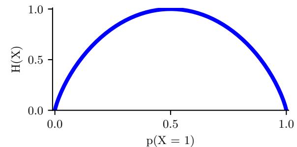
Figure 6.1: Entropy of a Bernoulli random variable as a function of ε. The maximum entropy is log² 2=1. Generated by bernoulli\_entropy\_fig.ipynb.

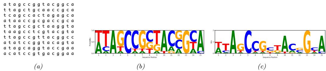
Figure 6.2: (a) Some aligned DNA sequences. Each row is a sequence, each column is a location within the sequence. (b) The corresponding position weight matrix, visualized as a sequence of histograms. Each column represents a probability distribution over the alphabet {A, C, G, T} for the corresponding location in the sequence. The size of the letter is proportional to the probability. (c) A sequence logo. See text for details. Generated by seq\_logo\_demo.ipynb.

Conversely, the distribution with minimum entropy (which is zero) is any delta-function that puts all its mass on one state. Such a distribution has no uncertainty.

For the special case of binary random variables, X → {0, 1}, we can write p(X = 1) = ϖ and p(X = 0) = 1 ↑ ϖ. Hence the entropy becomes

\[\mathbb{H}(X) = -[p(X=1)\log\_2 p(X=1) + p(X=0)\log\_2 p(X=0)]\tag{6.3}\]

\[=-\left[\theta\log\_2\theta+(1-\theta)\log\_2(1-\theta)\right] \tag{6.4}\]

This is called the binary entropy function, and is also written H (ϖ). We plot this in Figure 6.1. We see that the maximum value of 1 bit occurs when the distribution is uniform, ϖ = 0.5. A fair coin requires a single yes/no question to determine its state.

6.1.1.1 Application: DNA sequence logos

As an interesting application of entropy, consider the problem of representing DNA sequence motifs, which is a distribution over short DNA strings. We can estimate this distribution by aligning a set of DNA sequences (e.g., from di!erent species), and then estimating the empirical distribution of each possible nucleotide from the 4 letter alphabet X ⇒ {A, C, G, T} at each location t in the ith

sequence as follows:

\[\mathbf{N}\_t = \left(\sum\_{i=1}^N \mathbb{I}\left(X\_{it} = A\right), \sum\_{i=1}^N \mathbb{I}\left(X\_{it} = C\right), \sum\_{i=1}^N \mathbb{I}\left(X\_{it} = G\right), \sum\_{i=1}^N \mathbb{I}\left(X\_{it} = T\right)\right) \tag{6.5}\]

\[ \hat{\boldsymbol{\theta}}\_t = \mathbf{N}\_t / N,\tag{6.6} \]

This N^t is a length four vector counting the number of times each letter appears at each location amongst the set of sequences. This ωˆ^t distribution is known as a position weight matrix or a sequence motif. We can visualize this as shown in Figure 6.2b. Here we plot the letters A, C, G and T, where the size of letter k at location t is proportional to the empirical frequency ϖtk.

An alternative visualization, known as a sequence logo, is shown in Figure 6.2c. Each column is scaled by ^Rt = 2 ^{↑ H}t, where ^Ht is the entropy of ^ωˆt, and 2 = log2(4) is the maximum possible entropy for a distribution over 4 letters. Thus a deterministic distribution, which has entropy 0 and thus maximal information content, has height 2. Such informative locations are highly conserved by evolution, often because they are part of a gene coding region. We can also just compute the most probable letter in each location, regardless of the uncertainty; this is called the consensus sequence.

6.1.1.2 Estimating entropy

Estimating the entropy of a random variable with many possible states requires estimating its distribution, which can require a lot of data. For example, imagine if X represents the identity of a word in an English document. Since there is a long tail of rare words, and since new words are invented all the time, it can be di”cult to reliably estimate p(X) and hence H (X). For one possible solution to this problem, see [VV13].

6.1.2 Cross entropy

The cross entropy between distribution p and q is defined by

\[\mathbb{H}\_{ce}(p,q) \triangleq -\sum\_{k=1}^{K} p\_k \log q\_k \tag{6.7}\]

One can show that the cross entropy is the expected number of bits needed to compress some data samples drawn from distribution p using a code based on distribution q. This can be minimized by setting q = p, in which case the expected number of bits of the optimal code is Hce(p, p) = H(p) this is known as Shannon’s source coding theorem (see e.g., [CT06]).

6.1.3 Joint entropy

The joint entropy of two random variables X and Y is defined as

\[\mathbb{H}\left(X,Y\right) = -\sum\_{x,y} p(x,y) \log\_2 p(x,y) \tag{6.8}\]

For example, consider choosing an integer from 1 to 8, n → {1,…, 8}. Let X(n)=1 if n is even, and Y (n)=1 if n is prime:

\[\begin{array}{c|cccccccc} n & 1 & 2 & 3 & 4 & 5 & 6 & 7 & 8 \\ \hline X & 0 & 1 & 0 & 1 & 0 & 1 & 0 & 1 \\ Y & 0 & 1 & 1 & 0 & 1 & 0 & 1 & 0 \\ \end{array}\]

\[\begin{array}{c|cccccc} p(X,Y) & Y = 0 & Y = 1 \\ \hline X = 0 & \frac{1}{\pi} & \frac{3}{\pi} \end{array}\]

The joint distribution is

\[\begin{array}{c|cc} p(X,Y) & Y=0 & Y=1\\ \hline X=0 & \frac{1}{8} & \frac{3}{8} \\ X=1 & \frac{3}{8} & \frac{1}{8} \\ \end{array}\]

so the joint entropy is given by

\[\mathbb{H}(X,Y) = -\left[\frac{1}{8}\log\_2\frac{1}{8} + \frac{3}{8}\log\_2\frac{3}{8} + \frac{3}{8}\log\_2\frac{3}{8} + \frac{1}{8}\log\_2\frac{1}{8}\right] = 1.81\text{ bits}\tag{6.9}\]

Clearly the marginal probabilities are uniform: p(X = 1) = p(X = 0) = p(Y = 0) = p(Y = 1) = 0.5, so H (X) = H (Y ) = 1. Hence H (X, Y ) = 1.81 bits < H (X) + H (Y ) = 2 bits. In fact, this upper bound on the joint entropy holds in general. If X and Y are independent, then H (X, Y ) = H (X) + H (Y ), so the bound is tight. This makes intuitive sense: when the parts are correlated in some way, it reduces the “degrees of freedom” of the system, and hence reduces the overall entropy.

What is the lower bound on H (X, Y )? If Y is a deterministic function of X, then H (X, Y ) = H (X). So

\[\mathbb{H}(X,Y) \ge \max\{\mathbb{H}(X), \mathbb{H}(Y)\} \ge 0 \tag{6.10}\]

Intuitively this says combining variables together does not make the entropy go down: you cannot reduce uncertainty merely by adding more unknowns to the problem, you need to observe some data, a topic we discuss in Section 6.1.4.

We can extend the definition of joint entropy from two variables to n in the obvious way.

6.1.4 Conditional entropy

The conditional entropy of Y given X is the uncertainty we have in Y after seeing X, averaged over possible values for X:

\[\mathbb{H}\left(Y|X\right) \stackrel{\Delta}{=} \mathbb{E}\_{p(X)}\left[\mathbb{H}\left(p(Y|X)\right)\right] \tag{6.11}\]

\[=\sum\_{x} p(x)\,\mathbb{H}\left(p(Y|X=x)\right) = -\sum\_{x} p(x)\sum\_{y} p(y|x)\log p(y|x) \tag{6.12}\]

\[y = -\sum\_{x,y} p(x,y) \log p(y|x) = -\sum\_{x,y} p(x,y) \log \frac{p(x,y)}{p(x)}\tag{6.13}\]

\[y = -\sum\_{x,y} p(x,y) \log p(x,y) + \sum\_{x} p(x) \log p(x) \tag{6.14}\]

\[\mathbb{H} = \mathbb{H}\left(X, Y\right) - \mathbb{H}\left(X\right) \tag{6.15}\]

If Y is a deterministic function of X, then knowing X completely determines Y , so H (Y |X)=0. If X and Y are independent, knowing X tells us nothing about Y and H (Y |X) = H (Y ). Since

H (X, Y ) ↘ H (Y ) + H (X), we have

\[\mathbb{H}\left(Y|X\right) \le \mathbb{H}\left(Y\right) \tag{6.16}\]

with equality i! X and Y are independent. This shows that, on average, conditioning on data never increases one’s uncertainty. The caveat “on average” is necessary because for any particular observation (value of X), one may get more “confused” (i.e., H (Y |x) > H (Y )). However, in expectation, looking at the data is a good thing to do. (See also Section 6.3.8.)

We can rewrite Equation (6.15) as follows:

\[\mathbb{H}\left(X\_1, X\_2\right) = \mathbb{H}\left(X\_1\right) + \mathbb{H}\left(X\_2|X\_1\right) \tag{6.17}\]

This can be generalized to get the chain rule for entropy:

\[\mathbb{H}\left(X\_1, X\_2, \dots, X\_n\right) = \sum\_{i=1}^n \mathbb{H}\left(X\_i | X\_1, \dots, X\_{i-1}\right) \tag{6.18}\]

6.1.5 Perplexity

The perplexity of a discrete probability distribution p is defined as

\[\text{perplexity}(p) \stackrel{\Delta}{=} 2^{\text{H}(p)}\tag{6.19}\]

This is often interpreted as a measure of predictability. For example, suppose p is a uniform distribution over K states. In this case, the perplexity is K. Obviously the lower bound on perplexity is 2⁰ = 1, which will be achieved if the distribution can perfectly predict outcomes.

Now suppose we have an empirical distribution based on data D:

\[p\_{\mathcal{D}}(x|\mathcal{D}) = \frac{1}{N} \sum\_{n=1}^{N} \delta(x - x\_n) \tag{6.20}\]

We can measure how well p predicts D by computing

\[\text{perplexity}(p\_{\mathcal{D}}, p) \stackrel{\Delta}{=} 2^{\mathbb{H}\_{\text{cs}}(p\_{\mathcal{D}}, p)}\tag{6.21}\]

Perplexity is often used to evaluate the quality of statistical language models, which is a generative model for sequences of tokens. Suppose the data is a single long document x of length N, and suppose p is a simple unigram model. In this case, the cross entropy term is given by

\[H = -\frac{1}{N} \sum\_{n=1}^{N} \log p(x\_n) \tag{6.22}\]

and hence the perplexity is given by

\[\text{perplexity}(p\_{\mathcal{D}}, p) = 2^H = 2^{-\frac{1}{N}\log(\prod\_{n=1}^{N} p(x\_n))} = \sqrt[N]{\prod\_{n=1}^{N} \frac{1}{p(x\_n)}} \tag{6.23}\]

This is sometimes called the exponentiated cross entropy. We see that this is the geometric mean of the inverse predictive probabilities.

In the case of language models, we usually condition on previous words when predicting the next word. For example, in a bigram model, we use a first order Markov model of the form p(xi|xi→¹). We define the branching factor of a language model as the number of possible words that can follow any given word. We can thus interpret the perplexity as the weighted average branching factor. For example, suppose the model predicts that each word is equally likely, regardless of context, so ^p(xi|xⁱ→1)=1/K. Then the perplexity is ((1/K)^N )→1/N ^{= K}. If some symbols are more likely than others, and the model correctly reflects this, its perplexity will be lower than K. However, as we show in Section 6.2, we have H (p↓) ↘ Hce (p↓, p), so we can never reduce the perplexity below the entropy of the underlying stochastic process p↓.

See [JM08, p96] for further discussion of perplexity and its uses in language models.

6.1.6 Di!erential entropy for continuous random variables *

If X is a continuous random variable with pdf p(x), we define the di”erential entropy as

\[h(X) \triangleq -\int\_{\mathcal{X}} p(x) \log p(x) \, dx \tag{6.24}\]

assuming this integral exists. For example, suppose X ⇒ U(0, a). Then

\[h(X) = -\int\_0^a dx \, \frac{1}{a} \log \frac{1}{a} = \log a \tag{6.25}\]

Note that, unlike the discrete case, di!erential entropy can be negative. This is because pdf’s can be bigger than 1. For example if X ⇒ U(0, 1/8), we have h(X) = log2(1/8) = ↑3.

One way to understand di!erential entropy is to realize that all real-valued quantities can only be represented to finite precision. It can be shown [CT91, p228] that the entropy of an n-bit quantization of a continuous random variable ^X is approximately ^h(X) + ⁿ. For example, suppose ^{X ⇒ U}(0, ¹ 8 ). Then in a binary representation of X, the first 3 bits to the right of the binary point must be 0 (since the number is ↘ 1/8). So to describe X to n bits of accuracy only requires n ↑ 3 bits, which agrees with h(X) = ↑3 calculated above.

6.1.6.1 Example: Entropy of a Gaussian

The entropy of a d-dimensional Gaussian is

\[h(\mathcal{N}(\mu, \Sigma)) = \frac{1}{2} \ln |2\pi e\Sigma| = \frac{1}{2} \ln[(2\pi e)^d |\Sigma|] = \frac{d}{2} + \frac{d}{2} \ln(2\pi) + \frac{1}{2} \ln|\Sigma|\tag{6.26}\]

In the 1d case, this becomes

\[h(\mathcal{N}(\mu, \sigma^2)) = \frac{1}{2} \ln \left[ 2\pi e \sigma^2 \right] \tag{6.27}\]

6.1.6.2 Connection with variance

The entropy of a Gaussian increases monotonically as the variance increases. However, this is not always the case. For example, consider a mixture of two 1d Gaussians centered at -1 and +1. As we move the means further apart, say to -10 and +10, the variance increases (since the average distance from the overall mean gets larger). However, the entropy remains more or less the same, since we are still uncertain about where a sample might fall, even if we know that it will be near -10 or +10. (The exact entropy of a GMM is hard to compute, but a method to compute upper and lower bounds is presented in [Hub+08].)

6.1.6.3 Discretization

In general, computing the di!erential entropy for a continuous random variable can be di”cult. A simple approximation is to discretize or quantize the variables. There are various methods for this (see e.g., [DKS95; KK06] for a summary), but a simple approach is to bin the distribution based on its empirical quantiles. The critical question is how many bins to use [LM04]. Scott [Sco79] suggested the following heuristic:

\[B = N^{1/3} \frac{\max(\mathcal{D}) - \min(\mathcal{D})}{3.5 \sigma(\mathcal{D})} \tag{6.28}\]

where ε(D) is the empirical standard deviation of the data, and N = |D| is the number of datapoints in the empirical distribution. However, the technique of discretization does not scale well if X is a multi-dimensional random vector, due to the curse of dimensionality.

6.2 Relative entropy (KL divergence) *

Given two distributions p and q, it is often useful to define a distance metric to measure how “close” or “similar” they are. In fact, we will be more general and consider a divergence measure D(p, q) which quantifies how far q is from p, without requiring that D be a metric. More precisely, we say that D is a divergence if D(p, q) ∋ 0 with equality i! p = q, whereas a metric also requires that D be symmetric and satisfy the triangle inequality, D(p, r) ↘ D(p, q) + D(q, r). There are many possible divergence measures we can use. In this section, we focus on the Kullback-Leibler divergence or KL divergence, also known as the information gain or relative entropy, between two distributions p and q.

6.2.1 Definition

For discrete distributions, the KL divergence is defined as follows:

\[D\_{\rm KL} \left( p \parallel q \right) \triangleq \sum\_{k=1}^{K} p\_k \log \frac{p\_k}{q\_k} \tag{6.29}\]

This naturally extends to continuous distributions as well:

\[D\_{\text{KL}}(p \parallel q) \triangleq \int dx \, p(x) \log \frac{p(x)}{q(x)} \tag{6.30}\]

6.2.2 Interpretation

We can rewrite the KL as follows:

\[D\_{\mathbb{KL}}\left(p \parallel q\right) = \underbrace{\sum\_{k=1}^{K} p\_k \log p\_k - \sum\_{k=1}^{K} p\_k \log q\_k}\_{-\mathbb{KL}(p)}\tag{6.31} \\ D\_{\text{es}\left(p,q\right)} = \tag{6.31}\]

We recognize the first term as the negative entropy, and the second term as the cross entropy. It can be shown that the cross entropy Hce(p, q) is a lower bound on the number of bits needed to compress data coming from distribution p if your code is designed based on distribution q; thus we can interpret the KL divergence as the “extra number of bits” you need to pay when compressing data samples if you use the incorrect distribution q as the basis of your coding scheme compared to the true distribution p.

There are various other interpretations of KL divergence. See the sequel to this book, [Mur23], for more information.

6.2.3 Example: KL divergence between two Gaussians

For example, one can show that the KL divergence between two multivariate Gaussian distributions is given by

\[\begin{aligned} &D\_{\mathbb{KL}}\left(\mathcal{N}(x|\mu\_1, \Sigma\_1) \parallel \mathcal{N}(x|\mu\_2, \Sigma\_2)\right) \\ &= \frac{1}{2} \left[ \text{tr}(\Sigma\_2^{-1}\Sigma\_1) + (\mu\_2 - \mu\_1)^{\mathsf{T}}\Sigma\_2^{-1}(\mu\_2 - \mu\_1) - D + \log\left(\frac{\det(\Sigma\_2)}{\det(\Sigma\_1)}\right) \right] \end{aligned} \tag{6.32}\]

In the scalar case, this becomes

\[D\_{\mathbb{KL}}\left(\mathcal{N}(x|\mu\_1,\sigma\_1)\parallel\mathcal{N}(x|\mu\_2,\sigma\_2)\right) = \log\frac{\sigma\_2}{\sigma\_1} + \frac{\sigma\_1^2 + (\mu\_1 - \mu\_2)^2}{2\sigma\_2^2} - \frac{1}{2} \tag{6.33}\]

6.2.4 Non-negativity of KL

In this section, we prove that the KL divergence is always non-negative.

To do this, we use Jensen’s inequality. This states that, for any convex function f, we have that

\[f(\sum\_{i=1}^{n} \lambda\_i x\_i) \le \sum\_{i=1}^{n} \lambda\_i f(x\_i) \tag{6.34}\]

where ^{φi ∋ 0} and $^{n i}=1 φⁱ = 1. In words, this result says that f of the average is less than the average of the f’s. This is clearly true for n = 2, since a convex function curves up above a straight line connecting the two end points (see Section 8.1.3). To prove for general n, we can use induction.

For example, if f(x) = log(x), which is a concave function, we have

\[\log(\mathbb{E}\_x g(x)) \ge \mathbb{E}\_x \log(g(x))\tag{6.35}\]

We use this result below.

Theorem 6.2.1. (Information inequality) DKL (p 7 q) ∋ 0 with equality i! p = q.

Proof. We now prove the theorem following [CT06, p28]. Let A = {x : p(x) > 0} be the support of p(x). Using the concavity of the log function and Jensen’s inequality (Section 6.2.4), we have that

\[-D\_{\text{KL}}\left(p \parallel q\right) = -\sum\_{x \in A} p(x) \log \frac{p(x)}{q(x)} = \sum\_{x \in A} p(x) \log \frac{q(x)}{p(x)}\tag{6.36}\]

\[\leq \log \sum\_{x \in A} p(x) \frac{q(x)}{p(x)} = \log \sum\_{x \in A} q(x) \tag{6.37}\]

\[1 \le \log \sum\_{x \in \mathcal{X}} q(x) = \log 1 = 0 \tag{6.38}\]

Since log(x) is a strictly concave function (↑ log(x) is convex), we have equality in Equation (6.37) i! p(x) = cq(x) for some c that tracks the fraction of the whole space X contained in A. We have equality in Equation (6.38) i! $ ^x↑^{A q}(x) = $ ^x↑^{X q}(x)=1, which implies ^c = 1. Hence ^DKL (^{p 7 q}) = 0 i! p(x) = q(x) for all x.

This theorem has many important implications, as we will see throughout the book. For example, we can show that the uniform distribution is the one that maximizes the entropy:

Corollary 6.2.1. (Uniform distribution maximizes the entropy) H (X) ↘ log |X |, where |X | is the number of states for X, with equality i! p(x) is uniform.

Proof. Let u(x)=1/|X |. Then

\[0 \le D\_{\text{KL}}\left(p \mid \mid u\right) = \sum\_{x} p(x) \log \frac{p(x)}{u(x)} = \log \left| \mathcal{X} \right| - \mathbb{H}\left(X\right) \tag{6.39}\]

6.2.5 KL divergence and MLE

Suppose we want to find the distribution q that is as close as possible to p, as measured by KL divergence:

\[q^\* = \arg\min\_q D\_{\mathbb{KL}}\left(p \parallel q\right) = \arg\min\_q \int p(x) \log p(x) dx - \int p(x) \log q(x) dx \tag{6.40}\]

Now suppose p is the empirical distribution, which puts a probability atom on the observed training data and zero mass everywhere else:

\[p\_{\mathcal{D}}(x) = \frac{1}{N} \sum\_{n=1}^{N} \delta(x - x\_n) \tag{6.41}\]

Using the sifting property of delta functions we get

\[D\_{\rm KL} \left( p\_{\mathcal{D}} \parallel q \right) = - \int p\_{\mathcal{D}}(x) \log q(x) dx + C \tag{6.42}\]

\[=-\int \left[\frac{1}{N}\sum\_{n}\delta(x-x\_n)\right]\log q(x)dx+C\tag{6.43}\]

\[=-\frac{1}{N}\sum\_{n}\log q(x\_n) + C\tag{6.44}\]

where C = H p(x)log p(x)dx is a constant independent of q. This is called the cross entropy objective, and is equal to the average negative log likelihood of q on the training set. Thus we see that minimizing KL divergence to the empirical distribution is equivalent to maximizing likelihood.

This perspective points out the flaw with likelihood-based training, namely that it puts too much weight on the training set. In most applications, we do not really believe that the empirical distribution is a good representation of the true distribution, since it just puts “spikes” on a finite set of points, and zero density everywhere else. Even if the dataset is large (say 1M images), the universe from which the data is sampled is usually even larger (e.g., the set of “all natural images” is much larger than 1M). We could smooth the empirical distribution using kernel density estimation (Section 16.3), but that would require a similar kernel on the space of images. An alternative, algorithmic approach is to use data augmentation, which is a way of perturbing the observed data samples in way that we believe reflects plausible “natural variation”. Applying MLE on this augmented dataset often yields superior results, especially when fitting models with many parameters (see Section 19.1).

6.2.6 Forward vs reverse KL

Suppose we want to approximate a distribution p using a simpler distribution q. We can do this by minimizing DKL (q 7 p) or DKL (p 7 q). This gives rise to di!erent behavior, as we discuss below.

First we consider the forwards KL, also called the inclusive KL, defined by

\[D\_{\rm KL}(p \parallel q) = \int p(x) \log \frac{p(x)}{q(x)} dx \tag{6.45}\]

Minimizing this wrt q is known as an M-projection or moment projection.

We can gain an understanding of the optimal q by considering inputs x for which p(x) > 0 but q(x)=0. In this case, the term log p(x)/q(x) will be infinite. Thus minimizing the KL will force q to include all the areas of space for which p has non-zero probability. Put another way, q will be zero-avoiding or mode-covering, and will typically over-estimate the support of p. Figure 6.3(a) illustrates mode covering where p is a bimodal distribution but q is unimodal.

Now consider the reverse KL, also called the exclusive KL:

\[D\_{\rm KL}(q \parallel p) = \int q(x) \log \frac{q(x)}{p(x)} dx \tag{6.46}\]

Minimizing this wrt q is known as an I-projection or information projection.

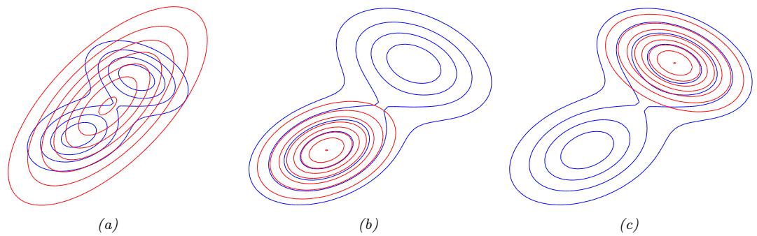
Figure 6.3: Illustrating forwards vs reverse KL on a bimodal distribution. The blue curves are the contours of the true distribution p. The red curves are the contours of the unimodal approximation q. (a) Minimizing forwards KL, DKL (p ′ q), wrt q causes q to “cover” p. (b-c) Minimizing reverse KL, DKL (q ′ p) wrt q causes q to “lock onto” one of the two modes of p. Adapted from Figure 10.3 of [Bis06]. Generated by KLfwdReverseMixGauss.ipynb.

We can gain an understanding of the optimal q by consider inputs x for which p(x)=0 but q(x) > 0. In this case, the term log q(x)/p(x) will be infinite. Thus minimizing the exclusive KL will force q to exclude all the areas of space for which p has zero probability. One way to do this is for q to put probability mass in very few parts of space; this is called zero-forcing or mode-seeking behavior. In this case, q will typically under-estimate the support of p. We illustrate mode seeking when p is bimodal but q is unimodal in Figure 6.3(b-c).

6.3 Mutual information *

The KL divergence gave us a way to measure how similar two distributions were. How should we measure how dependant two random variables are? One thing we could do is turn the question of measuring the dependence of two random variables into a question about the similarity of their distributions. This gives rise to the notion of mutual information (MI) between two random variables, which we define below.

6.3.1 Definition

The mutual information between rv’s X and Y is defined as follows:

\[\mathbb{E}\left(X;Y\right) \triangleq D\_{\text{KL}}\left(p(x,y) \parallel p(x)p(y)\right) = \sum\_{y \in Y} \sum\_{x \in X} p(x,y) \log \frac{p(x,y)}{p(x)\, p(y)}\tag{6.47}\]

(We write I(X; Y ) instead of I(X, Y ), in case X and/or Y represent sets of variables; for example, we can write I(X; Y,Z) to represent the MI between X and (Y,Z).) For continuous random variables, we just replace sums with integrals.

It is easy to see that MI is always non-negative, even for continuous random variables, since

\[\mathbb{E}\left(X;Y\right) = D\_{\text{KL}}\left(p(x,y) \parallel p(x)p(y)\right) \geq 0\tag{6.48}\]

We achieve the bound of 0 i! p(x, y) = p(x)p(y).

6.3.2 Interpretation

Knowing that the mutual information is a KL divergence between the joint and factored marginal distributions tells us that the MI measures the information gain if we update from a model that treats the two variables as independent p(x)p(y) to one that models their true joint density p(x, y).

To gain further insight into the meaning of MI, it helps to re-express it in terms of joint and conditional entropies, as follows:

\[\mathbb{E}(X;Y) = \mathbb{E}(X) - \mathbb{E}(X|Y) = \mathbb{E}(Y) - \mathbb{E}(Y|X) \tag{6.49}\]

Thus we can interpret the MI between X and Y as the reduction in uncertainty about X after observing Y , or, by symmetry, the reduction in uncertainty about Y after observing X. Incidentally, this result gives an alternative proof that conditioning, on average, reduces entropy. In particular, we have 0 ↘ I(X; Y ) = H (X) ↑ H (X|Y ), and hence H (X|Y ) ↘ H (X).

We can also obtain a di!erent interpretation. One can show that

\[\mathbb{H}(X;Y) = \mathbb{H}(X,Y) - \mathbb{H}(X|Y) - \mathbb{H}(Y|X) \tag{6.50}\]

Finally, one can show that

\[\mathbb{E}\left(X;Y\right) = \mathbb{E}\left(X\right) + \mathbb{E}\left(Y\right) - \mathbb{E}\left(X,Y\right) \tag{6.51}\]

See Figure 6.4 for a summary of these equations in terms of an information diagram. (Formally, this is a signed measure mapping set expressions to their information-theoretic counterparts [Yeu91].)

6.3.3 Example

As an example, let us reconsider the example concerning prime and even numbers from Section 6.1.3. Recall that H (X) = H (Y ) = 1. The conditional distribution p(Y |X) is given by normalizing each row:

\[ \begin{array}{c|ccc} & \mathbf{Y} = \mathbf{0} & \mathbf{Y} = \mathbf{1} \\ \hline \mathbf{X} = \mathbf{0} & \frac{1}{4} & \frac{3}{4} \\ \mathbf{X} = \mathbf{1} & \frac{3}{4} & \frac{1}{4} \end{array} \]

Hence the conditional entropy is

\[\mathbb{H}\left(Y|X\right) = -\left[\frac{1}{8}\log\_2\frac{1}{4} + \frac{3}{8}\log\_2\frac{3}{4} + \frac{3}{8}\log\_2\frac{3}{4} + \frac{1}{8}\log\_2\frac{1}{4}\right] = 0.81\text{ bits}\tag{6.52}\]

and the mutual information is

\[\mathbb{E}\left(X;Y\right) = \mathbb{E}\left(Y\right) - \mathbb{E}\left(Y|X\right) = \left(1 - 0.81\right)\text{ bits} = 0.19\text{ bits} \tag{6.53}\]

You can easily verify that

\[\mathbb{H}(X,Y) = \mathbb{H}(X|Y) + \mathbb{I}(X;Y) + \mathbb{H}(Y|X) \tag{6.54}\]

= (0.81 + 0.19 + 0.81) bits = 1.81 bits (6.55)

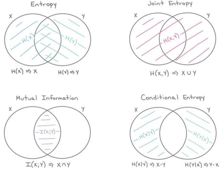
Figure 6.4: The marginal entropy, joint entropy, conditional entropy and mutual information represented as information diagrams. Used with kind permission of Katie Everett.

6.3.4 Conditional mutual information

We can define the conditional mutual information in the obvious way

\[\mathbb{E}\left(X;Y|Z\right) \stackrel{\Delta}{=} \mathbb{E}\_{p(Z)}\left[\mathbb{I}(X;Y)|Z\right] \tag{6.56}\]

\[\mathbb{E}\_x = \mathbb{E}\_{p(x,y,z)} \left[ \log \frac{p(x,y|z)}{p(x|z)p(y|z)} \right] \tag{6.57}\]

\[0 = \mathbb{H}\left(X|Z\right) + \mathbb{H}\left(Y|Z\right) - \mathbb{H}\left(X, Y|Z\right) \tag{6.58}\]

\[\mathbb{H} = \mathbb{H}\left(X|Z\right) - \mathbb{H}\left(X|Y, Z\right) = \mathbb{H}\left(Y|Z\right) - \mathbb{H}\left(Y|X, Z\right) \tag{6.59}\]

\[\mathcal{E} = \mathbb{H}\left(X, Z\right) + \mathbb{H}\left(Y, Z\right) - \mathbb{H}\left(Z\right) - \mathbb{H}\left(X, Y, Z\right) \tag{6.60}\]

\[\mathbf{x} = \mathbb{I}(Y; X, Z) - \mathbb{I}(Y; Z) \tag{6.61}\]

The last equation tells us that the conditional MI is the extra (residual) information that X tells us about Y , excluding what we already knew about Y given Z alone.

We can rewrite Equation (6.61) as follows:

\[\mathbb{I}(Z, Y; X) = \mathbb{I}(Z; X) + \mathbb{I}(Y; X | Z) \tag{6.62}\]

Generalizing to N variables, we get the chain rule for mutual information:

\[\mathbb{E}\left(Z\_1,\ldots,Z\_N;X\right) = \sum\_{n=1}^N \mathbb{I}\left(Z\_n;X\middle|Z\_1,\ldots,Z\_{n-1}\right) \tag{6.63}\]

6.3.5 MI as a “generalized correlation coe”cient”

Suppose that (x, y) are jointly Gaussian:

\[ \begin{pmatrix} x \\ y \end{pmatrix} \sim \mathcal{N} \left( \mathbf{0}, \begin{pmatrix} \sigma^2 & \rho \sigma^2 \\ \rho \sigma^2 & \sigma^2 \end{pmatrix} \right) \tag{6.64} \]

We now show how to compute the mutual information between X and Y .

Using Equation (6.26), we find that the entropy is

\[h(X,Y) = \frac{1}{2} \log \left[ (2\pi e)^2 \det \Sigma \right] = \frac{1}{2} \log \left[ (2\pi e)^2 \sigma^4 (1-\rho^2) \right] \tag{6.65}\]

Since X and Y are individually normal with variance ε², we have

\[h(X) = h(Y) = \frac{1}{2} \log \left[ 2\pi e \sigma^2 \right] \tag{6.66}\]

Hence

\[I(X,Y) = h(X) + h(Y) - h(X,Y) \tag{6.67}\]

\[=\log[2\pi e\sigma^2] - \frac{1}{2}\log[(2\pi e)^2\sigma^4(1-\rho^2)]\tag{6.68}\]

\[\dot{\rho} = \frac{1}{2} \log[(2\pi e\sigma^2)^2] - \frac{1}{2} \log[(2\pi e\sigma^2)^2(1-\rho^2)]\tag{6.69}\]

\[\dot{\rho} = \frac{1}{2} \log \frac{1}{1 - \rho^2} = -\frac{1}{2} \log[1 - \rho^2] \tag{6.70}\]

We now discuss some interesting special cases.

• 1. ς = 1. In this case, X = Y , and I(X, Y ) = ∈, which makes sense. Observing Y tells us an infinite amount of information about X (as we know its real value exactly).
• 2. ς = 0. In this case, X and Y are independent, and I(X, Y )=0, which makes sense. Observing Y tells us nothing about X.
• 3. ς = ↑1. In this case, X = ↑Y , and I(X, Y ) = ∈, which again makes sense. Observing Y allows us to predict X to infinite precision.

Now consider the case where X and Y are scalar, but not jointly Gaussian. In general it can be di”cult to compute the mutual information between continuous random variables, because we have to estimate the joint density p(X, Y ). For scalar variables, a simple approximation is to discretize or quantize them, by dividing the ranges of each variable into bins, and computing how many values fall in each histogram bin [Sco79]. We can then easily compute the MI using the empirical pmf.

Unfortunately, the number of bins used, and the location of the bin boundaries, can have a significant e!ect on the results. One way to avoid this is to use K-nearest neighbor distances to estimate densities in a non-parametric, adaptive way. This is the basis of the KSG estimator for MI proposed in [KSG04]. This is implemented in the sklearn.feature\_selection.mutual\_info\_regression function. For papers related to this estimator, see [GOV18; HN19].

6.3.6 Normalized mutual information

For some applications, it is useful to have a normalized measure of dependence, between 0 and 1. We now discuss one way to construct such a measure.

First, note that

\[\mathbb{E}\left(X;Y\right) = \mathbb{E}\left(X\right) - \mathbb{E}\left(X|Y\right) \le \mathbb{E}\left(X\right) \tag{6.71}\]

\[=\mathbb{H}\left(Y\right)-\mathbb{H}\left(Y|X\right)\leq\mathbb{H}\left(Y\right)\tag{6.72}\]

so

\[0 \le \mathbb{I}\left(X;Y\right) \le \min\left(\mathbb{H}\left(X\right), \mathbb{H}\left(Y\right)\right) \tag{6.73}\]

Therefore we can define the normalized mutual information as follows:

\[NMI(X,Y) = \frac{\mathbb{I}\left(X;Y\right)}{\min\left(\mathbb{H}\left(X\right), \mathbb{H}\left(Y\right)\right)} \le 1\tag{6.74}\]

This normalized mutual information ranges from 0 to 1. When NMI(X, Y )=0, we have I(X; Y )=0, so X and Y are independent. When NMI(X, Y )=1, and H (X) < H (Y ), we have

\[\mathbb{H}(X;Y) = \mathbb{H}(X) - \mathbb{H}(X|Y) = \mathbb{H}(X) \implies \mathbb{H}(X|Y) = 0 \tag{6.75}\]

and so X is a deterministic function of Y . For example, suppose X is a discrete random variable with pmf [0.5, 0.25, 0.25]. We have MI(X, X)=1.5 (using log base 2), and H(X)=1.5, so the normalized MI is 1, as is to be expected.

For continuous random variables, it is harder to normalize the mutual information, because of the need to estimate the di!erential entropy, which is sensitive to the level of quantization. See Section 6.3.7 for further discussion.

6.3.7 Maximal information coe”cient

As we discussed in Section 6.3.6, it is useful to have a normalized estimate of the mutual information, but this can be tricky to compute for real-valued data. One approach, known as the maximal information coe”cient (MIC) [Res+11], is to define the following quantity:

\[\text{MIC}(X, Y) = \max\_{G} \frac{\mathbb{I}((X, Y)|\_{G})}{\log ||G||} \tag{6.76}\]

where G is the set of 2d grids, and (X, Y )|^G represents a discretization of the variables onto this grid, and ||G|| is min(Gx, Gy), where G^x is the number of grid cells in the x direction, and G^y is the number of grid cells in the y direction. (The maximum grid resolution depends on the sample size ⁿ; they suggest restricting grids so that ^GxG^y ↘ ^B(n), where ^B(n) = ⁿ↽, where ^ϱ = 0.6.) The denominator is the entropy of a uniform joint distribution; dividing by this ensures 0 ↘ MIC ↘ 1.

The intuition behind this statistic is the following: if there is a relationship between X and Y , then there should be some discrete gridding of the 2d input space that captures this. Since we don’t know the correct grid to use, MIC searches over di!erent grid resolutions (e.g., 2x2, 2x3, etc), as well as over locations of the grid boundaries. Given a grid, it is easy to quantize the data and compute

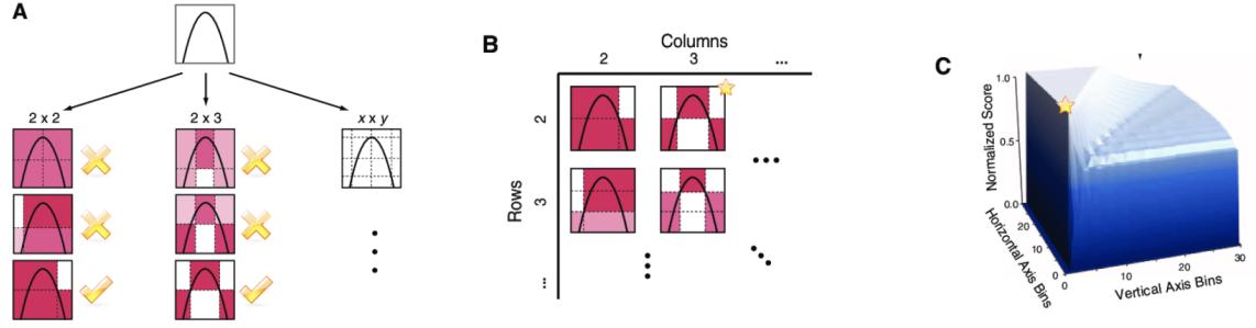
Figure 6.5: Illustration of how the maximal information coe”cient (MIC) is computed. (a) We search over di!erent grid resolutions, and grid cell locations, and compute the MI for each. (b) For each grid resolution (k, l), we define set M(k, l) to be the maximum MI for any grid of that size, normalized by log(min(k, l)). (c) We visualize the matrix M. The maximum entry (denoted by a star) is defined to be the MIC. From Figure 1 of [Res+11]. Used with kind permission of David Reshef.

1001. We define the characteristic matrix M(k,l) to be the maximum MI achievable by any grid of size (k,l), normalized by log(min(k,l)). The MIC is then the maximum entry in this matrix, maxkl⇑B(n) M(k,l). See Figure 6.5 for a visualization of this process.

In [Res+11], they show that this quantity exhibits a property known as equitability, which means that it gives similar scores to equally noisy relationships, regardless of the type of relationship (e.g., linear, non-linear, non-functional).

In [Res+16], they present an improved estimator, called MICe, which is more e”cient to compute, and only requires optimizing over 1d grids, which can be done in O(n) time using dynamic programming. They also present another quantity, called TICe (total information content), that has higher power to detect relationships from small sample sizes, but lower equitability. This is defined to be $ kl⇑B(n) ^M(k,l). They recommend using TICe to screen a large number of candidate relationships, and then using MICe to quantify the strength of the relationship. For an e”cient implementation of both of these metrics, see [Alb+18].

We can interpret MIC of 0 to mean there is no relationship between the variables, and 1 to represent a noise-free relationship of any form. This is illustrated in Figure 6.6. Unlike correlation coe”cients, MIC is not restricted to finding linear relationships. For this reason, the MIC has been called “a correlation for the 21st century” [Spe11].

In Figure 6.7, we give a more interesting example, from [Res+11]. The data consists of 357 variables measuring a variety of social, economic, health and political indicators, collected by the World Health Organization (WHO). On the left of the figure, we see the correlation coe”cient (CC) plotted against the MIC for all 63,546 variable pairs. On the right of the figure, we see scatter plots for particular pairs of variables, which we now discuss:

• The point marked C (near 0,0 on the plot) has a low CC and a low MIC. The corresponding scatter plot makes it clear that there is no relationship between these two variables (percentage of lives lost to injury and density of dentists in the population).
• The points marked D and H have high CC (in absolute value) and high MIC, because they

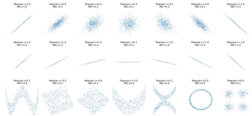
Figure 6.6: Plots of some 2d distributions and the corresponding estimate of correlation coe”cient R² and the maximal information coe”cient (MIC). Compare to Figure 3.1. Generated by MIC\_correlation\_2d.ipynb.

represent nearly linear relationships.

• The points marked E, F, and G have low CC but high MIC. This is because they correspond to non-linear (and sometimes, as in the case of E and F, non-functional, i.e., one-to-many) relationships between the variables.

6.3.8 Data processing inequality

Suppose we have an unknown variable X, and we observe a noisy function of it, call it Y . If we process the noisy observations in some way to create a new variable Z, it should be intuitively obvious that we cannot increase the amount of information we have about the unknown quantity, X. This is known as the data processing inequality. We now state this more formally, and then prove it.

Theorem 6.3.1. Suppose X ↔︎ Y ↔︎ Z forms a Markov chain, so that X ⇔ Z|Y . Then I(X; Y ) ∋ I(X;Z).

Proof. By the chain rule for mutual information (Equation (6.62)), we can expand the mutual information in two di!erent ways:

\[\mathbb{I}\left(X;Y,Z\right) = \mathbb{I}\left(X;Z\right) + \mathbb{I}\left(X;Y|Z\right) \tag{6.77}\]

\[=\mathbb{I}\left(X;Y\right) + \mathbb{I}\left(X;Z|Y\right) \tag{6.78}\]

Since X ⇔ Z|Y , we have I(X;Z|Y )=0, so

\[\mathbb{I}\left(X;Z\right) + \mathbb{I}\left(X;Y|Z\right) = \mathbb{I}\left(X;Y\right) \tag{6.79}\]

Since I(X; Y |Z) ∋ 0, we have I(X; Y ) ∋ I(X;Z). Similarly one can prove that I(Y ;Z) ∋ I(X;Z).

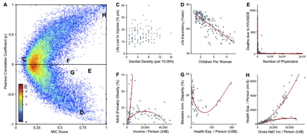
Figure 6.7: Left: Correlation coe”cient vs maximal information criterion (MIC) for all pairwise relationships in the WHO data. Right: scatter plots of certain pairs of variables. The red lines are non-parametric smoothing regressions fit separately to each trend. From Figure 4 of [Res+11]. Used with kind permission of David Reshef.

6.3.9 Su”cient Statistics

An important consequence of the DPI is the following. Suppose we have the chain ϖ ↔︎ D ↔︎ s(D). Then

\[\mathbb{1}\left(\theta; s(\mathcal{D})\right) \le \mathbb{1}\left(\theta; \mathcal{D}\right) \tag{6.80}\]

If this holds with equality, then we say that s(D) is a su!cient statistic of the data D for the purposes of inferring ϖ. In this case, we can equivalently write ϖ ↔︎ s(D) ↔︎ D, since we can reconstruct the data from knowing s(D) just as accurately as from knowing ϖ.

An example of a su”cient statistic is the data itself, s(D) = D, but this is not very useful, since it doesn’t summarize the data at all. Hence we define a minimal su!cient statistic s(D) as one which is su”cient, and which contains no extra information about ϖ; thus s(D) maximally compresses the data D without losing information which is relevant to predicting ϖ. More formally, we say s is a minimal su”cient statistic for D if for all su”cient statistics s↗ (D) there is some function f such that s(D) = f(s↗ (D)). We can summarize the situation as follows:

\[ \theta \to s(\mathcal{D}) \to s'(\mathcal{D}) \to \mathcal{D} \tag{6.81} \]

Here s↗ (D) takes s(D) and adds redundant information to it, thus creating a one-to-many mapping.

$ For example, a minimal su”cient statistic for a set of N Bernoulli trials is simply N and N¹ = ⁿ I(Xⁿ = 1), i.e., the number of successes. In other words, we don’t need to keep track of the entire sequence of heads and tails and their ordering, we only need to keep track of the total number of heads and tails. Similarly, for inferring the mean of a Gaussian distribution with known variance we only need to know the empirical mean and number of samples.

6.3.10 Fano’s inequality *

A common method for feature selection is to pick input features X^d which have high mutual information with the response variable Y . Below we justify why this is a reasonable thing to do. In particular, we state a result, known as Fano’s inequality, which bounds the probability of misclassification (for any method) in terms of the mutual information between the features X and the class label Y .

Theorem 6.3.2. (Fano’s inequality) Consider an estimator ^{Yˆ = f}(X) such that ^{Y ↔︎ X ↔︎ Yˆ} forms a Markov chain. Let ^E be the event ^Yˆ ↗^{= Y} , indicating that an error occured, and let ^{Pe = P}(^Y ↗^{= Yˆ} ) be the probability of error. Then we have

\[\mathbb{H}\left(Y|X\right) \le \mathbb{H}\left(Y|\hat{Y}\right) \le \mathbb{H}\left(E\right) + P\_e \log |\mathcal{Y}|\tag{6.82}\]

Since H (E) ↘ 1, as we saw in Figure 6.1, we can weaken this result to get

\[1 + P\_e \log |\mathcal{Y}| \ge \mathbb{H} \left( Y | X \right) \tag{6.83}\]

and hence

\[P\_e \ge \frac{\mathbb{H}(Y|X) - 1}{\log|\mathcal{Y}|} \tag{6.84}\]

Thus minimizing H (Y |X) (which can be done by maximizing I(X; Y )) will also minimize the lower bound on Pe.

Proof. (From [CT06, p38].) Using the chain rule for entropy, we have

\[\mathbb{H}\left(E,Y|\hat{Y}\right) = \mathbb{H}\left(Y|\hat{Y}\right) + \underbrace{\mathbb{H}\left(E|Y,\hat{Y}\right)}\_{=0} \tag{6.85}\]

\[=\mathbb{H}\left(E|\hat{Y}\right) + \mathbb{H}\left(\check{Y}|E,\hat{Y}\right) \tag{6.86}\]

Since conditioning reduces entropy (see Section 6.2.4), we have H ^E|Y^ˆ ↘ H (E). The final term can be bounded as follows:

\[\mathbb{H}\left(Y|E,\hat{Y}\right) = P(E=0)\,\mathbb{H}\left(Y|\hat{Y},E=0\right) + P(E=1)\,\mathbb{H}\left(Y|\hat{Y},E=1\right) \tag{6.87}\]

\[\leq (1 - P\_e)0 + P\_e \log |\mathcal{Y}|\tag{6.88}\]

Hence

\[\mathbb{H}\left(Y|\hat{Y}\right) \le \underbrace{\mathbb{H}\left(E|\hat{Y}\right)}\_{\le \mathbb{H}(E)} + \underbrace{\mathbb{H}\left(Y|E,\hat{Y}\right)}\_{P\_e \log|\mathcal{Y}|} \tag{6.89}\]

Finally, by the data processing inequality, we have ^I(^Y ; ^Yˆ ) ↘ ^I(^Y ; ^X), so ^H (^{Y |}X) ↘ ^{H Y |}Y^ˆ , which establishes Equation (6.82).

6.4 Exercises

Exercise 6.1 [Expressing mutual information in terms of entropies † ] Prove the following identities:

\[H(X;Y) = H(X) - H(X|Y) = H(Y) - H(Y|X) \tag{6.90}\]

and

\[H(X,Y) = H(X|Y) + H(Y|X) + I(X;Y) \tag{6.91}\]

Exercise 6.2 [Relationship between ^D(p||q) and ^χ2 statistic]

(Source: [CT91, Q12.2].)

Show that, if p(x) ∞ q(x), then

\[D\_{\rm KL} \left( p \parallel q \right) \approx \frac{1}{2} \chi^2 \tag{6.92}\]

where

\[\chi^2 = \sum\_{x} \frac{(p(x) - q(x))^2}{q(x)} \tag{6.93}\]

Hint: write

p(x) = #(x) + q(x) (6.94)

\[\frac{p(x)}{q(x)} = 1 + \frac{\Delta(x)}{q(x)}\tag{6.95}\]

and use the Taylor series expansion for log(1 + x).

\[\log(1+x) = x - \frac{x^2}{2} + \frac{x^3}{3} - \frac{x^4}{4} \cdots \tag{6.96}\]

for ↑1 < x ↗ 1.

Exercise 6.3 [Fun with entropies † ]

(Source: Mackay.)

Consider the joint distribution p(X, Y )

			x
		1	2	3	4
	1	1/8	1/16	1/32	1/32
y	2	1/16	1/8	1/32	1/32
	3	1/16	1/16	1/16	1/16
	4	1/4	0	0	0

• 1. What is the joint entropy H(X, Y )?
• 2. What are the marginal entropies H(X) and H(Y )?
• 3. The entropy of X conditioned on a specific value of y is defined as

\[H(X|Y=y) = -\sum\_{x} p(x|y) \log p(x|y) \tag{6.97}\]

Compute H(X|y) for each value of y. Does the posterior entropy on X ever increase given an observation of Y ?

4. The conditional entropy is defined as

\[H(X|Y) = \sum\_{y} p(y)H(X|Y=y) \tag{6.98}\]

Compute this. Does the posterior entropy on X increase or decrease when averaged over the possible values of Y ?

5. What is the mutual information between X and Y ?

Exercise 6.4 [Forwards vs reverse KL divergence]

(Source: Exercise 33.7 of [Mac03].) Consider a factored approximation q(x, y) = q(x)q(y) to a joint distribution p(x, y). Show that to minimize the forwards KL DKL (p ′ q) we should set q(x) = p(x) and q(y) = p(y), i.e., the optimal approximation is a product of marginals.

Now consider the following joint distribution, where the rows represent y and the columns x.

	1	2	3	4
1	1/8	1/8	0	0
2	1/8	1/8	0	0
3	0	0	1/4	0
4	0	0	0	1/4

Show that the reverse KL DKL (q ′ p) for this p has three distinct minima. Identify those minima and evaluate DKL (q ′ p) at each of them. What is the value of DKL (q ′ p) if we set q(x, y) = p(x)p(y)?

7 Linear Algebra

This chapter is co-authored with Zico Kolter.

7.1 Introduction

Linear algebra is the study of matrices and vectors. In this chapter, we summarize the key material that we will need throughout the book. Much more information can be found in other sources, such as [Str09; Ips09; Kle13; Mol04; TB97; Axl15; Tho17; Agg20; LLM14].

7.1.1 Notation

In this section, we define some notation.

7.1.1.1 Vectors

^A vector ^{x → Rn} is a list of ⁿ numbers, usually written as a column vector

\[\begin{array}{c} \begin{bmatrix} x\_1\\x\_2\\\vdots\\\vdots\\x\_n \end{bmatrix} . \end{array} . \tag{7.1}\]

The vector of all ones is denoted 1. The vector of all zeros is denoted 0. The unit vector eⁱ is a vector of all 0’s, except entry i, which has value 1:

\[\mathbf{e}\_i = (0, \dots, 0, 1, 0, \dots, 0)\tag{7.2}\]

This is also called a one-hot vector.

7.1.1.2 Matrices

^A matrix ^{A → Rm}↔︎ⁿ with ^m rows and ⁿ columns is a 2d array of numbers, arranged as follows:

\[\mathbf{A} = \begin{bmatrix} a\_{11} & a\_{12} & \cdots & a\_{1n} \\ a\_{21} & a\_{22} & \cdots & a\_{2n} \\ \vdots & \vdots & \ddots & \vdots \\ a\_{m1} & a\_{m2} & \cdots & a\_{mn} \end{bmatrix} \tag{7.3}\]

If m = n, the matrix is said to be square.

We use the notation Aij or Ai,j to denote the entry of A in the ith row and jth column. We use the notation Ai,: to denote the i’th row and A:,j to denote the j’th column. We treat all vectors as column vectors by default (so Ai,: is viewed as a column vector with n entries). We use bold upper case letters to denote matrices, bold lower case letters to denote vectors, and non-bold letters to denote scalars.

We can view a matrix as a set of columns stacked along the horizontal axis:

\[\mathbf{A} = \begin{bmatrix} | & | & & | \\ \mathbf{A}\_{:,1} & \mathbf{A}\_{:,2} & \cdots & \mathbf{A}\_{:,n} \\ | & | & & | \end{bmatrix} . \tag{7.4}\]

For brevity, we will denote this by

\[\mathbf{A} = [\mathbf{A}\_{:,1}, \mathbf{A}\_{:,2}, \dots, \mathbf{A}\_{:,n}] \tag{7.5}\]

We can also view a matrix as a set of rows stacked along the vertical axis:

\[\mathbf{A} = \begin{bmatrix} \cdots & \mathbf{A}\_{1:}^{\mathrm{T}} & \cdots \\ \cdots & \mathbf{A}\_{2:}^{\mathrm{T}} & \cdots \\ & \vdots & \\ \cdots & \mathbf{A}\_{m:}^{\mathrm{T}} & \cdots \end{bmatrix}. \tag{7.6}\]

For brevity, we will denote this by

\[\mathbf{A} = [\mathbf{A}\_{1,:}; \mathbf{A}\_{2,:}; \dots; \mathbf{A}\_{m,:}] \tag{7.7}\]

(Note the use of a semicolon.)

The transpose of a matrix results from “flipping” the rows and columns. Given a matrix ^{A → Rm}↔︎n, its transpose, written ^{AT → Rn}↔︎^m, is defined as

\[(\mathbf{A}^{\mathsf{T}})\_{ij} = A\_{ji} \tag{7.8}\]

The following properties of transposes are easily verified:

\[(\mathbf{A}^{\mathsf{T}})^{\mathsf{T}} = \mathbf{A} \tag{7.9}\]

\[(\mathbf{A}\mathbf{B})^{\mathsf{T}} = \mathbf{B}^{\mathsf{T}}\mathbf{A}^{\mathsf{T}} \tag{7.10}\]

\[(\mathbf{A} + \mathbf{B})^{\mathsf{T}} = \mathbf{A}^{\mathsf{T}} + \mathbf{B}^{\mathsf{T}} \tag{7.11}\]

If a square matrix satisfies A = A^T, it is called symmetric. We denote the set of all symmetric matrices of size n as Sⁿ.

7.1.1.3 Tensors

A tensor (in machine learning terminology) is just a generalization of a 2d array to more than 2 dimensions, as illustrated in Figure 7.1. For example, the entries of a 3d tensor are denoted by Aijk.

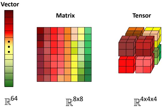
Figure 7.1: Illustration of a 1d vector, 2d matrix, and 3d tensor. The colors are used to represent individual entries of the vector; this list of numbers can also be stored in a 2d matrix, as shown. (In this example, the matrix is layed out in column-major order, which is the opposite of that used by Python.) We can also reshape the vector into a 3d tensor, as shown.

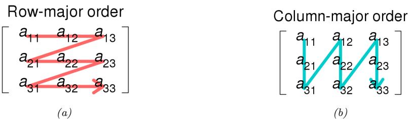
Figure 7.2: Illustration of (a) row-major vs (b) column-major order. From https: // commons. wikimedia. org/ wiki/ File: Row\_ and\_ column\_ major\_ order. svg . Used with kind permission of Wikipedia author Cmglee.

The number of dimensions is known as the order or rank of the tensor.1 In mathematics, tensors can be viewed as a way to define multilinear maps, just as matrices can be used to define linear functions, although we will not need to use this interpretation.

We can reshape a matrix into a vector by stacking its columns on top of each other, as shown in Figure 7.1. This is denoted by

\[\text{vec}(\mathbf{A}) = [\mathbf{A}\_{:,1}; \cdots; \mathbf{A}\_{:,n}] \in \mathbb{R}^{mn \times 1} \tag{7.12}\]

Conversely, we can reshape a vector into a matrix. There are two choices for how to do this, known as row-major order (used by languages such as Python and C++) and column-major order (used by languages such as Julia, Matlab, R and Fortran). See Figure 7.2 for an illustration of the di!erence.

^1. Note, however, that the rank of a 2d matrix is a di!erent concept, as discussed in Section 7.1.4.3.

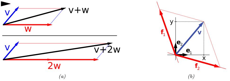
Figure 7.3: (a) Top: A vector v (blue) is added to another vector w (red). Bottom: w is stretched by a factor of 2, yielding the sum v + 2w. From https: // en. wikipedia. org/ wiki/ Vector\_ space . Used with kind permission of Wikipedia author IkamusumeFan (b) A vector v in R² (blue) expressed in terms of di!erent bases: using the standard basis of R², v = xe¹ + ye² (black), and using a di!erent, non-orthogonal basis: v = f¹ + f² (red). From https: // en. wikipedia. org/ wiki/ Vector\_ space . Used with kind permission of Wikiepdia author Jakob.scholbach.

7.1.2 Vector spaces

In this section, we discuss some fundamental concepts in linear algebra.

7.1.2.1 Vector addition and scaling

We can view a vector ^{x → Rn} as defining a point in ⁿ-dimensional Euclidean space. A vector space is a collection of such vectors, which can be added together, and scaled by scalars (1-dimensional numbers), in order to create new points. These operations are defined to operate elementwise, in the obvious way, namely x + y = (x¹ + y1,…,xⁿ + yn) and cx = (cx1, . . . , cxn), where c → R. See Figure 7.3a for an illustration.

7.1.2.2 Linear independence, spans and basis sets

A set of vectors {x1, x2,… xn} is said to be (linearly) independent if no vector can be represented as a linear combination of the remaining vectors. Conversely, a vector which can be represented as a linear combination of the remaining vectors is said to be (linearly) dependent. For example, if

\[x\_n = \sum\_{i=1}^{n-1} \alpha\_i x\_i \tag{7.13}\]

for some {ϱ1,…, ϱⁿ→¹} then xⁿ is dependent on {x1,…, xⁿ→¹}; otherwise, it is independent of {x1,…, xⁿ→¹}.

The span of a set of vectors {x1, x2,…, xn} is the set of all vectors that can be expressed as a linear combination of {x1,…, xn}. That is,

\[\text{span}(\{x\_1, \ldots, x\_n\}) \stackrel{\Delta}{=} \left\{ \mathbf{v} : \mathbf{v} = \sum\_{i=1}^n \alpha\_i x\_i, \ \alpha\_i \in \mathbb{R} \right\}.\tag{7.14}\]

It can be shown that if {x1,…, ^xn} is a set of ⁿ linearly independent vectors, where each ^{xi → R}n, then span({x1,…, ^xn}) = ^Rn. In other words, any vector ^{v → Rn} can be written as a linear combination of x¹ through xn.

A basis B is a set of linearly independent vectors that spans the whole space, meaning that span(B) = ^Rn. There are often multiple bases to choose from, as illustrated in Figure 7.3b. The standard basis uses the coordinate vectors e¹ = (1, 0,…, 0), up to eⁿ = (0, 0,…, 0, 1). This lets us translate back and forth between viewing a vector in R² as an either an “arrow in the plane”, rooted at the origin, or as an ordered list of numbers (corresponding to the coe”cients for each basis vector).

7.1.2.3 Linear maps and matrices

A linear map or linear transformation is any function f : V ↔︎ W such that f(v+w) = f(v)+f(w) and f(a v) = a f(v) for all v, w → V. Once the basis of V is chosen, a linear map f : V ↔︎ W is completely determined by specifying the images of the basis vectors, because any element of V can be expressed uniquely as a linear combination of them.

Suppose ^V = ^Rn and ^W = ^Rm. We can compute ^f(vi) ^{→ Rm} for each basis vector in ^V, and store these along the columns of an ^{m ↓ n} matrix ^A. We can then compute ^{y = f}(x) ^{→ Rm} for any ^{x → Rn} as follows:

\[y = \left(\sum\_{j=1}^{n} a\_{1j} x\_j, \dots, \sum\_{j=1}^{n} a\_{mj} x\_j\right) \tag{7.15}\]

This corresponds to multiplying the vector x by the matrix A:

\[y = \mathbf{A}x\tag{7.16}\]

See Section 7.2 for more details.

If the function is invertible, we can write

\[x = \mathbf{A}^{-1}y\tag{7.17}\]

See Section 7.3 for details.

7.1.2.4 Range and nullspace of a matrix

Suppose we view a matrix ^{A → Rm}↔︎ⁿ as a set of ⁿ vectors in ^Rm. The range (sometimes also called the column space) of this matrix is the span of the columns of A. In other words,

\[\text{range}(\mathbf{A}) \triangleq \{ \mathbf{v} \in \mathbb{R}^{m} : \mathbf{v} = \mathbf{A}x, x \in \mathbb{R}^{n} \}. \tag{7.18}\]

This can be thought of as the set of vectors that can be “reached” or “generated” by A; it is a subspace of R^m whose dimensionality is given by the rank of A (see Section 7.1.4.3). The nullspace of a matrix ^{A → Rm}↔︎ⁿ is the set of all vectors that get mapped to the null vector when multiplied by ^A, i.e.,

\[\text{nullspace}(\mathbf{A}) \triangleq \{ \mathbf{x} \in \mathbb{R}^n : \mathbf{A}\mathbf{x} = \mathbf{0} \}. \tag{7.19}\]

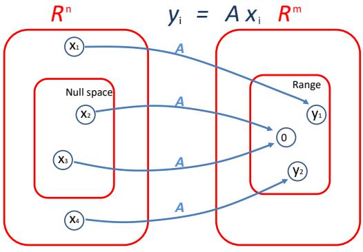
Figure 7.4: Visualization of the nullspace and range of an m → n matrix A. Here y¹ = Ax¹ and y² = Ax4, so y¹ and y² are in the range of A (are reachable from some x). Also Ax² = 0 and Ax³ = 0, so x² and x³ are in the nullspace of A (get mapped to 0). We see that the range is often a subset of the input domain of the mapping.

The span of the rows of A is the complement to the nullspace of A.

See Figure 7.4 for an illustration of the range and nullspace of a matrix. We shall discuss how to compute the range and nullspace of a matrix numerically in Section 7.5.4 below.

7.1.2.5 Linear projection

The projection of a vector ^{y → Rm} onto the span of {x1,…, ^xn} (here we assume ^{xi → Rm}) is the vector v → span({x1,…, xn}) , such that v is as close as possible to y, as measured by the Euclidean norm 7v ↑ y72. We denote the projection as Proj(y; {x1,…, xn}) and can define it formally as

\[\operatorname{Proj}(y; \{x\_1, \ldots, x\_n\}) = \operatorname{argmin}\_{\boldsymbol{\sigma} \in \operatorname{span}(\{\boldsymbol{\pi}\_1, \ldots, \boldsymbol{\pi}\_n\})} \|y - \boldsymbol{\sigma}\|\_2. \tag{7.20}\]

Given a (full rank) matrix ^{A → Rm}↔︎ⁿ with ^{m ∋ n}, we can define the projection of a vector ^{y → Rm} onto the range of A as follows:

\[\text{Proj}(\boldsymbol{y}; \mathbf{A}) = \text{argmin}\_{\boldsymbol{v} \in \mathcal{R}(\mathbf{A})} \|\boldsymbol{v} - \boldsymbol{y}\|\_{2} = \mathbf{A}(\mathbf{A}^{\mathsf{T}}\mathbf{A})^{-1}\mathbf{A}^{\mathsf{T}}\boldsymbol{y} \;. \tag{7.21}\]

These are the same as the normal equations from Section 11.2.2.2.

7.1.3 Norms of a vector and matrix

In this section, we discuss ways of measuring the “size” of a vector and matrix.

7.1.3.1 Vector norms

A norm of a vector 7x7 is, informally, a measure of the “length” of the vector. More formally, a norm is any function ^f : ^{Rn ↔︎ R} that satisfies 4 properties:

• For all ^{x → Rn}, ^f(x) ^{∋ 0} (non-negativity).

• f(x)=0 if and only if x = 0 (definiteness).
• For all ^{x → R}n, ^{t → R}, ^f(tx) = ^|t|f(x) (absolute value homogeneity).
• For all ^x, ^{y → R}n, ^f(^{x + y}) ↘ ^f(x) + ^f(y) (triangle inequality).

Consider the following common examples:

p-norm ⁷x7^p = ($^{n i}=1 |xi| p) ¹/p, for ^{p ∋ 1}.

2-norm ⁷x7^{2 =} -$^{n i}=1 x^{2 i} , also called Euclidean norm. Note that ⁷x7^{2 2} = x^Tx.

1-norm ⁷x7^{1 =} $^{n i}=1 |xi|.

Max-norm 7x7↘ = maxi|xi|.

0-norm ⁷x7^{0 =} $^{n i}=1 I(|xi| > 0). This is a pseudo norm, since it does not satisfy homogeneity. It counts the number of non-zero elements in x. If we define 0⁰ = 0, we can write this as ⁷x7^{0 =} $^{n i}=1 x⁰ i .

7.1.3.2 Matrix norms

Suppose we think of a matrix A ^{→ Rm}↔︎ⁿ as defining a linear function ^f(x) = Ax. We define the induced norm of A as the maximum amount by which f can lengthen any unit-norm input:

\[||\mathbf{A}||\_p = \max\_{\mathbf{x} \neq \mathbf{0}} \frac{||\mathbf{A}\mathbf{x}||\_p}{||\mathbf{x}||\_p} = \max\_{||\mathbf{x}|| = 1} ||\mathbf{A}\mathbf{x}||\_p \tag{7.22}\]

Typically p = 2, in which case

\[||\mathbf{A}||\_2 = \sqrt{\lambda\_{\text{max}}(\mathbf{A}^\mathsf{T}\mathbf{A})} = \max\_i \sigma\_i \tag{7.23}\]

where φmax(M) is the largest eigenvalue of M, and εⁱ is the i’th singular value.

The nuclear norm, also called the trace norm, is defined as

\[||\mathbf{A}||\_{\*} = \text{tr}(\sqrt{\mathbf{A}^{\mathsf{T}}\mathbf{A}}) = \sum\_{i} \sigma\_{i} \tag{7.24}\]

where ^≃ A^TA is the matrix square root. Since the singular values are always non-negative, we have

\[||\mathbf{A}||\_\* = \sum\_i |\sigma\_i| = ||\sigma||\_1 \tag{7.25}\]

Using this as a regularizer encourages many singular values to become zero, resulting in a low rank matrix. More generally, we can define the Schatten p-norm as

\[||\mathbf{A}||\_p = \left(\sum\_i \sigma\_i^p(\mathbf{A})\right)^{1/p} \tag{7.26}\]

If we think of a matrix as a vector, we can define the matrix norm in terms of a vector norm, ||A|| = ||vec(A)||. If the vector norm is the 2-norm, the corresponding matrix norm is the Frobenius norm:

\[||\mathbf{A}||\_F = \sqrt{\sum\_{i=1}^{m} \sum\_{j=1}^{n} a\_{ij}^2} = \sqrt{\text{tr}(\mathbf{A}^\mathsf{T} \mathbf{A})} = ||\text{vec}(\mathbf{A})||\_2 \tag{7.27}\]

If A is expensive to evaluate, but Av is cheap (for a random vector v), we can create a stochastic approximation to the Frobenius norm by using the Hutchinson trace estimator from Equation (7.37) as follows:

\[\mathbb{E}\left\|\mathbf{A}\right\|\_{F}^{2} = \text{tr}(\mathbf{A}^{\mathsf{T}}\mathbf{A}) = \mathbb{E}\left[\mathbf{v}^{\mathsf{T}}\mathbf{A}^{\mathsf{T}}\mathbf{A}\mathbf{v}\right] = \mathbb{E}\left[||\mathbf{A}\mathbf{v}||\_{2}^{2}\right] \tag{7.28}\]

where v ⇒ N (0, I).

7.1.4 Properties of a matrix

In this section, we discuss various scalar properties of matrices.

7.1.4.1 Trace of a square matrix

The trace of a square matrix A ^{→ Rn}↔︎ⁿ, denoted tr(A), is the sum of diagonal elements in the matrix:

\[\text{tr}(\mathbf{A}) \triangleq \sum\_{i=1}^{n} A\_{ii}. \tag{7.29}\]

The trace has the following properties, where ^{c → R} is a scalar, and A, B ^{→ Rn}↔︎ⁿ are square matrices:

\[\text{tr}(\mathbf{A}) = \text{tr}(\mathbf{A}^\top) \tag{7.30}\]

\[\text{tr}(\mathbf{A} + \mathbf{B}) = \text{tr}(\mathbf{A}) + \text{tr}(\mathbf{B})\tag{7.31}\]

\[\operatorname{tr}(c\mathbf{A}) = c\operatorname{tr}(\mathbf{A})\tag{7.32}\]

\[\text{tr}(\mathbf{AB}) = \text{tr}(\mathbf{BA})\tag{7.33}\]

\[\text{tr}(\mathbf{A}) = \sum\_{i=1}^{n} \lambda\_i \text{ where } \lambda\_i \text{ are the eigenvalues of } \mathbf{A} \tag{7.34}\]

We also have the following important cyclic permutation property: For A, B, C such that ABC is square,

\[\text{tr}(\mathbf{A}\mathbf{B}\mathbf{C}) = \text{tr}(\mathbf{B}\mathbf{C}\mathbf{A}) = \text{tr}(\mathbf{C}\mathbf{A}\mathbf{B})\tag{7.35}\]

From this, we can derive the trace trick, which rewrites the scalar inner product x^TAx as follows

\[\mathbf{x}^{\mathsf{T}}\mathbf{A}x = \text{tr}(\mathbf{x}^{\mathsf{T}}\mathbf{A}x) = \text{tr}(x\mathbf{x}^{\mathsf{T}}\mathbf{A})\tag{7.36}\]

In some cases, it may be expensive to evaluate the matrix A, but we may be able to cheaply evaluate matrix-vector products Av. Suppose v is a random vector such that E + vvT, = I. In this case, we can create a Monte Carlo approximation to tr(A) using the following identity:

\[\operatorname{tr}(\mathbf{A}) = \operatorname{tr}(\mathbf{A}\mathbb{E}\left[\mathbf{v}\mathbf{v}^{\mathsf{T}}\right]) = \operatorname{E}\left[\operatorname{tr}(\mathbf{A}\mathbf{v}\mathbf{v}^{\mathsf{T}})\right] = \operatorname{E}\left[\operatorname{tr}(\mathbf{v}^{\mathsf{T}}\mathbf{A}\mathbf{v})\right] = \operatorname{E}\left[\mathbf{v}^{\mathsf{T}}\mathbf{A}\mathbf{v}\right] \tag{7.37}\]

This is called the Hutchinson trace estimator [Hut90].

7.1.4.2 Determinant of a square matrix

The determinant of a square matrix, denoted det(A) or |A|, is a measure of how much it changes a unit volume when viewed as a linear transformation. (The formal definition is rather complex and is not needed here.)

The determinant operator satisfies these properties, where ^A, ^{B → Rn}↔︎ⁿ

\[|\mathbf{A}| = |\mathbf{A}^{\mathsf{T}}|\tag{7.38}\]

\[c|c\mathbf{A}| = c^n|\mathbf{A}|\tag{7.39}\]

\[|\mathbf{AB}| = |\mathbf{A}||\mathbf{B}|\tag{7.40}\]

\[|\mathbf{A}| = 0 \text{ iff } \mathbf{A} \text{ is singular} \tag{7.41}\]

\[|\mathbf{A}^{-1}| = 1/|\mathbf{A}| \text{ if } \mathbf{A} \text{ is not singular} \tag{7.42}\]

\[|\mathbf{A}| = \prod\_{i=1}^{n} \lambda\_i \text{ where } \lambda\_i \text{ are the eigenvalues of } \mathbf{A} \tag{7.43}\]

For a positive definite matrix A, we can write A = LLT, where L is the lower triangular Cholesky decomposition. In this case, we have

\[\det(\mathbf{A}) = \det(\mathbf{L}) \det(\mathbf{L}^{\mathsf{T}}) = \det(\mathbf{L})^2 \tag{7.44}\]

so

\[\log \det(\mathbf{A}) = 2 \log \det(\mathbf{L}) = 2 \log \prod\_{i} L\_{ii} = 2 \text{tr}(\log(\text{diag}(\mathbf{L}))) \tag{7.45}\]

7.1.4.3 Rank of a matrix

The column rank of a matrix A is the dimension of the space spanned by its columns, and the row rank is the dimension of the space spanned by its rows. It is a basic fact of linear algebra (that can be shown using the SVD, discussed in Section 7.5) that for any matrix A, columnrank(A) = rowrank(A), and so this quantity is simply referred to as the rank of A, denoted as rank(A). The following are some basic properties of the rank:

• For A ^{→ Rm}↔︎ⁿ, rank(A) ↘ min(m, n). If rank(A) = min(m, n), then A is said to be full rank, otherwise it is called rank deficient.
• For ^{A → Rm}↔︎ⁿ, rank(A) = rank(A^T) = rank(A^TA) = rank(AA^T).
• For ^{A → Rm}↔︎ⁿ, ^{B → Rn}↔︎^p, rank(AB) ↘ min(rank(A),rank(B)).

• For ^A, ^{B → R}m↔︎n, rank(^{A + B}) ↘ rank(A) + rank(B).

One can show that a square matrix is invertible i! it is full rank.

7.1.4.4 Condition numbers

The condition number of a matrix A is a measure of how numerically stable any computations involving A will be. It is defined as follows:

\[\kappa(\mathbf{A}) \stackrel{\Delta}{=} ||\mathbf{A}|| \cdot ||\mathbf{A}^{-1}||\tag{7.46}\]

where ||A|| is the norm of the matrix. We can show that 2(A) ∋ 1. (The condition number depends on which norm we use; we will assume the ω2-norm unless stated otherwise.)

We say A is well-conditioned if 2(A) is small (close to 1), and ill-conditioned if 2(A) is large. A large condition number means A is nearly singular. This is a better measure of nearness to singularity than the size of the determinant. For example, suppose A = 0.1I¹⁰⁰↔︎¹⁰⁰. Then det(A) = 10→¹⁰⁰, which suggests A is nearly singular, but 2(A)=1, which means A is well-conditioned, reflecting the fact that Ax simply scales the entries of x by 0.1.

To get a better understanding of condition numbers, consider the linear system of equations Ax = b. If A is non-singular, the unique solution is x = A→¹b. Suppose we change b to b + %b; what e!ect will that have on x? The new solution must satisify

\[\mathbf{A}(x + \Delta x) = \mathbf{b} + \Delta \mathbf{b} \tag{7.47}\]

where

\[ \Delta x = \mathbf{A}^{-1} \Delta \mathbf{b} \tag{7.48} \]

We say that A is well-conditioned if a small %b results in a small %x; otherwise we say that A is ill-conditioned.

For example, suppose

\[\mathbf{A} = \frac{1}{2} \begin{pmatrix} 1 & 1 \\ 1 + 10^{-10} & 1 - 10^{-10} \end{pmatrix}, \quad \mathbf{A}^{-1} = \begin{pmatrix} 1 - 10^{10} & 10^{10} \\ 1 + 10^{10} & -10^{10} \end{pmatrix} \tag{7.49}\]

The solution for b = (1, 1) is x = (1, 1). If we change b by %b, the solution changes to

\[ \Delta x = \mathbf{A}^{-1} \Delta b = \begin{pmatrix} \Delta b\_1 - 10^{10} (\Delta b\_1 - \Delta b\_2) \\ \Delta b\_1 + 10^{10} (\Delta b\_1 - \Delta b\_2) \end{pmatrix} \tag{7.50} \]

So a small change in b can lead to an extremely large change in x, because A is ill-conditioned (2(A)=2 ^{↓ 1010}).

In the case of the ω2-norm, the condition number is equal to the ratio of the largest to smallest singular values (defined in Section 7.5); furthermore, the singular values of A are the square roots of the eigenvalues of A^TA, and so

\[\kappa(\mathbf{A}) = \sigma\_{\max} / \sigma\_{\min} = \sqrt{\frac{\lambda\_{\max}}{\lambda\_{\min}}} \tag{7.51}\]

We can gain further insight into condition numbers by considering a quadratic objective function f(x) = xTAx. If we plot the level set of this function, it will be elliptical, as shown in Section 7.4.4. As we increase the condition number of A, the ellipses become more and more elongated along certain directions, corresponding to a very narrow valley in function space. If 2 = 1 (the minimum possible value), the level set will be circular.

7.1.5 Special types of matrices

In this section, we will list some common kinds of matrices with various forms of structure.

7.1.5.1 Diagonal matrix

A diagonal matrix is a matrix where all non-diagonal elements are 0. This is typically denoted D = diag(d1, d2,…,dn), with

\[\mathbf{D} = \begin{pmatrix} d\_1 \\ & d\_2 \\ & & \ddots \\ & & & d\_n \end{pmatrix} \tag{7.52}\]

The identity matrix, denoted ^{I → Rn}↔︎n, is a square matrix with ones on the diagonal and zeros everywhere else, ^I = diag(1, ¹,…, 1). It has the property that for all ^{A → Rn}↔︎ⁿ,

\[\mathbf{A}\mathbf{I} = \mathbf{A} = \mathbf{I}\mathbf{A}\tag{7.53}\]

where the size of I is determined by the dimensions of A so that matrix multiplication is possible.

We can extract the diagonal vector from a matrix using d = diag(D). We can convert a vector into a diagonal matrix by writing D = diag(d).

A block diagonal matrix is one which contains matrices on its main diagonal, and is 0 everywhere else, e.g.,

\[ \begin{pmatrix} \mathbf{A} & \mathbf{0} \\ \mathbf{0} & \mathbf{B} \end{pmatrix} \tag{7.54} \]

A band-diagonal matrix only has non-zero entries along the diagonal, and on k sides of the diagonal, where k is the bandwidth. For example, a tridiagonal 6 ↓ 6 matrix looks like this:

\[\begin{bmatrix} A\_{11} & A\_{12} & 0 & \cdots & \cdots & 0\\ A\_{21} & A\_{22} & A\_{23} & \ddots & \ddots & \vdots\\ 0 & A\_{32} & A\_{33} & A\_{34} & \ddots & \vdots\\ \vdots & \ddots & A\_{43} & A\_{44} & A\_{45} & 0\\ \vdots & \ddots & \ddots & A\_{54} & A\_{55} & A\_{56}\\ 0 & \cdots & \cdots & 0 & A\_{65} & A\_{66} \end{bmatrix} \tag{7.55}\]

7.1.5.2 Triangular matrices

An upper triangular matrix only has non-zero entries on and above the diagonal. A lower triangular matrix only has non-zero entries on and below the diagonal.

Triangular matrices have the useful property that the diagonal entries of A are the eigenvalues of A, and hence the determinant is the product of diagonal entries: det(A) = ⁱ Aii.

7.1.5.3 Positive definite matrices

Given a square matrix ^{A → Rn}↔︎ⁿ and a vector ^{x → Rn}, the scalar value ^xTA^x is called a quadratic form. Written explicitly, we see that

\[\mathbf{x}^{\mathsf{T}}\mathbf{A}\mathbf{x} = \sum\_{i=1}^{n} \sum\_{j=1}^{n} A\_{ij} x\_i x\_j \ . \tag{7.56}\]

Note that,

\[\mathbf{x}^{\mathsf{T}}\mathbf{A}\mathbf{x} = (\mathbf{x}^{\mathsf{T}}\mathbf{A}\mathbf{x})^{\mathsf{T}} = \mathbf{x}^{\mathsf{T}}\mathbf{A}^{\mathsf{T}}\mathbf{x} = \mathbf{x}^{\mathsf{T}}(\frac{1}{2}\mathbf{A} + \frac{1}{2}\mathbf{A}^{\mathsf{T}})\mathbf{x} \tag{7.57}\]

For this reason, we often implicitly assume that the matrices appearing in a quadratic form are symmetric.

We give the following definitions:

• A symmetric matrix ^{A → Sn} is positive definite ⁱ! for all non-zero vectors ^{x → Rn}, ^xTA^{x &}gt; ⁰. This is usually denoted ^{A ∃ 0} (or just ^{A &}gt; ⁰). If it is possible that ^xTA^x = 0, we say the matrix is positive semidefinite or psd. We denote the set of all positive definite matrices by Sⁿ ++.
• A symmetric matrix A ^{→ Sn} is negative definite, denoted A ^¬ 0 (or just A ^&lt; 0) i! for all non-zero ^{x → Rn}, ^xTA^{x &}lt; 0. If it is possible that ^xTA^x = 0, we say the matrix is negative semidefinite.
• A symmetric matrix A ^{→ Sn} is indefinite, if it is neither positive semidefinite nor negative semidefinite — i.e., if there exists ^x1, ^{x2 → Rn} such that ^{xT 1}Ax¹ > 0 and x^{T 2}Ax² < 0.

It should be obvious that if A is positive definite, then ↑A is negative definite and vice versa. Likewise, if A is positive semidefinite then ↑A is negative semidefinite and vice versa. If A is indefinite, then so is ↑A. It can also be shown that positive definite and negative definite matrices are always invertible.

In Section 7.4.3.1, we show that a symmetric matrix is positive definite i! its eigenvalues are positive. Note that if all elements of A are positive, it does not mean A is necessarily positive definite. For example, A = ’ 4 3 3 2( is not positive definite. Conversely, a positive definite matrix can have negative entries e.g., A = ’ ^{2 ↑1 ↑}1 2 (

A su”cient condition for a (real, symmetric) matrix to be positive definite is that it is diagonally dominant, i.e., if in every row of the matrix, the magnitude of the diagonal entry in that row is

larger than the sum of the magnitudes of all the other (non-diagonal) entries in that row. More precisely,

\[|a\_{ii}| > \sum\_{j \neq i} |a\_{ij}| \quad \text{for all } i \tag{7.58}\]

In 2d, any real, symmetric ^{2 ↓ 2} matrix ’ a b b d( is positive definite i! a > 0, d > 0 and ad > b².

Finally, there is one type of positive definite matrix that comes up frequently, and so deserves some special mention. Given any matrix ^{A → Rm}↔︎ⁿ (not necessarily symmetric or even square), the Gram matrix G = A^TA is always positive semidefinite. Further, if ^{m ∋ n} (and we assume for convenience that A is full rank), then G = A^TA is positive definite.

7.1.5.4 Orthogonal matrices

Two vectors ^x, ^{y → Rn} are orthogonal if ^xTy = 0. A vector ^{x → Rn} is normalized if ⁷x7² = 1. A set of vectors that is pairwise orthogonal and normalized is called orthonormal. A square matrix ^{U → Rn}↔︎ⁿ is orthogonal if all its columns are orthonormal. (Note the di!erent meaning of the term orthogonal when talking about vectors versus matrices.) If the entries of U are complex valued, we use the term unitary instead of orthogonal.

It follows immediately from the definition of orthogonality and normality that U is orthogonal i!

\[\mathbf{U}^{\mathsf{T}}\mathbf{U}=\mathbf{I}=\mathbf{U}\mathbf{U}^{\mathsf{T}}.\tag{7.59}\]

In other words, the inverse of an orthogonal matrix is its transpose. Note that if U is not square i.e., ^{U → Rm}↔︎ⁿ, n<m — but its columns are still orthonormal, then ^UT^{U = I}, but UU^T ↗^{= I}. We generally only use the term orthogonal to describe the previous case, where U is square.

An example of an orthogonal matrix is a rotation matrix (see Exercise 7.1). For example, a rotation in 3d by angle ϱ about the z axis is given by

\[\mathbf{R}(\alpha) = \begin{pmatrix} \cos(\alpha) & -\sin(\alpha) & 0 \\ \sin(\alpha) & \cos(\alpha) & 0 \\ 0 & 0 & 1 \end{pmatrix} \tag{7.60}\]

If ϱ = 45⇔, this becomes

\[\mathbf{R}(45) = \begin{pmatrix} \frac{1}{\sqrt{2}} & -\frac{1}{\sqrt{2}} & 0\\ \frac{1}{\sqrt{2}} & \frac{1}{\sqrt{2}} & 0\\ 0 & 0 & 1 \end{pmatrix} \tag{7.61}\]

where ⇐ 1 ² = 0.7071. We see that ^R(↑ϱ) = ^R(ϱ)→^{1 = R}(ϱ) ^T, so this is an orthogonal matrix.

One nice property of orthogonal matrices is that operating on a vector with an orthogonal matrix will not change its Euclidean norm, i.e.,

\[\|\mathbf{U}\mathbf{x}\|\_2 = \|\mathbf{x}\|\_2\tag{7.62}\]

for any nonzero ^{x → Rn}, and orthogonal ^{U → Rn}↔︎ⁿ.

Similarly, one can show that the angle between two vectors is preserved after they are transformed by an orthogonal matrix. The cosine of the angle between x and y is given by

\[\cos(\alpha(x,y)) = \frac{x^\top y}{||x|| ||y||} \tag{7.63}\]

so

\[\cos(\alpha(\mathbf{U}x, \mathbf{U}y)) = \frac{(\mathbf{U}x)^{\mathsf{T}}(\mathbf{U}y)}{||\mathbf{U}x|| ||\mathbf{U}y||} = \frac{x^{\mathsf{T}}y}{||x|| ||y||} = \cos(\alpha(x, y))\tag{7.64}\]

In summary, transformations by orthogonal matrices are generalizations of rotations (if det(U)=1) and reflections (if det(U) = ↑1), since they preserve lengths and angles.

Note that there is a technique called Gram Schmidt orthogonalization which is a way to make any square matrix orthogonal, but we will not cover it here.

7.2 Matrix multiplication

The product of two matrices ^{A → Rm}↔︎ⁿ and ^{B → Rn}↔︎^p is the matrix

\[\mathbf{C} = \mathbf{A}\mathbf{B} \in \mathbb{R}^{m \times p},\]

where

\[C\_{ij} = \sum\_{k=1}^{n} A\_{ik} B\_{kj}.\tag{7.66}\]

Note that in order for the matrix product to exist, the number of columns in A must equal the number of rows in B.

Matrix multiplication generally takes O(mnp) time, although faster methods exist. In addition, specialized hardware, such as GPUs and TPUs, can be leveraged to speed up matrix multiplication significantly, by performing operations across the rows (or columns) in parallel.

It is useful to know a few basic properties of matrix multiplication:

• Matrix multiplication is associative: (AB)C = A(BC).
• Matrix multiplication is distributive: A(B + C) = AB + AC.
• Matrix multiplication is, in general, not commutative; that is, it can be the case that AB ↗= BA.

(In each of the above cases, we are assuming that the dimensions match.)

There are many important special cases of matrix multiplication, as we discuss below.

7.2.1 Vector–vector products

Given two vectors ^x, ^{y → Rn}, the quantity ^xTy, called the inner product, dot product or scalar product of the vectors, is a real number given by

\[ \langle \boldsymbol{x}, \boldsymbol{y} \rangle \triangleq \boldsymbol{x}^{\mathsf{T}} \boldsymbol{y} = \sum\_{i=1}^{n} x\_{i} y\_{i}. \tag{7.67} \]

Note that it is always the case that xTy = yTx.

Given vectors ^{x → R}m, ^{y → Rn} (they no longer have to be the same size), xy^T is called the outer product of the vectors. It is a matrix whose entries are given by (xyT)ij = xiy^j , i.e.,

\[\mathbf{x}\mathbf{y}^{\mathsf{T}} \in \mathbb{R}^{m \times n} = \left[ \begin{array}{ccccc} x\_1 y\_1 & x\_1 y\_2 & \cdots & x\_1 y\_n \\ x\_2 y\_1 & x\_2 y\_2 & \cdots & x\_2 y\_n \\ \vdots & \vdots & \ddots & \vdots \\ x\_m y\_1 & x\_m y\_2 & \cdots & x\_m y\_n \end{array} \right] \tag{7.68}\]

7.2.2 Matrix–vector products

Given a matrix ^{A → Rm}↔︎ⁿ and a vector ^{x → Rn}, their product is a vector ^{y = Ax → Rm}. There are a couple of ways of looking at matrix-vector multiplication, and we will look at them both.

If we write A by rows, then we can express y = Ax as follows:

\[\mathbf{y} = \mathbf{A}\mathbf{x} = \begin{bmatrix} \cdots & \mathbf{a}\_1^\top & \cdots\\ \cdots & \mathbf{a}\_2^\top & \cdots\\ & \vdots\\ & \vdots\\ \cdots & \mathbf{a}\_m^\top & \cdots \end{bmatrix} \mathbf{x} = \begin{bmatrix} \mathbf{a}\_1^\top \mathbf{x} \\ \mathbf{a}\_2^\top \mathbf{x} \\ \vdots \\ \mathbf{a}\_m^\top \mathbf{x} \end{bmatrix}.\tag{7.69}\]

In other words, the ith entry of y is equal to the inner product of the ith row of A and x, yⁱ = a^{T i} x.

Alternatively, let’s write A in column form. In this case we see that

\[\mathbf{y} = \mathbf{A}\mathbf{x} = \begin{bmatrix} | & | & & | \\ \mathbf{a}\_1 & \mathbf{a}\_2 & \cdots & \mathbf{a}\_n \\ | & | & & | \end{bmatrix} \begin{bmatrix} x\_1 \\ x\_2 \\ \vdots \\ x\_n \end{bmatrix} = \begin{bmatrix} | & | \\ \mathbf{a}\_1 \\ | & | \end{bmatrix} x\_1 + \begin{bmatrix} | & | \\ \mathbf{a}\_2 \\ | & | \end{bmatrix} x\_2 + \dots + \begin{bmatrix} | & | \\ \mathbf{a}\_n \\ | & | \end{bmatrix} x\_n. \tag{7.70}\]

In other words, y is a linear combination of the columns of A, where the coe”cients of the linear combination are given by the entries of x. We can view the columns of A as a set of basis vectors defining a linear subspace. We can construct vectors in this subspace by taking linear combinations of the basis vectors. See Section 7.1.2 for details.

7.2.3 Matrix–matrix products

Below we look at four di!erent (but, of course, equivalent) ways of viewing the matrix-matrix multiplication C = AB.

First we can view matrix-matrix multiplication as a set of vector-vector products. The most obvious viewpoint, which follows immediately from the definition, is that the i, j entry of C is equal to the inner product of the ith row of A and the jth column of B. Symbolically, this looks like the following,

\[\mathbf{C} = \mathbf{AB} = \begin{bmatrix} \cdots & \mathbf{a}\_1^\top & \cdots \\ \cdots & \mathbf{a}\_2^\top & \cdots \\ & \vdots \\ \mathbf{i} & \mathbf{a}\_m^\top & \cdots \end{bmatrix} \begin{bmatrix} | & | & & | \\ \mathbf{b}\_1 & \mathbf{b}\_2 & \cdots & \mathbf{b}\_p \\ | & | & & | \end{bmatrix} = \begin{bmatrix} \mathbf{a}\_1^\top \mathbf{b}\_1 & \mathbf{a}\_1^\top \mathbf{b}\_2 & \cdots & \mathbf{a}\_1^\top \mathbf{b}\_p \\ \mathbf{a}\_2^\top \mathbf{b}\_1 & \mathbf{a}\_2^\top \mathbf{b}\_2 & \cdots & \mathbf{a}\_2^\top \mathbf{b}\_p \\ \vdots & \vdots & \ddots & \vdots \\ \mathbf{a}\_m^\top \mathbf{b}\_1 & \mathbf{a}\_m^\top \mathbf{b}\_2 & \cdots & \mathbf{a}\_m^\top \mathbf{b}\_p \end{bmatrix} . \tag{7.71}\]

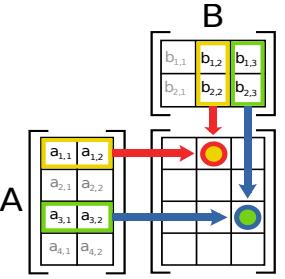
Figure 7.5: Illustration of matrix multiplication. From https: // en. wikipedia. org/ wiki/ Matrix\_ multiplication . Used with kind permission of Wikipedia author Bilou.

Remember that since A ^{→ Rm}↔︎ⁿ and B ^{→ Rn}↔︎^p, ^{ai → Rn} and ^{bj → Rn}, so these inner products all make sense. This is the most “natural” representation when we represent A by rows and B by columns. See Figure 7.5 for an illustration.

Alternatively, we can represent A by columns, and B by rows, which leads to the interpretation of AB as a sum of outer products. Symbolically,

\[\mathbf{C} = \mathbf{AB} = \begin{bmatrix} | & | & & | \\ \mathbf{a}\_1 & \mathbf{a}\_2 & \cdots & \mathbf{a}\_n \\ | & | & & | \end{bmatrix} \begin{bmatrix} - & \mathbf{b}\_1^\top & - \\ - & \mathbf{b}\_2^\top & - \\ & \vdots \\ - & \mathbf{b}\_n^\top & - \end{bmatrix} = \sum\_{i=1}^n \mathbf{a}\_i \mathbf{b}\_i^\top \,. \tag{7.72}\]

Put another way, AB is equal to the sum, over all i, of the outer product of the ith column of A and the ⁱth row of ^B. Since, in this case, ^{ai → Rm} and ^{bi → Rp}, the dimension of the outer product ^aib^T i is m ↓ p, which coincides with the dimension of C.

We can also view matrix-matrix multiplication as a set of matrix-vector products. Specifically, if we represent B by columns, we can view the columns of C as matrix-vector products between A and the columns of B. Symbolically,

\[\mathbf{C} = \mathbf{A}\mathbf{B} = \mathbf{A} \begin{bmatrix} | & | & & | \\ \mathbf{b}\_1 & \mathbf{b}\_2 & \cdots & \mathbf{b}\_p \\ | & | & & | \end{bmatrix} = \begin{bmatrix} | & | & & | \\ \mathbf{A}\mathbf{b}\_1 & \mathbf{A}\mathbf{b}\_2 & \cdots & \mathbf{A}\mathbf{b}\_p \\ | & | & & | \end{bmatrix} . \tag{7.73}\]

Here the ith column of C is given by the matrix-vector product with the vector on the right, cⁱ = Abi. These matrix-vector products can in turn be interpreted using both viewpoints given in the previous subsection.

Finally, we have the analogous viewpoint, where we represent A by rows, and view the rows of C as the matrix-vector product between the rows of A and the matrix B. Symbolically,

\[\mathbf{C} = \mathbf{A}\mathbf{B} = \begin{bmatrix} - & \mathbf{a}\_1^\top & \cdots \\ - & \mathbf{a}\_2^\top & \cdots \\ & \vdots \\ \vdots & & \vdots \\ - & \mathbf{a}\_m^\top & \cdots \end{bmatrix} \mathbf{B} = \begin{bmatrix} - & \mathbf{a}\_1^\top \mathbf{B} & \cdots \\ - & \mathbf{a}\_2^\top \mathbf{B} & \cdots \\ & \vdots \\ - & \mathbf{a}\_m^\top \mathbf{B} & \cdots \end{bmatrix} . \tag{7.74}\]

Here the ith row of C is given by the matrix-vector product with the vector on the left, c^{T i} = a^{T i} B.

It may seem like overkill to dissect matrix multiplication to such a large degree, especially when all these viewpoints follow immediately from the initial definition we gave (in about a line of math) at the beginning of this section. However, virtually all of linear algebra deals with matrix multiplications of some kind, and it is worthwhile to spend some time trying to develop an intuitive understanding of the viewpoints presented here.

Finally, a word on notation. We write A² as shorthand for AA, which is the matrix product. To denote elementwise squaring of the elements of a matrix, we write A↖ ² = [A² ij ]. (If A is diagonal, then A² = A↖ ².)

We can also define the inverse of ^A2 using the matrix square root: we say ^{A = ≃} M if A² = M. To denote elementwise square root of the elements of a matrix, we write [ -Mij ].

7.2.4 Application: manipulating data matrices

As an application of the above results, consider the case where X is the N ↓ D design matrix, whose rows are the data cases. There are various common preprocessing operations that we apply to this matrix, which we summarize below. (Writing these operations in matrix form is useful because it is notationally compact, and it allows us to implement the methods quickly using fast matrix code.)

7.2.4.1 Summing slices of the matrix

Suppose X is an N ↓ D matrix. We can sum across the rows by premultiplying by a 1 ↓ N matrix of ones to create a 1 ↓ D matrix:

\[\mathbf{1}\_N^T \mathbf{X} = \begin{pmatrix} \sum\_n x\_{n1} & \cdots & \sum\_n x\_{nD} \end{pmatrix} \tag{7.75}\]

Hence the mean of the data vectors is given by

\[\overline{\mathbf{x}}^{\mathsf{T}} = \frac{1}{N} \mathbf{1}\_{N}^{\mathsf{T}} \mathbf{X} \tag{7.76}\]

We can sum across the columns by postmultiplying by a D ↓ 1 matrix of ones to create a N ↓ 1 matrix:

\[\mathbf{X1}\_D = \begin{pmatrix} \sum\_d x\_{1d} \\ \vdots \\ \sum\_d x\_{Nd} \end{pmatrix} \tag{7.77}\]

We can sum all entries in a matrix by pre and post multiplying by a vector of 1s:

\[\mathbf{1}\_N^T \mathbf{X} \mathbf{1}\_D = \sum\_{ij} X\_{ij} \tag{7.78}\]

Hence the overall mean is given by

\[\overline{x} = \frac{1}{ND} \mathbf{1}\_N^\mathsf{T} \mathbf{X} \mathbf{1}\_D \tag{7.79}\]

7.2.4.2 Scaling rows and columns of a matrix

We often want to scale rows or columns of a data matrix (e.g., to standardize them). We now show how to write this in matrix notation.

If we pre-multiply X by a diagonal matrix S = diag(s), where s is an N-vector, then we just scale each row of X by the corresponding scale factor in s:

\[\text{diag}(\mathbf{s})\mathbf{X} = \begin{pmatrix} s\_1 & \cdots & 0 \\ & \ddots & \\ 0 & \cdots & s\_N \end{pmatrix} \begin{pmatrix} x\_{1,1} & \cdots & x\_{1,D} \\ & \ddots \\ x\_{N,1} & \cdots & x\_{N,D} \end{pmatrix} = \begin{pmatrix} s\_1 x\_{1,1} & \cdots & s\_1 x\_{1,D} \\ & \ddots \\ & & \ddots \\ s\_N x\_{N,1} & \cdots & s\_N x\_{N,D} \end{pmatrix} \tag{7.80}\]

If we post-multiply X by a diagonal matrix S = diag(s), where s is a D-vector, then we just scale each column of X by the corresponding element in s.

\[\mathbf{Xdiag}(\mathbf{s}) = \begin{pmatrix} x\_{1,1} & \cdots & x\_{1,D} \\ & \ddots & \\ & \ddots & \\ x\_{N,1} & \cdots & x\_{N,D} \end{pmatrix} \begin{pmatrix} s\_1 & \cdots & 0 \\ & \ddots & \\ 0 & \cdots & s\_D \end{pmatrix} = \begin{pmatrix} s\_1 x\_{1,1} & \cdots & s\_D x\_{1,D} \\ & \ddots & \\ & & \ddots \\ s\_1 x\_{N,1} & \cdots & s\_D x\_{N,D} \end{pmatrix} \tag{7.81}\]

Thus we can rewrite the standardization operation from Section 10.2.8 in matrix form as follows:

\[\text{Standardize}(\mathbf{X}) = (\mathbf{X} - \mathbf{1}\_N \boldsymbol{\mu}^T) \text{diag}(\boldsymbol{\sigma})^{-1} \tag{7.82}\]

where µ = x is the empirical mean, and ⇀ is a vector of the empirical standard deviations.

7.2.4.3 Sum of squares and scatter matrix

The sum of squares matrix is D ↓ D matrix defined by

\[\mathbf{S}\_0 \triangleq \mathbf{X}^\mathsf{T} \mathbf{X} = \sum\_{n=1}^N x\_n \mathbf{x}\_n^\mathsf{T} = \sum\_{n=1}^N \begin{pmatrix} x\_{n,1}^2 & \cdots & x\_{n,1} x\_{n,D} \\ & \ddots & \\ x\_{n,D} x\_{n,1} & \cdots & x\_{n,D}^2 \end{pmatrix} \tag{7.83}\]

The scatter matrix is a D ↓ D matrix defined by

\[\mathbf{S}\_{\overline{\mathbf{z}}} \triangleq \sum\_{n=1}^{N} (x\_n - \overline{\mathbf{z}})(x\_n - \overline{\mathbf{z}})^\mathsf{T} = \left(\sum\_{n} x\_n x\_n^\mathsf{T}\right) - N\overline{\mathbf{z}}\overline{\mathbf{z}}^\mathsf{T} \tag{7.84}\]

We see that this is the sum of squares matrix applied to the mean-centered data. More precisely, define X˜ to be a version of X where we subtract the mean x = ^{1 N XT}1^{N o}! every row. Hence we can compute the centered data matrix using

\[\hat{\mathbf{X}} = \mathbf{X} - \mathbf{1}\_N \overline{\mathbf{z}}^\mathsf{T} = \mathbf{X} - \frac{1}{N} \mathbf{1}\_N \mathbf{1}\_N^\mathsf{T} \mathbf{X} = \mathbf{C}\_N \mathbf{X} \tag{7.85}\]

where

\[\mathbf{C}\_{N} \triangleq \mathbf{I}\_{N} - \frac{1}{N} \mathbf{J}\_{N} \tag{7.86}\]

is the centering matrix, and J^N = 1^N 1^{T N} is a matrix of all 1s. The scatter matrix can now be computed as follows:

\[\mathbf{S}\_{\overline{\mathbf{z}}} = \bar{\mathbf{X}}^{\mathsf{T}} \bar{\mathbf{X}} = \mathbf{X}^{\mathsf{T}} \mathbf{C}\_{N}^{\mathsf{T}} \mathbf{C}\_{N} \mathbf{X} = \mathbf{X}^{\mathsf{T}} \mathbf{C}\_{N} \mathbf{X} \tag{7.87}\]

where we exploited the fact that C^N is symmetric and idempotent, i.e., C^{k N} = C^N for k = 1, 2,… (since once we subtract the mean, subtracting it again has no e!ect).

7.2.4.4 Gram matrix

The ^{N ↓ N} matrix XX^T is a matrix of inner products called the Gram matrix:

\[\mathbf{X} \triangleq \mathbf{X} \mathbf{X}^{\top} = \begin{pmatrix} x\_1^{\top} x\_1 & \cdots & x\_1^{\top} x\_N \\ & \ddots & \\ x\_n^{\top} x\_1 & \cdots & x\_N^{\top} x\_N \end{pmatrix} \tag{7.88}\]

Sometimes we want to compute the inner products of the mean-centered data vectors, K˜ = X˜ X˜ ^T. However, if we are working with a feature similarity matrix instead of raw features, we will only have access to K, not X. (We will see examples of this in Section 20.4.4 and Section 20.4.6.) Fortunately, we can compute K˜ from K using the double centering trick:

\[ \tilde{\mathbf{K}} = \tilde{\mathbf{X}} \tilde{\mathbf{X}}^{\mathsf{T}} = \mathbf{C}\_{N} \mathbf{K} \mathbf{C}\_{N} = \mathbf{K} - \frac{1}{N} \mathbf{J} \mathbf{K} - \frac{1}{N} \mathbf{K} \mathbf{J} + \frac{1}{N^{2}} \mathbf{1}^{\mathsf{T}} \mathbf{K} \mathbf{1} \tag{7.89} \]

This subtracts the row means and column means from K, and adds back the global mean that gets subtracted twice, so that both row means and column means of K˜ are equal to zero.

To see why Equation (7.89) is true, consider the scalar form:

\[\bar{K}\_{ij} = \bar{x}\_i^\top \bar{x}\_j = (x\_i - \frac{1}{N} \sum\_{k=1}^N x\_k)(x\_j - \frac{1}{N} \sum\_{l=1}^N x\_l) \tag{7.90}\]

\[\mathbf{x} = \mathbf{x}\_i^\mathsf{T} \mathbf{x}\_j - \frac{1}{N} \sum\_{k=1}^N \mathbf{x}\_i^\mathsf{T} \mathbf{x}\_k - \frac{1}{N} \sum\_{k=1}^N \mathbf{x}\_j^\mathsf{T} \mathbf{x}\_k + \frac{1}{N^2} \sum\_{k=1}^N \sum\_{l=1}^N \mathbf{x}\_k^\mathsf{T} \mathbf{x}\_l \tag{7.91}\]

7.2.4.5 Distance matrix

Let X be N^x ↓ D datamatrix, and Y be another N^y ↓ D datamatrix. We can compute the squared pairwise distances between these using

\[\mathbf{D}\_{ij} = (\mathbf{x}\_i - \mathbf{y}\_j)^\mathsf{T}(\mathbf{x}\_i - \mathbf{y}\_j) = ||\mathbf{x}\_i||^2 - 2\mathbf{x}\_i^\mathsf{T}\mathbf{y}\_j + ||\mathbf{y}\_j||^2\tag{7.92}\]

Let us now write this in matrix form. Let ^xˆ = [||x1||²; ··· ; ||x^Nx ||²] = diag(XXT) be a vector where each element is the squared norm of the examples in X, and define yˆ similarly. Then we have

\[\mathbf{D} = \hat{\mathbf{x}} \mathbf{1}\_{N\_y}^{\mathsf{T}} - 2\mathbf{X}\mathbf{Y}^{\mathsf{T}} + \mathbf{1}\_{N\_x}\hat{\mathbf{y}}^{\mathsf{T}} \tag{7.93}\]

In the case that X = Y, we have

\[\mathbf{D} = \hat{\mathbf{x}}\mathbf{1}\_N^\mathsf{T} - 2\mathbf{X}\mathbf{X}^\mathsf{T} + \mathbf{1}\_N \hat{\mathbf{x}}^\mathsf{T} \tag{7.94}\]

This vectorized computation is often much faster than using for loops.

7.2.5 Kronecker products *

If A is an m↓n matrix and B is a p↓q matrix, then the Kronecker product A△ B is the mp↓nq block matrix

\[\mathbf{A} \otimes \mathbf{B} = \begin{bmatrix} a\_{11}\mathbf{B} & \cdots & a\_{1n}\mathbf{B} \\ \vdots & \ddots & \vdots \\ a\_{m1}\mathbf{B} & \cdots & a\_{mn}\mathbf{B} \end{bmatrix} \tag{7.95}\]

For example,

\[ \begin{bmatrix} a\_{11} & a\_{12} \\ a\_{21} & a\_{22} \\ a\_{31} & a\_{32} \end{bmatrix} \otimes \begin{bmatrix} b\_{11} & b\_{12} & b\_{13} \\ b\_{21} & b\_{22} & b\_{23} \end{bmatrix} = \begin{bmatrix} a\_{11}b\_{11} & a\_{11}b\_{12} & a\_{11}b\_{13} & a\_{12}b\_{11} & a\_{12}b\_{12} & a\_{12}b\_{13} \\ a\_{11}b\_{21} & a\_{11}b\_{22} & a\_{11}b\_{23} & a\_{12}b\_{21} & a\_{12}b\_{22} & a\_{12}b\_{23} \\ a\_{21}b\_{11} & a\_{21}b\_{12} & a\_{21}b\_{13} & a\_{22}b\_{11} & a\_{22}b\_{12} & a\_{22}b\_{13} \\ a\_{21}b\_{21} & a\_{21}b\_{22} & a\_{21}b\_{23} & a\_{22}b\_{21} & a\_{22}b\_{22} & a\_{22}b\_{23} \\ a\_{31}b\_{11} & a\_{31}b\_{12} & a\_{31}b\_{13} & a\_{32}b\_{11} & a\_{32}b\_{12} & a\_{32}b\_{13} \\ a\_{31}b\_{21} & a\_{31}b\_{22} & a\_{31}b\_{23} & a\_{32}b\_{21} & a\_{32}b\_{22} & a\_{32}b\_{23} \end{bmatrix} \tag{7.96} \]

Here are some useful identities:

\[(\mathbf{A}\otimes\mathbf{B})^{-1}=\mathbf{A}^{-1}\otimes\mathbf{B}^{-1}\tag{7.97}\]

\[(\mathbf{A} \otimes \mathbf{B}) \text{vec}(\mathbf{C}) = \text{vec}(\mathbf{BCA}^{\sf T}) \tag{7.98}\]

where vec(M) stacks the columns of M. (If we stack along the rows, we get (A △ B)vec(C) = vec(ACB^T).) See [Loa00] for a list of other useful properties.

7.2.6 Einstein summation *

Einstein summation, or einsum for short, is a notational shortcut for working with tensors. The convention was introduced by Einstein [Ein16, sec 5], who later joked to a friend, “I have made a great discovery in mathematics; I have suppressed the summation sign every time that the summation must be made over an index which occurs twice…” [Pai05, p.216]. For example, instead of writing matrix multiplication as Cij = $ $ ^k AikBkj , we can just write it as Cij = AikBkj , where we drop the k.

As a more complex example, suppose we have a 3d tensor Sntk where n indexes examples in the batch, t indexes locations in the sequence, and k indexes words in a one-hot representation. Let Wkd be an embedding matrix that maps sparse one-hot vectors R^k to dense vectors in R^d. We can convert the batch of sequences of one-hots to a batch of sequences of embeddings as follows:

\[E\_{ntd} = \sum\_{k} S\_{ntk} W\_{kd} \tag{7.99}\]

We can compute the sum of the embedding vectors for each sequence (to get a global representation of each bag of words) as follows:

\[E\_{nd} = \sum\_{k} \sum\_{t} S\_{ntk} W\_{kd} \tag{7.100}\]

Finally we can pass each sequence’s vector representation through another linear transform Vdc to map to the logits over a classifier with c labels:

\[L\_{nc} = \sum\_{d} E\_{nd} V\_{dc} = \sum\_{d} \sum\_{k} \sum\_{t} S\_{ntk} W\_{kd} V\_{dc} \tag{7.101}\]

In einsum notation, we write Lnc = SntkWkdVdc. We sum over k and d because those indices occur twice on the RHS. We sum over t because that index does not occur on the LHS.

Einsum is implemented in NumPy, Tensorflow, PyTorch, etc. What makes it particularly useful is that it can perform the relevant tensor multiplications in complex expressions in an optimal order, so as to minimize time and intermediate memory allocation.2 The library is best illustrated by the examples in einsum\_demo.ipynb.

Note that the speed of einsum depends on the order in which the operations are performed, which depends on the shapes of the relevant arguments. The optimal ordering minimizes the treewidth of the resulting computation graph, as explained in [GASG18]. In general, the time to compute the optimal ordering is exponential in the number of arguments, so it is common to use a greedy approximation. However, if we expect to repeat the same calculation many times, using tensors of the same shape but potentially di!erent content, we can compute the optimal ordering once and reuse it multiple times.

7.3 Matrix inversion

In this section, we discuss how to invert di!erent kinds of matrices.

7.3.1 The inverse of a square matrix

The inverse of a square matrix ^{A → Rn}↔︎ⁿ is denoted ^A→¹, and is the unique matrix such that

\[\mathbf{A}^{-1}\mathbf{A} = \mathbf{I} = \mathbf{A}\mathbf{A}^{-1}.\tag{7.102}\]

Note that ^A→¹ exists if and only if det(A) ↗= 0. If det(A)=0, it is called a singular matrix.

The following are properties of the inverse; all assume that ^A, ^{B → Rn}↔︎ⁿ are non-singular:

\[(\mathbf{A}^{-1})^{-1} = \mathbf{A} \tag{7.103}\]

\[(\mathbf{A}\mathbf{B})^{-1} = \mathbf{B}^{-1}\mathbf{A}^{-1} \tag{7.104}\]

\[(\mathbf{A}^{-1})^{\mathsf{T}} = (\mathbf{A}^{\mathsf{T}})^{-1} \stackrel{\scriptstyle \Delta}{=} \mathbf{A}^{-T} \tag{7.105}\]

For the case of a ^{2 ↓ 2} matrix, the expression for ^A→¹ is simple enough to give explicitly. We have

\[\mathbf{A} = \begin{pmatrix} a & b \\ c & d \end{pmatrix}, \quad \mathbf{A}^{-1} = \frac{1}{|\mathbf{A}|} \begin{pmatrix} d & -b \\ -c & a \end{pmatrix} \tag{7.106}\]

For a block diagonal matrix, the inverse is obtained by simply inverting each block separately, e.g.,

\[ \begin{pmatrix} \mathbf{A} & \mathbf{0} \\ \mathbf{0} & \mathbf{B} \end{pmatrix}^{-1} = \begin{pmatrix} \mathbf{A}^{-1} & \mathbf{0} \\ \mathbf{0} & \mathbf{B}^{-1} \end{pmatrix} \tag{7.107} \]

2. These optimizations are implemented in the opt-einsum library [GASG18]. Its core functionality is included in NumPy and JAX einsum functions, provided you set optimize=True parameter.

7.3.2 Schur complements *

In this section, we review some useful results concerning block structured matrices.

Theorem 7.3.1 (Inverse of a partitioned matrix). Consider a general partitioned matrix

\[\mathbf{M} = \begin{pmatrix} \mathbf{E} & \mathbf{F} \\ \mathbf{G} & \mathbf{H} \end{pmatrix} \tag{7.108}\]

where we assume E and H are invertible. We have

\[\mathbf{M}^{-1} = \begin{pmatrix} (\mathbf{M}/\mathbf{H})^{-1} & -(\mathbf{M}/\mathbf{H})^{-1}\mathbf{F}\mathbf{H}^{-1} \\ -\mathbf{H}^{-1}\mathbf{G}(\mathbf{M}/\mathbf{H})^{-1} & \mathbf{H}^{-1} + \mathbf{H}^{-1}\mathbf{G}(\mathbf{M}/\mathbf{H})^{-1}\mathbf{F}\mathbf{H}^{-1} \\ \ddots & \ddots \end{pmatrix} \tag{7.109}\]

\[\begin{aligned} \mathbf{E} = \begin{pmatrix} \mathbf{E}^{-1} + \mathbf{E}^{-1} \mathbf{F} (\mathbf{M}/\mathbf{E})^{-1} \mathbf{G} \mathbf{E}^{-1} & -\mathbf{E}^{-1} \mathbf{F} (\mathbf{M}/\mathbf{E})^{-1} \\ -(\mathbf{M}/\mathbf{E})^{-1} \mathbf{G} \mathbf{E}^{-1} & (\mathbf{M}/\mathbf{E})^{-1} \end{pmatrix} \end{aligned} \tag{7.110}\]

where

\[\mathbf{M}/\mathbf{H} \stackrel{\Delta}{=} \mathbf{E} - \mathbf{F}\mathbf{H}^{-1}\mathbf{G} \tag{7.111}\]

\[\mathbf{M}/\mathbf{E} \stackrel{\triangle}{=} \mathbf{H} - \mathbf{G}\mathbf{E}^{-1}\mathbf{F} \tag{7.112}\]

We say that M/H is the Schur complement of M wrt H, and M/E is the Schur complement of M wrt E.

Equation (7.109) and Equation (7.110) are called the partitioned inverse formulae.

Proof. If we could block diagonalize M, it would be easier to invert. To zero out the top right block of M we can pre-multiply as follows

\[ \begin{pmatrix} \mathbf{I} & -\mathbf{F}\mathbf{H}^{-1} \\ \mathbf{0} & \mathbf{I} \end{pmatrix} \begin{pmatrix} \mathbf{E} & \mathbf{F} \\ \mathbf{G} & \mathbf{H} \end{pmatrix} = \begin{pmatrix} \mathbf{E} - \mathbf{F}\mathbf{H}^{-1}\mathbf{G} & \mathbf{0} \\ \mathbf{G} & \mathbf{H} \end{pmatrix} \tag{7.113} \]

Similarly, to zero out the bottom left we can post-multiply as follows

\[ \begin{pmatrix} \mathbf{E} - \mathbf{F} \mathbf{H}^{-1} \mathbf{G} & \mathbf{0} \\ \mathbf{G} & \mathbf{H} \end{pmatrix} \begin{pmatrix} \mathbf{I} & \mathbf{0} \\ -\mathbf{H}^{-1} \mathbf{G} & \mathbf{I} \end{pmatrix} = \begin{pmatrix} \mathbf{E} - \mathbf{F} \mathbf{H}^{-1} \mathbf{G} & \mathbf{0} \\ \mathbf{0} & \mathbf{H} \end{pmatrix} \tag{7.114} \]

Putting it all together we get

\[\underbrace{\begin{pmatrix} \mathbf{I} & -\mathbf{F}\mathbf{H}^{-1} \\ \mathbf{0} & \mathbf{I} \end{pmatrix}}\_{\mathbf{X}} \underbrace{\begin{pmatrix} \mathbf{E} & \mathbf{F} \\ \mathbf{G} & \mathbf{H} \end{pmatrix}}\_{\mathbf{M}} \underbrace{\begin{pmatrix} \mathbf{I} & \mathbf{0} \\ -\mathbf{H}^{-1}\mathbf{G} & \mathbf{I} \end{pmatrix}}\_{\mathbf{Z}} = \underbrace{\begin{pmatrix} \mathbf{E} - \mathbf{F}\mathbf{H}^{-1}\mathbf{G} & \mathbf{0} \\ \mathbf{0} & \mathbf{H} \end{pmatrix}}\_{\mathbf{W}} \tag{7.115}\]

Taking the inverse of both sides yields

\[\mathbf{Z}^{-1}\mathbf{M}^{-1}\mathbf{X}^{-1} = \mathbf{W}^{-1}\tag{7.116}\]

\[\mathbf{M}^{-1} = \mathbf{Z}\mathbf{W}^{-1}\mathbf{X}\tag{7.117}\]

Substituting in the definitions we get

\[ \begin{pmatrix} \mathbf{E} & \mathbf{F} \\ \mathbf{G} & \mathbf{H} \end{pmatrix}^{-1} = \begin{pmatrix} \mathbf{I} & \mathbf{0} \\ -\mathbf{H}^{-1}\mathbf{G} & \mathbf{I} \end{pmatrix} \begin{pmatrix} (\mathbf{M}/\mathbf{H})^{-1} & \mathbf{0} \\ \mathbf{0} & \mathbf{H}^{-1} \end{pmatrix} \begin{pmatrix} \mathbf{I} & -\mathbf{F}\mathbf{H}^{-1} \\ \mathbf{0} & \mathbf{I} \end{pmatrix} \tag{7.118} \]

\[\begin{aligned} \mathbf{H} &= \begin{pmatrix} (\mathbf{M}/\mathbf{H})^{-1} & \mathbf{0} \\ -\mathbf{H}^{-1}\mathbf{G}(\mathbf{M}/\mathbf{H})^{-1} & \mathbf{H}^{-1} \end{pmatrix} \begin{pmatrix} \mathbf{I} & -\mathbf{F}\mathbf{H}^{-1} \\ \mathbf{0} & \mathbf{I} \end{pmatrix} \end{aligned} \tag{7.119}\]

\[=\begin{pmatrix} (\mathbf{M}/\mathbf{H})^{-1} & -(\mathbf{M}/\mathbf{H})^{-1}\mathbf{F}\mathbf{H}^{-1} \\ -\mathbf{H}^{-1}\mathbf{G}(\mathbf{M}/\mathbf{H})^{-1} & \mathbf{H}^{-1} + \mathbf{H}^{-1}\mathbf{G}(\mathbf{M}/\mathbf{H})^{-1}\mathbf{F}\mathbf{H}^{-1} \end{pmatrix} \tag{7.120}\]

Alternatively, we could have decomposed the matrix M in terms of E and M/E = (H ^↑ GE→¹F), yielding

\[ \begin{pmatrix} \mathbf{E} & \mathbf{F} \\ \mathbf{G} & \mathbf{H} \end{pmatrix}^{-1} = \begin{pmatrix} \mathbf{E}^{-1} + \mathbf{E}^{-1} \mathbf{F} (\mathbf{M}/\mathbf{E})^{-1} \mathbf{G} \mathbf{E}^{-1} & -\mathbf{E}^{-1} \mathbf{F} (\mathbf{M}/\mathbf{E})^{-1} \\ -(\mathbf{M}/\mathbf{E})^{-1} \mathbf{G} \mathbf{E}^{-1} & (\mathbf{M}/\mathbf{E})^{-1} \end{pmatrix} \tag{7.121} \]

7.3.3 The matrix inversion lemma *

Equating the top left block of the first matrix in Equation (7.119) with the top left block of the matrix in Equation (7.121)

\[\left(\mathbf{M}/\mathbf{H}\right)^{-1} = \left(\mathbf{E} - \mathbf{F}\mathbf{H}^{-1}\mathbf{G}\right)^{-1} = \mathbf{E}^{-1} + \mathbf{E}^{-1}\mathbf{F}(\mathbf{H} - \mathbf{G}\mathbf{E}^{-1}\mathbf{F})^{-1}\mathbf{G}\mathbf{E}^{-1} \tag{7.122}\]

This is known as the matrix inversion lemma or the Sherman-Morrison-Woodbury formula.

A typical application in machine learning is the following. Let X be an N ↓ D data matrix, and ! be ^{N ↓ N} diagonal matrix. Then we have (using the substitutions E = !, F = G^T = X, and ^H→^{1 = ↑}I) the following result:

\[(\boldsymbol{\Sigma} + \mathbf{X}\mathbf{X}^{\mathsf{T}})^{-1} = \boldsymbol{\Sigma}^{-1} - \boldsymbol{\Sigma}^{-1}\mathbf{X}(\mathbf{I} + \mathbf{X}^{\mathsf{T}}\boldsymbol{\Sigma}^{-1}\mathbf{X})^{-1}\mathbf{X}^{\mathsf{T}}\boldsymbol{\Sigma}^{-1} \tag{7.123}\]

The LHS takes O(N³) time to compute, the RHS takes time O(D³) to compute.

Another application concerns computing a rank one update of an inverse matrix. Let E = A, ^{F = u}, ^{G = vT}, and ^{H = ↑}1. Then we have

\[(\mathbf{A} + u\mathbf{v}^{\mathsf{T}})^{-1} = \mathbf{A}^{-1} + \mathbf{A}^{-1}u(-1 - \mathbf{v}^{\mathsf{T}}\mathbf{A}^{-1}u)^{-1}\mathbf{v}^{\mathsf{T}}\mathbf{A}^{-1} \tag{7.124}\]

\[=\mathbf{A}^{-1} - \frac{\mathbf{A}^{-1}uv^{\top}\mathbf{A}^{-1}}{1 + v^{\top}\mathbf{A}^{-1}u} \tag{7.125}\]

This is known as the Sherman-Morrison formula.

7.3.4 Matrix determinant lemma *

We now use the above results to derive an e”cient way to compute the determinant of a blockstructured matrix.

From Equation (7.115), we have

\[|\mathbf{X}||\mathbf{M}||\mathbf{Z}| = |\mathbf{W}| = |\mathbf{E} - \mathbf{F}\mathbf{H}^{-1}\mathbf{G}||\mathbf{H}|\tag{7.126}\]

\[\begin{aligned} \left| \begin{pmatrix} \mathbf{E} & \mathbf{F} \\ \mathbf{G} & \mathbf{H} \end{pmatrix} \right| &= \left| \mathbf{E} - \mathbf{F} \mathbf{H}^{-1} \mathbf{G} \right|| \left| \mathbf{H} \right| \end{aligned} \tag{7.127}\]

\[|\mathbf{M}| = |\mathbf{M}/\mathbf{H}||\mathbf{H}|\tag{7.128}\]

\[|\mathbf{M}/\mathbf{H}| = \frac{|\mathbf{M}|}{|\mathbf{H}|}\tag{7.129}\]

So we can see that M/H acts somewhat like a division operator (hence the notation).

Furthermore, we have

\[|\mathbf{M}| = |\mathbf{M}/\mathbf{H}||\mathbf{H}| = |\mathbf{M}/\mathbf{E}||\mathbf{E}|\tag{7.130}\]

\[|\mathbf{M}/\mathbf{H}| = \frac{|\mathbf{M}/\mathbf{E}||\mathbf{E}|}{|\mathbf{H}|} \tag{7.131}\]

\[|\mathbf{E} - \mathbf{F}\mathbf{H}^{-1}\mathbf{G}| = |\mathbf{H} - \mathbf{G}\mathbf{E}^{-1}\mathbf{F}||\mathbf{H}^{-1}||\mathbf{E}|\tag{7.132}\]

Hence (setting ^{E = A}, ^{F = ↑}u, ^{G = vT}, ^H = 1) we have

\[|\mathbf{A} + \mathbf{u}\mathbf{v}^{\mathrm{T}}| = (1 + \mathbf{v}^{\mathrm{T}}\mathbf{A}^{-1}\mathbf{u})|\mathbf{A}|\tag{7.133}\]

This is known as the matrix determinant lemma.

7.3.5 Application: deriving the conditionals of an MVN *

Consider a joint Gaussian of the form p(x1, x2) = N (x|µ, !), where

\[ \mu = \begin{pmatrix} \mu\_1 \\ \mu\_2 \end{pmatrix}, \quad \Sigma = \begin{pmatrix} \Sigma\_{11} & \Sigma\_{12} \\ \Sigma\_{21} & \Sigma\_{22} \end{pmatrix} \tag{7.134} \]

In Section 3.2.3, we claimed that

\[p(\mathbf{x}\_1|\mathbf{x}\_2) = \mathcal{N}(\mathbf{x}\_1|\boldsymbol{\mu}\_1 + \boldsymbol{\Sigma}\_{12}\boldsymbol{\Sigma}\_{22}^{-1}(\mathbf{x}\_2 - \boldsymbol{\mu}\_2), \ \boldsymbol{\Sigma}\_{11} - \boldsymbol{\Sigma}\_{12}\boldsymbol{\Sigma}\_{22}^{-1}\boldsymbol{\Sigma}\_{21})\tag{7.135}\]

In this section, we derive this result using Schur complements.

Let us factor the joint p(x1, x2) as p(x2)p(x1|x2) as follows:

\[p(\mathbf{z}\_1, \mathbf{z}\_2) \propto \exp\left\{ -\frac{1}{2} \begin{pmatrix} \mathbf{z}\_1 - \mu\_1\\ \mathbf{z}\_2 - \mu\_2 \end{pmatrix}^{\mathsf{T}} \begin{pmatrix} \Sigma\_{11} & \Sigma\_{12} \\ \Sigma\_{21} & \Sigma\_{22} \end{pmatrix}^{-1} \begin{pmatrix} \mathbf{z}\_1 - \mu\_1\\ \mathbf{z}\_2 - \mu\_2 \end{pmatrix} \right\} \tag{7.136}\]

Using Equation (7.118) the above exponent becomes

\[p(\boldsymbol{x}\_{1}, \boldsymbol{x}\_{2}) \propto \exp\left\{-\frac{1}{2} \begin{pmatrix} \boldsymbol{x}\_{1} - \boldsymbol{\mu}\_{1} \\ \boldsymbol{x}\_{2} - \boldsymbol{\mu}\_{2} \end{pmatrix}^{\mathsf{T}} \begin{pmatrix} \mathbf{I} & \mathbf{0} \\ -\boldsymbol{\Sigma}\_{22}^{-1} \boldsymbol{\Sigma}\_{21} & \mathbf{I} \end{pmatrix} \begin{pmatrix} (\boldsymbol{\Sigma}/\boldsymbol{\Sigma}\_{22})^{-1} & \mathbf{0} \\ \mathbf{0} & \boldsymbol{\Sigma}\_{22}^{-1} \end{pmatrix} \tag{7.137}\]

\[\times \begin{pmatrix} \mathbf{I} & -\Sigma\_{12}\Sigma\_{22}^{-1} \\ \mathbf{0} & \mathbf{I} \end{pmatrix} \begin{pmatrix} x\_1 - \mu\_1 \\ x\_2 - \mu\_2 \end{pmatrix} \end{pmatrix} \tag{7.138}\]

\[=\exp\left\{-\frac{1}{2}(\boldsymbol{x}\_{1}-\boldsymbol{\mu}\_{1}-\boldsymbol{\Sigma}\_{12}\boldsymbol{\Sigma}\_{22}^{-1}(\boldsymbol{x}\_{2}-\boldsymbol{\mu}\_{2}))^{\mathsf{T}}(\boldsymbol{\Sigma}/\boldsymbol{\Sigma}\_{22})^{-1}\right\}\tag{7.139}\]

\[\left\{ (\boldsymbol{x}\_{1} - \boldsymbol{\mu}\_{1} - \boldsymbol{\Sigma}\_{12} \boldsymbol{\Sigma}\_{22}^{-1} (\boldsymbol{x}\_{2} - \boldsymbol{\mu}\_{2})) \right\} \times \exp\left\{ -\frac{1}{2} (\boldsymbol{x}\_{2} - \boldsymbol{\mu}\_{2})^{\mathsf{T}} \boldsymbol{\Sigma}\_{22}^{-1} (\boldsymbol{x}\_{2} - \boldsymbol{\mu}\_{2}) \right\} \tag{7.140}\]

This is of the form

\[\exp(\text{quadratic form in } \mathbf{z}\_1, \mathbf{z}\_2) \times \exp(\text{quadratic form in } \mathbf{z}\_2) \tag{7.141}\]

Hence we have successfully factorized the joint as

\[p(\mathbf{x}\_1, \mathbf{x}\_2) = p(\mathbf{x}\_1 | \mathbf{x}\_2) p(\mathbf{x}\_2) \tag{7.142}\]

\[=\mathcal{N}(x\_1|\mu\_{1|2},\Sigma\_{1|2})\mathcal{N}(x\_2|\mu\_2,\Sigma\_{22})\tag{7.143}\]

where the parameters of the conditional distribution can be read o! from the above equations using

\[ \mu\_{1|2} = \mu\_1 + \Sigma\_{12} \Sigma\_{22}^{-1} (x\_2 - \mu\_2) \tag{7.144} \]

\[ \Delta\Sigma\_{1|2} = \Sigma/\Sigma\_{22} = \Sigma\_{11} - \Sigma\_{12}\Sigma\_{22}^{-1}\Sigma\_{21} \tag{7.145} \]

We can also use the fact that |M| = |M/H||H| to check the normalization constants are correct:

\[(2\pi)^{(d\_1+d\_2)/2} |\Sigma|^{\frac{1}{2}} = (2\pi)^{(d\_1+d\_2)/2} (|\Sigma/\Sigma\_{22}| \ |\Sigma\_{22}|)^{\frac{1}{2}} \tag{7.146}\]

\[= (2\pi)^{d\_1/2} |\Sigma/\Sigma\_{22}|^{\frac{1}{2}} \left( 2\pi \right)^{d\_2/2} |\Sigma\_{22}|^{\frac{1}{2}} \tag{7.147}\]

where d¹ = dim(x1) and d² = dim(x2).

7.4 Eigenvalue decomposition (EVD)

In this section, we review some standard material on the eigenvalue decomposition or EVD of square (real-valued) matrices.

7.4.1 Basics

Given a square matrix A ^{→ Rn}↔︎ⁿ, we say that ^{φ → R} is an eigenvalue of A and ^{u → Rn} is the corresponding eigenvector if

\[\mathbf{A}u = \lambda u, \quad u \neq 0 \; . \tag{7.148}\]

Intuitively, this definition means that multiplying A by the vector u results in a new vector that points in the same direction as u, but is scaled by a factor φ. For example, if A is a rotation matrix, then u is the axis of rotation and φ = 1.

Note that for any eigenvector ^{u → R}n, and scalar ^{c → R},

\[\mathbf{A}(c\mathbf{u}) = c\mathbf{A}\mathbf{u} = c\lambda\mathbf{u} = \lambda(c\mathbf{u})\tag{7.149}\]

Hence cu is also an eigenvector. For this reason when we talk about “the” eigenvector associated with φ, we usually assume that the eigenvector is normalized to have length 1 (this still creates some ambiguity, since u and ↑u will both be eigenvectors, but we will have to live with this).

We can rewrite the equation above to state that (φ, x) is an eigenvalue-eigenvector pair of A if

\[(\lambda \mathbf{I} - \mathbf{A})\mathbf{u} = \mathbf{0}, \quad \mathbf{u} \neq \mathbf{0} \; \text{ .} \tag{7.150}\]

Now (φI ↑ A)u = 0 has a non-zero solution to u if and only if (φI ↑ A) has a non-empty nullspace, which is only the case if (φI ↑ A) is singular, i.e.,

\[\det(\lambda \mathbf{I} - \mathbf{A}) = 0 \; . \tag{7.151}\]

This is called the characteristic equation of A. (See Exercise 7.2.) The n solutions of this equation are the n (possibly complex-valued) eigenvalues φi, and uⁱ are the corresponding eigenvectors. It is standard to sort the eigenvectors in order of their eigenvalues, with the largest magnitude ones first.

The following are properties of eigenvalues and eigenvectors.

• The trace of a matrix is equal to the sum of its eigenvalues,

\[\text{tr}(\mathbf{A}) = \sum\_{i=1}^{n} \lambda\_i \quad . \tag{7.152}\]

• The determinant of A is equal to the product of its eigenvalues,

\[\det(\mathbf{A}) = \prod\_{i=1}^{n} \lambda\_i \quad . \tag{7.153}\]

• The rank of A is equal to the number of non-zero eigenvalues of A.
• If A is non-singular then 1/φⁱ is an eigenvalue of A→¹ with associated eigenvector ui, i.e., A→¹uⁱ = (1/φi)ui.
• The eigenvalues of a diagonal or triangular matrix are just the diagonal entries.

7.4.2 Diagonalization

We can write all the eigenvector equations simultaneously as

\[\mathbf{AU} = \mathbf{U}\boldsymbol{\Lambda}\tag{7.154}\]

where the columns of ^{U → R}n↔︎ⁿ are the eigenvectors of ^A and ” is a diagonal matrix whose entries are the eigenvalues of A, i.e.,

\[\mathbf{U} \in \mathbb{R}^{n \times n} = \left[ \begin{array}{c} | & | & | \\ \mathbf{u}\_1 & \mathbf{u}\_2 & \cdots & \mathbf{u}\_n \\ | & | & | \end{array} \right], \ \mathbf{A} = \text{diag}(\lambda\_1, \dots, \lambda\_n) \ . \tag{7.155}\]

If the eigenvectors of A are linearly independent, then the matrix U will be invertible, so

\[\mathbf{A} = \mathbf{U}\mathbf{A}\mathbf{U}^{-1}.\tag{7.156}\]

A matrix that can be written in this form is called diagonalizable.

7.4.3 Eigenvalues and eigenvectors of symmetric matrices

When A is real and symmetric, it can be shown that all the eigenvalues are real, and the eigenvectors are orthonormal, i.e., u^{T i uj} = 0 if ⁱ ↗= ^j, and ^{uT i} uⁱ = 1, where uⁱ are the eigenvectors. In matrix form, this becomes U^TU = UU^T = I; hence we see that U is an orthogonal matrix.

We can therefore represent A as

\[\mathbf{A} = \mathbf{U}\mathbf{A}\mathbf{U}^{\top} = \begin{pmatrix} | & | & & | \\ \mathbf{u}\_1 & \mathbf{u}\_2 & \cdots & \mathbf{u}\_n \\ | & | & & | \end{pmatrix} \begin{pmatrix} \lambda\_1 & & & \\ & \lambda\_2 & & \\ & & \ddots & \\ & & & \lambda\_n \end{pmatrix} \begin{pmatrix} - & \mathbf{u}\_1^\top & - \\ - & \mathbf{u}\_2^\top & - \\ & \vdots & \\ - & \mathbf{u}\_n^\top & - \end{pmatrix} \tag{7.157}\]

\[\mathbf{u} = \lambda\_1 \begin{pmatrix} | \\ u\_1 \\ | \end{pmatrix} \begin{pmatrix} - & u\_1^\mathsf{T} & - \end{pmatrix} + \dots + \lambda\_n \begin{pmatrix} | \\ u\_n \\ | \end{pmatrix} \begin{pmatrix} - & u\_n^\mathsf{T} & - \end{pmatrix} = \sum\_{i=1}^n \lambda\_i u\_i u\_i^\mathsf{T} \tag{7.158}\]

Thus multiplying by any symmetric matrix A can be interpreted as multiplying by a rotation matrix U^T, a scaling matrix “, followed by an inverse rotation U.

Once we have diagonalized a matrix, it is easy to invert. Since A = U”UT, where U^T = U→1, we have

\[\mathbf{A}^{-1} = \mathbf{U}\boldsymbol{\Lambda}^{-1}\mathbf{U}^{\mathrm{T}} = \sum\_{i=1}^{d} \frac{1}{\lambda\_i} \mathbf{u}\_i \mathbf{u}\_i^{\mathrm{T}} \tag{7.159}\]

This corresponds to rotating, unscaling, and then rotating back.

7.4.3.1 Checking for positive definiteness

We can also use the diagonalization property to show that a symmetric matrix is positive definite i! all its eigenvalues are positive. To see this, note that

\[\mathbf{x}^{\mathsf{T}}\mathbf{A}\mathbf{x} = \mathbf{x}^{\mathsf{T}}\mathbf{U}\boldsymbol{\Lambda}\mathbf{U}^{\mathsf{T}}\mathbf{x} = \mathbf{y}^{\mathsf{T}}\boldsymbol{\Lambda}\mathbf{y} = \sum\_{i=1}^{n} \lambda\_{i} y\_{i}^{2} \tag{7.160}\]

where y = U^Tx. Because y^{2 i} is always nonnegative, the sign of this expression depends entirely on the φi’s. If all φⁱ > 0, then the matrix is positive definite; if all φⁱ ∋ 0, it is positive semidefinite. Likewise, if all φⁱ < 0 or φⁱ ↘ 0, then A is negative definite or negative semidefinite respectively. Finally, if A has both positive and negative eigenvalues, it is indefinite.

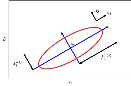
Figure 7.6: Visualization of a level set of the quadratic form (x ↑ µ) ^TA(^{x ↑ µ}) in 2d. The major and minor axes of the ellipse are defined by the first two eigenvectors of A, namely u¹ and u2. Adapted from Figure 2.7 of [Bis06]. Generated by gaussEvec.ipynb.

7.4.4 Geometry of quadratic forms

A quadratic form is a function that can be written as

\[f(x) = x^{\top} \mathbf{A} x \tag{7.161}\]

where ^{x → Rn} and A is a positive definite, symmetric ⁿ-by-ⁿ matrix. Let A = U”U^T be a diagonalization of A (see Section 7.4.3). Hence we can write

\[f(\mathbf{x}) = \mathbf{x}^{\mathsf{T}} \mathbf{A} \mathbf{x} = \mathbf{x}^{\mathsf{T}} \mathbf{U} \mathbf{A} \mathbf{U}^{\mathsf{T}} \mathbf{x} = \mathbf{y}^{\mathsf{T}} \boldsymbol{\Lambda} \mathbf{y} = \sum\_{i=1}^{n} \lambda\_{i} y\_{i}^{2} \tag{7.162}\]

where yⁱ = x^Tuⁱ and φⁱ > 0 (since A is positive definite). The level sets of f(x) define hyper-ellipsoids. For example, in 2d, we have

\[ \lambda\_1 y\_1^2 + \lambda\_2 y\_2^2 = r \tag{7.163} \]

which is the equation of a 2d ellipse. This is illustrated in Figure 7.6. The eigenvectors determine the orientation of the ellipse, and the eigenvalues determine how elongated it is. In particular, the major and minor semi-axes of the ellipse satisfy a→² = φ¹ and b→² = φ2. In the case of a Gaussian distribution, we have A = !^→1, so small values of φⁱ correspond to directions where the posterior has low precision and hence high variance.

7.4.5 Standardizing and whitening data

Suppose we have a dataset ^{X → RN}↔︎D. It is common to preprocess the data so that each column has zero mean and unit variance. This is called standardizing the data, as we discuss in Section 10.2.8. Although standardizing forces the variance to be 1, it does not remove correlation between the columns. To do that, we must whiten the data. To define this, let the empirical covariance matrix

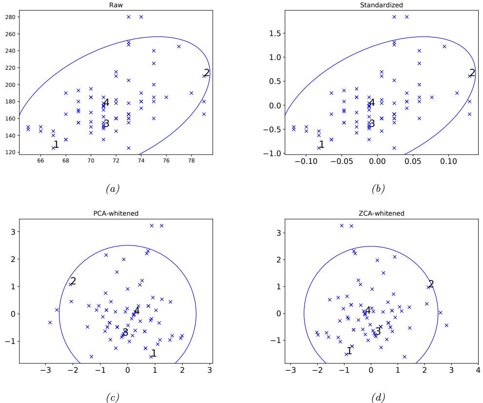
Figure 7.7: (a) Height/weight data. (b) Standardized. (c) PCA Whitening. (d) ZCA whitening. Numbers refer to the first 4 datapoints, but there are 73 datapoints in total. Generated by height\_weight\_whiten\_plot.ipynb.

be ! = ^{1 N X}TX, and let ! ⁼ EDE^T be its diagonalization. Equivalently, let [U, ^S, ^V] be the SVD of ⇐ 1 ^{N X} (so ^{E = V} and ^{D = S2}, as we discuss in Section 20.1.3.3.) Now define

\[\mathbf{W}\_{\rm pca} = \mathbf{D}^{-\frac{1}{2}} \mathbf{E}^{T} \tag{7.164}\]

This is called the PCA whitening matrix. (We discuss PCA in Section 20.1.) Let y = Wpcax be a transformed vector. We can check that its covariance is white as follows:

\[\text{Cov}\left[y\right] = \mathbf{W} \mathbb{E}\left[x x^{\mathsf{T}}\right] \mathbf{W}^{\mathsf{T}} = \mathbf{W} \Sigma \mathbf{W}^{\mathsf{T}} = (\mathbf{D}^{-\frac{1}{2}} \mathbf{E}^{\mathsf{T}})(\mathbf{E} \mathbf{D} \mathbf{E}^{\mathsf{T}})(\mathbf{E} \mathbf{D}^{-\frac{1}{2}}) = \mathbf{I} \tag{7.165}\]

The whitening matrix is not unique, since any rotation of it, W = RWpca, will still maintain the whitening property, i.e., W^TW = !^→1. For example, if we take R = E, we get

\[\mathbf{W}\_{z\text{cn}} = \mathbf{E} \mathbf{D}^{-\frac{1}{2}} \mathbf{E}^{\mathsf{T}} = \boldsymbol{\Sigma}^{-\frac{1}{2}} = \mathbf{V} \mathbf{S}^{-1} \mathbf{V}^{\mathsf{T}} \tag{7.166}\]

This is called Mahalanobis whitening or ZCA. (ZCA stands for “zero-phase component analysis”, and was introduced in [BS97].) The advantage of ZCA whitening over PCA whitening is that the resulting transformed data is as close as possible to the original data (in the least squares sense) [Amo17]. This is illustrated in Figure 7.7. When applied to images, the ZCA transformed data vectors still look like images. This is useful when the method is used inside a deep learning system [KH09].

7.4.6 Power method

We now describe a simple iterative method for computing the eigenvector corresponding to the largest eigenvalue of a real, symmetric matrix; this is called the power method. This can be useful when the matrix is very large but sparse. For example, it is used by Google’s PageRank to compute the stationary distribution of the transition matrix of the world wide web (a matrix of size about 3 billion by 3 billion!). In Section 7.4.7, we will see how to use this method to compute subsequent eigenvectors and values.

Let A be a matrix with orthonormal eigenvectors uⁱ and eigenvalues |φ1| > |φ2| ∋ ··· ∋ |φm| ∋ 0, so A = U”U^T. Let v(0) be an arbitrary vector in the range of A, so Ax = v(0) for some x. Hence we can write v(0) as

\[w\_0 = \mathbf{U}(\boldsymbol{\Lambda}\mathbf{U}^\top\mathbf{z}) = a\_1\mathbf{u}\_1 + \dots + a\_m\mathbf{u}\_m\tag{7.167}\]

for some constants ai. We can now repeatedly multiply v by A and renormalize:

\[ v\_t \propto \mathbf{A}v\_{t-1} \tag{7.168}\]

(We normalize at each iteration for numerical stability.)

Since v^t is a multiple of A^t v0, we have

\[\mathbf{u}\_t \propto a\_1 \lambda\_1^t \mathbf{u}\_1 + a\_2 \lambda\_2^t \mathbf{u}\_2 + \cdots + a\_m \lambda\_m^t \mathbf{u}\_m \tag{7.169}\]

\[\mathbf{u}\_1 = \lambda\_1^t \left( a\_1 \mathbf{u}\_1 + a\_1 (\lambda\_2/\lambda\_1)^t \mathbf{u}\_2 + \dots + a\_m (\lambda\_m/\lambda\_1)^t \mathbf{u}\_m \right) \tag{7.170}\]

\[ \lambda \to \lambda\_1^t a\_1 \mathbf{u}\_1 \tag{7.171} \]

since ^|↼k^{| |}↼1^{| &}lt; ¹ for k > ¹ (assuming the eigenvalues are sorted in descending order). So we see that this converges to u1, although not very quickly (the error is reduced by approximately |φ2/φ1| at each iteration). The only requirement is that the initial guess satisfy v^{T 0}u¹ ↗= 0, which will be true for a random v⁰ with high probability.

We now discuss how to compute the corresponding eigenvalue, φ1. Define the Rayleigh quotient to be

\[R(\mathbf{A}, x) \triangleq \frac{x^{\mathsf{T}} \mathbf{A} x}{x^{\mathsf{T}} x} \tag{7.172}\]

Hence

\[R(\mathbf{A}, u\_i) = \frac{\mathbf{u}\_i^\mathsf{T} \mathbf{A} \mathbf{u}\_i}{\mathbf{u}\_i^\mathsf{T} \mathbf{u}\_i} = \frac{\lambda\_i \mathbf{u}\_i^\mathsf{T} \mathbf{u}\_i}{\mathbf{u}\_i^\mathsf{T} \mathbf{u}\_i} = \lambda\_i \tag{7.173}\]

Thus we can easily compute φ¹ from u¹ and A. See power\_method\_demo.ipynb for a demo.

7.4.7 Deflation

Suppose we have computed the first eigenvector and value u1, φ¹ by the power method. We now describe how to compute subsequent eigenvectors and values. Since the eigenvectors are orthonormal, and the eigenvalues are real, we can project out the u¹ component from the matrix as follows:

\[\mathbf{A}^{(2)} = (\mathbf{I} - \boldsymbol{u}\_1 \boldsymbol{u}\_1^\mathsf{T})\mathbf{A}^{(1)} = \mathbf{A}^{(1)} - \boldsymbol{u}\_1 \boldsymbol{u}\_1^\mathsf{T}\mathbf{A}^{(1)} = \mathbf{A}^{(1)} - \lambda\_1 \boldsymbol{u}\_1 \boldsymbol{u}\_1^\mathsf{T} \tag{7.174}\]

This is called matrix deflation. We can then apply the power method to A(2), which will find the largest eigenvector/value in the subspace orthogonal to u1.

In Section 20.1.2, we show that the optimal estimate Wˆ for the PCA model (described in Section 20.1) is given by the first K eigenvectors of the empirical covariance matrix. Hence deflation can be used to implement PCA. It can also be modified to implement sparse PCA [Mac09].

7.4.8 Eigenvectors optimize quadratic forms

We can use matrix calculus to solve an optimization problem in a way that leads directly to eigenvalue/eigenvector analysis. Consider the following, equality constrained optimization problem:

\[\max\_{\mathbf{z}\in\mathbb{R}^n} \; \mathbf{z}^\mathsf{T} \mathbf{A} \mathbf{z} \qquad \text{subject to } \|\mathbf{z}\|\_2^2 = 1 \tag{7.175}\]

for a symmetric matrix A ^{→ Sn}. A standard way of solving optimization problems with equality constraints is by forming the Lagrangian, an objective function that includes the equality constraints (see Section 8.5.1). The Lagrangian in this case can be given by

\[\mathcal{L}(x,\lambda) = x^{\mathsf{T}} \mathbf{A}x + \lambda(1 - x^{\mathsf{T}}x) \tag{7.176}\]

where φ is called the Lagrange multiplier associated with the equality constraint. It can be established that for x^↓ to be a optimal point to the problem, the gradient of the Lagrangian has to be zero at x^↓ (this is not the only condition, but it is required). That is,

\[ \nabla\_x \mathcal{L}(x, \lambda) = 2\mathbf{A}^\mathsf{T} x - 2\lambda x = \mathbf{0}.\tag{7.177} \]

Notice that this is just the linear equation Ax = φx. This shows that the only points which can possibly maximize (or minimize) x^TAx assuming x^Tx = 1 are the eigenvectors of A.

7.5 Singular value decomposition (SVD)

We now discuss the SVD, which generalizes EVD to rectangular matrices.

7.5.1 Basics

Any (real) m ↓ n matrix A can be decomposed as

\[\mathbf{A} = \mathbf{U}\mathbf{S}\mathbf{V}^{\mathsf{T}} = \sigma\_1 \begin{pmatrix} | \\ u\_1 \\ | \end{pmatrix} \begin{pmatrix} - & v\_1^{\mathsf{T}} & - \end{pmatrix} + \dots + \sigma\_r \begin{pmatrix} | \\ u\_r \\ | \end{pmatrix} \begin{pmatrix} - & v\_r^{\mathsf{T}} & - \end{pmatrix} \tag{7.178}\]

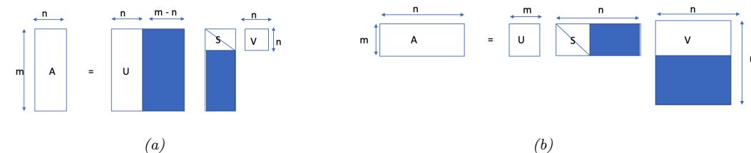
Figure 7.8: SVD decomposition of a matrix, A = USV^T. The shaded parts of each matrix are not computed in the economy-sized version. (a) Tall skinny matrix. (b) Short wide matrix.

where U is an ^{m ↓ m} whose columns are orthornormal (so U^TU = Im), V is ^{n ↓ n} matrix whose rows and columns are orthonormal (so ^VT^{V =} VV^{T = I}n), and ^S is a ^{m ↓ n} matrix containing the r = min(m, n) singular values εⁱ ∋ 0 on the main diagonal, with 0s filling the rest of the matrix. The columns of U are the left singular vectors, and the columns of V are the right singular vectors. This is called the singular value decomposition or SVD of the matrix. See Figure 7.8 for an example.

As is apparent from Figure 7.8a, if m>n, there are at most n singular values, so the last m ↑ n columns of U are irrelevant (since they will be multiplied by 0). The economy sized SVD, also called a thin SVD, avoids computing these unnecessary elements. In other words, if we write the U matrix as U = [U1, U2], we only compute U1. Figure 7.8b shows the opposite case, where m<n, where we represent V = [V1; V2], and only compute V1.

The cost of computing the SVD is O(min(mn², m²n)). Details on how it works can be found in standard linear algebra textbooks.

7.5.2 Connection between SVD and EVD

If A is real, symmetric and positive definite, then the singular values are equal to the eigenvalues, and the left and right singular vectors are equal to the eigenvectors (up to a sign change):

\[\mathbf{A} = \mathbf{U} \mathbf{S} \mathbf{V}^{\overline{\top}} = \mathbf{U} \mathbf{S} \mathbf{U}^{\overline{\top}} = \mathbf{U} \mathbf{S} \mathbf{U}^{-1} \tag{7.179}\]

Note, however, that NumPy always returns the singular values in decreasing order, whereas the eigenvalues need not necessarily be sorted.

In general, for an arbitrary real matrix A, if A = USV^T, we have

\[\mathbf{A}^{\mathsf{T}}\mathbf{A} = \mathbf{V}\mathbf{S}^{\mathsf{T}}\mathbf{U}^{\mathsf{T}}\mathbf{U}\mathbf{S}\mathbf{V}^{\mathsf{T}} = \mathbf{V}(\mathbf{S}^{\mathsf{T}}\mathbf{S})\mathbf{V}^{\mathsf{T}} \tag{7.180}\]

Hence

\[(\mathbf{A}^\top \mathbf{A})\mathbf{V} = \mathbf{V}\mathbf{D}\_n\tag{7.181}\]

so the eigenvectors of A^TA are equal to V, the right singular vectors of A, and the eigenvalues of A^TA are equal to Dⁿ = S^TS, which is an ^{n ↓ n} diagonal matrix containing the squared singular values. Similarly

\[\mathbf{A}\mathbf{A}^{\mathsf{T}} = \mathbf{U}\mathbf{S}\mathbf{V}^{\mathsf{T}} \mathbf{V}\mathbf{S}^{\mathsf{T}}\mathbf{U}^{\mathsf{T}} = \mathbf{U}(\mathbf{S}\mathbf{S}^{\mathsf{T}})\mathbf{U}^{\mathsf{T}} \tag{7.182}\]

\[(\mathbf{A} \mathbf{A}^{\mathsf{T}}) \mathbf{U} = \mathbf{U} \mathbf{D}\_{m} \tag{7.183}\]

so the eigenvectors of AA^T are equal to U, the left singular vectors of A, and the eigenvalues of AA^T are equal to D^m = SS^T, which is an ^{m ↓ m} diagonal matrix containing the squared singular values. In summary,

\[\mathbf{U} = \text{vec}(\mathbf{A}\mathbf{A}^{\mathsf{T}}), \ \mathbf{V} = \text{vec}(\mathbf{A}^{\mathsf{T}}\mathbf{A}), \ \mathbf{D}\_{m} = \text{eval}(\mathbf{A}\mathbf{A}^{\mathsf{T}}), \mathbf{D}\_{n} = \text{eval}(\mathbf{A}^{\mathsf{T}}\mathbf{A})\tag{7.184}\]

If we just use the computed (non-zero) parts in the economy-sized SVD, then we can define

\[\mathbf{D} = \mathbf{S}^2 = \mathbf{S}^\mathsf{T}\mathbf{S} = \mathbf{S}\mathbf{S}^\mathsf{T} \tag{7.185}\]

Note also that an EVD does not always exist, even for square A, whereas an SVD always exists.

7.5.3 Pseudo inverse

The Moore-Penrose pseudo-inverse of A, pseudo inverse denoted A†, is defined as the unique matrix that satisfies the following 4 properties:

\[\mathbf{A}\mathbf{A}^{\dagger}\mathbf{A} = \mathbf{A}, \; \mathbf{A}^{\dagger}\mathbf{A}\mathbf{A}^{\dagger} = \mathbf{A}^{\dagger}, \; (\mathbf{A}\mathbf{A}^{\dagger})^{\top} = \mathbf{A}\mathbf{A}^{\dagger}, \; (\mathbf{A}^{\dagger}\mathbf{A})^{\top} = \mathbf{A}^{\dagger}\mathbf{A} \tag{7.186}\]

If A is square and non-singular, then A† = A→¹.

If m>n (tall, skinny) and the columns of A are linearly independent (so A is full rank), then

\[\mathbf{A}^{\dagger} = (\mathbf{A}^{\top}\mathbf{A})^{-1}\mathbf{A}^{\top} \tag{7.187}\]

which is the same expression as arises in the normal equations (see Section 11.2.2.1). In this case, A† is a left inverse of A because

\[\mathbf{A}^{\dagger}\mathbf{A} = (\mathbf{A}^{\top}\mathbf{A})^{-1}\mathbf{A}^{\dagger}\mathbf{A} = \mathbf{I} \tag{7.188}\]

but is not a right inverse because

\[\mathbf{A}\mathbf{A}^{\dagger} = \mathbf{A}(\mathbf{A}^{\top}\mathbf{A})^{-1}\mathbf{A}^{\top} \tag{7.189}\]

only has rank n, and so cannot be the m ↓ m identity matrix.

If m<n (short, fat) and the rows of A are linearly independent (so A^T is full rank), then the pseudo inverse is

\[\mathbf{A}^{\dagger} = \mathbf{A}^{\top} (\mathbf{A} \mathbf{A}^{\dagger})^{-1} \tag{7.190}\]

In this case, A† is a right inverse of A.

We can compute the pseudo inverse using the SVD decomposition A = USVT. In particular, one can show that

\[\mathbf{A}^{\dagger} = \mathbf{V}[\text{diag}(1/\sigma\_1, \dots, 1/\sigma\_r, 0, \dots, 0)] \mathbf{U}^{\dagger} = \mathbf{V} \mathbf{S}^{-1} \mathbf{U}^{\dagger} \tag{7.191}\]

where r is the rank of the matrix, and where we define S→¹ = diag(ε→^{1 1} ,…, ε→^{1 r} , 0,…, 0). Indeed if the matrices were square and full rank we would have

\[(\mathbf{U}\mathbf{S}\mathbf{V}^{\mathrm{T}})^{-1} = \mathbf{V}\mathbf{S}^{-1}\mathbf{U}^{\mathrm{T}}\tag{7.192}\]

7.5.4 SVD and the range and null space of a matrix *

In this section, we show that the left and right singular vectors form an orthonormal basis for the range and null space.

From Equation (7.178) we have

\[\mathbf{Ax} = \sum\_{j:\sigma\_j>0} \sigma\_j(\mathbf{v}\_j^\mathsf{T} \mathbf{x}) u\_j = \sum\_{j=1}^r \sigma\_j(\mathbf{v}\_j^\mathsf{T} \mathbf{x}) u\_j \tag{7.193}\]

where r is the rank of A. Thus any Ax can be written as a linear combination of the left singular vectors u1,…,ur, so the range of A is given by

\[\text{range}(\mathbf{A}) = \text{span}\left(\{\mathbf{u}\_j : \sigma\_j > 0\}\right) \tag{7.194}\]

with dimension r.

To find a basis for the null space, let us now define a second vector ^{y → Rn} that is a linear combination solely of the right singular vectors for the zero singular values,

\[\mathbf{y} = \sum\_{j:\sigma\_j=0} c\_j \mathbf{v}\_j = \sum\_{j=r+1}^n c\_j \mathbf{v}\_j \tag{7.195}\]

Since the v^j ’s are orthonormal, we have

\[\mathbf{A}\mathbf{y} = \mathbf{U} \begin{pmatrix} \sigma\_1 \mathbf{v}\_1^T \mathbf{y} \\ \vdots \\ \sigma\_r \mathbf{v}\_r^T \mathbf{y} \\ \sigma\_{r+1} \mathbf{v}\_{r+1}^T \mathbf{y} \\ \vdots \\ \sigma\_n \mathbf{v}\_n^T \mathbf{y} \end{pmatrix} = \mathbf{U} \begin{pmatrix} \sigma\_1 \mathbf{0} \\ \vdots \\ \sigma\_r \mathbf{0} \\ \mathbf{0} \mathbf{v}\_{r+1}^T \mathbf{y} \\ \vdots \\ \mathbf{0} \mathbf{v}\_n^T \mathbf{y} \end{pmatrix} = \mathbf{U} \mathbf{0} = \mathbf{0} \tag{7.196}\]

Hence the right singular vectors form an orthonormal basis for the null space:

\[\text{nullspace}(\mathbf{A}) = \text{span}\left(\{\sigma\_j : \sigma\_j = 0\}\right) \tag{7.197}\]

with dimension n ↑ r. We see that

\[ \dim(\text{range}(\mathbf{A})) + \dim(\text{nullspace}(\mathbf{A})) = r + (n - r) = n \tag{7.198} \]

In words, this is often written as

\[\text{rank} + \text{nullity} = n \tag{7.199}\]

This is called the rank-nullity theorem. It follows from this that the rank of a matrix is the number of nonzero singular values.

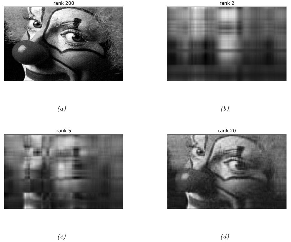
Figure 7.9: Low rank approximations to an image. Top left: The original image is of size 200 → 320, so has rank 200. Subsequent images have ranks 2, 5, and 20. Generated by svd\_image\_demo.ipynb.

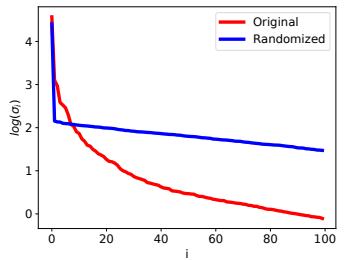
Figure 7.10: First 100 log singular values for the clown image (red line), and for a data matrix obtained by randomly shu#ing the pixels (blue line). Generated by svd\_image\_demo.ipynb. Adapted from Figure 14.24 of [HTF09].

7.5.5 Truncated SVD

Let A = USV^T be the SVD of A, and let Aˆ ^K = UKSKV^{T K}, where we use the first K columns of U and V. This can be shown to be the optimal rank K approximation, in the sense that it minimizes ||^{A ↑ Aˆ K}||² F .

If K = r = rank(A), there is no error introduced by this decomposition. But if K<r, we incur some error. This is called a truncated SVD. If the singular values die o! quickly, as is typical in natural data (see e.g., Figure 7.10), the error will be small. The total number of parameters needed to represent an N ↓ D matrix using a rank K approximation is

\[NK + KD + K = K(N + D + 1)\tag{7.200}\]

As an example, consider the 200 ↓ 320 pixel image in Figure 7.9(top left). This has 64,000 numbers in it. We see that a rank 20 approximation, with only (200 + 320 + 1) ↓ 20 = 10, 420 numbers is a very good approximation.

One can show that the error in this rank-K approximation is given by

\[||\mathbf{A} - \hat{\mathbf{A}}||\_F = \sum\_{k=K+1}^{r} \sigma\_k \tag{7.201}\]

where ε^k is the k’th singular value of A.

7.6 Other matrix decompositions *

In this section, we briefly review some other useful matrix decompositions.

7.6.1 LU factorization

We can factorize any square matrix A into a product of a lower triangular matrix L and an upper triangular matrix U. For example,

\[ \begin{bmatrix} a\_{11} & a\_{12} & a\_{13} \\ a\_{21} & a\_{22} & a\_{23} \\ a\_{31} & a\_{32} & a\_{33} \end{bmatrix} = \begin{bmatrix} l\_{11} & 0 & 0 \\ l\_{21} & l\_{22} & 0 \\ l\_{31} & l\_{32} & l\_{33} \end{bmatrix} \begin{bmatrix} u\_{11} & u\_{12} & u\_{13} \\ 0 & u\_{22} & u\_{23} \\ 0 & 0 & u\_{33} \end{bmatrix} . \tag{7.202} \]

In general we may need to permute the entries in the matrix before creating this decomposition. To see this, suppose a¹¹ = 0. Since a¹¹ = l11u11, this means either l¹¹ or u¹¹ or both must be zero, but that would imply L or U are singular. To avoid this, the first step of the algorithm can simply reorder the rows so that the first element is nonzero. This is repeated for subsequent steps. We can denote this process by

\[\mathbf{PA} = \mathbf{LU} \tag{7.203}\]

where P is a permutation matrix, i.e., a square binary matrix where Pij = 1 if row j gets permuted to row i. This is called partial pivoting.

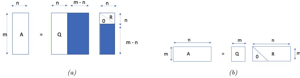
Figure 7.11: Illustration of QR decomposition, A = QR, where Q^TQ = I and R is upper triangular. (a) Tall, skinny matrix. The shaded parts are not computed in the economy-sized version, since they are not needed. (b) Short, wide matrix.

7.6.2 QR decomposition

Suppose we have A ^{→ Rm}↔︎ⁿ representing a set of linearly independent basis vectors (so ^{m ∋ n}), and we want to find a series of orthonormal vectors q1, q2,… that span the successive subspaces of span(a1), span(a1, a2), etc. In other words, we want to find vectors q^j and coe”cients rij such that

\[ \begin{pmatrix} | & | & & | \\ \mathbf{a}\_1 & \mathbf{a}\_2 & \cdots & \mathbf{a}\_n \\ | & | & & | \end{pmatrix} = \begin{pmatrix} | & | & & | \\ \mathbf{q}\_1 & \mathbf{q}\_2 & \cdots & \mathbf{q}\_n \\ | & | & & | \end{pmatrix} \begin{pmatrix} r\_{11} & r\_{12} & \cdots & r\_{1n} \\ r\_{22} & \cdots & r\_{2n} \\ & \ddots & \\ & & r\_{nn} \\ \end{pmatrix} \tag{7.204} \]

We can write this

\[\mathbf{a}\_1 = r\_{11}\mathbf{q}\_1\tag{7.205}\]

\[\mathbf{a}\_2 = r\_{12}\mathbf{q}\_1 + r\_{22}\mathbf{q}\_2\tag{7.206}\]

\[\begin{array}{c} \vdots \\\\ \mathbf{a}\_{n} = r\_{1n}\mathbf{q}\_{1} + \cdots + r\_{nn}\mathbf{q}\_{n} \end{array} \tag{7.207}\]

so we see q¹ spans the space of a1, and q¹ and q² span the space of {a1, a2}, etc.

In matrix notation, we have

\[\mathbf{A} = \hat{\mathbf{Q}} \hat{\mathbf{R}} \tag{7.208}\]

where ^Qˆ is ^{m ↓ n} with orthonormal columns and ^Rˆ is ^{n ↓ n} and upper triangular. This is called a reduced QR or economy sized QR factorization of A; see Figure 7.11.

A full QR factorization appends an additional ^{m ↑ n} orthonormal columns to ^Qˆ so it becomes a square, orthogonal matrix Q, which satisfies QQ^T = QTQ = I. Also, we append rows made of zero to ^Rˆ so it becomes an ^{m ↓ n} matrix that is still upper triangular, called ^R: see Figure 7.11. The zero entries in R “kill o!” the new columns in Q, so the result is the same as Qˆ Rˆ .

QR decomposition is commonly used to solve systems of linear equations, as we discuss in Section 11.2.2.3.

7.6.3 Cholesky decomposition

Any symmetric positive definite matrix can be factorized as A = RTR, where R is upper triangular with real, positive diagonal elements. (This can also be written as A = LL^T, where L = R^T is lower triangular.) This is called a Cholesky factorization or matrix square root. In NumPy, this is implemented by np.linalg.cholesky. The computational complexity of this operation is O(V ³), where V is the number of variables, but can be less for sparse matrices. Below we give some applications of this factorization.

7.6.3.1 Application: Sampling from an MVN

The Cholesky decomposition of a covariance matrix can be used to sample from a multivariate Gaussian. Let ^{y ⇒ N} (µ, !) and ! = LL^T. We first sample ^{x ⇒ N} (0, I), which is easy because it just requires sampling from d separate 1d Gaussians. We then set y = Lx + µ. This is valid since

\[\text{Cov}\left[y\right] = \text{LCov}\left[x\right]\mathbf{L}^{\mathsf{T}} = \mathbf{L}\,\mathbf{I}\,\mathbf{L}^{\mathsf{T}} = \Sigma\]

See cholesky\_demo.ipynb for some code.

7.7 Solving systems of linear equations *

An important application of linear algebra is the study of systems of linear equations. For example, consider the following set of 3 equations:

\[1.3x\_1 + 2x\_2 - x\_3 = 1\tag{7.210}\]

\[2x\_1 - 2x\_2 + 4x\_3 = -2\]

\[-x\_1 + \frac{1}{2}x\_2 - x\_3 = 0\tag{7.212}\]

We can represent this in matrix-vector form as follows:

Ax = b (7.213)

where

\[\mathbf{A} = \begin{pmatrix} 3 & 2 & -1 \\ 2 & -2 & 4 \\ -1 & \frac{1}{2} & -1 \end{pmatrix}, \ b = \begin{pmatrix} 1 \\ -2 \\ 0 \end{pmatrix} \tag{7.214}\]

The solution is x = [1, ↑2, ↑2].

In general, if we have m equations and n unknowns, then A will be a m ↓ n matrix, and b will be a m ↓ 1 vector. If m = n (and A is full rank), there is a single unique solution. If m<n, the system is underdetermined, so there is not a unique solution. If m>n, the system is overdetermined, since there are more constraints than unknowns, and not all the lines intersect at the same point. See Figure 7.12 for an illustration. We discuss how to compute solutions in each of these cases below.

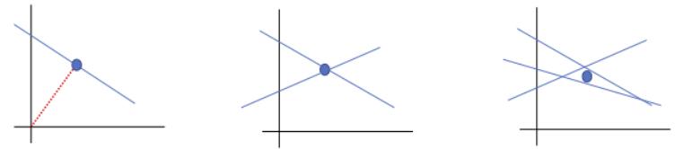
Figure 7.12: Solution of a set of m linear equations in n = 2 variables. (a) m = 1 < n so the system is underdetermined. We show the minimal norm solution as a blue circle. (The dotted red line is orthogonal to the line, and its length is the distance to the origin.) (b) m = n = 2, so there is a unique solution. (c) m = 3 > n, so there is no unique solution. We show the least squares solution.

7.7.1 Solving square systems

In the case where m = n, we can solve for x by computing an LU decomposition, A = LU, and then proceeding as follows:

\[\mathbf{A}x = \mathbf{b} \tag{7.215}\]

\[\mathbf{L}\mathbf{U}x = b\tag{7.216}\]

\[\mathbf{U}x = \mathbf{L}^{-1}\mathbf{b} \stackrel{\Delta}{=} y\]

\[x = \mathbf{U}^{-1}y\tag{7.218}\]

The crucial point is that L and U are both triangular matrices, so we can avoid taking matrix inverses, and use a method known as backsubstitution instead.

In particular, we can solve y = L→¹b without taking inverses as follows. First we write

\[ \begin{pmatrix} L\_{11} \\ L\_{21} & L\_{22} \\ & & \ddots \\ L\_{n1} & L\_{n2} & \cdots & L\_{nn} \end{pmatrix} \begin{pmatrix} y\_1 \\ \vdots \\ y\_n \end{pmatrix} = \begin{pmatrix} b\_1 \\ \vdots \\ b\_n \end{pmatrix} \tag{7.219} \]

We start by solving L11y¹ = b¹ to find y¹ and then substitute this in to solve

\[L\_{21}y\_1 + L\_{22}y\_2 = b\_2\tag{7.220}\]

for y2. We repeat this recursively. This process is often denoted by the backslash operator, ^{y = L  b}. Once we have ^y, we can solve ^{x = U}→^1y using backsubstitution in a similar manner.

7.7.2 Solving underconstrained systems (least norm estimation)

In this section, we consider the underconstrained setting, where m<n. 3 We assume the rows are linearly independent, so A is full rank.

^3. Our presentation is based in part on lecture notes by Stephen Boyd at http://ee263.stanford.edu/lectures/ min-norm.pdf.

When m<n, there are multiple possible solutions, which have the form

\[\{\mathbf{z} : \mathbf{A}\mathbf{z} = \mathbf{b}\} = \{\mathbf{z}\_p + \mathbf{z} : \mathbf{z} \in \text{nullspace}(\mathbf{A})\}\tag{7.221}\]

where x^p is any particular solution. It is standard to pick the particular solution with minimal ω² norm, i.e.,

\[\hat{x} = \operatorname\*{argmin}\_{\mathbf{a}} ||x||\_2^2 \text{ s.t. } \mathbf{A}x = \mathbf{b} \tag{7.222}\]

We can compute the minimal norm solution using the right pseudo inverse:

\[x\_{\rm pinv} = \mathbf{A}^{\rm T} (\mathbf{A} \mathbf{A}^{\rm T})^{-1} \mathbf{b} \tag{7.223}\]

(See Section 7.5.3 for more details.)

To see this, suppose x is some other solution, so Ax = b, and A(x ↑ xpinv) = 0. Thus

\[\mathbf{a}^{\top}(\mathbf{z} - \mathbf{z}\_{\text{pinv}})^{\top}\mathbf{z}\_{\text{pinv}} = (\mathbf{z} - \mathbf{z}\_{\text{pinv}})^{\top}\mathbf{A}^{\top}(\mathbf{A}\mathbf{A}^{\top})^{-1}\mathbf{b} = (\mathbf{A}(\mathbf{z} - \mathbf{z}\_{\text{pinv}}))^{\top}(\mathbf{A}\mathbf{A}^{\top})^{-1}\mathbf{b} = 0\tag{7.224}\]

and hence (x ↑ xpinv) ⇔ xpinv. By Pythagoras’s theorem, the norm of x is

\[||x||^2 = ||x\_{\text{pinv}} + x - x\_{\text{pinv}}||^2 = ||x\_{\text{pinv}}||^2 + ||x - x\_{\text{pinv}}||^2 \ge ||x\_{\text{pinv}}||^2\tag{7.225}\]

Thus any solution apart from xpinv has larger norm.

We can also solve the constrained optimization problem in Equation (7.222) by minimizing the following unconstrained objective

\[\mathcal{L}(\mathbf{x}, \boldsymbol{\lambda}) = \mathbf{x}^{\mathsf{T}} \boldsymbol{x} + \boldsymbol{\lambda}^{\mathsf{T}} (\mathbf{A} \boldsymbol{x} - \mathbf{b}) \tag{7.226}\]

From Section 8.5.1, the optimality conditions are

\[ \nabla\_x \mathcal{L} = 2x + \mathbf{A}^T \lambda = \mathbf{0}, \ \nabla\_\lambda \mathcal{L} = \mathbf{A}x - b = \mathbf{0} \tag{7.227} \]

From the first condition we have ^{x = ↑}A^Tϱ/2. Subsituting into the second we get

\[\mathbf{A}\mathbf{x} = -\frac{1}{2}\mathbf{A}\mathbf{A}^{\top}\boldsymbol{\lambda} = \mathbf{b} \tag{7.228}\]

which implies ^{ϱ = ↑}2(AAT)→¹b. Hence ^{x = A}T(AAT)→¹b, which is the right pseudo inverse solution.

7.7.3 Solving overconstrained systems (least squares estimation)

If m>n, we have an overdetermined solution, which typically does not have an exact solution, but we will try to find the solution that gets as close as possible to satisfying all of the constraints specified by Ax = b. We can do this by minimizing the following cost function, known as the least squares objective: 4

\[f(\mathbf{z}) = \frac{1}{2}||\mathbf{A}\mathbf{z} - \mathbf{b}||\_2^2 \tag{7.233}\]

^4. Note that some equation numbers have been skipped. This is intentional. The reason is that I have omitted some erroneous material from an earlier version (described in https://github.com/probml/pml-book/issues/266), but want to make sure the equation numbering is consistent across di!erent versions of the book.

Using matrix calculus results from Section 7.8 we have that the gradient is given by

\[\mathbf{g}(\mathbf{x}) = \frac{\partial}{\partial \mathbf{x}} f(\mathbf{x}) = \mathbf{A}^{\mathsf{T}} \mathbf{A} \mathbf{x} - \mathbf{A}^{\mathsf{T}} \mathbf{b} \tag{7.234}\]

The optimum can be found by solving g(x) = 0. This gives

\[\mathbf{A}^{\top}\mathbf{A}x = \mathbf{A}^{\top}\mathbf{b} \tag{7.235}\]

These are known as the normal equations, since, at the optimal solution, b ↑ Ax is normal (orthogonal) to the range of A, as we explain in Section 11.2.2.2. The corresponding solution xˆ is the ordinary least squares (OLS) solution, which is given by

\[ \hat{x} = (\mathbf{A}^{\mathsf{T}} \mathbf{A})^{-1} \mathbf{A}^{\mathsf{T}} \mathbf{b} \tag{7.236} \]

The quantity A† = (A^TA)→¹A^T is the left pseudo inverse of the (non-square) matrix A (see Section 7.5.3 for more details).

We can check that the solution is unique by showing that the Hessian is positive definite. In this case, the Hessian is given by

\[\mathbf{H}(\mathbf{x}) = \frac{\partial^2}{\partial x^2} f(\mathbf{x}) = \mathbf{A}^\mathsf{T} \mathbf{A} \tag{7.237}\]

If A is full rank (so the columns of A are linearly independent), then H is positive definite, since for any v > 0, we have

\[\mathbf{v}^{\mathsf{T}}(\mathbf{A}^{\mathsf{T}}\mathbf{A})\mathbf{v} = (\mathbf{A}\mathbf{v})^{\mathsf{T}}(\mathbf{A}\mathbf{v}) = ||\mathbf{A}\mathbf{v}||^{2} > 0\tag{7.238}\]

Hence in the full rank case, the least squares objective has a unique global minimum.

7.8 Matrix calculus

The topic of calculus concerns computing “rates of change” of functions as we vary their inputs. It is of vital importance to machine learning, as well as almost every other numerical discipline. In this section, we review some standard results. In some cases, we use some concepts and notation from matrix algebra, which we cover in Chapter 7. For more details on these results from a deep learning perspective, see [PH18].

7.8.1 Derivatives

Consider a scalar-argument function f : R ↔︎ R. We define its derivative at a point x to be the quantity

\[f'(x) \triangleq \lim\_{h \to 0} \frac{f(x+h) - f(x)}{h} \tag{7.239}\]

assuming the limit exists. This measures how quickly the output changes when we move a small distance in input space away from x (i.e., the “rate of change” of the function). We can interpret f↗ (x) as the slope of the tangent line at f(x), and hence

\[f(x+h) \approx f(x) + f'(x)h\tag{7.240}\]

for small h.

We can compute a finite di”erence approximation to the derivative by using a finite step size h, as follows:

\[f'(x) = \underbrace{\lim\_{h \to 0} \frac{f(x+h) - f(x)}{h}}\_{\text{forward difference}} = \underbrace{\lim\_{h \to 0} \frac{f(x+h/2) - f(x-h/2)}{h}}\_{\text{central difference}} = \underbrace{\lim\_{h \to 0} \frac{f(x) - f(x-h)}{h}}\_{\text{backward difference}} \tag{7.241}\]

The smaller the step size h, the better the estimate, although if h is too small, there can be errors due to numerical cancellation.

We can think of di!erentiation as an operator that maps functions to functions, D(f) = f↗ , where f↗ (x) computes the derivative at x (assuming the derivative exists at that point). The use of the prime symbol f↗ to denote the derivative is called Lagrange notation. The second derivative function, which measures how quickly the gradient is changing, is denoted by f↗↗. The n’th derivative function is denoted f(n) .

Alternatively, we can use Leibniz notation, in which we denote the function by y = f(x), and its derivative by dy dx or ^d dx ^f(x). To denote the evaluation of the derivative at a point ^a, we write df dx x=a .

7.8.2 Gradients

We can extend the notion of derivatives to handle vector-argument functions, ^f : ^{Rn ↔︎ R}, by defining the partial derivative of f with respect to xⁱ to be

\[\frac{\partial f}{\partial x\_i} = \lim\_{h \to 0} \frac{f(x + h\mathbf{e}\_i) - f(x)}{h} \tag{7.242}\]

where eⁱ is the i’th unit vector.

The gradient of a function at a point x is the vector of its partial derivatives:

\[\mathbf{g} = \frac{\partial f}{\partial x} = \nabla f = \begin{pmatrix} \frac{\partial f}{\partial x\_1} \\ \vdots \\ \frac{\partial f}{\partial x\_n} \end{pmatrix} \tag{7.243}\]

To emphasize the point at which the gradient is evaluated, we can write

\[\left.g(x^\*)\right| \triangleq \frac{\partial f}{\partial x}\bigg|\_{x^\*}\tag{7.244}\]

We see that the operator ̸ (pronounced “nabla”) maps a function ^f : ^{Rn ↔︎ R} to another function ^g : ^{Rn ↔︎ Rn}. Since ^g() is a vector-valued function, it is known as a vector field. By contrast, the derivative function f↗ is a scalar field.

7.8.3 Directional derivative

The directional derivative measures how much the function ^f : ^{Rn ↔︎ R} changes along a direction v in space. It is defined as follows

\[D\_{\mathbf{v}}f(\mathbf{z}) = \lim\_{h \to 0} \frac{f(\mathbf{z} + h\mathbf{v}) - f(\mathbf{z})}{h} \tag{7.245}\]

We can approximate this numerically using 2 function calls to f, regardless of n. By contrast, a numerical approximation to the standard gradient vector takes n + 1 calls (or 2n if using central di!erences).

Note that the directional derivative along v is the scalar product of the gradient g and the vector v:

\[D\_v f(x) = \nabla f(x) \cdot v\]

7.8.4 Total derivative *

Suppose that some of the arguments to the function depend on each other. Concretely, suppose the function has the form f(t, x(t), y(t)). We define the total derivative of f wrt t as follows:

\[\frac{df}{dt} = \frac{\partial f}{\partial t} + \frac{\partial f}{\partial x}\frac{dx}{dt} + \frac{\partial f}{\partial y}\frac{dy}{dt} \tag{7.247}\]

If we multiply both sides by the di!erential dt, we get the total di”erential

\[df = \frac{\partial f}{\partial t}dt + \frac{\partial f}{\partial x}dx + \frac{\partial f}{\partial y}dy\tag{7.248}\]

This measures how much f changes when we change t, both via the direct e!ect of t on f, but also indirectly, via the e!ects of t on x and y.

7.8.5 Jacobian

Consider a function that maps a vector to another vector, ^f : ^{Rn ↔︎ Rm}. The Jacobian matrix of this function is an m ↓ n matrix of partial derivatives:

\[\mathbf{J}\_f(\mathbf{z}) = \frac{\partial f}{\partial \mathbf{z}^\mathsf{T}} \stackrel{\scriptstyle \triangleq}{=} \begin{pmatrix} \frac{\partial f\_1}{\partial x\_1} & \cdots & \frac{\partial f\_1}{\partial x\_n} \\ \vdots & \ddots & \vdots \\ \frac{\partial f\_m}{\partial x\_1} & \cdots & \frac{\partial f\_m}{\partial x\_n} \end{pmatrix} = \begin{pmatrix} \nabla f\_1(\mathbf{z})^\mathsf{T} \\ \vdots \\ \nabla f\_m(\mathbf{z})^\mathsf{T} \end{pmatrix} \tag{7.249}\]

Note that we lay out the results in the same orientation as the output f; this is sometimes called numerator layout or the Jacobian formulation.5

7.8.5.1 Multiplying Jacobians and vectors

The Jacobian vector product or JVP is defined to be the operation that corresponds to rightmultiplying the Jacobian matrix ^{J → Rm}↔︎ⁿ by a vector ^{v → Rn}:

\[\mathbf{J}\_f(\mathbf{z})\mathbf{v} = \begin{pmatrix} \nabla f\_1(\mathbf{z})^\mathsf{T} \\ \vdots \\ \nabla f\_m(\mathbf{z})^\mathsf{T} \end{pmatrix} \mathbf{v} = \begin{pmatrix} \nabla f\_1(\mathbf{z})^\mathsf{T}\mathbf{v} \\ \vdots \\ \nabla f\_m(\mathbf{z})^\mathsf{T}\mathbf{v} \end{pmatrix} \tag{7.250}\]

^5. For a much more detailed discussion of notation, see https://en.wikipedia.org/wiki/Matrix\_calculus.

So we can see that we can approximate this numerically using just 2 calls to f.

The vector Jacobian product or VJP is defined to be the operation that corresponds to left-multiplying the Jacobian matrix ^{J → R}m↔︎ⁿ by a vector ^{u → R}m:

\[\mathbf{u}^{\mathsf{T}} \mathbf{J}\_{f}(\mathbf{z}) = \mathbf{u}^{\mathsf{T}} \left( \frac{\partial f}{\partial x\_{1}}, \dots, \frac{\partial f}{\partial x\_{n}} \right) = \left( \mathbf{u} \cdot \frac{\partial f}{\partial x\_{1}}, \dots, \mathbf{u} \cdot \frac{\partial f}{\partial x\_{n}} \right) \tag{7.251}\]

The JVP is more e”cient if m ∋ n, and the VJP is more e”cient if m ↘ n. See Section 13.3 for details on how this can be used to perform automatic di!erentiation in a computation graph such as a DNN.

7.8.5.2 Jacobian of a composition

Sometimes it is useful to take the Jacobian of the composition of two functions. Let h(x) = g(f(x)). By the chain rule of calculus, we have

\[\mathbf{J}\_h(x) = \mathbf{J}\_g(f(x))\mathbf{J}\_f(x) \tag{7.252}\]

For example, suppose ^f : ^{R ↔︎ R2} and ^g : ^{R2 ↔︎ R2}. We have

\[\frac{\partial \mathbf{g}}{\partial x} = \begin{pmatrix} \frac{\partial}{\partial x} g\_1(f\_1(x), f\_2(x)) \\ \frac{\partial}{\partial x} g\_2(f\_1(x), f\_2(x)) \end{pmatrix} = \begin{pmatrix} \frac{\partial g\_1}{\partial f\_1} \frac{\partial f\_1}{\partial x} + \frac{\partial g\_1}{\partial f\_2} \frac{\partial f\_2}{\partial x} \\ \frac{\partial g\_2}{\partial f\_1} \frac{\partial f\_1}{\partial x} + \frac{\partial g\_2}{\partial f\_2} \frac{\partial f\_2}{\partial x} \end{pmatrix} \tag{7.253}\]

\[\mathbf{f} = \frac{\partial \mathbf{g}}{\partial \mathbf{f}^{\mathsf{T}}} \frac{\partial \mathbf{f}}{\partial x} = \begin{pmatrix} \frac{\partial g\_1}{\partial f\_1} & \frac{\partial g\_1}{\partial f\_2} \\ \frac{\partial g\_2}{\partial f\_1} & \frac{\partial g\_2}{\partial f\_2} \end{pmatrix} \begin{pmatrix} \frac{\partial f\_1}{\partial x} \\ \frac{\partial f\_2}{\partial x} \end{pmatrix} \tag{7.254}\]

7.8.6 Hessian

For a function ^f : ^{Rn ↔︎ R} that is twice di!erentiable, we define the Hessian matrix as the (symmetric) n ↓ n matrix of second partial derivatives:

\[\mathbf{H}\_f = \frac{\partial^2 f}{\partial x^2} = \nabla^2 f = \begin{pmatrix} \frac{\partial^2 f}{\partial x\_1^2} & \cdots & \frac{\partial^2 f}{\partial x\_1 \partial x\_n} \\ & \vdots \\ \frac{\partial^2 f}{\partial x\_n \partial x\_1} & \cdots & \frac{\partial^2 f}{\partial x\_n^2} \end{pmatrix} \tag{7.255}\]

We see that the Hessian is the Jacobian of the gradient.

7.8.7 Gradients of commonly used functions

In this section, we list without proof the gradients of certain widely used functions.

7.8.7.1 Functions that map scalars to scalars

Consider a di!erentiable function f : R ↔︎ R. Here are some useful identities from scalar calculus, which you should already be familiar with.

\[\frac{d}{dx}cx^n = cnx^{n-1} \tag{7.256}\]

\[\frac{d}{dx}\log(x) = 1/x \tag{7.257}\]

\[\frac{d}{dx}\exp(x) = \exp(x)\tag{7.258}\]

\[\frac{d}{dx}\left[f(x) + g(x)\right] = \frac{df(x)}{dx} + \frac{dg(x)}{dx} \tag{7.259}\]

\[\frac{d}{dx}\left[f(x)g(x)\right] = f(x)\frac{dg(x)}{dx} + g(x)\frac{df(x)}{dx} \tag{7.260}\]

\[\frac{d}{dx}f(u(x)) = \frac{du}{dx}\frac{df(u)}{du} \tag{7.261}\]

Equation (7.261) is known as the chain rule of calculus.

7.8.7.2 Functions that map vectors to scalars

Consider a di!erentiable function ^f : ^{Rn ↔︎ R}. Here are some useful identities:6

\[\frac{\partial (\mathbf{a}^{\mathsf{T}} \mathbf{x})}{\partial \mathbf{x}} = \mathbf{a}\]

\[\frac{\partial(\mathbf{b}^{\mathsf{T}}\mathbf{A}\mathbf{x})}{\partial x} = \mathbf{A}^{\mathsf{T}}\mathbf{b}\]

\[\frac{\partial (\mathbf{x}^{\mathsf{T}} \mathbf{A} \mathbf{x})}{\partial \mathbf{x}} = (\mathbf{A} + \mathbf{A}^{\mathsf{T}}) \mathbf{x} \tag{7.264}\]

It is fairly easy to prove these identities by expanding out the quadratic form, and applying scalar calculus.

7.8.7.3 Functions that map matrices to scalars

Consider a function ^f : ^Rm↔︎^{n ↔︎ R} which maps a matrix to a scalar. We are using the following natural layout for the derivative matrix:

\[\frac{\partial f}{\partial \mathbf{X}} = \begin{pmatrix} \frac{\partial f}{\partial x\_{11}} & \cdots & \frac{\partial f}{\partial x\_{1n}} \\ & \vdots \\ \frac{\partial f}{\partial x\_{m1}} & \cdots & \frac{\partial f}{\partial x\_{mn}} \end{pmatrix} \tag{7.265}\]

Below are some useful identities.

^6. Some of the identities are taken from the list at http://www.cs.nyu.edu/~roweis/notes/matrixid.pdf.

Identities involving quadratic forms

One can show the following results.

\[\begin{aligned} \frac{\partial}{\partial \mathbf{X}} (\mathbf{a}^{\mathsf{T}} \mathbf{X} \mathbf{b}) &= \mathbf{a} \mathbf{b}^{\mathsf{T}} \\ \frac{\partial}{\partial \mathbf{X}} (\mathbf{a}^{\mathsf{T}} \mathbf{X}^{\mathsf{T}} \mathbf{b}) &= \mathbf{b} \mathbf{a}^{\mathsf{T}} \end{aligned} \tag{7.266}\]

Identities involving matrix trace

One can show the following results.

\[\frac{\partial}{\partial \mathbf{X}} \text{tr}(\mathbf{A} \mathbf{X} \mathbf{B}) = \mathbf{A}^{\mathsf{T}} \mathbf{B}^{\mathsf{T}} \tag{7.268}\]

\[\frac{\partial}{\partial \mathbf{X}} \text{tr}(\mathbf{X}^{\mathsf{T}} \mathbf{A}) = \mathbf{A}\]

\[\frac{\partial}{\partial \mathbf{X}} \text{tr}(\mathbf{X}^{-1} \mathbf{A}) = -\mathbf{X}^{-\mathsf{T}} \mathbf{A}^{\mathsf{T}} \mathbf{X}^{-\mathsf{T}} \tag{7.270}\]

\[\frac{\partial}{\partial \mathbf{X}} \text{tr}(\mathbf{X}^{\mathsf{T}} \mathbf{A} \mathbf{X}) = (\mathbf{A} + \mathbf{A}^{\mathsf{T}}) \mathbf{X} \tag{7.271}\]

Identities involving matrix determinant

One can show the following results.

\[\frac{\partial}{\partial \mathbf{X}} \det(\mathbf{A} \mathbf{X} \mathbf{B}) = \det(\mathbf{A} \mathbf{X} \mathbf{B}) \mathbf{X}^{-\mathsf{T}} \tag{7.272}\]

\[\frac{\partial}{\partial \mathbf{X}} \log(\det(\mathbf{X})) = \mathbf{X}^{-\mathsf{T}} \tag{7.273}\]

7.9 Exercises

Exercise 7.1 [Orthogonal matrices]

1. A rotation in 3d by angle ω about the z axis is given by the following matrix:

\[\mathbf{R}(\alpha) = \begin{pmatrix} \cos(\alpha) & -\sin(\alpha) & 0 \\ \sin(\alpha) & \cos(\alpha) & 0 \\ 0 & 0 & 1 \end{pmatrix} \tag{7.274}\]

Prove that R is an orthogonal matrix, i.e., R^T R = I, for any ω.

2. What is the only eigenvector ^v of ^R with an eigenvalue of 1.0 and of unit norm (i.e., ||v||² = 1)? (Your answer should be the same for any ω.) Hint: think about the geometrical interpretation of eigenvectors.

Exercise 7.2 [Eigenvectors by hand † ]

Find the eigenvalues and eigenvectors of the following matrix

\[A = \begin{pmatrix} 2 & 0 \\ 0 & 3 \end{pmatrix} \tag{7.275}\]

Compute your result by hand and check it with Python.

8 Optimization

Parts of this chapter were written by Frederik Kunstner, Si Yi Meng, Aaron Mishkin, Sharan Vaswani, and Mark Schmidt.

8.1 Introduction

We saw in Chapter 4 that the core problem in machine learning is parameter estimation (aka model fitting). This requires solving an optimization problem, where we try to find the values for a set of variables ω → #, that minimize a scalar-valued loss function or cost function L : # ↔︎ R:

\[\theta^\* \in \operatorname\*{argmin}\_{\theta \in \Theta} \mathcal{L}(\theta) \tag{8.1}\]

We will assume that the parameter space is given by # ′ ^RD, where ^D is the number of variables being optimized over. Thus we are focusing on continuous optimization, rather than discrete optimization.

If we want to maximize a score function or reward function R(ω), we can equivalently minimize L(ω) = ↑R(ω). We will use the term objective function to refer generically to a function we want to maximize or minimize. An algorithm that can find an optimum of an objective function is often called a solver.

In the rest of this chapter, we discuss di!erent kinds of solvers for di!erent kinds of objective functions, with a focus on methods used in the machine learning community. For more details on optimization, please consult some of the many excellent textbooks, such as [KW19b; BV04; NW06; Ber15; Ber16] as well as various review articles, such as [BCN18; Sun+19b; PPS18; Pey20]. A visualization of the taxonomy of optimization algorithms can be found at https://neos-guide. org/guide/types.

8.1.1 Local vs global optimization

A point that satisfies Equation (8.1) is called a global optimum. Finding such a point is called global optimization.

In general, finding global optima is computationally intractable [Neu04]. In such cases, we will just try to find a local optimum. For continuous problems, this is defined to be a point ω^↓ which has lower (or equal) cost than “nearby” points. Formally, we say ω^↓ is a local minimum if

\[\exists \delta > 0, \,\forall \theta \in \Theta \text{ s.t. } ||\theta - \theta^\*|| < \delta, \,\mathcal{L}(\theta^\*) \le \mathcal{L}(\theta) \tag{8.2}\]

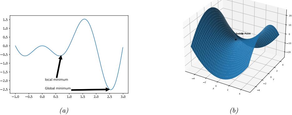
Figure 8.1: (a) Illustration of local and global minimum in 1d. Generated by extrema\_fig\_1d.ipynb. (b) Illustration of a saddle point in 2d. Generated by saddle.ipynb.

A local minimum could be surrounded by other local minima with the same objective value; this is known as a flat local minimum. A point is said to be a strict local minimum if its cost is strictly lower than those of neighboring points:

\[\exists \delta > 0, \forall \theta \in \Theta, \theta \neq \theta^\* : ||\theta - \theta^\*|| < \delta, \mathcal{L}(\theta^\*) < \mathcal{L}(\theta) \tag{8.3}\]

We can define a (strict) local maximum analogously. See Figure 8.1a for an illustration.

A final note on terminology; if an algorithm is guaranteed to converge to a stationary point from any starting point, it is called globally convergent. However, this does not mean (rather confusingly) that it will converge to a global optimum; instead, it just means it will converge to some stationary point.

8.1.1.1 Optimality conditions for local vs global optima

For continuous, twice di!erentiable functions, we can precisely characterize the points which correspond to local minima. Let ^g(ω) = ̸L(ω) be the gradient vector, and H(ω) = ̸²L(ω) be the Hessian matrix. (See Section 7.8 for a refresher on these concepts, if necessary.) Consider a point ^{ω↓ → RD}, and let ^{g↓ = g}(ω)|^ω↑ be the gradient at that point, and ^{H↓ = H}(ω)|^ω↑ be the corresponding Hessian. One can show that the following conditions characterize every local minimum:

• Necessary condition: If ω^↓ is a local minimum, then we must have g^↓ = 0 (i.e., ω^↓ must be a stationary point), and H^↓ must be positive semi-definite.
• Su”cient condition: If g^↓ = 0 and H^↓ is positive definite, then ω^↓ is a local optimum.

To see why the first condition is necessary, suppose we were at a point ω^↓ at which the gradient is non-zero: at such a point, we could decrease the function by following the negative gradient a small distance, so this would not be optimal. So the gradient must be zero. (In the case of nonsmooth

.

functions, the necessary condition is that the zero is a local subgradient at the minimum.) To see why a zero gradient is not su”cient, note that the stationary point could be a local minimum, maximum or saddle point, which is a point where some directions point downhill, and some uphill (see Figure 8.1b). More precisely, at a saddle point, the eigenvalues of the Hessian will be both positive and negative. However, if the Hessian at a point is positive semi-definite, then some directions may point uphill, while others are flat. Moreover, if the Hessian is strictly positive definite, then we are at the bottom of a “bowl”, and all directions point uphill, which is su”cient for this to be a minimum.

8.1.2 Constrained vs unconstrained optimization

In unconstrained optimization, we define the optimization task as finding any value in the parameter space # that minimizes the loss. However, we often have a set of constraints on the allowable values. It is standard to partition the set of constraints C into inequality constraints, g^j (ω) ↘ 0 for j → I and equality constraints, hk(ω)=0 for k → E. For example, we can represent a sum-to-one constraint as an equality constraint ^h(ω) = (1↑$^{D i}=1 ϖi)=0, and we can represent a nonnegativity constraint on the parameters by using D inequality constraints of the form gi(ω) = ↑ϖⁱ ↘ 0

We define the feasible set as the subset of the parameter space that satisfies the constraints:

\[\mathcal{C} = \{\theta : g\_j(\theta) \le 0 : j \in \mathcal{Z}, h\_k(\theta) = 0 : k \in \mathcal{E}\} \subseteq \mathbb{R}^D \tag{8.4}\]

Our constrained optimization problem now becomes

\[\theta^\* \in \operatorname\*{argmin}\_{\theta \in \mathcal{C}} \mathcal{L}(\theta) \tag{8.5}\]

If ^{C = RD}, it is called unconstrained optimization.

The addition of constraints can change the number of optima of a function. For example, a function that was previously unbounded (and hence had no well-defined global maximum or minimum) can “acquire” multiple maxima or minima when we add constraints, as illustrated in Figure 8.2. However, if we add too many constraints, we may find that the feasible set becomes empty. The task of finding any point (regardless of its cost) in the feasible set is called a feasibility problem; this can be a hard subproblem in itself.

A common strategy for solving constrained problems is to create penalty terms that measure how much we violate each constraint. We then add these terms to the objective and solve an unconstrained optimization problem. The Lagrangian is a special case of such a combined objective (see Section 8.5 for details).

8.1.3 Convex vs nonconvex optimization

In convex optimization, we require the objective to be a convex function defined over a convex set (we define these terms below). In such problems, every local minimum is also a global minimum. Thus many models are designed so that their training objectives are convex.

8.1.3.1 Convex sets

We say S is a convex set if, for any x, x↗ → S, we have

\[ \lambda x + (1 - \lambda)x' \in \mathcal{S}, \ \forall \ \lambda \in [0, 1] \tag{8.6} \]

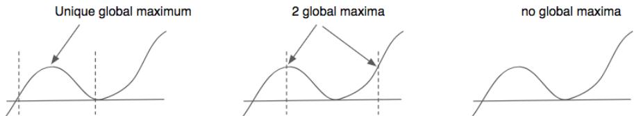
Figure 8.2: Illustration of constrained maximization of a nonconvex 1d function. The area between the dotted vertical lines represents the feasible set. (a) There is a unique global maximum since the function is concave within the support of the feasible set. (b) There are two global maxima, both occuring at the boundary of the feasible set. (c) In the unconstrained case, this function has no global maximum, since it is unbounded.

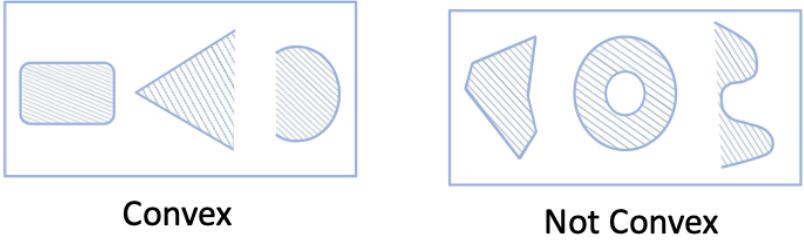
Figure 8.3: Illustration of some convex and non-convex sets.

That is, if we draw a line from x to x↗ , all points on the line lie inside the set. See Figure 8.3 for some illustrations of convex and non-convex sets.

8.1.3.2 Convex functions

We say f is a convex function if its epigraph (the set of points above the function, illustrated in Figure 8.4a) defines a convex set. Equivalently, a function f(x) is called convex if it is defined on a convex set and if, for any x, y → S, and for any 0 ↘ φ ↘ 1, we have

\[f(\lambda x + (1 - \lambda)y) \le \lambda f(x) + (1 - \lambda)f(y) \tag{8.7}\]

See Figure 8.5(a) for a 1d example of a convex function. A function is called strictly convex if the inequality is strict. A function f(x) is concave if ↑f(x) is convex, and strictly concave if ↑f(x) is strictly convex. See Figure 8.5(b) for a 1d example of a function that is neither convex nor concave.

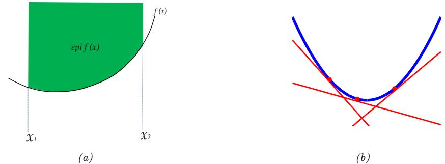
Figure 8.4: (a) Illustration of the epigraph of a function. (b) For a convex function f(x), its epipgraph can be represented as the intersection of half-spaces defined by linear lower bounds derived from the conjugate function f ^↔︎(↼) = max^x ↼x ↑ f(x).

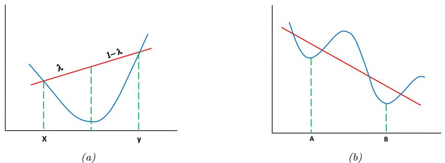
Figure 8.5: (a) Illustration of a convex function. We see that the chord joining (x, f(x)) to (y, f(y)) lies above the function. (b) A function that is neither convex nor concave. A is a local minimum, B is a global minimum.

Here are some examples of 1d convex functions:

x2 eax ↑ log x x^a, a> 1,x> 0 |x| ^a, a ^{∋ 1} x log x, x > 0

8.1.3.3 Characterization of convex functions

Intuitively, a convex function is shaped like a bowl. Formally, one can prove the following important result:

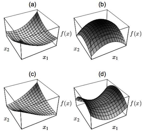
Figure 8.6: The quadratic form f(x) = x^TAx in 2d. (a) A is positive definite, so f is convex. (b) A is negative definite, so f is concave. (c) A is positive semidefinite but singular, so f is convex, but not strictly. Notice the valley of constant height in the middle. (d) A is indefinite, so f is neither convex nor concave. The stationary point in the middle of the surface is a saddle point. From Figure 5 of [She94].

Theorem 8.1.1. Suppose ^f : ^{Rn ↔︎ R} is twice di!erentiable over its domain. Then ^f is convex i! ^{H =} ̸²f(x) is positive semi definite (Section 7.1.5.3) for all ^{x →} dom(f). Furthermore, ^f is strictly convex if H is positive definite.

For example, consider the quadratic form

\[f(\mathbf{x}) = \mathbf{x}^{\mathsf{T}} \mathbf{A} \mathbf{x} \tag{8.8}\]

This is convex if A is positive semi definite, and is strictly convex if A is positive definite. It is neither convex nor concave if A has eigenvalues of mixed sign. See Figure 8.6.

8.1.3.4 Strongly convex functions

We say a function f is strongly convex with parameter m > 0 if the following holds for all x, y in f’s domain:

\[m\left(\nabla f(\mathbf{x}) - \nabla f(\mathbf{y})\right)^{\mathsf{T}}(\mathbf{x} - \mathbf{y}) \ge m||\mathbf{x} - \mathbf{y}||\_2^2 \tag{8.9}\]

A strongly convex function is also strictly convex, but not vice versa.

If the function f is twice continuously di!erentiable, then it is strongly convex with parameter m if and only if ̸²f(x) ^{ℵ mI} for all ^x in the domain, where ^I is the identity and ̸^2f is the Hessian matrix, and the inequality ^ℵ means that ̸²f(x) ^{↑ m}I is positive semi-definite. This is equivalent

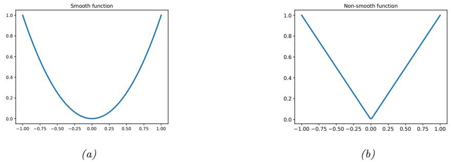
Figure 8.7: (a) Smooth 1d function. (b) Non-smooth 1d function. (There is a discontinuity at the origin.) Generated by smooth-vs-nonsmooth-1d.ipynb.

to requiring that the minimum eigenvalue of ̸²f(x) be at least ^m for all ^x. If the domain is just the real line, then ̸²f(x) is just the second derivative ^f↗↗(x), so the condition becomes ^f↗↗(x) ^{∋ m}. If m = 0, then this means the Hessian is positive semidefinite (or if the domain is the real line, it means that f↗↗(x) ∋ 0), which implies the function is convex, and perhaps strictly convex, but not strongly convex.

The distinction between convex, strictly convex, and strongly convex is rather subtle. To better understand this, consider the case where f is twice continuously di!erentiable and the domain is the real line. Then we can characterize the di!erences as follows:

• f is convex if and only if f↗↗(x) ∋ 0 for all x.
• f is strictly convex if f↗↗(x) > 0 for all x (note: this is su”cient, but not necessary).
• f is strongly convex if and only if f↗↗(x) ∋ m > 0 for all x.

Note that it can be shown that a function f is strongly convex with parameter m i! the function

\[J(x) = f(x) - \frac{m}{2}||x||^2\tag{8.10}\]

is convex.

8.1.4 Smooth vs nonsmooth optimization

In smooth optimization, the objective and constraints are continuously di!erentiable functions. For smooth functions, we can quantify the degree of smoothness using the Lipschitz constant. In the 1d case, this is defined as any constant L ∋ 0 such that, for all real x¹ and x2, we have

\[|f(x\_1) - f(x\_2)| \le L|x\_1 - x\_2|\tag{8.11}\]

This is illustrated in Figure 8.8: for a given constant L, the function output cannot change by more than L if we change the function input by 1 unit. This can be generalized to vector inputs using a suitable norm.

In nonsmooth optimization, there are at least some points where the gradient of the objective function or the constraints is not well-defined. See Figure 8.7 for an example. In some optimization

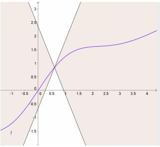
Figure 8.8: For a Lipschitz continuous function f, there exists a double cone (white) whose origin can be moved along the graph of f so that the whole graph always stays outside the double cone. From https: // en. wikipedia. org/ wiki/ Lipschitz\_ continuity . Used with kind permission of Wikipedia author Taschee.

problems, we can partition the objective into a part that only contains smooth terms, and a part that contains the nonsmooth terms:

\[ \mathcal{L}(\boldsymbol{\theta}) = \mathcal{L}\_s(\boldsymbol{\theta}) + \mathcal{L}\_r(\boldsymbol{\theta}) \tag{8.12} \]

where L^s is smooth (di!erentiable), and L^r is nonsmooth (“rough”). This is often referred to as a composite objective. In machine learning applications, L^s is usually the training set loss, and L^r is a regularizer, such as the ω¹ norm of ω. This composite structure can be exploited by various algorithms.

8.1.4.1 Subgradients

In this section, we generalize the notion of a derivative to work with functions which have local discontinuities. In particular, for a convex function of several variables, ^f : ^{Rn ↔︎ R}, we say that ^{g → Rn} is a subgradient of ^f at ^{x →} dom(f) if for all ^{z →} dom(f),

\[f(\mathbf{z}) \ge f(\mathbf{z}) + \mathbf{g}^{\mathsf{T}}(\mathbf{z} - \mathbf{z}) \tag{8.13}\]

Note that a subgradient can exist even when f is not di!erentiable at a point, as shown in Figure 8.9.

A function f is called subdi”erentiable at x if there is at least one subgradient at x. The set of such subgradients is called the subdi”erential of f at x, and is denoted 0f(x).

For example, consider the absolute value function f(x) = |x|. Its subdi!erential is given by

\[\partial f(x) = \begin{cases} \{-1\} & \text{if } x < 0\\ \begin{bmatrix} -1, 1 \end{bmatrix} & \text{if } x = 0\\ \{+1\} & \text{if } x > 0 \end{cases} \tag{8.14}\]

where the notation [↑1, 1] means any value between -1 and 1 inclusive. See Figure 8.10 for an illustration.

8.2 First-order methods

In this section, we consider iterative optimization methods that leverage first-order derivatives of the objective function, i.e., they compute which directions point “downhill”, but they ignore curvature

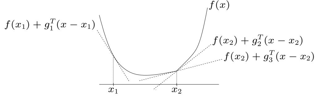
Subgradient of a function

^f(y) ^{≥ f}(x) + ^gT (^{y − x}) for all ^y

g is a subgradient of f (not necessarily convex) at x if

g2, g³ are subgradients at x2; g¹ is a subgradient at x¹ EE364b, Stanford University 2 Figure 8.9: Illustration of subgradients. At x1, the convex function f is di!erentiable, and g¹ (which is the derivative of f at x1) is the unique subgradient at x1. At the point x2, f is not di!erentiable, because of the “kink”. However, there are many subgradients at this point, of which two are shown. From https: // web. stanford. edu/ class/ ee364b/ lectures/ subgradients\_ slides. pdf . Used with kind permission of Stephen Boyd. Example f(x) = |x|

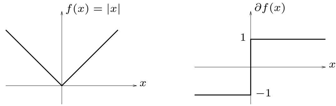
righthand plot shows ! {(x, g) ^{| x ∈ R}, g ^{∈ ∂}f(x)} Figure 8.10: The absolute value function (left) and its subdi!erential (right). From https: // web. stanford. edu/ class/ ee364b/ lectures/ subgradients\_ slides. pdf . Used with kind permission of Stephen Boyd.

information. All of these algorithms require that the user specify a starting point ω0. Then at each iteration t, they perform an update of the following form:

\[ \theta\_{t+1} = \theta\_t + \eta\_t \mathbf{d}\_t \tag{8.15} \]

where ◁^t is known as the step size or learning rate, and d^t is a descent direction, such as the negative of the gradient, given by g^t = ̸ωL(ω)|^ωt . These update steps are continued until the method reaches a stationary point, where the gradient is zero.

8.2.1 Descent direction

We say that a direction d is a descent direction if there is a small enough (but nonzero) amount ◁ we can move in direction d and be guaranteed to decrease the function value. Formally, we require that there exists an ◁max > 0 such that

\[ \mathcal{L}(\theta + \eta \mathbf{d}) < \mathcal{L}(\theta) \tag{8.16} \]

for all 0 < ◁ < ◁max. The gradient at the current iterate, ωt, is given by

\[\mathcal{g}\_t \triangleq \nabla \mathcal{L}(\boldsymbol{\theta})|\_{\boldsymbol{\theta}\_t} = \nabla \mathcal{L}(\boldsymbol{\theta}\_t) = \mathbf{g}(\boldsymbol{\theta}\_t) \tag{8.17}\]

This points in the direction of maximal increase in f, so the negative gradient is a descent direction. It can be shown that any direction d is also a descent direction if the angle ϖ between d and ↑g^t is less than 90 degrees and satisfies

\[\mathbf{d}^{\mathsf{T}} \mathbf{g}\_t = ||\mathbf{d}|| \ ||\mathbf{g}\_t|| \ \cos(\theta) < 0 \tag{8.18}\]

It seems that the best choice would be to pick d^t = ↑gt. This is known as the direction of steepest descent. However, this can be quite slow. We consider faster versions later.

8.2.2 Step size (learning rate)

In machine learning, the sequence of step sizes {◁t} is called the learning rate schedule. There are several widely used methods for picking this, some of which we discuss below. (See also Section 8.4.3, where we discuss schedules for stochastic optimization.)

8.2.2.1 Constant step size

The simplest method is to use a constant step size, ◁^t = ◁. However, if it is too large, the method may fail to converge, and if it is too small, the method will converge but very slowly.

For example, consider the convex function

\[\mathcal{L}(\theta) = 0.5(\theta\_1^2 - \theta\_2)^2 + 0.5(\theta\_1 - 1)^2 \tag{8.19}\]

Let us pick as our descent direction d^t = ↑gt. Figure 8.11 shows what happens if we use this descent direction with a fixed step size, starting from (0, 0). In Figure 8.11(a), we use a small step size of ◁ = 0.1; we see that the iterates move slowly along the valley. In Figure 8.11(b), we use a larger step size ◁ = 0.6; we see that the iterates start oscillating up and down the sides of the valley and never converge to the optimum, even though this is a convex problem.

In some cases, we can derive a theoretical upper bound on the maximum step size we can use. For example, consider a quadratic objective, ^L(ω) = ^{1 2 ωT}A^{ω + bTω + c} with ^{A ℵ 0}. One can show that steepest descent will have global convergence i! the step size satisfies

\[ \eta < \frac{2}{\lambda\_{\text{max}}(\mathbf{A})} \tag{8.20} \]

where φmax(A) is the largest eigenvalue of A. The intuitive reason for this can be understood by thinking of a ball rolling down a valley. We want to make sure it doesn’t take a step that is larger than the slope of the steepest direction, which is what the largest eigenvalue measures (see Section 3.2.2).

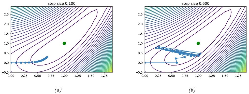
Figure 8.11: Steepest descent on a simple convex function, starting from (0, 0), for 20 steps, using a fixed step size. The global minimum is at (1, 1). (a) ↽ = 0.1. (b) ↽ = 0.6. Generated by steepestDescentDemo.ipynb.

More generally, setting ◁ < 2/L, where L is the Lipschitz constant of the gradient (Section 8.1.4), ensures convergence. Since this constant is generally unknown, we usually need to adapt the step size, as we discuss below.

8.2.2.2 Line search

The optimal step size can be found by finding the value that maximally decreases the objective along the chosen direction by solving the 1d minimization problem

\[\eta\_t = \operatorname\*{argmin}\_{\eta > 0} \phi\_t(\eta) = \operatorname\*{argmin}\_{\eta > 0} \mathcal{L}(\theta\_t + \eta \mathbf{d}\_t) \tag{8.21}\]

This is known as line search, since we are searching along the line defined by dt.

If the loss is convex, this subproblem is also convex, because ↼t(◁) = L(ω^t + ◁dt) is a convex function of an a”ne function of ◁, for fixed ω^t and dt. For example, consider the quadratic loss

\[\mathcal{L}(\boldsymbol{\theta}) = \frac{1}{2} \boldsymbol{\theta}^{\mathsf{T}} \mathbf{A} \boldsymbol{\theta} + \boldsymbol{b}^{\mathsf{T}} \boldsymbol{\theta} + c \tag{8.22}\]

Computing the derivative of ↼ gives

\[\frac{d\phi(\eta)}{d\eta} = \frac{d}{d\eta} \left[ \frac{1}{2} (\boldsymbol{\theta} + \eta \boldsymbol{d})^{\mathsf{T}} \mathbf{A} (\boldsymbol{\theta} + \eta \boldsymbol{d}) + \boldsymbol{b}^{\mathsf{T}} (\boldsymbol{\theta} + \eta \boldsymbol{d}) + c \right] \tag{8.23}\]

\[\mathbf{b} = \mathbf{d}^{\mathsf{T}} \mathbf{A} (\theta + \eta \mathbf{d}) + \mathbf{d}^{\mathsf{T}} \mathbf{b} \tag{8.24}\]

\[=\mathbf{d}^{\mathsf{T}}(\mathbf{A}\theta+\mathsf{b})+\eta\mathbf{d}^{\mathsf{T}}\mathbf{A}\mathbf{d}\tag{8.25}\]

Solving for ^d◁(φ) dφ = 0 gives

\[\eta = -\frac{d^{\mathbb{T}}(\mathbf{A}\theta + \mathbf{b})}{d^{\mathbb{T}}\mathbf{A}d} \tag{8.26}\]

Using the optimal step size is known as exact line search. However, it is not usually necessary to be so precise. There are several methods, such as the Armijo backtracking method, that try to ensure su”cient reduction in the objective function without spending too much time trying to solve Equation (8.21). In particular, we can start with the current stepsize (or some maximum value), and then reduce it by a factor 0 <c< 1 at each step until we satisfy the following condition, known as the Armijo-Goldstein test:

\[ \mathcal{L}(\boldsymbol{\theta}\_{t} + \eta \mathbf{d}\_{t}) \le \mathcal{L}(\boldsymbol{\theta}\_{t}) + c\eta \mathbf{d}\_{t}^{\mathsf{T}} \nabla \mathcal{L}(\boldsymbol{\theta}\_{t}) \tag{8.27} \]

where ^{c →} [0, 1] is a constant, typically ^c = 10→4. In practice, the initialization of the line-search and how to backtrack can significantly a!ect performance. See [NW06, Sec 3.1] for details.

8.2.3 Convergence rates

We want to find optimization algorithms that converge quickly to a (local) optimum. For certain convex problems, with a gradient with bounded Lipschitz constant, one can show that gradient descent converges at a linear rate. This means that there exists a number 0 <µ< 1 such that

\[|\mathcal{L}(\boldsymbol{\theta}\_{t+1}) - \mathcal{L}(\boldsymbol{\theta}\_{\*})| \le \mu |\mathcal{L}(\boldsymbol{\theta}\_{t}) - \mathcal{L}(\boldsymbol{\theta}\_{\*})|\tag{8.28}\]

Here µ is called the rate of convergence.

For some simple problems, we can derive the convergence rate explicitly, For example, consider a quadratic objective ^L(ω) = ^{1 2 ωT}A^ω + ^bTω + ^c with A ^∃ 0. Suppose we use steepest descent with exact line search. One can show (see e.g., [Ber15]) that the convergence rate is given by

\[ \mu = \left(\frac{\lambda\_{\text{max}} - \lambda\_{\text{min}}}{\lambda\_{\text{max}} + \lambda\_{\text{min}}}\right)^2 \tag{8.29} \]

where φmax is the largest eigenvalue of A and φmin is the smallest eigenvalue. We can rewrite this as µ = . ^κ→^{1 κ}+1 /², where ^{2 =} ↼max ↼min is the condition number of A. Intuitively, the condition number measures how “skewed” the space is, in the sense of being far from a symmetrical “bowl”. (See Section 7.1.4.4 for more information on condition numbers.)

Figure 8.12 illustrates the e!ect of the condition number on the convergence rate. On the left we show an example where A = [20, 5; 5, 2], b = [↑14; ↑6] and c = 10, so 2(A) = 30.234. On the right we show an example where A = [20, 5; 5, 16], b = [↑14; ↑6] and c = 10, so 2(A)=1.8541. We see that steepest descent converges much more quickly for the problem with the smaller condition number.

In the more general case of non-quadratic functions, the objective will often be locally quadratic around a local optimum. Hence the convergence rate depends on the condition number of the Hessian, 2(H), at that point. We can often improve the convergence speed by optimizing a surrogate objective (or model) at each step which has a Hessian that is close to the Hessian of the objective function as we discuss in Section 8.3.

Although line search works well, we see from Figure 8.12 that the path of steepest descent with an exact line-search exhibits a characteristic zig-zag behavior, which is ine”cient. This problem can be overcome using a method called conjugate gradient descent (see e.g., [She94]).

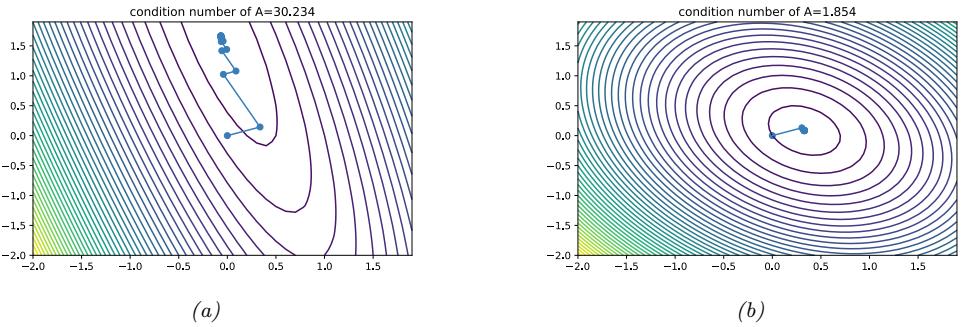
Figure 8.12: Illustration of the e!ect of condition number ⇁ on the convergence speed of steepest descent with exact line searches. (a) Large ⇁. (b) Small ⇁. Generated by lineSearchConditionNum.ipynb.

8.2.4 Momentum methods

Gradient descent can move very slowly along flat regions of the loss landscape, as we illustrated in Figure 8.11. We discuss some solutions to this below.

8.2.4.1 Momentum

One simple heuristic, known as the heavy ball or momentum method [Ber99], is to move faster along directions that were previously good, and to slow down along directions where the gradient has suddenly changed, just like a ball rolling downhill. This can be implemented as follows:

\[m\_t = \beta m\_{t-1} + g\_{t-1} \tag{8.30}\]

\[ \theta\_t = \theta\_{t-1} - \eta\_t m\_t \tag{8.31} \]

where m^t is the momentum (mass times velocity) and 0 < 1 < 1. A typical value of 1 is 0.9. For 1 = 0, the method reduces to gradient descent.

We see that m^t is like an exponentially weighted moving average of the past gradients (see Section 4.4.2.2):

\[\mathbf{m}\_{t} = \beta \mathbf{m}\_{t-1} + \mathbf{g}\_{t-1} = \beta^2 \mathbf{m}\_{t-2} + \beta \mathbf{g}\_{t-2} + \mathbf{g}\_{t-1} = \dots = \sum\_{\tau=0}^{t-1} \beta^\tau \mathbf{g}\_{t-\tau-1} \tag{8.32}\]

If all the past gradients are a constant, say g, this simplifies to

\[m\_t = \mathbf{g} \sum\_{\tau=0}^{t-1} \beta^{\tau} \tag{8.33}\]

The scaling factor is a geometric series, whose infinite sum is given by

\[1 + \beta + \beta^2 + \dots = \sum\_{i=0}^{\infty} \beta^i = \frac{1}{1 - \beta} \tag{8.34}\]

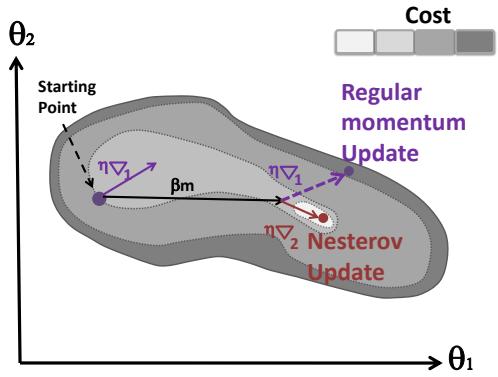
Figure 8.13: Illustration of the Nesterov update. Adapted from Figure 11.6 of [Gér19].

Thus in the limit, we multiply the gradient by 1/(1 ↑ 1). For example, if 1 = 0.9, we scale the gradient up by 10.

Since we update the parameters using the gradient average m^t→1, rather than just the most recent gradient, g^t→¹, we see that past gradients can exhibit some influence on the present. Furthermore, when momentum is combined with SGD, discussed in Section 8.4, we will see that it can simulate the e!ects of a larger minibatch, without the computational cost.

8.2.4.2 Nesterov momentum

One problem with the standard momentum method is that it may not slow down enough at the bottom of a valley, causing oscillation. The Nesterov accelerated gradient method of [Nes04] instead modifies the gradient descent to include an extrapolation step, as follows:

\[ \ddot{\theta}\_{t+1} = \theta\_t + \beta(\theta\_t - \theta\_{t-1}) \tag{8.35} \]

\[ \theta\_{t+1} = \ddot{\theta}\_{t+1} - \eta\_t \nabla \mathcal{L}(\ddot{\theta}\_{t+1}) \tag{8.36} \]

This is essentially a form of one-step “look ahead”, that can reduce the amount of oscillation, as illustrated in Figure 8.13.

Nesterov accelerated gradient can also be rewritten in the same format as standard momentum. In this case, the momentum term is updated using the gradient at the predicted new location,

\[ \delta \mathbf{m}\_{t+1} = \beta \mathbf{m}\_t - \eta\_t \nabla \mathcal{L}(\theta\_t + \beta \mathbf{m}\_t) \tag{8.37} \]

\[ \theta\_{t+1} = \theta\_t + m\_{t+1} \tag{8.38} \]

This explains why the Nesterov accelerated gradient method is sometimes called Nesterov momentum. It also shows how this method can be faster than standard momentum: the momentum vector is already roughly pointing in the right direction, so measuring the gradient at the new location, ω^t + 1mt, rather than the current location, ωt, can be more accurate.

The Nesterov accelerated gradient method is provably faster than steepest descent for convex functions when 1 and ◁^t are chosen appropriately. It is called “accelerated” because of this improved

convergence rate, which is optimal for gradient-based methods using only first-order information when the objective function is convex and has Lipschitz-continuous gradients. In practice, however, using Nesterov momentum can be slower than steepest descent, and can even unstable if 1 or ◁^t are misspecified.

8.3 Second-order methods

Optimization algorithms that only use the gradient are called first-order methods. They have the advantage that the gradient is cheap to compute and to store, but they do not model the curvature of the space, and hence they can be slow to converge, as we have seen in Figure 8.12. Second-order optimization methods incorporate curvature in various ways (e.g., via the Hessian), which may yield faster convergence. We discuss some of these methods below.

8.3.1 Newton’s method

The classic second-order method is Newton’s method. This consists of updates of the form

\[\boldsymbol{\theta}\_{t+1} = \boldsymbol{\theta}\_t - \eta\_t \mathbf{H}\_t^{-1} \mathbf{g}\_t \tag{8.39}\]

where

\[\mathbf{H}\_t \triangleq \nabla^2 \mathcal{L}(\boldsymbol{\theta})|\_{\boldsymbol{\theta}\_t} = \nabla^2 \mathcal{L}(\boldsymbol{\theta}\_t) = \mathbf{H}(\boldsymbol{\theta}\_t) \tag{8.40}\]

is assumed to be positive-definite to ensure the update is well-defined. The pseudo-code for Newton’s method is given in Algorithm 8.1. The intuition for why this is faster than gradient descent is that the matrix inverse H→¹ “undoes” any skew in the local curvature, converting a topology like Figure 8.12a to one like Figure 8.12b.

Algorithm 8.1: Newton’s method for minimizing a function

Initialize ω⁰ for t = 0, 1, 2,… until convergence do Evaluate g^t = ̸L(ωt) Evaluate ^{Ht =} ̸²L(ωt) Solve Htd^t = ↑g^t for d^t Use line search to find stepsize ◁^t along d^t ωt+1 = ω^t + ◁td^t

This algorithm can be derived as follows. Consider making a second-order Taylor series approximation of L(ω) around ωt:

\[\mathcal{L}\_{\text{quad}}(\boldsymbol{\theta}) = \mathcal{L}(\boldsymbol{\theta}\_{t}) + \boldsymbol{g}\_{t}^{\mathrm{T}}(\boldsymbol{\theta} - \boldsymbol{\theta}\_{t}) + \frac{1}{2}(\boldsymbol{\theta} - \boldsymbol{\theta}\_{t})^{\mathrm{T}}\mathbf{H}\_{t}(\boldsymbol{\theta} - \boldsymbol{\theta}\_{t})\tag{8.41}\]

The minimum of Lquad is at

\[ \theta = \theta\_t - \mathbf{H}\_t^{-1} g\_t \tag{8.42} \]

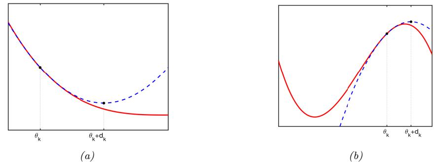
Figure 8.14: Illustration of Newton’s method for minimizing a 1d function. (a) The solid curve is the function L(x). The dotted line Lquad(ε) is its second order approximation at εt. The Newton step d^t is what must be added to ε^t to get to the minimum of Lquad(ε). Adapted from Figure 13.4 of [Van06]. Generated by newtonsMethodMinQuad.ipynb. (b) Illustration of Newton’s method applied to a nonconvex function. We fit a quadratic function around the current point ε^t and move to its stationary point, εt+1 = ε^t + dt. Unfortunately, this takes us near a local maximum of f, not minimum. This means we need to be careful about the extent of our quadratic approximation. Adapted from Figure 13.11 of [Van06]. Generated by newtonsMethodNonConvex.ipynb.

So if the quadratic approximation is a good one, we should pick ^{dt = ↑}H→^{1 t} g^t as our descent direction. See Figure 8.14(a) for an illustration. Note that, in a “pure” Newton method, we use ◁^t = 1 as our stepsize. However, we can also use linesearch to find the best stepsize; this tends to be more robust as using ◁^t = 1 may not always converge globally.

If we apply this method to linear regression, we get to the optimum in one step, since (as we show in Section 11.2.2.1) we have ^{H = XTX} and ^{g = XT}X^{w ↑ XT}y, so the Newton update becomes

\[w\_1 = w\_0 - \mathbf{H}^{-1} \mathbf{g} = w\_0 - (\mathbf{X}^\mathsf{T} \mathbf{X})^{-1} (\mathbf{X}^\mathsf{T} \mathbf{X} w\_0 - \mathbf{X}^\mathsf{T} \mathbf{y}) = w\_0 - w\_0 + (\mathbf{X}^\mathsf{T} \mathbf{X})^{-1} \mathbf{X}^\mathsf{T} \mathbf{y} \tag{8.43}\]

which is the OLS estimate. However, when we apply this method to logistic regression, it may take multiple iterations to converge to the global optimum, as we discuss in Section 10.2.6.

8.3.2 BFGS and other quasi-Newton methods

Quasi-Newton methods, sometimes called variable metric methods, iteratively build up an approximation to the Hessian using information gleaned from the gradient vector at each step. The most common method is called BFGS (named after its simultaneous inventors, Broyden, Fletcher, Goldfarb and Shanno), which updates the approximation to the Hessian B^t ↖ H^t as follows:

\[\mathbf{B}\_{t+1} = \mathbf{B}\_t + \frac{y\_t y\_t^\top}{y\_t^\top s\_t} - \frac{(\mathbf{B}\_t s\_t)(\mathbf{B}\_t s\_t)^\top}{s\_t^\top \mathbf{B}\_t s\_t} \tag{8.44}\]

\[s\_t = \theta\_t - \theta\_{t-1} \tag{8.45}\]

\[y\_t = g\_t - g\_{t-1} \tag{8.46}\]

This is a rank-two update to the matrix. If B⁰ is positive-definite, and the step size ◁ is chosen via line search satisfying both the Armijo condition in Equation (8.27) and the following curvature

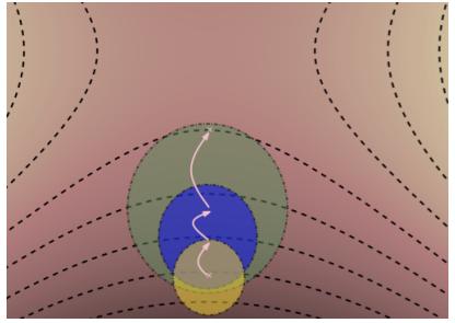
Figure 8.15: Illustration of the trust region approach. The dashed lines represents contours of the original nonconvex objective. The circles represent successive quadratic approximations. From Figure 4.2 of [Pas14]. Used with kind permission of Razvan Pascanu.

condition

\[\nabla \mathcal{L}(\boldsymbol{\theta}\_t + \eta \mathbf{d}\_t) \ge c\_2 \eta \mathbf{d}\_t^{\mathbb{T}} \nabla \mathcal{L}(\boldsymbol{\theta}\_t) \tag{8.47}\]

then Bt+1 will remain positive definite. The constant c² is chosen within (c, 1) where c is the tunable parameter in Equation (8.27). The two step size conditions are together known as the Wolfe conditions. We typically start with a diagonal approximation, B⁰ = I. Thus BFGS can be thought of as a “diagonal plus low-rank” approximation to the Hessian.

Alternatively, BFGS can iteratively update an approximation to the inverse Hessian, ^Ct ↖ ^H→^{1 t} , as follows:

\[\mathbf{C}\_{t+1} = \left(\mathbf{I} - \frac{s\_t y\_t^\top}{y\_t^\top s\_t}\right) \mathbf{C}\_t \left(\mathbf{I} - \frac{y\_t s\_t^\top}{y\_t^\top s\_t}\right) + \frac{s\_t s\_t^\top}{y\_t^\top s\_t} \tag{8.48}\]

Since storing the Hessian approximation still takes O(D²) space, for very large problems, one can use limited memory BFGS, or L-BFGS, where we control the rank of the approximation by only using the M most recent (st, yt) pairs while ignoring older information. Rather than storing B^t explicitly, we just store these vectors in memory, and then approximate H→^{1 t} g^t by performing a sequence of inner products with the stored s^t and y^t vectors. The storage requirements are therefore O(MD). Typically choosing M to be between 5–20 su”ces for good performance [NW06, p177].

Note that sklearn uses LBFGS as its default solver for logistic regression.1

8.3.3 Trust region methods

If the objective function is nonconvex, then the Hessian H^t may not be positive definite, so d^t = ^↑H→^{1 t} g^t may not be a descent direction. This is illustrated in 1d in Figure 8.14(b), which shows that Newton’s method can end up in a local maximum rather than a local minimum.

In general, any time the quadratic approximation made by Newton’s method becomes invalid, we are in trouble. However, there is usually a local region around the current iterate where we can safely

^1. See https://scikit-learn.org/stable/modules/generated/sklearn.linear\_model.LogisticRegression.html.

approximate the objective by a quadratic. Let us call this region Rt, and let us call M(⇁) the model (or approximation) to the objective, where ⇁ = ω ↑ ωt. Then at each step we can solve

\[\delta^\* = \operatorname\*{argmin}\_{\delta \in \mathcal{R}\_t} M\_t(\delta) \tag{8.49}\]

This is called trust-region optimization. (This can be seen as the “opposite” of line search, in the sense that we pick a distance we want to travel, determined by Rt, and then solve for the optimal direction, rather than picking the direction and then solving for the optimal distance.)

We usually assume that Mt(⇁) is a quadratic approximation:

\[M\_t(\boldsymbol{\delta}) = \mathcal{L}(\boldsymbol{\theta}\_t) + \boldsymbol{g}\_t^\mathsf{T}\boldsymbol{\delta} + \frac{1}{2}\boldsymbol{\delta}^\mathsf{T}\mathbf{H}\_t\boldsymbol{\delta} \tag{8.50}\]

where ^{gt =} ̸ωL(ω)|^ωt is the gradient, and ^{Ht =} ̸^{2 ω}L(ω)|^ωt is the Hessian. Furthermore, it is common to assume that R^t is a ball of radius r, i.e., R^t = {⇁ : ||⇁||² ↘ r}. Using this, we can convert the constrained problem into an unconstrained one as follows:

\[\boldsymbol{\delta}^\* = \underset{\boldsymbol{\delta}}{\operatorname{argmin}} \, M(\boldsymbol{\delta}) + \lambda ||\boldsymbol{\delta}||\_2^2 = \underset{\boldsymbol{\delta}}{\operatorname{argmin}} \, \mathbf{g}^\mathsf{T} \boldsymbol{\delta} + \frac{1}{2} \boldsymbol{\delta}^\mathsf{T} (\mathbf{H} + \lambda \mathbf{I}) \boldsymbol{\delta} \tag{8.51}\]

for some Lagrange multiplier φ > 0 which depends on the radius r (see Section 8.5.1 for a discussion of Lagrange multipliers). We can solve this using

\[\delta = -(\mathbf{H} + \lambda \mathbf{I})^{-1} \mathbf{g} \tag{8.52}\]

This is called Tikhonov damping or Tikhonov regularization. See Figure 8.15 for an illustration.

Note that adding a su”ciently large φI to H ensures the resulting matrix is always positive definite. As φ ↔︎ 0, this trust method reduces to Newton’s method, but for φ large enough, it will make all the negative eigenvalues positive (and all the 0 eigenvalues become equal to φ).

8.4 Stochastic gradient descent

In this section, we consider stochastic optimization, where the goal is to minimize the average value of a function:

\[\mathcal{L}(\boldsymbol{\theta}) = \mathbb{E}\_{\mathbf{q}(\mathbf{z})} \left[ \mathcal{L}(\boldsymbol{\theta}, \mathbf{z}) \right] \tag{8.53}\]

where z is a random input to the objective. This could be a “noise” term, coming from the environment, or it could be a training example drawn randomly from the training set, as we explain below.

At each iteration, we assume we observe Lt(ω) = L(ω, zt), where z^t ⇒ q. We also assume a way to compute an unbiased estimate of the gradient of L. If the distribution q(z) is independent of the parameters we are optimizing, we can use g^t = ̸ωLt(ωt). In this case, the resulting algorithm can be written as follows:

\[ \theta\_{t+1} = \theta\_t - \eta\_t \nabla\_{\theta} \mathcal{L}(\theta\_t, \mathbf{z}\_t) = \theta\_t - \eta\_t \mathbf{g}\_t \tag{8.54} \]

This method is known as stochastic gradient descent or SGD. As long as the gradient estimate is unbiased, then this method will converge to a stationary point, providing we decay the step size ◁^t at a certain rate, as we discuss in Section 8.4.3.

8.4.1 Application to finite sum problems

SGD is very widely used in machine learning. To see why, recall from Section 4.3 that many model fitting procedures are based on empirical risk minimization, which involve minimizing the following loss:

\[\mathcal{L}(\boldsymbol{\theta}\_{t}) = \frac{1}{N} \sum\_{n=1}^{N} \ell(y\_n, f(\boldsymbol{x}\_n; \boldsymbol{\theta}\_t)) = \frac{1}{N} \sum\_{n=1}^{N} \mathcal{L}\_n(\boldsymbol{\theta}\_t) \tag{8.55}\]

This is called a finite sum problem. The gradient of this objective has the form

\[\mathbf{g}\_t = \frac{1}{N} \sum\_{n=1}^{N} \nabla\_{\theta} \mathcal{L}\_n(\theta\_t) = \frac{1}{N} \sum\_{n=1}^{N} \nabla\_{\theta} \ell(y\_n, f(x\_n; \theta\_t)) \tag{8.56}\]

This requires summing over all N training examples, and thus can be slow if N is large. Fortunately we can approximate this by sampling a minibatch of B A N samples to get

\[\mathfrak{g}\_t \approx \frac{1}{|\mathcal{B}\_t|} \sum\_{n \in \mathcal{B}\_t} \nabla\_{\theta} \mathcal{L}\_n(\theta\_t) = \frac{1}{|\mathcal{B}\_t|} \sum\_{n \in \mathcal{B}\_t} \nabla\_{\theta} \ell(y\_n, f(x\_n; \theta\_t)) \tag{8.57}\]

where B^t is a set of randomly chosen examples to use at iteration t. 2 This is an unbiased approximation to the empirical average in Equation (8.56). Hence we can safely use this with SGD.

Although the theoretical rate of convergence of SGD is slower than batch GD (in particular, SGD has a sublinear convergence rate), in practice SGD is often faster, since the per-step time is much lower [BB08; BB11]. To see why SGD can make faster progress than full batch GD, suppose we have a dataset consisting of a single example duplicated K times. Batch training will be (at least) K times slower than SGD, since it will waste time computing the gradient for the repeated examples. Even if there are no duplicates, batch training can be wasteful, since early on in training the parameters are not well estimated, so it is not worth carefully evaluating the gradient.

8.4.2 Example: SGD for fitting linear regression

In this section, we show how to use SGD to fit a linear regression model. Recall from Section 4.2.7 that the objective has the form

\[\mathcal{L}(\boldsymbol{\theta}) = \frac{1}{2N} \sum\_{n=1}^{N} (\mathbf{z}\_n^\mathsf{T} \boldsymbol{\theta} - y\_n)^2 = \frac{1}{2N} ||\mathbf{X} \boldsymbol{\theta} - \boldsymbol{y}||\_2^2 \tag{8.58}\]

The gradient is

\[\mathbf{g}\_t = \frac{1}{N} \sum\_{n=1}^{N} (\boldsymbol{\theta}\_t^\top \boldsymbol{x}\_n - y\_n) \mathbf{x}\_n \tag{8.59}\]

^2. In practice we usually sample B^t without replacement. However, once we reach the end of the dataset (i.e., after a single training epoch), we can perform a random shu”ing of the examples, to ensure that each minibatch on the next epoch is di!erent from the last. This version of SGD is analyzed in [HS19].

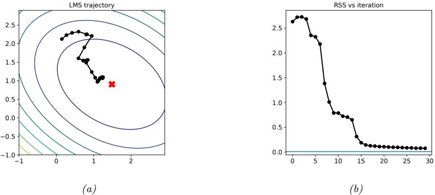
Figure 8.16: Illustration of the LMS algorithm. Left: we start from ω = (↑0.5, 2) and slowly converging to the least squares solution of ωˆ = (1.45, 0.93) (red cross). Right: plot of objective function over time. Note that it does not decrease monotonically. Generated by lms\_demo.ipynb.

Now consider using SGD with a minibatch size of B = 1. The update becomes

\[\boldsymbol{\theta}\_{t+1} = \boldsymbol{\theta}\_t - \eta\_t (\boldsymbol{\theta}\_t^\top \boldsymbol{x}\_n - y\_n) \mathbf{z}\_n \tag{8.60}\]

where n = n(t) is the index of the example chosen at iteration t. The overall algorithm is called the least mean squares (LMS) algorithm, and is also known as the delta rule, or the Widrow-Ho” rule.

Figure 8.16 shows the results of applying this algorithm to the data shown in Figure 11.2. We start at ^ω = (↑0.5, 2) and converge (in the sense that ||ω^{t ↑ ωt}→¹||^{2 2} drops below a threshold of 10→2) in about 26 iterations. Note that SGD (and hence LMS) may require multiple passes through the data to find the optimum.

8.4.3 Choosing the step size (learning rate)

When using SGD, we need to be careful in how we choose the learning rate in order to achieve convergence. For example, in Figure 8.17 we plot the loss vs the learning rate when we apply SGD to a deep neural network classifier (see Chapter 13 for details). We see a U-shaped curve, where an overly small learning rate results in underfitting, and overly large learning rate results in instability of the model (c.f., Figure 8.11(b)); in both cases, we fail to converge to a local optimum.

One heuristic for choosing a good learning rate, proposed in [Smi18], is to start with a small learning rate and gradually increase it, evaluating performance using a small number of minibatches. We then make a plot like the one in Figure 8.17, and pick the learning rate with the lowest loss. (In practice, it is better to pick a rate that is slightly smaller than (i.e., to the left of) the one with the lowest loss, to ensure stability.)

Rather than choosing a single constant learning rate, we can use a learning rate schedule, in which we adjust the step size over time. Theoretically, a su”cient condition for SGD to achieve

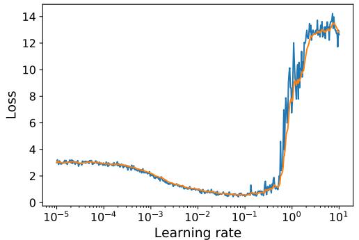
Figure 8.17: Loss vs learning rate (horizontal axis). Training loss vs learning rate for a small MLP fit to FashionMNIST using vanilla SGD. (Raw loss in blue, EWMA smoothed version in orange). Generated by lrschedule\_tf.ipynb.

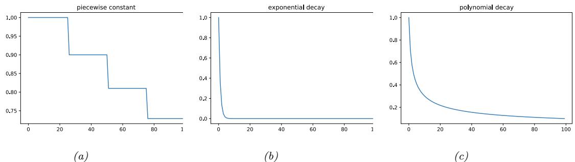
Figure 8.18: Illustration of some common learning rate schedules. (a) Piecewise constant. (b) Exponential decay. (c) Polynomial decay. Generated by learning\_rate\_plot.ipynb.

convergence is if the learning rate schedule satisfies the Robbins-Monro conditions:

\[ \eta\_t \to 0, \ \frac{\sum\_{t=1}^{\infty} \eta\_t^2}{\sum\_{t=1}^{\infty} \eta\_t} \to 0 \tag{8.61} \]

Some common examples of learning rate schedules are listed below:

• ◁^t = ◁ⁱ if tⁱ ↘ t ↘ ti+1 piecewise constant (8.62)
• ◁^t = ◁0e→↼^t exponential decay (8.63)

\[ \eta\_t = \eta\_0 (\beta t + 1)^{-\alpha} \text{ polynomial decay} \tag{8.64} \]

In the piecewise constant schedule, tⁱ are a set of time points at which we adjust the learning rate to a specified value. For example, we may set ◁ⁱ = ◁0⇁ⁱ , which reduces the initial learning rate by a factor of ⇁ for each threshold (or milestone) that we pass. Figure 8.18a illustrates this for ◁⁰ = 1

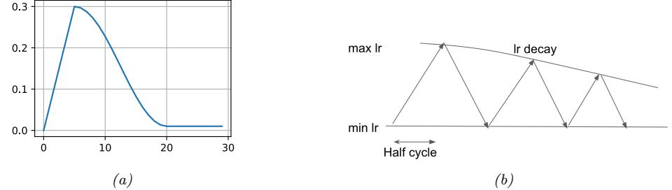
Figure 8.19: (a) Linear warm-up followed by cosine cool-down. (b) Cyclical learning rate schedule.

and ⇁ = 0.9. This is called step decay. Sometimes the threshold times are computed adaptively, by estimating when the train or validation loss has plateaued; this is called reduce-on-plateau. Exponential decay is typically too fast, as illustrated in Figure 8.18b. A common choice is polynomial decay, with ϱ = 0.5 and 1 = 1, as illustrated in Figure 8.18c; this corresponds to a square-root schedule, ◁^t = ◁⁰ ⇐ 1 ^t+1 .

In the deep learning community, another common schedule is to quickly increase the learning rate and then gradually decrease it again, as shown in Figure 8.19a. This is called learning rate warmup, or the one-cycle learning rate schedule [Smi18]. The motivation for this is the following: initially the parameters may be in a part of the loss landscape that is poorly conditioned, so a large step size will “bounce around” too much (c.f., Figure 8.11(b)) and fail to make progress downhill. However, with a slow learning rate, the algorithm can discover flatter regions of space, where a larger step size can be used. Once there, fast progress can be made. However, to ensure convergence to a point, we must reduce the learning rate to 0. See [Got+19; Gil+21] for more details.

It is also possible to increase and decrease the learning rate multiple times, in a cyclical fashion. This is called a cyclical learning rate [Smi18], and was popularized by the <fast.ai> course. See Figure 8.19b for an illustration using triangular shapes. The motivation behind this approach is to escape local minima. The minimum and maximum learning rates can be found based on the initial “dry run” described above, and the half-cycle can be chosen based on how many restarts you want to do with your training budget. A related approach, known as stochastic gradient descent with warm restarts, was proposed in [LH17]; they proposed storing all the checkpoints visited after each cool down, and using all of them as members of a model ensemble. (See Section 18.2 for a discussion of ensemble learning.)

An alternative to using heuristics for estimating the learning rate is to use line search (Section 8.2.2.2). This is tricky when using SGD, because the noisy gradients make the computation of the Armijo condition di”cult [CS20]. However, [Vas+19] show that it can be made to work if the variance of the gradient noise goes to zero over time. This can happen if the model is su”ciently flexible that it can perfectly interpolate the training set.

8.4.4 Iterate averaging

The parameter estimates produced by SGD can be very unstable over time. To reduce the variance of the estimate, we can compute the average using

\[\overline{\theta}\_{t} = \frac{1}{t} \sum\_{i=1}^{t} \theta\_{i} = \frac{1}{t} \theta\_{t} + \frac{t-1}{t} \overline{\theta}\_{t-1} \tag{8.65}\]

where ω^t are the usual SGD iterates. This is called iterate averaging or Polyak-Ruppert averaging [Rup88].

In [PJ92], they prove that the estimate ω^t achieves the best possible asymptotic convergence rate among SGD algorithms, matching that of variants using second-order information, such as Hessians.

This averaging can also have statistical benefits. For example, in [NR18], they prove that, in the case of linear regression, this method is equivalent to ω² regularization (i.e., ridge regression).

Rather than an exponential moving average of SGD iterates, Stochastic Weight Averaging (SWA) [Izm+18] uses an equal average in conjunction with a modified learning rate schedule. In contrast to standard Polyak-Ruppert averaging, which was motivated for faster convergence rates, SWA exploits the flatness in objectives used to train deep neural networks, to find solutions which provide better generalization.

8.4.5 Variance reduction *

In this section, we discuss various ways to reduce the variance in SGD. In some cases, this can improve the theoretical convergence rate from sublinear to linear (i.e., the same as full-batch gradient descent) [SLRB17; JZ13; DBLJ14]. These methods reduce the variance of the gradients, rather than the parameters themselves and are designed to work for finite sum problems.

8.4.5.1 SVRG

The basic idea of stochastic variance reduced gradient (SVRG) [JZ13] is to use a control variate, in which we estimate a baseline value of the gradient based on the full batch, which we then use to compare the stochastic gradients to.

More precisely, ever so often (e.g., once per epoch), we compute the full gradient at a “snapshot” of the model parameters ^ω˜; the corresponding “exact” gradient is therefore ̸L(ω˜). At step ^t, we compute the usual stochastic gradient at the current parameters, ̸Lt(ωt), but also at the snapshot parameters, ̸Lt(ω˜), which we use as a baseline. We can then use the following improved gradient estimate

\[\mathbf{g}\_t = \nabla \mathcal{L}\_t(\boldsymbol{\theta}\_t) - \nabla \mathcal{L}\_t(\boldsymbol{\tilde{\theta}}) + \nabla \mathcal{L}(\boldsymbol{\tilde{\theta}}) \tag{8.66}\]

to compute ωt+1. This is unbiased because E ̸Lt(ω˜) ⁼ ̸L(ω˜). Furthermore, the update only involves two gradient computations, since we can compute ̸L(ω˜) once per epoch. At the end of the epoch, we update the snapshot parameters, ω˜, based on the most recent value of ωt, or a running average of the iterates, and update the expected baseline. (We can compute snapshots less often, but then the baseline will not be correlated with the objective and can hurt performance, as shown in [DB18].)

Iterations of SVRG are computationally faster than those of full-batch GD, but SVRG can still match the theoretical convergence rate of GD.

8.4.5.2 SAGA

In this section, we describe the stochastic averaged gradient accelerated (SAGA) algorithm of [DBLJ14]. Unlike SVRG, it only requires one full batch gradient computation, at the start of the algorithm. However, it “pays” for this saving in time by using more memory. In particular, it must store N gradient vectors. This enables the method to maintain an approximation of the global gradient by removing the old local gradient from the overall sum and replacing it with the new local gradient. This is called an aggregated gradient method.

More precisely, we first initialize by computing glocal ⁿ = ̸Ln(ω0) for all n, and the average, gavg = ¹ N $^{N n}=1 glocal ⁿ . Then, at iteration t, we use the gradient estimate

\[\mathbf{g}\_t = \nabla \mathcal{L}\_n(\boldsymbol{\theta}\_t) - \mathbf{g}\_n^{\text{local}} + \mathbf{g}^{\text{avg}} \tag{8.67}\]

where ^{n ⇒} Unif{1,…,N} is the example index sampled at iteration ^t. We then update ^glocal ⁿ = ̸Ln(ωt) and ^gavg by replacing the old ^glocal ⁿ by its new value.

This has an advantage over SVRG since it only has to do one full batch sweep at the start. (In fact, the initial sweep is not necessary, since we can compute gavg “lazily”, by only incorporating gradients we have seen so far.) The downside is the large extra memory cost. However, if the features (and hence gradients) are sparse, the memory cost can be reasonable. Indeed, the SAGA algorithm is recommended for use in the sklearn logistic regression code when N is large and x is sparse.3

8.4.5.3 Application to deep learning

Variance reduction methods are widely used for fitting ML models with convex objectives, such as linear models. However, there are various di”culties associated with using SVRG with conventional deep learning training practices. For example, the use of batch normalization (Section 14.2.4.1), data augmentation (Section 19.1) and dropout (Section 13.5.4) all break the assumptions of the method, since the loss will di!er randomly in ways that depend not just on the parameters and the data index n. For more details, see e.g., [DB18; Arn+19].

8.4.6 Preconditioned SGD

In this section, we consider preconditioned SGD, which involves the following update:

\[ \boldsymbol{\theta}\_{t+1} = \boldsymbol{\theta}\_t - \eta\_t \mathbf{M}\_t^{-1} \boldsymbol{g}\_t,\tag{8.68} \]

where M^t is a preconditioning matrix, or simply the preconditioner, typically chosen to be positive-definite. Unfortunately the noise in the gradient estimates make it di”cult to reliably estimate the Hessian, which makes it di”cult to use the methods from Section 8.3. In addition, it is expensive to solve for the update direction with a full preconditioning matrix. Therefore most practitioners use a diagonal preconditioner Mt. Such preconditioners do not necessarily use second-order information, but often result in speedups compared to vanilla SGD. See also [Roo+21]

^3. See https://scikit-learn.org/stable/modules/linear\_model.html#logistic-regression.

for a probabilitic interpretation of these heuristics, and sgd\_comparison.ipynb for an empirical comparison on some simple datasets.

8.4.6.1 AdaGrad

The AdaGrad (short for “adaptive gradient”) method of [DHS11] was originally designed for optimizing convex objectives where many elements of the gradient vector are zero; these might correspond to features that are rarely present in the input, such as rare words. The update has the following form

\[ \theta\_{t+1,d} = \theta\_{t,d} - \eta\_t \frac{1}{\sqrt{s\_{t,d} + \epsilon}} g\_{t,d} \tag{8.69} \]

where d =1: D indexes the dimensions of the parameter vector, and

\[s\_{t,d} = \sum\_{i=1}^{t} g\_{i,d}^2 \tag{8.70}\]

is the sum of the squared gradients and ▷ > 0 is a small term to avoid dividing by zero. Equivalently we can write the update in vector form as follows:

\[ \Delta\theta\_t = -\eta\_t \frac{1}{\sqrt{\mathbf{s}\_t + \epsilon}} \mathbf{g}\_t \tag{8.71} \]

where the square root and division is performed elementwise. Viewed as preconditioned SGD, this is equivalent to taking M^t = diag(s^t + ,)¹/². This is an example of an adaptive learning rate; the overall stepsize ◁^t still needs to be chosen, but the results are less sensitive to it compared to vanilla GD. In particular, we usually fix ◁^t = ◁0.

8.4.6.2 RMSProp and AdaDelta

A defining feature of AdaGrad is that the term in the denominator gets larger over time, so the e!ective learning rate drops. While it is necessary to ensure convergence, it might hurt performance as the denominator gets large too fast.

An alternative is to use an exponentially weighted moving average (EWMA, Section 4.4.2.2) of the past squared gradients, rather than their sum:

\[s\_{t+1,d} = \beta s\_{t,d} + (1 - \beta)g\_{t,d}^2 \tag{8.72}\]

In practice we usually use 1 ⇒ 0.9, which puts more weight on recent examples. In this case,

\[\sqrt{s\_{t,d}} \approx \text{RMS}(\mathbf{g}\_{1:t,d}) = \sqrt{\frac{1}{t} \sum\_{\tau=1}^{t} g\_{\tau,d}^2} \tag{8.73}\]

where RMS stands for “root mean squared”. Hence this method, (which is based on the earlier RPROP method of [RB93]) is known as RMSProp [Hin14]. The overall update of RMSProp is

\[ \Delta\theta\_t = -\eta\_t \frac{1}{\sqrt{s\_t + \epsilon}} g\_t. \tag{8.74} \]

The AdaDelta method was independently introduced in [Zei12], and is similar to RMSprop. However, in addition to accumulating an EWMA of the gradients in sˆ, it also keeps an EWMA of the updates ⇁^t to obtain an update of the form

\[ \Delta\theta\_t = -\eta\_t \frac{\sqrt{\delta\_{t-1} + \epsilon}}{\sqrt{\mathbf{s}\_t + \epsilon}} \mathbf{g}\_t \tag{8.75} \]

where

\[ \delta \mathfrak{d}\_t = \beta \mathfrak{d}\_{t-1} + (1 - \beta)(\Delta \mathfrak{H}\_t)^2 \tag{8.76} \]

and s^t is the same as in RMSProp. This has the advantage that the “units” of the numerator and denominator cancel, so we are just elementwise-multiplying the gradient by a scalar. This eliminates the need to tune the learning rate ◁t, which means one can simply set ◁^t = 1, although popular implementations of AdaDelta still keep ◁^t as a tunable hyperparameter. However, since these adaptive learning rates need not decrease with time (unless we choose ◁^t to explicitly do so), these methods are not guaranteed to converge to a solution.

8.4.6.3 Adam

It is possible to combine RMSProp with momentum. In particular, let us compute an EWMA of the gradients (as in momentum) and squared gradients (as in RMSProp)

\[ \mathbf{m}\_t = \beta\_1 \mathbf{m}\_{t-1} + (1 - \beta\_1)\mathbf{g}\_t \tag{8.77} \]

\[\mathbf{s}\_{t} = \beta\_{2}\mathbf{s}\_{t-1} + (1 - \beta\_{2})\mathbf{g}\_{t}^{2} \tag{8.78}\]

We then perform the following update:

\[ \theta\_t = \theta\_t - \eta\_t \frac{m\_t}{\sqrt{\mathbf{s}\_t} + \epsilon} \tag{8.79} \]

The resulting method is known as Adam, which stands for “adaptive moment estimation” [KB15].

The standard values for the various constants are 1¹ = 0.9, 1² = 0.999 and ▷ = 10→⁶. (If we set 1¹ = 0 and no bias-correction, we recover RMSProp, which does not use momentum.) For the overall learning rate, it is common to use a fixed value such as ◁^t = 0.001. Again, as the adaptive learning rate may not decrease over time, convergence is not guaranteed (see Section 8.4.6.4).

If we initialize with m⁰ = s⁰ = 0, then initial estimates will be biased towards small values. The authors therefore recommend using the bias-corrected moments, which increase the values early in the optimization process. These estimates are given by

\[ \hat{m}\_t = \mathbf{m}\_t / (1 - \beta\_1^t) \tag{8.80} \]

\[\hat{\mathbf{s}}\_t = \mathbf{s}\_t / (1 - \beta\_2^t) \tag{8.81}\]

The advantage of bias-correction is shown in Figure 4.3.

8.4.6.4 Issues with adaptive learning rates

When using diagonal scaling methods, the overall learning rate is determined by ◁0M→^{1 t} , which changes with time. Hence these methods are often called adaptive learning rate methods. However, they still require setting the base learning rate ◁0.

Since the EWMA methods are typically used in the stochastic setting where the gradient estimates are noisy, their learning rate adaptation can result in non-convergence even on convex problems [RKK18]. In [Zha+22] they show experimentally that vanilla Adam can be made to converge provided the 1¹ and 1² parameters are tuned on a per-dataset basis, but it is better to find an automatic, robust method. Various solutions to this problem have been proposed, including AMSGrad [RKK18], Padam [CG18; Zho+18], and Yogi [Zah+18]. For example, the Yogi update modifies Adam by replacing

\[\mathbf{s}\_{t} = \beta\_{2}\mathbf{s}\_{t-1} + (1 - \beta\_{2})\mathbf{g}\_{t}^{2} = \mathbf{s}\_{t-1} + (1 - \beta\_{2})(\mathbf{g}\_{t}^{2} - \mathbf{s}\_{t-1})\tag{8.82}\]

with

\[\mathbf{s}\_{t} = \mathbf{s}\_{t-1} + (1 - \beta\_2)\mathbf{g}\_t^2 \odot \text{sgn}(\mathbf{g}\_t^2 - \mathbf{s}\_{t-1}) \tag{8.83}\]

More recently, [Tan+24] proposed ADOPT, which not only results in provable convergence, but also seems to work better in practice. The basic idea is to normalize (precondition) the gradient before computing the momentum update, i.e., we use m^t = 11m^t→¹ + (1 ↑ 11) ⇐ gt ^st↓1+, instead of m^t = 11m^t→¹ + (1 ↑ 11)gt. We also now update the parameters using ω^t = ω^t ↑ ◁tm^t instead of ^{ωt = ωt ↑ ◁t} ⇐m^{t s}t+, .

8.4.6.5 Non-diagonal preconditioning matrices

Although the methods we have discussed above can adapt the learning rate of each parameter, they do not solve the more fundamental problem of ill-conditioning due to correlation of the parameters, and hence do not always provide as much of a speed boost over vanilla SGD as one may hope.

One way to get faster convergence is to use the following preconditioning matrix, known as full-matrix Adagrad [DHS11]:

\[\mathbf{M}\_t = \left[ (\mathbf{G}\_t \mathbf{G}\_t^T)^{\frac{1}{2}} + \epsilon \mathbf{I}\_D \right]^{-1} \tag{8.84}\]

where

\[\mathbf{G}\_{t} = [\mathbf{g}\_{t}, \dots, \mathbf{g}\_{1}] \tag{8.85}\]

Here gⁱ = ̸ϱc(ψi) is the D-dimensional gradient vector computed at step i. Unfortunately, M^t is a D ↓ D matrix, which is expensive to store and invert.

The Shampoo algorithm [GKS18] makes a block diagonal approximation to M, one per layer of the model, and then exploits Kronecker product structure to e”ciently invert it. (It is called “shampoo” because it uses a conditioner.) Recently, [Ani+20] scaled this method up to fit very large deep models in record time.

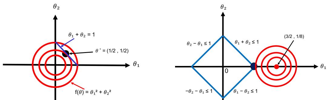
Figure 8.20: Illustration of some constrained optimization problems. Red contours are the level sets of the objective function L(ω). Optimal constrained solution is the black dot, (a) Blue line is the equality constraint h(ω)=0. (b) Blue lines denote the inequality constraints |ε1| + |ε2| ↗ 1. (Compare to Figure 11.8 (left).)

8.5 Constrained optimization

In this section, we consider the following constrained optimization problem:

\[\boldsymbol{\theta}^\* = \arg\min\_{\boldsymbol{\theta} \in \mathcal{C}} \mathcal{L}(\boldsymbol{\theta}) \tag{8.86}\]

where the feasible set, or constraint set, is

\[\mathcal{C} = \{ \boldsymbol{\theta} \in \mathbb{R}^{D} : h\_i(\boldsymbol{\theta}) = 0, i \in \mathcal{E}, \ g\_j(\boldsymbol{\theta}) \le 0, j \in \mathcal{T} \}\tag{8.87}\]

where E is the set of equality constraints, and I is the set of inequality constraints.

For example, suppose we have a quadratic objective, ^L(ω) = ^{ϖ2 1} + ϖ^{2 2}, subject to a linear equality constraint, h(ω)=1 ↑ ϖ¹ ↑ ϖ² = 0. Figure 8.20(a) plots the level sets of L, as well as the constraint surface. What we are trying to do is find the point ω^↓ that lives on the line, but which is closest to the origin. It is clear from the geometry that the optimal solution is ω = (0.5, 0.5), indicated by the solid black dot.

In the following sections, we briefly describe some of the theory and algorithms underlying constrained optimization. More details can be found in other books, such as [BV04; NW06; Ber15; Ber16].

8.5.1 Lagrange multipliers

In this section, we discuss how to solve equality contrained optimization problems. We initially assume that we have just one equality constraint, h(ω)=0.

First note that for any point on the constraint surface, ̸h(ω) will be orthogonal to the constraint surface. To see why, consider another point nearby, ω + ,, that also lies on the surface. If we make a first-order Taylor expansion around ω we have

\[h(\theta + \epsilon) \approx h(\theta) + \epsilon^{\Upsilon} \nabla h(\theta) \tag{8.88}\]

Since both ω and ω + , are on the constraint surface, we must have h(ω) = h(ω + ,) and hence ,T̸h(ω) ↖ ⁰. Since , is parallel to the constraint surface, ̸h(ω) must be perpendicular to it.

We seek a point ω^↓ on the constraint surface such that L(ω) is minimized. We just showed that it must satisfy the condition that ̸h(ω↓) is orthogonal to the constraint surface. In addition, such a point must have the property that ̸L(ω) is also orthogonal to the constraint surface, as otherwise we could decrease L(ω) by moving a short distance along the constraint surface. Since both ̸h(ω) and ̸L(ω) are orthogonal to the constraint surface at ω↓, they must be parallel (or anti-parallel) to each other. Hence there must exist a constant φ^↓ → R such that

\[ \nabla \mathcal{L}(\boldsymbol{\theta}^\*) = \lambda^\* \nabla h(\boldsymbol{\theta}^\*) \tag{8.89} \]

(We cannot just equate the gradient vectors, since they may have di!erent magnitudes.) The constant φ^↓ is called a Lagrange multiplier, and can be positive, negative, or zero. This latter case occurs when ̸L(ω↓)=0.

We can convert Equation (8.89) into an objective, known as the Lagrangian, that we should find a stationary point of the following:

\[L(\theta, \lambda) \triangleq \mathcal{L}(\theta) + \lambda h(\theta) \tag{8.90}\]

At a stationary point of the Lagrangian, we have

\[ \nabla\_{\theta,\lambda} L(\theta,\lambda) = \mathbf{0} \iff \lambda \nabla\_{\theta} h(\theta) = \nabla \mathcal{L}(\theta), \ h(\theta) = 0 \tag{8.91} \]

This is called a critical point, and satisfies the original constraint h(ω)=0 and Equation (8.89).

If we have m > 1 constraints, we can form a new constraint function by addition, as follows:

\[L(\theta, \lambda) = \mathcal{L}(\theta) + \sum\_{j=1}^{m} \lambda\_j h\_j(\theta) \tag{8.92}\]

We now have D+m equations in D+m unknowns and we can use standard unconstrained optimization methods to find a stationary point. We give some examples below.

8.5.1.1 Example: 2d Quadratic objective with one linear equality constraint

Consider minimizing ^L(ω) = ^{ϖ2 1} + ϖ^{2 2} subject to the constraint that ϖ¹ + ϖ² = 1. (This is the problem illustrated in Figure 8.20(a).) The Lagrangian is

\[L(\theta\_1, \theta\_2, \lambda) = \theta\_1^2 + \theta\_2^2 + \lambda(\theta\_1 + \theta\_2 - 1) \tag{8.93}\]

We have the following conditions for a stationary point:

\[\frac{\partial}{\partial \theta\_1} L(\theta\_1, \theta\_2, \lambda) = 2\theta\_1 + \lambda = 0 \tag{8.94}\]

\[\frac{\partial}{\partial \theta\_2} L(\theta\_1, \theta\_2, \lambda) = 2\theta\_2 + \lambda = 0 \tag{8.95}\]

\[\frac{\partial}{\partial \lambda} L(\theta\_1, \theta\_2, \lambda) = \theta\_1 + \theta\_2 - 1 = 0 \tag{8.96}\]

From Equations 8.94 and 8.95 we find 2ϖ¹ = ↑φ = 2ϖ2, so ϖ¹ = ϖ2. Also, from Equation (8.96), we find 2ϖ¹ = 1. So ω^↓ = (0.5, 0.5), as we claimed earlier. Furthermore, this is the global minimum since the objective is convex and the constraint is a”ne.

8.5.2 The KKT conditions

In this section, we generalize the concept of Lagrange multipliers to additionally handle inequality constraints.

First consider the case where we have a single inequality constraint g(ω) ↘ 0. To find the optimum, one approach would be to consider an unconstrained problem where we add the penalty as an infinite step function:

\[ \hat{\mathcal{L}}(\theta) = \mathcal{L}(\theta) + \infty \mathbb{I}\left(g(\theta) > 0\right) \tag{8.97} \]

However, this is a discontinuous function that is hard to optimize.

Instead, we create a lower bound of the form µg(ω), where µ ∋ 0. This gives us the following Lagrangian:

\[L(\theta, \mu) = \mathcal{L}(\theta) + \mu g(\theta) \tag{8.98}\]

Note that the step function can be recovered using

\[\hat{\mathcal{L}}(\boldsymbol{\theta}) = \max\_{\mu \ge 0} L(\boldsymbol{\theta}, \mu) = \begin{cases} \infty & \text{if } g(\boldsymbol{\theta}) > 0, \\ \mathcal{L}(\boldsymbol{\theta}) & \text{otherwise} \end{cases} \tag{8.99}\]

Thus our optimization problem becomes

\[\min\_{\theta} \max\_{\mu \ge 0} L(\theta, \mu) \tag{8.100}\]

Now consider the general case where we have multiple inequality constraints, g(ω) ↘ 0, and multiple equality constraints, h(ω) = 0. The generalized Lagrangian becomes

\[L(\theta, \mu, \lambda) = \mathcal{L}(\theta) + \sum\_{i} \mu\_i g\_i(\theta) + \sum\_{j} \lambda\_j h\_j(\theta) \tag{8.101}\]

(We are free to change ↑φjh^j to +φjh^j since the sign is arbitrary.) Our optimization problem becomes

\[\min\_{\theta} \max\_{\mu \ge 0, \lambda} L(\theta, \mu, \lambda) \tag{8.102}\]

When L and g are convex, then all critical points of this problem must satisfy the following criteria (under some conditions [BV04, Sec.5.2.3]):

• All constraints are satisfied (this is called feasibility):

\[g(\theta) \le 0, \ h(\theta) = 0\tag{8.103}\]

• The solution is a stationary point:

\[ \nabla \mathcal{L}(\boldsymbol{\theta}^\*) + \sum\_i \mu\_i \nabla g\_i(\boldsymbol{\theta}^\*) + \sum\_j \lambda\_j \nabla h\_j(\boldsymbol{\theta}^\*) = \mathbf{0} \tag{8.104} \]

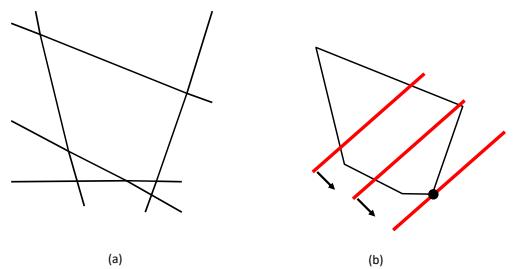
Figure 8.21: (a) A convex polytope in 2d defined by the intersection of linear constraints. (b) Depiction of the feasible set as well as the linear objective function. The red line is a level set of the objective, and the arrow indicates the direction in which it is improving. We see that the optimal solution lies at a vertex of the polytope.

• The penalty for the inequality constraint points in the right direction (this is called dual feasibility):

\[ \mu \ge 0 \tag{8.105} \]

• The Lagrange multipliers pick up any slack in the inactive constraints, i.e., either µⁱ = 0 or gi(ω↓)=0, so

\[ \mu \odot \mathfrak{g} = \mathbf{0} \tag{8.106} \]

This is called complementary slackness.

To see why the last condition holds, consider (for simplicity) the case of a single inequality constraint, g(ω) ↘ 0. Either it is active, meaning g(ω)=0, or it is inactive, meaning g(ω) < 0. In the active case, the solution lies on the constraint boundary, and g(ω)=0 becomes an equality constraint; then we have ̸L = µ̸g for some constant µ ↗= 0, because of Equation (8.89). In the inactive case, the solution is not on the constraint boundary; we still have ̸L = µ̸g, but now µ = 0.

These are called the Karush-Kuhn-Tucker (KKT) conditions. If L is a convex function, and the constraints define a convex set, the KKT conditions are su”cient for (global) optimality, as well as necessary.

8.5.3 Linear programming

Consider optimizing a linear function subject to linear constraints. When written in standard form, this can be represented as

\[\min\_{\theta} \mathbf{c}^{\mathsf{T}} \theta \qquad \text{s.t.} \quad \mathbf{A}\theta \le \mathbf{b}, \ \theta \ge 0 \tag{8.107}\]

The feasible set defines a convex polytope, which is a convex set defined as the intersection of half spaces. See Figure 8.21(a) for a 2d example. Figure 8.21(b) shows a linear cost function that

decreases as we move to the bottom right. We see that the lowest point that is in the feasible set is a vertex. In fact, it can be proved that the optimum point always occurs at a vertex of the polytope, assuming the solution is unique. If there are multiple solutions, the line will be parallel to a face. There may also be no optima inside the feasible set; in this case, the problem is said to be infeasible.

8.5.3.1 The simplex algorithm

It can be shown that the optima of an LP occur at vertices of the polytope defining the feasible set (see Figure 8.21(b) for an example). The simplex algorithm solves LPs by moving from vertex to vertex, each time seeking the edge which most improves the objective.

In the worst-case scenario, the simplex algorithm can take time exponential in D, although in practice it is usually very e”cient. There are also various polynomial-time algorithms, such as the interior point method, although these are often slower in practice.

8.5.3.2 Applications

There are many applications of linear programming in science, engineering and business. It is also useful in some machine learning problems. For example, Section 11.6.1.1 shows how to use it to solve robust linear regression. It is also useful for state estimation in graphical models (see e.g., [SGJ11]).

8.5.4 Quadratic programming

Consider minimizing a quadratic objective subject to linear equality and inequality constraints. This kind of problem is known as a quadratic program or QP, and can be written as follows:

\[\min\_{\theta} \frac{1}{2} \theta^{\mathsf{T}} \mathbf{H} \theta + \mathbf{c}^{\mathsf{T}} \theta \quad \text{s.t.} \quad \mathbf{A} \theta \le b, \ \mathsf{C} \theta = d\]

If H is positive semidefinite, then this is a convex optimization problem.

8.5.4.1 Example: 2d quadratic objective with linear inequality constraints

As a concrete example, suppose we want to minimize

\[\mathcal{L}(\boldsymbol{\theta}) = (\theta\_1 - \frac{3}{2})^2 + (\theta\_2 - \frac{1}{8})^2 = \frac{1}{2}\boldsymbol{\theta}^\mathsf{T}\mathbf{H}\boldsymbol{\theta} + \mathbf{c}^\mathsf{T}\boldsymbol{\theta} + \text{const} \tag{8.109}\]

where H = 2I and c = ↑(3, 1/4), subject to

\[|\theta\_1| + |\theta\_2| \le 1\tag{8.110}\]

See Figure 8.20(b) for an illustration.

We can rewrite the constraints as

\[ \theta\_1 + \theta\_2 \le 1, \ \theta\_1 - \theta\_2 \le 1, \ -\theta\_1 + \theta\_2 \le 1, \ -\theta\_1 - \theta\_2 \le 1\tag{8.111} \]

which we can write more compactly as

\[\mathbf{A}\boldsymbol{\theta} \le \mathbf{b} \tag{8.112}\]

where b = (1, 1, 1, 1)^T = 1⁴ and

\[\mathbf{A} = \begin{pmatrix} 1 & 1 \\ 1 & -1 \\ -1 & 1 \\ -1 & -1 \end{pmatrix} \tag{8.113}\]

This is now in the standard QP form.

From the geometry of the problem, shown in Figure 8.20(b), we see that the constraints corresponding to the two left faces of the diamond) are inactive (since we are trying to get as close to the center of the circle as possible, which is outside of, and to the right of, the constrained feasible region). Denoting gi(ω) as the inequality constraint corresponding to row i of A, this means g3(ω↓) > 0 and g4(ω↓) > 0, and hence, by complementarity, µ^{↓ 3} = µ^{↓ 4} = 0. We can therefore remove these inactive constraints.

From the KKT conditions we know that

\[\mathbf{^\dagger H}\theta + \mathbf{c} + \mathbf{A}^{\dagger}\mu = \mathbf{0} \tag{8.114}\]

Using these for the actively constrained subproblem, we get

\[ \begin{pmatrix} 2 & 0 & 1 & 1 \\ 0 & 2 & 1 & -1 \\ 1 & 1 & 0 & 0 \\ 1 & -1 & 0 & 0 \end{pmatrix} \begin{pmatrix} \theta\_1 \\ \theta\_2 \\ \mu\_1 \\ \mu\_2 \end{pmatrix} = \begin{pmatrix} 3 \\ 1/4 \\ 1 \\ 1 \end{pmatrix} \tag{8.115} \]

Hence the solution is

\[ \boldsymbol{\theta}\_{\*} = (1,0)^{\mathsf{T}}, \boldsymbol{\mu}\_{\*} = (0.625, 0.375, 0, 0)^{\mathsf{T}} \tag{8.116} \]

Notice that the optimal value of ω occurs at one of the vertices of the ω¹ “ball” (the diamond shape).

8.5.4.2 Applications

There are several applications of quadratic programming in ML. For example, in Section 11.4, we discuss the lasso method for sparse linear regression, which amounts to optimizing L(w) = ||X^{w ↑ y}||^{2 2} + φ||w||1, which can be reformulated into a QP. And in Section 17.3, we show how to use QP for SVMs (support vector machines).

8.5.5 Mixed integer linear programming *

Integer linear programming or ILP corresponds to minimizing a linear objective, subject to linear constraints, where the optimization variables are discrete integers instead of reals. In standard form, the problem is as follows:

\[\min\_{\theta} \mathbf{c}^{\mathsf{T}} \theta \qquad \text{s.t.} \quad \mathbf{A}\theta \le \mathbf{b}, \ \theta \ge 0, \theta \in \mathbb{Z}^{D} \tag{8.117}\]

where Z is the set of integers. If some of the optimization variables are real-valued, it is called a mixed ILP, often called a MIP for short. (If all of the variables are real-valued, it becomes a standard LP.)

MIPs have a large number of applications, such as in vehicle routing, scheduling and packing. They are also useful for some ML applications, such as formally verifying the behavior of certain kinds of deep neural networks [And+18], and proving robustness properties of DNNs to adversarial (worst-case) perturbations [TXT19].

8.6 Proximal gradient method *

We are often interested in optimizing an objective of the form

\[ \mathcal{L}(\boldsymbol{\theta}) = \mathcal{L}\_s(\boldsymbol{\theta}) + \mathcal{L}\_r(\boldsymbol{\theta}) \tag{8.118} \]

where L^s is di!erentiable (smooth), and L^r is convex but not necessarily di!erentiable (i.e., it may be non-smooth or “rough”). For example, L^s might be the negative log likelihood (NLL), and L^r might be an indicator function that is infinite if a constraint is violated (see Section 8.6.1), or L^r might be the ω¹ norm of some parameters (see Section 8.6.2), or L^r might measure how far the parameters are from a set of allowed quantized values (see Section 8.6.3).

One way to tackle such problems is to use the proximal gradient method (see e.g., [PB+14; PSW15]). Roughly speaking, this takes a step of size ◁ in the direction of the gradient, and then projects the resulting parameter update into a space that respects Lr. More precisely, the update is as follows

\[\boldsymbol{\theta}\_{t+1} = \text{prox}\_{\eta\_t \mathcal{L}\_r} (\boldsymbol{\theta}\_t - \eta\_t \nabla \mathcal{L}\_s(\boldsymbol{\theta}\_t)) \tag{8.119}\]

where prox^φL^r (ω) is the proximal operator of L^r (scaled by ◁) evaluated at ω:

\[\text{prox}\_{\eta \mathcal{L}\_r}(\boldsymbol{\theta}) \triangleq \underset{\mathbf{z}}{\text{argmin}} \left( \mathcal{L}\_r(\boldsymbol{z}) + \frac{1}{2\eta} ||\boldsymbol{z} - \boldsymbol{\theta}||\_2^2 \right) \tag{8.120}\]

(The factor of ^{1 2} is an arbitrary convention.) We can rewrite the proximal operator as solving a constrained optimization problem, as follows:

\[\text{prox}\_{\eta \mathcal{L}\_r}(\theta) = \operatorname\*{argmin}\_{\mathbf{z}} \mathcal{L}\_r(\mathbf{z}) \quad \text{s.t.} \quad ||\mathbf{z} - \theta||\_2 \le \rho \tag{8.121}\]

where the bound ς depends on the scaling factor ◁. Thus we see that the proximal projection minimizes the function while staying close to (i.e., proximal to) the current iterate. We give some examples below.

8.6.1 Projected gradient descent

Suppose we want to solve the problem

\[\underset{\theta}{\text{argmin}} \mathcal{L}\_s(\theta) \quad \text{s.t.} \quad \theta \in \mathcal{C} \tag{8.122}\]

where C is a convex set. For example, we may have the box constraints C = {ω : l ↘ ω ↘ u}, where we specify lower and upper bounds on each element. These bounds can be infinite for certain

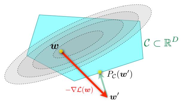
Figure 8.22: Illustration of projected gradient descent. w is the current parameter estimate, w^↓ is the update after a gradient step, and PC(w^↓ ) projects this onto the constraint set C. From https: // bit. ly/ 3eJ3BhZ Used with kind permission of Martin Jaggi.

elements if we don’t want to constrain values along that dimension. For example, if we just want to ensure the parameters are non-negative, we set l^d = 0 and u^d = ∈ for each dimension d.

We can convert the constrained optimization problem into an unconstrained one by adding a penalty term to the original objective:

\[ \mathcal{L}(\boldsymbol{\theta}) = \mathcal{L}\_s(\boldsymbol{\theta}) + \mathcal{L}\_r(\boldsymbol{\theta}) \tag{8.123} \]

where Lr(ω) is the indicator function for the convex set C, i.e.,

\[\mathcal{L}\_r(\boldsymbol{\theta}) = I\_{\mathcal{C}}(\boldsymbol{\theta}) = \begin{cases} 0 & \text{if } \boldsymbol{\theta} \in \mathcal{C} \\ \infty & \text{if } \boldsymbol{\theta} \notin \mathcal{C} \end{cases} \tag{8.124}\]

We can use proximal gradient descent to solve Equation (8.123). The proximal operator for the indicator function is equivalent to projection onto the set C:

\[\text{proj}\_{\mathcal{C}}(\boldsymbol{\theta}) = \underset{\boldsymbol{\theta}' \in \mathcal{C}}{\text{argmin}} ||\boldsymbol{\theta}' - \boldsymbol{\theta}||\_2 \tag{8.125}\]

This method is known as projected gradient descent. See Figure 8.22 for an illustration.

For example, consider the box constraints C = {ω : l ↘ ω ↘ u}. The projection operator in this case can be computed elementwise by simply thresholding at the boundaries:

\[\text{proj}\_{\mathcal{C}}(\boldsymbol{\theta})\_{d} = \begin{cases} l\_{d} & \text{if } \theta\_{d} \le l\_{d} \\ \theta\_{d} & \text{if } l\_{d} \le \theta\_{d} \le u\_{d} \\ u\_{d} & \text{if } \theta\_{d} \ge u\_{d} \end{cases} \tag{8.126}\]

For example, if we want to ensure all elements are non-negative, we can use

\[\text{proj}\_{\mathcal{C}}(\boldsymbol{\theta}) = \boldsymbol{\theta}\_{+} = [\max(\theta\_1, 0), \dots, \max(\theta\_D, 0)] \tag{8.127}\]

See Section 11.4.9.2 for an application of this method to sparse linear regression.

8.6.2 Proximal operator for ▷1-norm regularizer

Consider a linear predictor of the form f(x; ω) = $^{D d}=1 ϖdxd. If we have ϖ^d = 0 for any dimension d, we ignore the corresponding feature xd. This is a form of feature selection, which can be useful both as a way to reduce overfitting as well as way to improve model interpretability. We can encourage weights to be zero (and not just small) by penalizing the ω¹ norm,

\[||\theta||\_1 = \sum\_{d=1}^{D} |\theta\_d|\tag{8.128}\]

This is called a sparsity inducing regularizer.

To see why this induces sparsity, consider two possible parameter vectors, one which is sparse, ω = (1, 0), and one which is non-sparse, ω↗ = (1/ ^≃2, ¹/ ^≃2). Both have the same ^ω2 norm

\[||(1,0)||\_2^2 = ||(1/\sqrt{2}, 1/\sqrt{2})||\_2^2 = 1\tag{8.129}\]

Hence ω² regularization (Section 4.5.3) will not favor the sparse solution over the dense solution. However, when using ω¹ regularization, the sparse solution is cheaper, since

\[||(1,0)||\_1 = 1 < ||(1/\sqrt{2}, 1/\sqrt{2})||\_1 = \sqrt{2} \tag{8.130}\]

See Section 11.4 for more details on sparse regression.

If we combine this regularizer with our smooth loss, we get

\[\mathcal{L}(\theta) = \text{NLL}(\theta) + \lambda ||\theta||\_1 \tag{8.131}\]

We can optimize this objective using proximal gradient descent. The key question is how to compute the prox operator for the function f(ω) = ||ω||1. Since this function decomposes over dimensions d, the proximal projection can be computed componentwise. From Equation (8.120), with ◁ = 1, we have

\[\text{prox}\_{\lambda f}(\theta) = \operatorname\*{argmin}\_{z} |z| + \frac{1}{2\lambda} (z - \theta)^2 = \operatorname\*{argmin}\_{z} \lambda |z| + \frac{1}{2} (z - \theta)^2 \tag{8.132}\]

In Section 11.4.3, we show that the solution to this is given by

\[\text{prox}\_{\lambda f}(\theta) = \begin{cases} \theta - \lambda & \text{if } \theta \ge \lambda \\ 0 & \text{if } |\theta| \le \lambda \\ \theta + \lambda & \text{if } \theta \le -\lambda \end{cases} \tag{8.133}\]

This is known as the soft thresholding operator, since values less than φ in absolute value are set to 0 (thresholded), but in a continuous way. Note that soft thresholding can be written more compactly as

\[\text{SoftThreshold}(\theta, \lambda) = \text{sign}(\theta) \left( |\theta| - \lambda \right)\_{+} \tag{8.134}\]

where ϖ⁺ = max(ϖ, 0) is the positive part of ϖ. In the vector case, we perform this elementwise:

\[\text{SoftThreshold}(\theta, \lambda) = \text{sign}(\theta) \odot (|\theta| - \lambda)\_{+} \tag{8.135}\]

See Section 11.4.9.3 for an application of this method to sparse linear regression.

8.6.3 Proximal operator for quantization

In some applications (e.g., when training deep neural networks to run on memory-limited edge devices, such as mobile phones) we want to ensure that the parameters are quantized. For example, in the extreme case where each parameter can only be -1 or +1, the state space becomes ^{C =} {↑1, +1}D.

Let us define a regularizer that measures distance to the nearest quantized version of the parameter vector:

\[\mathcal{L}\_r(\boldsymbol{\theta}) = \inf\_{\boldsymbol{\theta}\_0 \in \mathcal{C}} ||\boldsymbol{\theta} - \boldsymbol{\theta}\_0||\_1 \tag{8.136}\]

(We could also use the ^ω2 norm.) In the case of ^{C =} {↑1, +1}^D, this becomes

\[\mathcal{L}\_r(\boldsymbol{\theta}) = \sum\_{d=1}^D \inf\_{\{\theta\_0\}\_d \in \{\pm 1\}} |\theta\_d - [\theta\_0]\_d| = \sum\_{d=1}^D \min\{ |\theta\_d - 1|, |\theta\_d + 1| \} = ||\boldsymbol{\theta} - \text{sign}(\boldsymbol{\theta})||\_1 \tag{8.137}\]

Let us define the corresponding quantization operator to be

\[q(\boldsymbol{\theta}) = \text{proj}\_{\mathbb{C}}(\boldsymbol{\theta}) = \operatorname\*{argmin}\_{r} \mathcal{L}\_{r}(\boldsymbol{\theta}) = \text{sign}(\boldsymbol{\theta})\tag{8.138}\]

The core di”culty with quantized learning is that quantization is not a di!erentiable operation. A popular solution to this is to use the straight-through estimator, which uses the approximation ϖL ^ϖq(ω) ↖ ^{ϖL ϖω} (see e.g., [Yin+19]). The corresponding update can be done in two steps: first compute the gradient vector at the quantized version of the current parameters, and then update the unconstrained parameters using this approximate gradient:

\[\dot{\boldsymbol{\theta}}\_{t} = \text{proj}\_{\mathcal{C}}(\boldsymbol{\theta}\_{t}) = q(\boldsymbol{\theta}\_{t}) \tag{8.139}\]

\[ \theta\_{t+1} = \theta\_t - \eta\_t \nabla \mathcal{L}\_s(\tilde{\theta}\_t) \tag{8.140} \]

When applied to ^{C =} {↑1, +1}^D, this is known as the binary connect method [CBD15].

We can get better results using proximal gradient descent, in which we treat quantization as a regularizer, rather than a hard constraint; this is known as ProxQuant [BWL19]. The update becomes

\[\dot{\boldsymbol{\theta}}\_{t} = \text{prox}\_{\lambda \mathcal{L}\_{r}} \left( \boldsymbol{\theta}\_{t} - \eta\_{t} \nabla \mathcal{L}\_{s}(\boldsymbol{\theta}\_{t}) \right) \tag{8.141}\]

In the case that ^{C =} {↑1, +1}^D, one can show that the proximal operator is a generalization of the soft thresholding operator in Equation (8.135):

\[\text{prox}\_{\lambda \mathcal{L}\_r}(\boldsymbol{\theta}) = \text{SoftThreshold}(\boldsymbol{\theta}, \lambda, \text{sign}(\boldsymbol{\theta})) \tag{8.142}\]

\[=\text{sign}(\theta) + \text{sign}(\theta - \text{sign}(\theta)) \odot (|\theta - \text{sign}(\theta)| - \lambda)\_{+} \tag{8.143}\]

This can be generalized to other forms of quantization; see [Yin+19] for details.

8.6.4 Incremental (online) proximal methods

Many ML problems have an objective function which is a sum of losses, one per example. Such problems can be solved incrementally; this is a special case of online learning. It is possible to extend proximal methods to this setting. For a probabilistic perspective on such methods (in terms of Kalman filtering), see [AEM18; Aky+19].

8.7 Bound optimization *

In this section, we consider a class of algorithms known as bound optimization or MM algorithms. In the context of minimization, MM stands for majorize-minimize. In the context of maximization, MM stands for minorize-maximize. We will discuss a special case of MM, known as expectation maximization or EM, in Section 8.7.2.

8.7.1 The general algorithm

In this section, we give a brief outline of MM methods. (More details can be found in e.g., [HL04; Mai15; SBP17; Nad+19].) To be consistent with the literature, we assume our goal is to maximize some function ω(ω), such as the log likelihood, wrt its parameters ω. The basic approach in MM algorithms is to construct a surrogate function Q(ω, ω^t ) which is a tight lowerbound to ω(ω) such that Q(ω, ω^t ) ↘ ^ω(ω) and ^Q(ω^t , ω^t ) = ω(ω^t ). If these conditions are met, we say that Q minorizes ω. We then perform the following update at each step:

\[\theta^{t+1} = \underset{\theta}{\text{argmax}} \, Q(\theta, \theta^t) \tag{8.144}\]

This guarantees us monotonic increases in the original objective:

\[\ell(\theta^{t+1}) \ge Q(\theta^{t+1}, \theta^t) \ge Q(\theta^t, \theta^t) = \ell(\theta^t) \tag{8.145}\]

where the first inequality follows since Q(ω^t+1, ω↗ ) is a lower bound on ω(ω^t+1) for any ω↗ ; the second inequality follows from Equation (8.144); and the final equality follows the tightness property. As a consequence of this result, if you do not observe monotonic increase of the objective, you must have an error in your math and/or code. This is a surprisingly powerful debugging tool.

This process is sketched in Figure 8.23. The dashed red curve is the original function (e.g., the log-likelihood of the observed data). The solid blue curve is the lower bound, evaluated at ω^t ; this touches the objective function at ω^t . We then set ω^t+1 to the maximum of the lower bound (blue curve), and fit a new bound at that point (dotted green curve). The maximum of this new bound becomes ω^t+2, etc.

If Q is a quadratic lower bound, the overall method is similar to Newton’s method, which repeatedly fits and then optimizes a quadratic approximation, as shown in Figure 8.14(a). The di!erence is that optimizing Q is guaranteed to lead to an improvement in the objective, even if it is not convex, whereas Newton’s method may overshoot or lead to a decrease in the objective, as shown in Figure 8.24, since it is a quadratic approximation and not a bound.

8.7.2 The EM algorithm

In this section, we discuss the expectation maximization (EM) algorithm [DLR77; MK97], which is a bound optimization algorithm designed to compute the MLE or MAP parameter estimate for probability models that have missing data and/or hidden variables. We let yⁿ be the visible data for example n, and zⁿ be the hidden data.

The basic idea behind EM is to alternate between estimating the hidden variables (or missing values) during the E step (expectation step), and then using the fully observed data to compute the MLE during the M step (maximization step). Of course, we need to iterate this process, since the expected values depend on the parameters, but the parameters depend on the expected values.

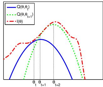
Figure 8.23: Illustration of a bound optimization algorithm. Adapted from Figure 9.14 of [Bis06]. Generated by emLogLikelihoodMax.ipynb.

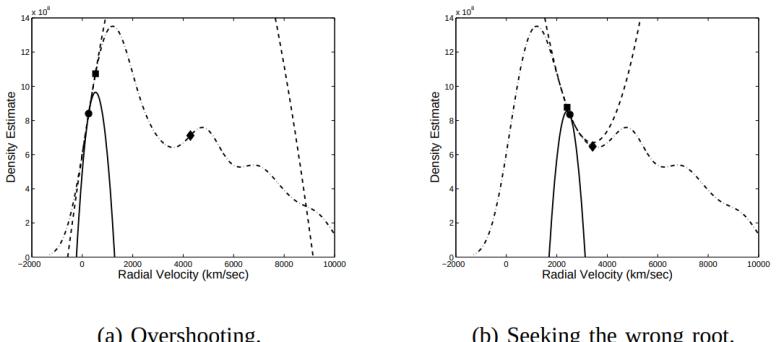
Figure 8.24: The quadratic lower bound of an MM algorithm (solid) and the quadratic approximation of Newton’s method (dashed) superimposed on an empirical density esitmate (dotted). The starting point of both algorithms is the circle. The square denotes the outcome of one MM update. The diamond denotes the outcome of one Newton update. (a) Newton’s method overshoots the global maximum. (b) Newton’s method results in a reduction of the objective. From Figure 4 of [FT05]. Used with kind permission of Carlo Tomasi.

In Section 8.7.2.1, we show that EM is an MM algorithm, which implies that this iterative procedure will converge to a local maximum of the log likelihood. The speed of convergence depends on the amount of missing data, which a!ects the tightness of the bound [XJ96; MD97; SRG03; KKS20].

8.7.2.1 Lower bound

The goal of EM is to maximize the log likelihood of the observed data:

\[\ell(\boldsymbol{\theta}) = \sum\_{n=1}^{N} \log p(y\_n|\boldsymbol{\theta}) = \sum\_{n=1}^{N} \log \left[ \sum\_{z\_n} p(y\_n, z\_n|\boldsymbol{\theta}) \right] \tag{8.146}\]

where yⁿ are the visible variables and zⁿ are the hidden variables. Unfortunately this is hard to optimize, since the log cannot be pushed inside the sum.

EM gets around this problem as follows. First, consider a set of arbitrary distributions qn(zn) over each hidden variable zn. The observed data log likelihood can be written as follows:

\[\ell(\boldsymbol{\theta}) = \sum\_{n=1}^{N} \log \left[ \sum\_{\mathbf{z}\_n} q\_n(\mathbf{z}\_n) \frac{p(\mathbf{y}\_n, \mathbf{z}\_n | \boldsymbol{\theta})}{q\_n(\mathbf{z}\_n)} \right] \tag{8.147}\]

Using Jensen’s inequality (Equation (6.34)), we can push the log (which is a concave function) inside the expectation to get the following lower bound on the log likelihood:

\[\ell(\boldsymbol{\theta}) \ge \sum\_{n} \sum\_{\mathbf{z}\_n} q\_n(\mathbf{z}\_n) \log \frac{p(\mathbf{y}\_n, \mathbf{z}\_n | \boldsymbol{\theta})}{q\_n(\mathbf{z}\_n)} \tag{8.148}\]

\[\mathbb{E}\_{n} = \sum\_{n} \underbrace{\mathbb{E}\_{q\_{n}} \left[ \log p(\mathbf{y}\_{n}, \mathbf{z}\_{n} | \boldsymbol{\theta}) \right] + \mathbb{H}(q\_{n})}\_{\mathbb{L}(\boldsymbol{\theta}, q\_{n})} \tag{8.149}\]

\[\mathbf{h} = \sum\_{n} \mathbf{L}(\boldsymbol{\theta}, q\_n) \stackrel{\scriptstyle}{=} \mathbf{L}(\boldsymbol{\theta}, \{q\_n\}) = \mathbf{L}(\boldsymbol{\theta}, q\_{1:N}) \tag{8.150}\]

where H(q) is the entropy of probability distribution q, and $(ω, {qn}) is called the evidence lower bound or ELBO, since it is a lower bound on the log marginal likelihood, log p(y1:^N |ω), also called the evidence. Optimizing this bound is the basis of variational inference, which we discuss in Section 4.6.8.3.

8.7.2.2 E step

We see that the lower bound is a sum of N terms, each of which has the following form:

\[\text{KL}(\theta, q\_n) = \sum\_{\mathbf{z}\_n} q\_n(\mathbf{z}\_n) \log \frac{p(y\_n, \mathbf{z}\_n | \theta)}{q\_n(\mathbf{z}\_n)} \tag{8.151}\]

\[\hat{\mathbf{y}} = \sum\_{\mathbf{z}\_n} q\_n(\mathbf{z}\_n) \log \frac{p(\mathbf{z}\_n | \mathbf{y}\_n, \boldsymbol{\theta}) p(\mathbf{y}\_n | \boldsymbol{\theta})}{q\_n(\mathbf{z}\_n)} \tag{8.152}\]

\[\hat{\mathbf{y}} = \sum\_{\mathbf{z}\_n} q\_n(\mathbf{z}\_n) \log \frac{p(\mathbf{z}\_n | \mathbf{y}\_n, \boldsymbol{\theta})}{q\_n(\mathbf{z}\_n)} + \sum\_{\mathbf{z}\_n} q\_n(\mathbf{z}\_n) \log p(\mathbf{y}\_n | \boldsymbol{\theta}) \tag{8.153}\]

\[=-D\_{\rm KL}\left(q\_n(\mathbf{z}\_n)\parallel p(\mathbf{z}\_n|\mathbf{y}\_n,\boldsymbol{\theta})\right) + \log p(\mathbf{y}\_n|\boldsymbol{\theta})\tag{8.154}\]

where ^DKL (^{q 7 p}) ↭ $ ^{z q}(z)log ^q(z) ^p(z) is the Kullback-Leibler divergence (or KL divergence for short) between probability distributions q and p. We discuss this in more detail in Section 6.2, but the key property we need here is that DKL (q 7 p) ∋ 0 and DKL (q 7 p) = 0 i! q = p. Hence we can maximize the lower bound $(ω, {qn}) wrt {qn} by setting each one to q^{↓ n} = p(zn|yn, ω). This is called the E step. This ensures the ELBO is a tight lower bound:

\[\mathbb{E}(\boldsymbol{\theta}, \{q\_n^\*\}) = \sum\_n \log p(y\_n|\boldsymbol{\theta}) = \ell(\boldsymbol{\theta}) \tag{8.155}\]

To see how this connects to bound optimization, let us define

\[Q(\theta, \theta^t) = \mathbb{L}(\theta, \{p(\mathbf{z}\_n | y\_n; \theta^t)\}) \tag{8.156}\]

Then we have Q(ω, ω^t ) ↘ ^ω(ω) and ^Q(ω^t , ω^t ) = ω(ω^t ), as required.

However, if we cannot compute the posteriors ^p(zn|yn; ^ωt ) exactly, we can still use an approximate distribution ^q(zn|yn; ^ωt ); this will yield a non-tight lower-bound on the log-likelihood. This generalized version of EM is known as variational EM [NH98]. See the sequel to this book, [Mur23], for details.

8.7.2.3 M step

In the M step, we need to maximize $(ω, {q^{t n}}) wrt ^ω, where the ^{qt n} are the distributions computed in the E step at iteration t. Since the entropy terms H(qn) are constant wrt ω, so we can drop them in the M step. We are left with

\[\ell^t(\boldsymbol{\theta}) = \sum\_{n} \mathbb{E}\_{q\_n^t(\mathbf{z}\_n)} \left[ \log p(y\_n, \mathbf{z}\_n | \boldsymbol{\theta}) \right] \tag{8.157}\]

This is called the expected complete data log likelihood. If the joint probability is in the exponential family (Section 3.4), we can rewrite this as

\[\ell^t(\boldsymbol{\theta}) = \sum\_{n} \mathbb{E}\left[\mathcal{T}(\boldsymbol{y}\_n, \mathbf{z}\_n)^\mathsf{T} \boldsymbol{\theta} - A(\boldsymbol{\theta})\right] = \sum\_{n} \left(\mathbb{E}\left[\mathcal{T}(\boldsymbol{y}\_n, \mathbf{z}\_n)\right]^\mathsf{T} \boldsymbol{\theta} - A(\boldsymbol{\theta})\right) \tag{8.158}\]

where E [T (yn, zn)] are called the expected su!cient statistics.

In the M step, we maximize the expected complete data log likelihood to get

\[\boldsymbol{\theta}^{t+1} = \arg\max\_{\boldsymbol{\theta}} \sum\_{n} \mathbb{E}\_{q\_n^t} \left[ \log p(y\_n, z\_n | \boldsymbol{\theta}) \right] \tag{8.159}\]

In the case of the exponential family, the maximization can be solved in closed-form by matching the moments of the expected su”cient statistics.

We see from the above that the E step does not in fact need to return the full set of posterior distributions $ {q(zn)}, but can instead just return the sum of the expected su”cient statistics, ⁿ Eq(zn) [T (yn, zn)]. This will become clearer in the examples below.

8.7.3 Example: EM for a GMM

In this section, we show how to use the EM algorithm to compute MLE and MAP estimates of the parameters for a Gaussian mixture model (GMM).

8.7.3.1 E step

The E step simply computes the responsibility of cluster k for generating data point n, as estimated using the current parameter estimates ω(t) :

\[r\_{nk}^{(t)} = p^\*(z\_n = k | \mathbf{y}\_n, \boldsymbol{\theta}^{(t)}) = \frac{\pi\_k^{(t)} p(\mathbf{y}\_n | \boldsymbol{\theta}\_k^{(t)})}{\sum\_{k'} \pi\_{k'}^{(t)} p(\mathbf{y}\_n | \boldsymbol{\theta}\_{k'}^{(t)})} \tag{8.160}\]

8.7.3.2 M step

The M step maximizes the expected complete data log likelihood, given by

\[\ell^t(\boldsymbol{\theta}) = \mathbb{E}\left[\sum\_{n} \log p(z\_n|\boldsymbol{\pi}) + \sum\_{n} \log p(y\_n|z\_n, \boldsymbol{\theta})\right] \tag{8.161}\]

\[=\mathbb{E}\left[\sum\_{n}\log\left(\prod\_{k}\pi\_{k}^{z\_{nk}}\right)+\sum\_{n}\log\left(\prod\_{k}\mathcal{N}(y\_{n}|\boldsymbol{\mu}\_{k},\boldsymbol{\Sigma}\_{k})^{z\_{nk}}\right)\right]\tag{8.162}\]

\[\hat{\mu} = \sum\_{n} \sum\_{k} \mathbb{E}\left[z\_{nk}\right] \log \pi\_{k} + \sum\_{n} \sum\_{k} \mathbb{E}\left[z\_{nk}\right] \log \mathcal{N}(y\_{n}|\mu\_{k}, \Sigma\_{k}) \tag{8.163}\]

\[\hat{\rho} = \sum\_{n} \sum\_{k} r\_{nk}^{(t)} \log(\pi\_k) - \frac{1}{2} \sum\_{n} \sum\_{k} r\_{nk}^{(t)} \left[ \log |\boldsymbol{\Sigma}\_k| + (\boldsymbol{y}\_n - \boldsymbol{\mu}\_k)^\mathsf{T} \boldsymbol{\Sigma}\_k^{-1} (\boldsymbol{y}\_n - \boldsymbol{\mu}\_k) \right] + \text{const} \tag{8.164}\]

where znk = I(zⁿ = k) is a one-hot encoding of the categorical value zn. This objective is just a weighted version of the standard problem of computing the MLEs of an MVN (see Section 4.2.6). One can show that the new parameter estimates are given by

\[\begin{split} \boldsymbol{\mu}\_{k}^{(t+1)} &= \frac{\sum\_{n} r\_{nk}^{(t)} \mathbf{y}\_{n}}{r\_{k}^{(t)}} \\ \boldsymbol{\Sigma}\_{k}^{(t+1)} &= \frac{\sum\_{n} r\_{nk}^{(t)} (\mathbf{y}\_{n} - \boldsymbol{\mu}\_{k}^{(t+1)}) (\mathbf{y}\_{n} - \boldsymbol{\mu}\_{k}^{(t+1)})^{\mathsf{T}}}{r\_{k}^{(t)}} \\ &= \frac{\sum\_{n} r\_{nk}^{(t)} \mathbf{y}\_{n} \mathbf{y}\_{n}^{\mathsf{T}}}{r\_{k}^{(t)}} - \boldsymbol{\mu}\_{k}^{(t+1)} (\boldsymbol{\mu}\_{k}^{(t+1)})^{\mathsf{T}} \end{split} \tag{8.166}\]

where r (t) ^k ↭ $ n r (t) nk is the weighted number of points assigned to cluster k. The mean of cluster k is just the weighted average of all points assigned to cluster k, and the covariance is proportional to the weighted empirical scatter matrix.

The M step for the mixture weights is simply a weighted form of the usual MLE:

\[\pi\_k^{(t+1)} = \frac{1}{N} \sum\_n r\_{nk}^{(t)} = \frac{r\_k^{(t)}}{N} \tag{8.167}\]

8.7.3.3 Example

An example of the algorithm in action is shown in Figure 8.25 where we fit some 2d data with a 2 component GMM. The data set, from [Bis06], is derived from measurements of the Old Faithful geyser in Yellowstone National Park. In particular, we plot the time to next eruption in minutes versus the duration of the eruption in minutes. The data was standardized, by removing the mean and dividing by the standard deviation, before processing; this often helps convergence. We start with µ¹ = (↑1, 1), !¹ = I, µ² = (1, ↑1), !² = I. We then show the cluster assignments, and corresponding mixture components, at various iterations.

For more details on applying GMMs for clustering, see Section 21.4.1.

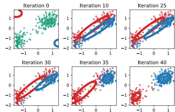
Figure 8.25: Illustration of the EM for a GMM applied to the Old Faithful data. The degree of redness indicates the degree to which the point belongs to the red cluster, and similarly for blue; thus purple points have a roughly 50/50 split in their responsibilities to the two clusters. Adapted from [Bis06] Figure 9.8. Generated by mix\_gauss\_demo\_faithful.ipynb.

8.7.3.4 MAP estimation

Computing the MLE of a GMM often su!ers from numerical problems and overfitting. To see why, suppose for simplicity that !^k = ε^{2 k}I for all k. It is possible to get an infinite likelihood by assigning one of the centers, say µk, to a single data point, say yn, since then the likelihood of that data point is given by

\[N(y\_n | \mu\_k = y\_n, \sigma\_k^2 \mathbf{I}) = \frac{1}{\sqrt{2\pi\sigma\_k^2}} e^0 \tag{8.168}\]

Hence we can drive this term to infinity by letting ε^k ↔︎ 0, as shown in Figure 8.26(a). We call this the “collapsing variance problem”.

An easy solution to this is to perform MAP estimation. Fortunately, we can still use EM to find this MAP estimate. Our goal is now to maximize the expected complete data log-likelihood plus the log prior:

\[\ell^t(\boldsymbol{\theta}) = \left[ \sum\_{n} \sum\_{k} r\_{nk}^{(t)} \log \pi\_{nk} + \sum\_{n} \sum\_{k} r\_{nk}^{(t)} \log p(\mathbf{y}\_n | \boldsymbol{\theta}\_k) \right] + \log p(\boldsymbol{\pi}) + \sum\_{k} \log p(\boldsymbol{\theta}\_k) \tag{8.169}\]

Note that the E step remains unchanged, but the M step needs to be modified, as we now explain.

For the prior on the mixture weights, it is natural to use a Dirichlet prior (Section 4.6.3.2), ς ⇒ Dir(φ), since this is conjugate to the categorical distribution. The MAP estimate is given by

\[ \hat{\pi}\_k^{(t+1)} = \frac{r\_k^{(t)} + \alpha\_k - 1}{N + \sum\_k \alpha\_k - K} \tag{8.170} \]

If we use a uniform prior, ϱ^k = 1, this reduces to the MLE.

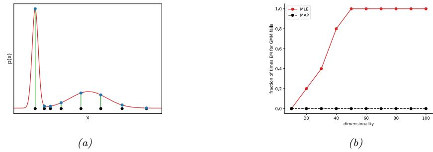
Figure 8.26: (a) Illustration of how singularities can arise in the likelihood function of GMMs. Here K = 2, but the first mixture component is a narrow spike (with ϑ¹ ∞ 0) centered on a single data point x1. Adapted from Figure 9.7 of [Bis06]. Generated by mix\_gauss\_singularity.ipynb. (b) Illustration of the benefit of MAP estimation vs ML estimation when fitting a Gaussian mixture model. We plot the fraction of times (out of 5 random trials) each method encounters numerical problems vs the dimensionality of the problem, for N = 100 samples. Solid red (upper curve): MLE. Dotted black (lower curve): MAP. Generated by mix\_gauss\_mle\_vs\_map.ipynb.

For the prior on the mixture components, let us consider a conjugate prior of the form

\[p(\mu\_k, \Sigma\_k) = \text{NIW}(\mu\_k, \Sigma\_k \mid \check{\mathbf{m}}, \mathbb{X}, \mathbb{Y}, \check{\mathbf{S}}) \tag{8.171}\]

This is called the Normal-Inverse-Wishart distribution (see the sequel to this book, [Mur23], for details.) Suppose we set the hyper-parameters for µ to be ↫2= 0, so that the µ^k are unregularized; thus the prior will only influence our estimate of !k. In this case, the MAP estimates are given by

\[ \hat{\boldsymbol{\mu}}\_{k}^{(t+1)} = \hat{\boldsymbol{\mu}}\_{k}^{(t+1)} \tag{8.172} \]

\[\dot{\boldsymbol{\Sigma}}\_{k}^{(t+1)} = \frac{\check{\mathbf{S}} + \hat{\mathbf{E}}\_{k}^{(t+1)}}{\mathbb{V} + r\_{k}^{(t)} + D + 2} \tag{8.173}\]

where µˆ^k is the MLE for µ^k from Equation (8.165), and !ˆ ^k is the MLE for !^k from Equation (8.166).

Now we discuss how to set the prior covariance, ↫ S. One possibility (suggested in [FR07, p163]) is to use

\[\check{\mathbf{S}} = \frac{1}{K^{2/D}} \text{diag}(s\_1^2, \dots, s\_D^2) \tag{8.174}\]

where s^{2 d} = (1/N) $^{N n}=1(xnd ^↑xd)² is the pooled variance for dimension ^d. The parameter ↫⇀ controls how strongly we believe this prior. The weakest prior we can use, while still being proper, is to set ↫⇀= D + 2, so this is a common choice.

We now illustrate the benefits of using MAP estimation instead of ML estimation in the context of GMMs. We apply EM to some synthetic data with N = 100 samples in D dimensions, using either ML or MAP estimation. We count the trial as a “failure” if there are numerical issues involving singular matrices. For each dimensionality, we conduct 5 random trials. The results are illustrated in Figure 8.26(b). We see that as soon as D becomes even moderately large, ML estimation crashes and burns, whereas MAP with an appropriate prior estimation rarely encounters numerical problems.

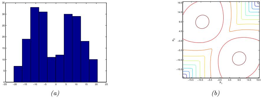
Figure 8.27: Left: N = 200 data points sampled from a mixture of 2 Gaussians in 1d, with ς^k = 0.5, ϑ^k = 5, µ¹ = ↑10 and µ² = 10. Right: Likelihood surface p(D|µ1, µ2), with all other parameters set to their true values. We see the two symmetric modes, reflecting the unidentifiability of the parameters. Generated by gmm\_lik\_surface\_plot.ipynb.

8.7.3.5 Nonconvexity of the NLL

The likelihood for a mixture model is given by

\[\ell(\theta) = \sum\_{n=1}^{N} \log \left[ \sum\_{z\_n=1}^{K} p(y\_n, z\_n | \theta) \right] \tag{8.175}\]

In general, this will have multiple modes, and hence there will not be a unique global optimum.

Figure 8.27 illustrates this for a mixture of 2 Gaussians in 1d. We see that there are two equally good global optima, corresponding to two di!erent labelings of the clusters, one in which the left peak corresponds to z = 1, and one in which the left peak corresponds to z = 2. This is called the label switching problem; see Section 21.4.1.2 for more details.

The question of how many modes there are in the likelihood function is hard to answer. There are K! possible labelings, but some of the peaks might get merged, depending on how far apart the µ^k are. Nevertheless, there can be an exponential number of modes. Consequently, finding any global optimum is NP-hard [Alo+09; Dri+04]. We will therefore have to be satisfied with finding a local optimum. To find a good local optimum, we can use Kmeans++ (Section 21.3.4) to initialize EM.

8.8 Blackbox and derivative free optimization

In some optimization problems, the objective function is a blackbox, meaning that its functional form is unknown. This means we cannot use gradient-based methods to optimize it. Instead, solving such problems require blackbox optimization (BBO) methods, also called derivative free optimization (DFO).

In ML, this kind of problem often arises when performing model selection. For example, suppose we have some hyper-parameters, ϱ → “, which control the type or complexity of a model. We often define the objective function L(ϱ) to be the loss on a validation set (see Section 4.5.4). Since the validation loss depends on the optimal model parameters, which are computed using a complex algorithm, this objective function is e!ectively a blackbox.4

A simple approach to such problems is to use grid search, where we evaluate each point in the parameter space, and pick the one with the lowest loss. Unfortunately, this does not scale to high dimensions, because of the curse of dimensionality. In addition, even in low dimensions this can be expensive if evaluating the blackbox objective is expensive (e.g., if it first requires training the model before computing the validation loss). Various solutions to this problem have been proposed. See the sequel to this book, [Mur23], for details.

8.9 Exercises

Exercise 8.1 [Subderivative of the hinge loss function † ]

Let f(x) = (1 ↑ x)⁺ be the hinge loss function, where (z)⁺ = max(0, z). What are 0f(0), 0f(1), and 0f(2)?

Exercise 8.2 [EM for the Student distribution]

Derive the EM equations for computing the MLE for a multivariate Student distribution. Consider the case where the dof parameter is known and unknown separately. Hint: write the Student distribution as a scale mixture of Gaussians.

^4. If the optimal parameters are computed using a gradient-based optimizer, we can “unroll” the gradient steps, to create a deep circuit that maps from the training data to the optimal parameters and hence to the validation loss. We can then optimize through the optimizer (see e.g., [Fra+17]). However, this technique can only be applied in limited settings.

Part II

Linear Models

9 Linear Discriminant Analysis

9.1 Introduction

In this chapter, we consider classification models of the following form:

\[p(y=c|\mathbf{x}, \boldsymbol{\theta}) = \frac{p(\mathbf{x}|y=c, \boldsymbol{\theta})p(y=c|\boldsymbol{\theta})}{\sum\_{c'} p(\mathbf{x}|y=c', \boldsymbol{\theta})p(y=c'|\boldsymbol{\theta})} \tag{9.1}\]

The term p(y = c|ω) is the prior over class labels, and the term p(x|y = c, ω) is called the class conditional density for class c.

The overall model is called a generative classifier, since it specifies a way to generate the features x for each class c, by sampling from p(x|y = c, ω). By contrast, a discriminative classifier directly models the class posterior p(y|x, ω). We discuss the pros and cons of these two approaches to classification in Section 9.4.

If we choose the class conditional densities in a special way, we will see that the resulting posterior over classes is a linear function of ^x, i.e., log ^p(^{y = c}|x, ^ω) = ^{wTx +} const, where ^w is derived from ω. Thus the overall method is called linear discriminant analysis or LDA. 1

9.2 Gaussian discriminant analysis

In this section, we consider a generative classifier where the class conditional densities are multivariate Gaussians:

\[p(x|y=c,\theta) = N(x|\mu\_c, \Sigma\_c) \tag{9.2}\]

The corresponding class posterior therefore has the form

\[p(y = c | \mathbf{x}, \boldsymbol{\theta}) \propto \pi\_c \mathcal{N}(\boldsymbol{x} | \boldsymbol{\mu}\_c, \boldsymbol{\Sigma}\_c) \tag{9.3}\]

where ϑ^c = p(y = c|ω) is the prior probability of label c. (Note that we can ignore the normalization constant in the denominator of the posterior, since it is independent of c.) We call this model Gaussian discriminant analysis or GDA.

^1. This term is rather confusing for two reasons. First, LDA is a generative, not discriminative, classifier. Second, LDA also stands for “latent Dirichlet allocation”, which is a popular unsupervised generative model for bags of words [BNJ03].

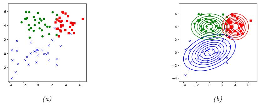
Figure 9.1: (a) Some 2d data from 3 di!erent classes. (b) Fitting 2d Gaussians to each class. Generated by discrim\_analysis\_dboundaries\_plot2.ipynb.

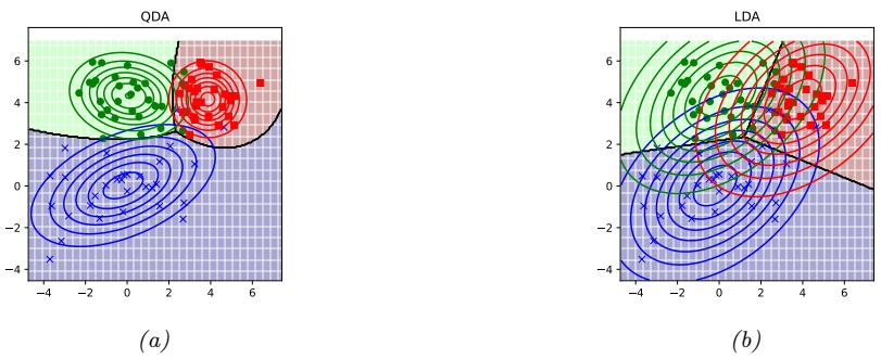
Figure 9.2: Gaussian discriminant analysis fit to data in Figure 9.1. (a) Unconstrained covariances induce quadratic decision boundaries. (b) Tied covariances induce linear decision boundaries. Generated by discrim\_analysis\_dboundaries\_plot2.ipynb.

9.2.1 Quadratic decision boundaries

From Equation (9.3), we see that the log posterior over class labels is given by

\[\log p(y = c | \mathbf{z}, \boldsymbol{\theta}) = \log \pi\_c - \frac{1}{2} \log |2\pi\Sigma\_c| - \frac{1}{2} (\boldsymbol{x} - \boldsymbol{\mu}\_c)^\mathsf{T} \boldsymbol{\Sigma}\_c^{-1} (\boldsymbol{x} - \boldsymbol{\mu}\_c) + \text{const} \tag{9.4}\]

This is called the discriminant function. We see that the decision boundary between any two classes, say c and c↗ , will be a quadratic function of x. Hence this is known as quadratic discriminant analysis (QDA).

For example, consider the 2d data from 3 di!erent classes in Figure 9.1a. We fit full covariance Gaussian class-conditionals (using the method explained in Section 9.2.4), and plot the results in Figure 9.1b. We see that the features for the blue class are somewhat correlated, whereas the features for the green class are independent, and the features for the red class are independent and isotropic (spherical covariance). In Figure 9.2a, we see that the resulting decision boundaries are quadratic functions of x.

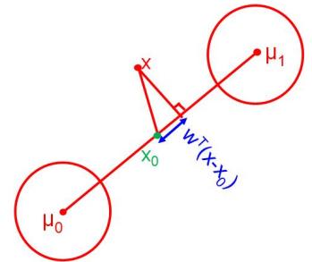
Figure 9.3: Geometry of LDA in the 2 class case where !¹ = !² = I.

9.2.2 Linear decision boundaries

Now we consider a special case of Gaussian discriminant analysis in which the covariance matrices are tied or shared across classes, so !^c = !. If ! is independent of c, we can simplify Equation (9.4) as follows:

\[\log p(y = c | \mathbf{x}, \boldsymbol{\theta}) = \log \pi\_c - \frac{1}{2} (\boldsymbol{x} - \boldsymbol{\mu}\_c)^\mathsf{T} \boldsymbol{\Sigma}^{-1} (\boldsymbol{x} - \boldsymbol{\mu}\_c) + \text{const} \tag{9.5}\]

\[\xi = \underbrace{\log \pi\_c - \frac{1}{2} \mu\_c^\mathrm{T} \Sigma^{-1} \mu\_c}\_{\gamma\_c} + x^\mathrm{T} \underbrace{\Sigma^{-1} \mu\_c}\_{\beta\_c} + \text{const} - \frac{1}{2} x^\mathrm{T} \Sigma^{-1} x}\_{\kappa} \tag{9.6}\]

\[ \hat{\rho} = \gamma\_c + \boldsymbol{x}^{\mathsf{T}} \boldsymbol{\beta}\_c + \kappa \tag{9.7} \]

The final term is independent of c, and hence is an irrelevant additive constant that can be dropped. Hence we see that the discriminant function is a linear function of x, so the decision boundaries will be linear. Hence this method is called linear discriminant analysis or LDA. See Figure 9.2b for an example.

9.2.3 The connection between LDA and logistic regression

In this section, we derive an interesting connection between LDA and logistic regression, which we introduced in Section 2.5.3. From Equation (9.7) we can write

\[p(y = c | \mathbf{z}, \boldsymbol{\theta}) = \frac{e^{\mathcal{B}\_c^\mathsf{T} \mathbf{z} + \gamma\_c}}{\sum\_{c'} e^{\mathcal{B}\_{c'}^\mathsf{T} \mathbf{z} + \gamma\_{c'}}} = \frac{e^{\mathbf{w}\_c^\mathsf{T}[1, \mathbf{z}]}}{\sum\_{c'} e^{\mathbf{w}\_{c'}^\mathsf{T}[1, \mathbf{z}]}} \tag{9.8}\]

where w^c = [⇁c, εc]. We see that Equation (9.8) has the same form as the multinomial logistic regression model. The key di!erence is that in LDA, we first fit the Gaussians (and class prior) to maximize the joint likelihood p(x, y|ω), as discussed in Section 9.2.4, and then we derive w from ω. By contrast, in logistic regression, we estimate w directly to maximize the conditional likelihood p(y|x, w). In general, these can give di!erent results (see Exercise 10.3).

To gain further insight into Equation (9.8), let us consider the binary case. In this case, the

posterior is given by

\[p(y=1|\mathbf{z},\boldsymbol{\theta}) = \frac{e^{\beta\_1^{\mathsf{T}}\mathbf{z} + \gamma\_1}}{e^{\beta\_1^{\mathsf{T}}\mathbf{z} + \gamma\_1} + e^{\beta\_0^{\mathsf{T}}\mathbf{z} + \gamma\_0}} = \frac{1}{1 + e^{(\beta\_0 - \beta\_1)^{\mathsf{T}}\mathbf{z} + (\gamma\_0 - \gamma\_1)}}\tag{9.9}\]

\[\sigma = \sigma \left( (\beta\_1 - \beta\_0)^\mathsf{T} x + (\gamma\_1 - \gamma\_0) \right) \tag{9.10}\]

where ε(◁) refers to the sigmoid function.

Now

\[ \gamma\_1 - \gamma\_0 = -\frac{1}{2} \mu\_1^\mathsf{T} \Sigma^{-1} \mu\_1 + \frac{1}{2} \mu\_0^\mathsf{T} \Sigma^{-1} \mu\_0 + \log(\pi\_1/\pi\_0) \tag{9.11} \]

\[=-\frac{1}{2}(\mu\_1-\mu\_0)^\mathsf{T}\Sigma^{-1}(\mu\_1+\mu\_0)+\log(\pi\_1/\pi\_0)\tag{9.12}\]

So if we define

\[ \Delta w = \beta\_1 - \beta\_0 = \Sigma^{-1} (\mu\_1 - \mu\_0) \tag{9.13} \]

\[x\_0 = \frac{1}{2}(\mu\_1 + \mu\_0) - (\mu\_1 - \mu\_0)\frac{\log(\pi\_1/\pi\_0)}{(\mu\_1 - \mu\_0)^\mathsf{T}\Sigma^{-1}(\mu\_1 - \mu\_0)}\tag{9.14}\]

then we have ^wTx^{0 = ↑}(⇁^{1 ↑} ⇁0), and hence

\[p(y=1|x,\theta) = \sigma(w^{\mathsf{T}}(x-x\_0))\tag{9.15}\]

This has the same form as binary logistic regression. Hence the MAP decision rule is

\[\hat{y}(\mathbf{x}) = 1 \text{ iff } \mathbf{w}^{\mathsf{T}} \mathbf{x} > c \tag{9.16}\]

where c = w^Tx0. If ϑ⁰ = ϑ¹ = 0.5, then the threshold simplifies to c = ^{1 2}w^T(µ¹ + µ0).

To interpret this equation geometrically, suppose ! = ^ε2I. In this case, ^w = ^ε→²(µ^{1 ↑ µ}0), which is parallel to a line joining the two centroids, µ⁰ and µ1. So we can classify a point by projecting it onto this line, and then checking if the projection is closer to µ⁰ or µ1, as illustrated in Figure 9.3. The question of how close it has to be depends on the prior over classes. If ϑ¹ = ϑ0, then x⁰ = ^{1 2} (µ¹ + µ0), which is halfway between the means. If we make ϑ¹ > ϑ0, we have to be closer to µ⁰ than halfway in order to pick class 0. And vice versa if ϑ⁰ > ϑ1. Thus we see that the class prior just changes the decision threshold, but not the overall shape of the decision boundary. (A similar argument applies in the multi-class case.)

9.2.4 Model fitting

We now discuss how to fit a GDA model using maximum likelihood estimation. The likelihood function is as follows

\[p(\mathcal{D}|\boldsymbol{\theta}) = \prod\_{n=1}^{N} \text{Cat}(y\_n|\boldsymbol{\pi}) \prod\_{c=1}^{C} \mathcal{N}(\boldsymbol{x}\_n|\boldsymbol{\mu}\_c, \boldsymbol{\Sigma}\_c)^{\mathbb{I}(y\_n=c)} \tag{9.17}\]

Hence the log-likelihood is given by

\[\log p(\mathcal{D}|\boldsymbol{\theta}) = \left[ \sum\_{n=1}^{N} \sum\_{c=1}^{C} \mathbb{I}\left(y\_n = c\right) \log \pi\_c \right] + \sum\_{c=1}^{C} \left[ \sum\_{n: y\_n = c} \log \mathcal{N}(x\_n|\mu\_c, \Sigma\_c) \right] \tag{9.18}\]

Thus we see that we can optimize ς and the (µc, !c) terms separately.

From Section 4.2.4, we have that the MLE for the class prior is ϑˆ^c = ^{Nc N} . Using the results from Section 4.2.6, we can derive the MLEs for the Gaussians as follows:

\[ \hat{\mu}\_c = \frac{1}{N\_c} \sum\_{n: y\_n = c} x\_n \tag{9.19} \]

\[\hat{\Delta}\_c = \frac{1}{N\_c} \sum\_{n: y\_n = c} (x\_n - \hat{\mu}\_c)(x\_n - \hat{\mu}\_c)^\top \tag{9.20}\]

Unfortunately the MLE for !ˆ ^c can easily overfit (i.e., the estimate may not be well-conditioned) if N^c is small compared to D, the dimensionality of the input features. We discuss some solutions to this below.

9.2.4.1 Tied covariances

If we force !^c = ! to be tied, we will get linear decision boundaries, as we have seen. This also usually results in a more reliable parameter estimate, since we can pool all the samples across classes:

\[\hat{\Sigma} = \frac{1}{N} \sum\_{c=1}^{C} \sum\_{n: y\_n = c} (x\_n - \hat{\mu}\_c)(x\_n - \hat{\mu}\_c)^T \tag{9.21}\]

9.2.4.2 Diagonal covariances

If we force !^c to be diagonal, we reduce the number of parameters from O(CD²) to O(CD), which avoids the overfitting problem. However, this loses the ability to capture correlations between the features. (This is known as the naive Bayes assumption, which we discuss further in Section 9.3.) Despite this approximation, this approach scales well to high dimensions.

We can further restrict the model capacity by using a shared (tied) diagonal covariace matrix. This is called “diagonal LDA” [BL04].

9.2.4.3 MAP estimation

Forcing the covariance matrix to be diagonal is a rather strong assumption. An alternative approach is to perform MAP estimation of a (shared) full covariance Gaussian, rather than using the MLE. Based on the results of Section 4.5.2, we find that the MAP estimate is

\[ \hat{\Delta}\_{\text{map}} = \lambda \text{diag}(\hat{\Sigma}\_{\text{mle}}) + (1 - \lambda)\hat{\Sigma}\_{\text{mle}} \tag{9.22} \]

where φ controls the amount of regularization. This technique is known as regularized discriminant analysis or RDA [HTF09, p656].

9.2.5 Nearest centroid classifier

If we assume a uniform prior over classes, we can compute the most probable class label as follows:

\[\hat{y}(\mathbf{z}) = \underset{c}{\text{argmax}} \log p(y = c | \mathbf{z}, \boldsymbol{\theta}) = \underset{c}{\text{argmin}} (\boldsymbol{x} - \boldsymbol{\mu}\_c)^{\mathsf{T}} \boldsymbol{\Sigma}^{-1} (\boldsymbol{x} - \boldsymbol{\mu}\_c) \tag{9.23}\]

This is called the nearest centroid classifier, or nearest class mean classifier (NCM), since we are assigning x to the class with the closest µc, where distance is measured using (squared) Mahalanobis distance.

We can replace this with any other distance metric to get the decision rule

\[\hat{y}(\mathbf{z}) = \operatorname\*{argmin}\_{c} d^2(\mathbf{z}, \boldsymbol{\mu}\_c) \tag{9.24}\]

We discuss how to learn distance metrics in Section 16.2, but one simple approach is to use

\[d^2(x, \mu\_c) = \|x - \mu\_c\|\_\mathbf{W}^2 = (x - \mu\_c)^\mathsf{T} (\mathbf{W} \mathbf{W}^\mathsf{T}) (x - \mu\_c) = \||\mathbf{W}(x - \mu\_c)||^2 \tag{9.25}\]

The corresponding class posterior becomes

\[p(y = c | \mathbf{x}, \boldsymbol{\mu}, \mathbf{W}) = \frac{\exp(-\frac{1}{2}||\mathbf{W}(\mathbf{x} - \boldsymbol{\mu}\_c)||\_2^2)}{\sum\_{c'=1}^C \exp(-\frac{1}{2}||\mathbf{W}(\mathbf{x} - \boldsymbol{\mu}\_{c'})||\_2^2)}\tag{9.26}\]

We can optimize W using gradient descent applied to the discriminative loss. This is called nearest class mean metric learning [Men+12]. The advantage of this technique is that it can be used for one-shot learning of new classes, since we just need to see a single labeled prototype µ^c per class (assuming we have learned a good W already).

9.2.6 Fisher’s linear discriminant analysis *

Discriminant analysis is a generative approach to classification, which requires fitting an MVN to the features. As we have discussed, this can be problematic in high dimensions. An alternative approach is to reduce the dimensionality of the features ^{x → RD} and then fit an MVN to the resulting low-dimensional features ^{z → RK}. The simplest approach is to use a linear projection matrix, z = Wx, where W is a K ↓ D matrix. One approach to finding W would be to use principal components analysis or PCA (Section 20.1). However, PCA is an unsupervised technique that does not take class labels into account. Thus the resulting low dimensional features are not necessarily optimal for classification, as illustrated in Figure 9.4.

An alternative approach is to use gradient based methods to optimize the log likelihood, derived from the class posterior in the low dimensional space, as we discussed in Section 9.2.5.

A third approach (which relies on an eigendecomposition, rather than a gradient-based optimizer) is to find the matrix W such that the low-dimensional data can be classified as well as possible using a Gaussian class-conditional density model. The assumption of Gaussianity is reasonable since we are computing linear combinations of (potentially non-Gaussian) features. This approach is called Fisher’s linear discriminant analysis, or FLDA.

FLDA is an interesting hybrid of discriminative and generative techniques. The drawback of this technique is that it is restricted to using K ↘ C ↑ 1 dimensions, regardless of D, for reasons that we will explain below. In the two-class case, this means we are seeking a single vector w onto which we can project the data. Below we derive the optimal w in the two-class case. We then generalize to the multi-class case, and finally we give a probabilistic interpretation of this technique.

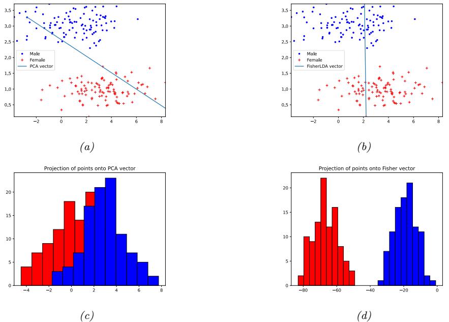
Figure 9.4: Linear disciminant analysis applied to two class dataset in 2d, representing (standardized) height and weight for male and female adults (a) PCA direction. (b) FLDA direction. (c) Projection onto PCA direction shows poor class separation. (d) Projection onto FLDA direction shows good class separation. Generated by fisher\_lda\_demo.ipynb.

9.2.6.1 Derivation of the optimal 1d projection

We now derive this optimal direction w, for the two-class case, following the presentation of [Bis06, Sec 4.1.4]. Define the class-conditional means as

\[\mu\_1 = \frac{1}{N\_1} \sum\_{n: y\_n = 1} x\_n, \ \mu\_2 = \frac{1}{N\_2} \sum\_{n: y\_n = 2} x\_n \tag{9.27}\]

Let m^k = w^Tµ^k be the projection of each mean onto the line w. Also, let zⁿ = w^Txⁿ be the projection of the data onto the line. The variance of the projected points is proportional to

\[s\_k^2 = \sum\_{n: y\_n = k} (z\_n - m\_k)^2 \tag{9.28}\]

The goal is to find w such that we maximize the distance between the means, m² ↑ m1, while also ensuring the projected clusters are “tight”, which we can do by minimizing their variance. This suggests the following objective:

\[J(\mathbf{w}) = \frac{(m\_2 - m\_1)^2}{s\_1^2 + s\_2^2} \tag{9.29}\]

We can rewrite the right hand side of the above in terms of w as follows

\[J(w) = \frac{w^{\mathsf{T}} \mathbf{S}\_B w}{w^{\mathsf{T}} \mathbf{S}\_W w} \tag{9.30}\]

where S^B is the between-class scatter matrix given by

\[\mathbf{S}\_B = (\mu\_2 - \mu\_1)(\mu\_2 - \mu\_1)^\mathsf{T} \tag{9.31}\]

and S^W is the within-class scatter matrix, given by

\[\mathbf{S}\_{W} = \sum\_{n: y\_{n} = 1} (x\_{n} - \mu\_{1})(x\_{n} - \mu\_{1})^{\mathsf{T}} + \sum\_{n: y\_{n} = 2} (x\_{n} - \mu\_{2})(x\_{n} - \mu\_{2})^{\mathsf{T}} \tag{9.32}\]

To see this, note that

\[\boldsymbol{w}^{\mathsf{T}} \mathbf{S}\_{B} \boldsymbol{w} = \boldsymbol{w}^{\mathsf{T}} (\boldsymbol{\mu}\_{2} - \boldsymbol{\mu}\_{1})(\boldsymbol{\mu}\_{2} - \boldsymbol{\mu}\_{1})^{\mathsf{T}} \boldsymbol{w} = (m\_{2} - m\_{1})(m\_{2} - m\_{1})\tag{9.33}\]

and

\[\begin{aligned} \boldsymbol{w}^{\mathsf{T}} \mathbf{S}\_{W} \boldsymbol{w} &= \sum\_{n: y\_{n} = 1} \boldsymbol{w}^{\mathsf{T}} (\boldsymbol{x}\_{n} - \boldsymbol{\mu}\_{1}) (\boldsymbol{x}\_{n} - \boldsymbol{\mu}\_{1})^{\mathsf{T}} \boldsymbol{w} + \\ &\sum\_{n: y\_{n} = 2} \boldsymbol{w}^{\mathsf{T}} (\boldsymbol{x}\_{n} - \boldsymbol{\mu}\_{2}) (\boldsymbol{x}\_{n} - \boldsymbol{\mu}\_{2})^{\mathsf{T}} \boldsymbol{w} \end{aligned} \tag{9.34}\]

\[=\sum\_{n:y\_n=1} \left(z\_n - m\_1\right)^2 + \sum\_{n:y\_n=2} \left(z\_n - m\_2\right)^2\tag{9.35}\]

Equation (9.30) is a ratio of two scalars; we can take its derivative with respect to w and equate to zero. One can show (Exercise 9.1) that J(w) is maximized when

\[\mathbf{S}\_B \mathbf{w} = \lambda \mathbf{S}\_W \mathbf{w} \tag{9.36}\]

where

\[\lambda = \frac{\boldsymbol{w}^{\mathsf{T}} \mathbf{S}\_{B} \boldsymbol{w}}{\boldsymbol{w}^{\mathsf{T}} \mathbf{S}\_{W} \boldsymbol{w}} \tag{9.37}\]

Equation (9.36) is called a generalized eigenvalue problem. If S^W is invertible, we can convert it to a regular eigenvalue problem:

\[\mathbf{S}\_W^{-1} \mathbf{S}\_B w = \lambda w\]

However, in the two class case, there is a simpler solution. In particular, since

\[\mathbf{S}\_B \mathbf{w} = (\mu\_2 - \mu\_1)(\mu\_2 - \mu\_1)^\mathsf{T} \mathbf{w} = (\mu\_2 - \mu\_1)(m\_2 - m\_1) \tag{9.39}\]

then, from Equation (9.38) we have

\[ \lambda \text{ } \mathbf{w} = \mathbf{S}\_W^{-1} (\mu\_2 - \mu\_1)(m\_2 - m\_1) \tag{9.40} \]

\[\mathbf{w} \propto \mathbf{S}\_W^{-1} (\mu\_2 - \mu\_1) \tag{9.41}\]

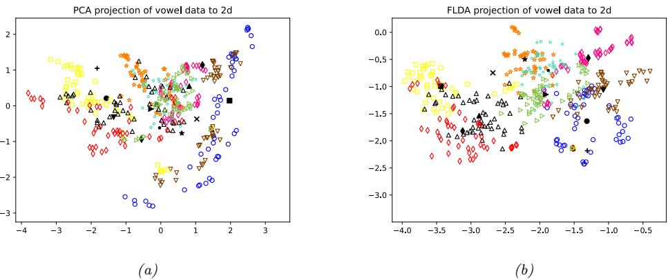
Figure 9.5: (a) PCA projection of vowel data to 2d. (b) FLDA projection of vowel data to 2d. We see there is better class separation in the FLDA case. Adapted from Figure 4.11 of [HTF09]. Generated by fisher\_discrim\_vowel.ipynb.

Since we only care about the directionality, and not the scale factor, we can just set

\[w = \mathbf{S}\_W^{-1} (\mu\_2 - \mu\_1) \tag{9.42}\]

This is the optimal solution in the two-class case. If S^W ∞ I, meaning the pooled covariance matrix is isotropic, then w is proportional to the vector that joins the class means. This is an intuitively reasonable direction to project onto, as shown in Figure 9.3.

9.2.6.2 Extension to higher dimensions and multiple classes

We can extend the above idea to multiple classes, and to higher dimensional subspaces, by finding a projection matrix W which maps from D to K. Let zⁿ = Wxⁿ be the low dimensional projection of the n’th data point. Let m^c = ¹ N^c $ ⁿ:yn=^c zⁿ be the corresponding mean for the c’th class and m = ¹ N $^{C c}=1 Ncm^c be the overall mean, both in the low dimensional space. We define the following scatter matrices:

\[\tilde{\mathbf{S}}\_{W} = \sum\_{c=1}^{C} \sum\_{n: y\_n = c} (\mathbf{z}\_n - \mathbf{m}\_c)(\mathbf{z}\_n - \mathbf{m}\_c)^\top \tag{9.43}\]

\[\bar{\mathbf{S}}\_B = \sum\_{c=1}^C N\_c (m\_c - m)(m\_c - m)^\top \tag{9.44}\]

Finally, we define the objective function as maximizing the following:2

\[J(\mathbf{W}) = \frac{|\tilde{\mathbf{S}}\_B|}{|\tilde{\mathbf{S}}\_W|} = \frac{|\mathbf{W}^\mathsf{T} \mathbf{S}\_B \mathbf{W}|}{|\mathbf{W}^\mathsf{T} \mathbf{S}\_W \mathbf{W}|} \tag{9.45}\]

2. An alternative criterion that is sometimes used [Fuk90] is ^J(W) = tr ! S˜→^{1 W S}˜^B ” = tr # (WSWWT)→1(WSBWT) $ .

where S^W and S^B are defined in the original high dimensional space in the obvious way (namely using xⁿ instead of zn, µ^c instead of mc, and µ instead of m). The solution can be shown [DHS01] to be ^{W = S→ 1} 2 ^{W U}, where ^U are the ^K leading eigenvectors of ^{S→ 1} 2 ^{W S}BS^{→ 1} 2 ^W , assuming S^W is non-singular. (If it is singular, we can first perform PCA on all the data.)

Figure 9.5 gives an example of this method applied to some D = 10 dimensional speech data, representing C = 11 di!erent vowel sounds. We project to K = 2 dimensions in order to visualize the data. We see that FLDA gives better class separation than PCA.

Note that FLDA is restricted to finding at most a K ↘ C ↑ 1 dimensional linear subspace, no matter how large D, because the rank of the between class scatter matrix S^B is C ↑ 1. (The -1 term arises because of the µ term, which is a linear function of the µc.) This is a rather severe restriction which limits the usefulness of FLDA.

9.3 Naive Bayes classifiers

In this section, we discuss a simple generative approach to classification in which we assume the features are conditionally independent given the class label. This is called the naive Bayes assumption. The model is called “naive” since we do not expect the features to be independent, even conditional on the class label. However, even if the naive Bayes assumption is not true, it often results in classifiers that work well [DP97; HY01a]. One reason for this is that the model is quite simple (it only has O(CD) parameters, for C classes and D features), and hence it is relatively immune to overfitting.

More precisely, the naive Bayes assumption corresponds to using a class conditional density of the following form:

\[p(\mathbf{z}|y=c,\boldsymbol{\theta}) = \prod\_{d=1}^{D} p(x\_d|y=c,\boldsymbol{\theta}\_{dc}) \tag{9.46}\]

where ωdc are the parameters for the class conditional density for class c and feature d. Hence the posterior over class labels is given by

\[p(y=c|\mathbf{z}, \boldsymbol{\theta}) = \frac{p(y=c|\boldsymbol{\pi}) \prod\_{d=1}^{D} p(x\_d|y=c, \boldsymbol{\theta}\_{dc})}{\sum\_{c'} p(y=c'|\boldsymbol{\pi}) \prod\_{d=1}^{D} p(x\_d|y=c', \boldsymbol{\theta}\_{dc'})} \tag{9.47}\]

where ϑ^c is the prior probability of class c, and ω = (ς, {ωdc}) are all the parameters. This is known as a naive Bayes classifier or NBC.

9.3.1 Example models

We still need to specify the form of the probability distributions in Equation (9.46). This depends on what type of feature x^d is. We give some examples below:

• In the case of binary features, x^d → {0, 1}, we can use the Bernoulli distribution: p(x|y = c, ω) = ^{D d}=1 Ber(xd|ϖdc), where ϖdc is the probability that x^d = 1 in class c. This is sometimes called the multivariate Bernoulli naive Bayes model. For example, Figure 9.6 shows the estimated parameters for each class when we fit this model to a binarized version of MNIST. This approach

Figure 9.6: Visualization of the Bernoulli class conditional densities for a naive Bayes classifier fit to a binarized version of the MNIST dataset. Generated by naive\_bayes\_mnist\_jax.ipynb.

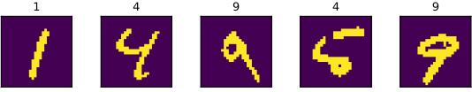
Figure 9.7: Visualization of the predictions made by the model in Figure 9.6 when applied to some binarized MNIST test images. The title shows the most probable predicted class. Generated by naive\_bayes\_mnist\_jax.ipynb.

does surprisingly well, and has a test set accuracy of 84.3%. (See Figure 9.7 for some sample predictions.)

• In the case of categorical features, x^d → {1,…,K}, we can use the categorical distribution: ^p(x|^{y =} c, ^ω) = ^{D d}=1 Cat(xd|ωdc), where ϖdck is the probability that x^d = k given that y = c.
• In the case of real-valued features, x^d → R, we can use the univariate Gaussian distribution: ^p(x|^{y =} c, ^ω) = ^{D d}=1 ^N (xd|µdc, ^ε2 dc), where µdc is the mean of feature d when the class label is c, and ε² dc is its variance. (This is equivalent to Gaussian discriminant analysis using diagonal covariance matrices.)

9.3.2 Model fitting

In this section, we discuss how to fit a naive Bayes classifier using maximum likelihood estimation. We can write the likelihood as follows:

\[p(\mathcal{D}|\boldsymbol{\theta}) = \prod\_{n=1}^{N} \left[ \text{Cat}(y\_n|\boldsymbol{\pi}) \prod\_{d=1}^{D} p(x\_{nd}|y\_n, \boldsymbol{\theta}\_d) \right] \tag{9.48}\]

\[=\prod\_{n=1}^{N} \left[ \text{Cat}(y\_n|\pi) \prod\_{d=1}^{D} \prod\_{c=1}^{C} p(x\_{nd}|\theta\_{dc})^{\mathbb{I}(y\_n=c)} \right] \tag{9.49}\]

so the log-likelihood is given by

\[\log p(\mathcal{D}|\boldsymbol{\theta}) = \left[ \sum\_{n=1}^{N} \sum\_{c=1}^{C} \mathbb{I} \left( y\_n = c \right) \log \pi\_c \right] + \sum\_{c=1}^{C} \sum\_{d=1}^{D} \left[ \sum\_{n: y\_n = c} \log p(x\_{nd}|\boldsymbol{\theta}\_{dc}) \right] \tag{9.50}\]

We see that this decomposes into a term for ς, and CD terms for each ωdc:

\[\log p(\mathcal{D}|\boldsymbol{\theta}) = \log p(\mathcal{D}\_y|\boldsymbol{\pi}) + \sum\_{c} \sum\_{d} \log p(\mathcal{D}\_{dc}|\boldsymbol{\theta}\_{dc}) \tag{9.51}\]

where D^y = {yⁿ : n =1: N} are all the labels, and Ddc = {xnd : yⁿ = c} are all the values of feature d for examples from class c. Hence we can estimate these parameters separately.

In Section 4.2.4, we show that the MLE for ς is the vector of empirical counts, ϑˆ^c = ^{Nc N} . The MLEs for ωdc depend on the choice of the class conditional density for feature d. We discuss some common choices below.

• In the case of discrete features, we can use a categorical distribution. A straightforward extension of the results in Section 4.2.4 gives the following expression for the MLE:

\[\hat{\theta}\_{dek} = \frac{N\_{dck}}{\sum\_{k'=1}^{K} N\_{dck'}} = \frac{N\_{dck}}{N\_c} \tag{9.52}\]

where Ndck = $^{N n}=1 I(xnd = k, yⁿ = c) is the number of times that feature d had value k in examples of class c.

• In the case of binary features, the categorical distribution becomes the Bernoulli, and the MLE becomes

\[\hat{\theta}\_{dc} = \frac{N\_{dc}}{N\_c} \tag{9.53}\]

which is the empirical fraction of times that feature d is on in examples of class c.

• In the case of real-valued features, we can use a Gaussian distribution. A straightforward extension of the results in Section 4.2.5 gives the following expression for the MLE:

\[ \hat{\mu}\_{dc} = \frac{1}{N\_c} \sum\_{n: y\_n = c} x\_{nd} \tag{9.54} \]

\[ \hat{\sigma}\_{dc}^2 = \frac{1}{N\_c} \sum\_{n: y\_n = c} (x\_{nd} - \hat{\mu}\_{dc})^2 \tag{9.55} \]

Thus we see that fitting a naive Bayes classifier is extremely simple and e”cient.

9.3.3 Bayesian naive Bayes

In this section, we extend our discussion of MLE estimation for naive Bayes classifiers from Section 9.3.2 to compute the posterior distribution over the parameters. For simplicity, let us assume we have categorical features, so p(xd|ωdc) = Cat(xd|ωdc), where ϖdck = p(x^d = k|y = c). In Section 4.6.3.2, we show that the conjugate prior for the categorical likelihood is the Dirichlet distribution, p(ωdc) = Dir(ωdc|εdc), where 1dck can be interpereted as a set of “pseudo counts”, corresponding to counts Ndck that come from prior data. Similarly we use a Dirichlet prior for the label frequencies, p(ς) = Dir(ς|φ). By using a conjugate prior, we can compute the posterior in closed form, as we explain in Section 4.6.3. In particular, we have

\[p(\boldsymbol{\theta}|\mathcal{D}) = \text{Dir}(\boldsymbol{\pi}|\boldsymbol{\hat{\alpha}}) \prod\_{d=1}^{D} \prod\_{c=1}^{C} \text{Dir}(\boldsymbol{\theta}\_{dc}|\boldsymbol{\hat{\beta}}\_{dc}) \tag{9.56}\]

where ↭ϱc=↫ϱ^{c +}N^c and ↭ ¹dck=↫ 1dck +Ndck.

Using the results from Section 4.6.3.4, we can derive the posterior predictive distribution as follows. For the label prior (before seeing x, but after seeing D), we have p(y|D) = Cat(y|ς), where ϑ^c =↭ϱ^c / $ c→ ↭ϱc^→ . For the feature likelihood of ^x (given ^y and ^D), we have ^p(x^{d = k}|^{y =} c, ^D) = ^ϖdck, where

\[\overline{\theta}\_{dck} = \frac{\overline{\beta}\_{dck}}{\sum\_{k'=1}^{K} \overline{\beta}\_{dck'}} = \frac{\overline{\beta}\_{dck} + N\_{dck}}{\sum\_{k'=1}^{K} \overline{\beta}\_{dck'} + N\_{dck'}}\tag{9.57}\]

is the posterior mean of the parameters. (Note that $^{K k}→=1 Ndck^→ = Ndc = N^c is the number of examples for class c.)

If ↫ ¹dck= 0, this reduces to the MLE in Equation (9.52). By contrast, if we set ↫ 1dck= 1, we add 1 to all the empirical counts before normalizing. This is called add-one smoothing or Laplace smoothing. For example, in the binary case, this gives

\[\overline{\theta}\_{dc} = \frac{\overset{\gtrless}{\beta}\_{dc1} + N\_{dc1}}{\overline{\beta}\_{dc0} + N\_{dc0} + \overline{\beta}\_{dc1} + N\_{dc1}} = \frac{1 + N\_{dc1}}{2 + N\_{dc}} \tag{9.58}\]

We can finally compute the posterior predictive distribution over the label as follows:

\[p(y=c|x, \mathcal{D}) \propto p(y=c|\mathcal{D}) \prod\_{d} p(x\_d|y=c, \mathcal{D}) = \overline{\pi}\_c \prod\_{d} \prod\_{k} \overline{\theta}\_{dck}^{\mathbb{I}(x\_d=k)} \tag{9.59}\]

This gives us a fully Bayesian form of naive Bayes, in which we have integrated out all the parameters. (In this case, the predictive distribution can be obtained merely by plugging in the posterior mean parameters.)

9.3.4 The connection between naive Bayes and logistic regression

In this section, we show that the class posterior p(y|x, ω) for a NBC model has the same form as multinomial logistic regression. For simplicity, we assume that the features are all discrete, and each has K states, although the result holds for arbitrary feature distributions in the exponential family.

Let xdk = I(x^d = k), so x^d is a one-hot encoding of feature d. Then the class conditional density can be written as follows:

\[p(\mathbf{z}|y=c,\boldsymbol{\theta}) = \prod\_{d=1}^{D} \text{Cat}(x\_d|y=c,\boldsymbol{\theta}) = \prod\_{d=1}^{D} \prod\_{k=1}^{K} \theta\_{dck}^{x\_{dk}} \tag{9.60}\]

Hence the posterior over classes is given by

\[p(y = c | \mathbf{z}, \boldsymbol{\theta}) = \frac{\pi\_c \prod\_d \prod\_k \theta\_{dck}^{x\_{dk}}}{\sum\_{c'} \pi\_{c'} \prod\_d \prod\_k \theta\_{dc'k}^{x\_{dk}}} = \frac{\exp[\log \pi\_c + \sum\_d \sum\_k x\_{dk} \log \theta\_{dck}]}{\sum\_{c'} \exp[\log \pi\_{c'} + \sum\_d \sum\_k x\_{dk} \log \theta\_{dc'k}]} \tag{9.61}\]

This can be written as a softmax

\[p(y=c|\mathbf{z}, \boldsymbol{\theta}) = \frac{e^{\boldsymbol{\theta}^{\mathsf{T}}\boldsymbol{\mathsf{z}} + \gamma\_c}}{\sum\_{c'=1}^{C} e^{\boldsymbol{\theta}^{\mathsf{T}}\_{c'}\boldsymbol{\mathsf{z}} + \gamma\_{c'}}}\tag{9.62}\]

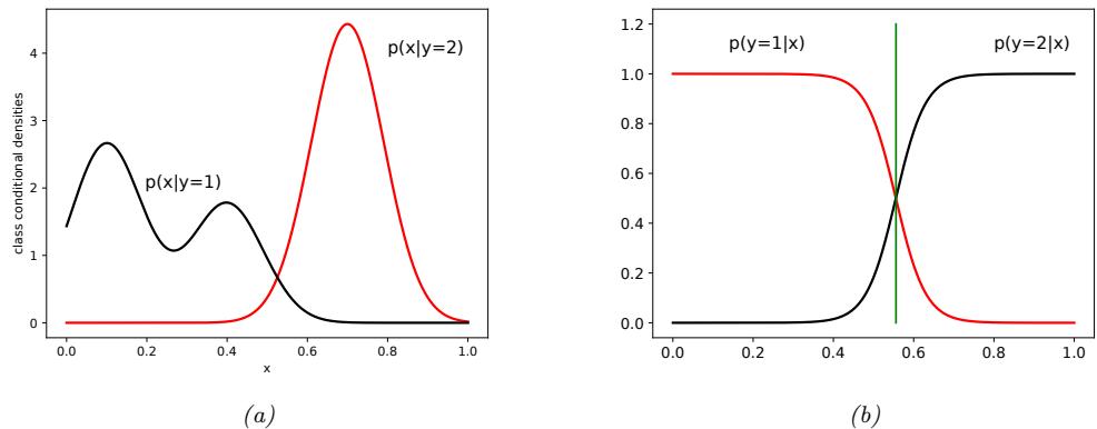
Figure 9.8: The class-conditional densities p(x|y = c) (left) may be more complex than the class posteriors p(y = c|x) (right). Adapted from Figure 1.27 of [Bis06]. Generated by generativeVsDiscrim.ipynb.

by suitably defining ε^c and ⇁c. This has exactly the same form as multinomial logistic regression in Section 2.5.3. The di!erence is that with naive Bayes we optimize the joint likelihood ⁿ p(yn, xn|ω), whereas with logistic regression, we optimize the conditional likelihood ⁿ p(yn|xn, ω). In general, these can give di!erent results (see Exercise 10.3).

9.4 Generative vs discriminative classifiers

A model of the form p(x, y) = p(y)p(x|y) is called a generative classifier, since it can be used to generate examples x from each class y. By contrast, a model of the form p(y|x) is called a discriminative classifier, since it can only be used to discriminate between di!erent classes. Below we discuss various pros and cons of the generative and discriminative approaches to classification. (See also [BT04; UB05; LBM06; BL07a; Rot+18].)

9.4.1 Advantages of discriminative classifiers

The main advantages of discriminative classifiers are as follows:

• Better predictive accuracy. Discriminative classifiers are often much more accurate than generative classifiers [NJ02]. The reason is that the conditional distribution p(y|x) is often much simpler (and therefore easier to learn) than the joint distribution p(y, x), as illustrated in Figure 9.8. In particular, discriminative models do not need to “waste e!ort” modeling the distribution of the input features.
• Can handle feature preprocessing. A big advantage of discriminative methods is that they allow us to preprocess the input in arbitrary ways. For example, we can perform a polynomial expansion of the input features, and we can replace a string of words with embedding vectors (see Section 20.5). It is often hard to define a generative model on such pre-processed data, since the new features can be correlated in complex ways which are hard to model.

• Well-calibrated probabilities. Some generative classifiers, such as naive Bayes (described in Section 9.3), make strong independence assumptions which are often not valid. This can result in very extreme posterior class probabilities (very near 0 or 1). Discriminative models, such as logistic regression, are often better calibrated in terms of their probability estimates, although they also sometimes need adjustment (see e.g., [NMC05]).

9.4.2 Advantages of generative classifiers

The main advantages of generative classifiers are as follows:

• Easy to fit. Generative classifiers are often very easy to fit. For example, in Section 9.3.2, we show how to fit a naive Bayes classifier by simple counting and averaging. By contrast, logistic regression requires solving a convex optimization problem (see Section 10.2.3 for the details), and neural nets require solving a non-convex optimization problem, both of which are much slower.
• Can easily handle missing input features. Sometimes some of the inputs (components of x) are not observed. In a generative classifier, there is a simple method for dealing with this, as we show in Section 1.5.5. However, in a discriminative classifier, there is no principled solution to this problem, since the model assumes that x is always available to be conditioned on.
• Can fit classes separately. In a generative classifier, we estimate the parameters of each class conditional density independently (as we show in Section 9.3.2), so we do not have to retrain the model when we add more classes. In contrast, in discriminative models, all the parameters interact, so the whole model must be retrained if we add a new class.
• Can handle unlabeled training data. It is easy to use generative models for semi-supervised learning, in which we combine labeled data Dxy = {(xn, yn)} and unlabeled data, D^x = {xn}. However, this is harder to do with discriminative models, since there is no uniquely optimal way to exploit Dx.
• May be more robust to spurious features. A discriminative model p(y|x) may pick up on features of the input x that can discriminate di!erent values of y in the training set, but which are not robust and do not generalize beyond the training set. These are called spurious features (see e.g., [Arj21; Zho+21]). By contrast, a generative model p(x|y) may be better able to capture the causal mechanisms of the underlying data generating process; such causal models can be more robust to distribution shift (see e.g., [Sch19; LBS19; LN81]).

9.4.3 Handling missing features

Sometimes we are missing parts of the input x during training and/or testing. In a generative classifier, we can handle this situation by marginalizing out the missing values. (We assume that the missingness of a feature is not informative about its potential value.) By contrast, when using a discriminative model, there is no unique best way to handle missing inputs, as we discuss in Section 1.5.5.

For example, suppose we are missing the value of x1. We just have to compute

\[p(y = c | \mathbf{x}\_{2:D}, \boldsymbol{\theta}) \propto p(y = c | \boldsymbol{\pi}) p(\mathbf{x}\_{2:D} | y = c, \boldsymbol{\theta}) \tag{9.63}\]

\[=p(y=c|\pi)\sum\_{x\_1}p(x\_1,x\_{2:D}|y=c,\boldsymbol{\theta})\tag{9.64}\]

In Gaussian discriminant analysis, we can marginalize out x¹ using the equations from Section 3.2.3.

If we make the naive Bayes assumption, things are even easier, since we can just ignore the likelihood term for x1. This follows because

\[\sum\_{x\_1} p(x\_1, x\_{2:D} | y = c, \boldsymbol{\theta}) = \left[ \sum\_{x\_1} p(x\_1 | \boldsymbol{\theta}\_{1c}) \right] \prod\_{d=2}^{D} p(x\_d | \boldsymbol{\theta}\_{dc}) = \prod\_{d=2}^{D} p(x\_d | \boldsymbol{\theta}\_{dc}) \tag{9.65}\]

where we exploited the fact that ^p(xd|^{y =} c, ^ω) = ^p(xd|ωdc) and $ ^x1 p(x1|ω1c)=1.

9.5 Exercises

Exercise 9.1 [Derivation of Fisher’s linear discriminant]

Show that the maximum of J(w) = ^{wT S}B^{w wT SW w} is given by SBw = ↼S^W w where ↼ = ^{wT S}B^{w wT SW w} . Hint: recall that the derivative of a ratio of two scalars is given by ^d dx f(x) ^g(x) ^{= f}→g→fg^{→ g2} , where f^↓ = ^d dx f(x) and g^↓ = ^d dx g(x). Also, recall that ^{d dx xT Ax} = (^{A + AT} )x.

10 Logistic Regression

10.1 Introduction

Logistic regression is a widely used discriminative classification model ^p(y|x; ^ω), where ^{x → RD} is a fixed-dimensional input vector, y → {1,…,C} is the class label, and ω are the parameters. If C = 2, this is known as binary logistic regression, and if C > 2, it is known as multinomial logistic regression, or alternatively, multiclass logistic regression. We give the details below.

10.2 Binary logistic regression

Binary logistic regression corresponds to the following model

\[p(y|\mathbf{x}, \theta) = \text{Ber}(y|\sigma(\mathbf{w}^\mathsf{T}\mathbf{x} + b))\tag{10.1}\]

where ε is the sigmoid function defined in Section 2.4.2, w are the weights, b is the bias, and ω = (w, b) are all the parameters. In other words,

\[p(y=1|x,\theta) = \sigma(a) = \frac{1}{1+e^{-a}}\tag{10.2}\]

where a = w^Tx + b = log( ^{p 1}→^p ), is the log-odds, and ^{p = p}(^y = 1|x, ^ω). (In ML, the quantity ^a is usually called the logit or the pre-activation.)

Sometimes we choose to use the labels y˜ → {↑1, +1} instead of y → {0, 1}. We can compute the probability of these alternative labels using

\[p(\ddot{y}|\mathbf{x}, \theta) = \sigma(\ddot{y}a) \tag{10.3}\]

since ε(↑a)=1 ↑ ε(a). This slightly more compact notation is widely used in the ML literature.

10.2.1 Linear classifiers

The sigmoid gives the probability that the class label is y = 1. If the loss for misclassifying each class is the same, then the optimal decision rule is to predict y = 1 i! class 1 is more likely than class 0, as we explained in Section 5.1.2.2. Thus

\[f(\mathbf{x}) = \mathbb{I}\left(p(y=1|\mathbf{x}) > p(y=0|\mathbf{x})\right) = \mathbb{I}\left(\log \frac{p(y=1|\mathbf{x})}{p(y=0|\mathbf{x})} > 0\right) = \mathbb{I}\left(a > 0\right) \tag{10.4}\]

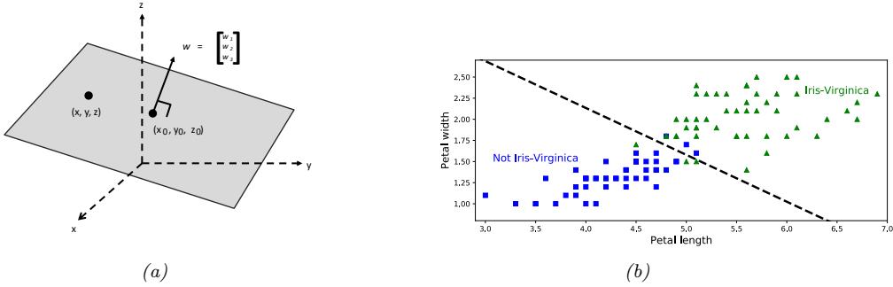
Figure 10.1: (a) Visualization of a 2d plane in a 3d space with surface normal w going through point x⁰ = (x0, y0, z0). See text for details. (b) Visualization of optimal linear decision boundary induced by logistic regression on a 2-class, 2-feature version of the iris dataset. Generated by iris\_logreg.ipynb. Adapted from Figure 4.24 of [Gér19].

where a = w^Tx + b.

Thus we can write the prediction function as follows:

\[f(x; \theta) = b + w^{\top}x = b + \sum\_{d=1}^{D} w\_d x\_d \tag{10.5}\]

where ^wTx = ^∅w, ^xℜ is the inner product between the weight vector ^w and the feature vector ^x. This function defines a linear hyperplane, with normal vector ^{w → RD} and an o!set ^{b → R} from the origin.

Equation (10.5) can be understood by looking at Figure 10.1a. Here we show a plane in a 3d feature space going through the point x⁰ with surface normal w. Points on the surface satisfy ^wT(^{x ↑ x}0)=0. If we define ^{b = ↑}w^Tx0, we can rewrite this as ^{wTx + b} = 0. This plane separates 3d space into two half spaces. This linear plane is known as a decision boundary. If we can perfectly separate the training examples by such a linear boundary (without making any classification errors on the training set), we say the data is linearly separable. From Figure 10.1b, we see that the two-class, two-feature version of the iris dataset is not linearly separable.

In general, there will be uncertainty about the correct class label, so we need to predict a probability distribution over labels, and not just decide which side of the decision boundary we are on. In Figure 10.2, we plot p(y = 1|(x1, x2), w) = ε(w1x¹ +w2x2) for di!erent weight vectors w. The vector w defines the orientation of the decision boundary, and its magnitude, ||w|| = G$^{D d}=1 w^{2 d}, controls the steepness of the sigmoid, and hence the confidence of the predictions.

10.2.2 Nonlinear classifiers

We can often make a problem linearly separable by preprocessing the inputs in a suitable way. In particular, let ϑ(x) be a transformed version of the input feature vector. For example, suppose we use ϑ(x1, x2) = [1, x² 1, x^{2 2}], and we let ^w = [↑R², ¹, 1]. Then ^wTϑ(x) = ^{x2 1} + x^{2 2 ↑ R2}, so the decision boundary (where f(x)=0) defines a circle with radius R, as shown in Figure 10.3. The resulting

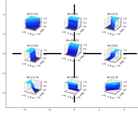
Figure 10.2: Plots of ϑ(w1x¹ +w2x2). Here w = (w1, w2) defines the normal to the decision boundary. Points to the right of this have ϑ(w^Tx) > 0.5, and points to the left have ϑ(w^Tx) < 0.5. Adapted from Figure 39.3 of [Mac03]. Generated by sigmoid\_2d\_plot.ipynb.

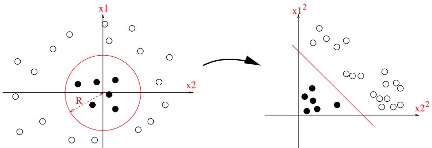
Figure 10.3: Illustration of how we can transform a quadratic decision boundary into a linear one by transforming the features from x = (x1, x2) to ϑ(x)=(x² 1, x^{2 2}). Used with kind permission of Jean-Philippe Vert.

function f is still linear in the parameters w, which is important for simplifying the learning problem, as we will see in Section 10.2.3. However, we can gain even more power by learning the parameters of the feature extractor ϑ(x) in addition to linear weights w; we discuss how to do this in Part III.

In Figure 10.3, we used a quadratic expansion of the features. We can also use a higher order polynomial, as in Section 1.2.2.2. In Figure 10.4, we show the e!ects of using polynomial expansion up to degree K on a 2d logistic regression problem. As in Figure 1.7, we see that the model becomes more complex as the number of parameters increases, and eventually results in overfitting. We discuss ways to reduce overfitting in Section 10.2.7.

10.2.3 Maximum likelihood estimation

In this section, we discuss how to estimate the parameters of a logistic regression model using maximum likelihood estimation.

10.2.3.1 Objective function

The negative log likelihood (scaled by the dataset size N) is given by the following (we assume the bias term b is absorbed into the weight vector w):

\[\text{NLL}(\boldsymbol{w}) = -\frac{1}{N} \log p(\mathcal{D}|\boldsymbol{w}) = -\frac{1}{N} \log \prod\_{n=1}^{N} \text{Ber}(y\_n|\mu\_n) \tag{10.6}\]

\[= -\frac{1}{N} \sum\_{n=1}^{N} \log[\mu\_n^{y\_n} \times (1 - \mu\_n)^{1 - y\_n}] \tag{10.7}\]

\[=-\frac{1}{N} \sum\_{n=1}^{N} \left[ y\_n \log \mu\_n + (1 - y\_n) \log(1 - \mu\_n) \right] \tag{10.8}\]

\[\mathcal{L} = \frac{1}{N} \sum\_{n=1}^{N} \mathbb{H}\_{ce}(y\_n, \mu\_n) \tag{10.9}\]

where µⁿ = ε(an) is the probability of class 1, aⁿ = w^Txⁿ is the logit, and Hce(yn, µn) is the binary cross entropy defined by

\[\mathbb{H}\_{ce}(p,q) = -\left[p\log q + (1-p)\log(1-q)\right] \tag{10.10}\]

If we use y˜ⁿ → {↑1, +1} instead of yⁿ → {0, 1}, then we can rewrite this as follows:

\[\text{NLL}(w) = -\frac{1}{N} \sum\_{n=1}^{N} \left[ \mathbb{I} \left( \check{y}\_n = 1 \right) \log(\sigma(a\_n)) + \mathbb{I} \left( \check{y}\_n = -1 \right) \log(\sigma(-a\_n)) \right] \tag{10.11}\]

\[\hat{y} = -\frac{1}{N} \sum\_{n=1}^{N} \log(\sigma(\tilde{y}\_n a\_n)) \tag{10.12}\]

\[=\frac{1}{N}\sum\_{n=1}^{N}\log(1+\exp(-\tilde{y}\_na\_n))\tag{10.13}\]

However, in this book, we will mostly use the yⁿ → {0, 1} notation, since it is easier to generalize to the multiclass case (Section 10.3), and makes the connection with cross-entropy easier to see.

10.2.3.2 Optimizing the objective

To find the MLE, we must solve

\[\nabla\_{\mathbf{w}} \text{NLL}(\mathbf{w}) = \mathbf{g}(\mathbf{w}) = \mathbf{0} \tag{10.14}\]

We can use any gradient-based optimization algorithm to solve this, such as those we discuss in Chapter 8. We give a specific example in Section 10.2.4. But first we must derive the gradient, as we explain below.

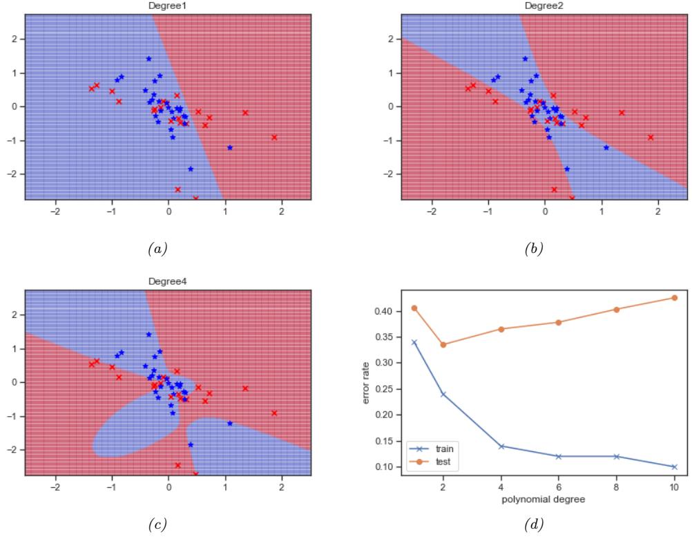
Figure 10.4: Polynomial feature expansion applied to a two-class, two-dimensional logistic regression problem. (a) Degree K = 1. (b) Degree K = 2. (c) Degree K = 4. (d) Train and test error vs degree. Generated by logreg\_poly\_demo.ipynb.

10.2.3.3 Deriving the gradient

Although we can use automatic di!erentiation methods (Section 13.3) to compute the gradient of the NLL, it is also easy to do explicitly, as we show below. Fortunately the resulting equations will turn out to have a simple and intuitive interpretation, which can be used to derive other methods, as we will see.

To start, note that

\[\frac{d\mu\_n}{da\_n} = \sigma(a\_n)(1 - \sigma(a\_n))\tag{10.15}\]

where aⁿ = w^Txⁿ and µⁿ = ε(an). Hence by the chain rule (and the rules of vector calculus, discussed in Section 7.8) we have

\[\frac{\partial}{\partial w\_d} \mu\_n = \frac{\partial}{\partial w\_d} \sigma(\mathbf{w}^\mathsf{T} \mathbf{z}\_n) = \frac{\partial}{\partial a\_n} \sigma(a\_n) \frac{\partial a\_n}{\partial w\_d} = \mu\_n (1 - \mu\_n) x\_{nd} \tag{10.16}\]

The gradient for the bias term can be derived in the same way, by using the input xn⁰ = 1 in the above equation. However, we will ignore the bias term for simplicity. Hence

\[ \nabla\_{\mathbf{w}} \log(\mu\_n) = \frac{1}{\mu\_n} \nabla\_{\mathbf{w}} \mu\_n = (1 - \mu\_n) \mathbf{x}\_n \tag{10.17} \]

Similarly,

\[\nabla\_{\mathbf{w}} \log(1 - \mu\_n) = \frac{-\mu\_n (1 - \mu\_n) x\_n}{1 - \mu\_n} = -\mu\_n x\_n \tag{10.18}\]

Thus the gradient vector of the NLL is given by

\[\nabla\_{\mathbf{w}} \text{NLL}(\mathbf{w}) = -\frac{1}{N} \sum\_{n=1}^{N} \left[ y\_n (1 - \mu\_n) x\_n - (1 - y\_n) \mu\_n x\_n \right] \tag{10.19}\]

\[=-\frac{1}{N}\sum\_{n=1}^{N}\left[y\_n\mathbf{z}\_n - y\_n\mathbf{z}\_n\boldsymbol{\mu}\_n - \mathbf{z}\_n\boldsymbol{\mu}\_n + y\_n\mathbf{z}\_n\boldsymbol{\mu}\_n\right] \tag{10.20}\]

\[\mathbf{x} = \frac{1}{N} \sum\_{n=1}^{N} (\mu\_n - y\_n) \mathbf{x}\_n \tag{10.21}\]

If we interpret eⁿ = µⁿ ↑ yⁿ as an error signal, we can see that the gradient weights each input xⁿ by its error, and then averages the result. Note that we can rewrite the gradient in matrix form as follows:

\[\nabla\_{\mathbf{w}} \text{NLL}(\mathbf{w}) = \frac{1}{N} (\mathbf{1}\_N^{\mathsf{T}} (\text{diag}(\boldsymbol{\mu} - \boldsymbol{y}) \mathbf{X}))^{\mathsf{T}} \tag{10.22}\]

where X is the N ↓ D design matrix containing the examples xⁿ in each row.

10.2.3.4 Deriving the Hessian

Gradient-based optimizers will find a stationary point where g(w) = 0. This could either be a global optimum or a local optimum. To be sure the stationary point is the global optimum, we must show that the objective is convex, for reasons we explain in Section 8.1.1.1. Intuitvely this means that the NLL has a bowl shape, with a unique lowest point, which is indeed the case, as illustrated in Figure 10.5b.

More formally, we must prove that the Hessian is positive semi-definite, which we now do. (See Chapter 7 for relevant background information on linear algebra.) One can show that the Hessian is given by

\[\mathbf{H}(\mathbf{w}) = \nabla\_{\mathbf{w}} \nabla\_{\mathbf{w}}^{\mathsf{T}} \text{NLL}(\mathbf{w}) = \frac{1}{N} \sum\_{n=1}^{N} (\mu\_n (1 - \mu\_n) x\_n) x\_n^{\mathsf{T}} = \frac{1}{N} \mathbf{X}^{\mathsf{T}} \mathbf{S} \mathbf{X} \tag{10.23}\]

where

\[\mathbf{S} \triangleq \text{diag}(\mu\_1 (1 - \mu\_1), \dots, \mu\_N (1 - \mu\_N)) \tag{10.24}\]

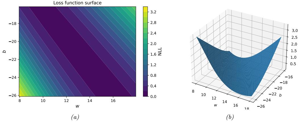
Figure 10.5: NLL loss surface for binary logistic regression applied to Iris dataset with 1 feature and 1 bias term. The goal is to minimize the function. The global MLE is at the center of the plot. Generated by iris\_logreg\_loss\_surface.ipynb.

We see that H is positive definite, since for any nonzero vector v, we have

\[v^{\mathsf{T}}\mathbf{X}^{\mathsf{T}}\mathbf{S}\mathbf{X}v = (v^{\mathsf{T}}\mathbf{X}^{\mathsf{T}}\mathbf{S}^{\frac{1}{2}})(\mathbf{S}^{\frac{1}{2}}\mathbf{X}v) = ||v^{\mathsf{T}}\mathbf{X}^{\mathsf{T}}\mathbf{S}^{\frac{1}{2}}||\_{2}^{2} > 0\tag{10.25}\]

This follows since µⁿ > 0 for all n, because of the use of the sigmoid function. Consequently the NLL is strictly convex. However, in practice, values of µⁿ which are close to 0 or 1 might cause the Hessian to be close to singular. We can avoid this by using ω² regularization, as we discuss in Section 10.2.7.

10.2.4 Stochastic gradient descent

Our goal is to solve the following optimization problem

\[ \hat{w} \stackrel{\Delta}{=} \operatorname\*{argmin}\_{w} \mathcal{L}(w) \tag{10.26} \]

where L(w) is the loss function, in this case the negative log likelihood:

\[\text{NLL}(w) = -\frac{1}{N} \sum\_{n=1}^{N} \left[ y\_n \log \mu\_n + (1 - y\_n) \log(1 - \mu\_n) \right] \tag{10.27}\]

where µⁿ = ε(an) is the probability of class 1, and aⁿ = w^Txⁿ is the log odds.

There are many algorithms we could use to solve Equation (10.26), as we discuss in Chapter 8. Perhaps the simplest is to use stochastic gradient descent (Section 8.4). If we use a minibatch of size 1, then we get the following simple update equation:

\[w\_{t+1} = w\_t - \eta\_t \nabla\_\mathbf{w} \text{NLL}(w\_t) = w\_t - \eta\_t (\mu\_n - y\_n) x\_n \tag{10.28}\]

where we replaced the average over all N examples in the gradient of Equation (10.21) with a single stochastically chosen sample n. (The index n changes with t.)

Since we know the objective is convex (see Section 10.2.3.4), then one can show that this procedure will converge to the global optimum, provided we decay the learning rate at the appropriate rate (see Section 8.4.3). We can improve the convergence speed using variance reduction techniques such as SAGA (Section 8.4.5.2).

10.2.5 Perceptron algorithm

A perceptron, first introduced in [Ros58], is a deterministic binary classifier of the following form:

\[f(\mathbf{z}\_n; \theta) = \mathbb{I}\left(\mathbf{w}^\mathsf{T} \mathbf{z}\_n + b > 0\right) \tag{10.29}\]

This can be seen to be a limiting case of a binary logistic regression classifier, in which the sigmoid function ε(a) is replaced by the Heaviside step function H(a) ↭ I(a > 0). See Figure 2.10 for a comparison of these two functions.

Since the Heaviside function is not di!erentiable, we cannot use gradient-based optimization methods to fit this model. However, Rosenblatt proposed the perceptron learning algorithm instead. The basic idea is to start with random weights, and then iteratively update them whenever the model makes a prediction mistake. More precisely, we update the weights using

\[\mathbf{w}\_{t+1} = \mathbf{w}\_t - \eta\_t (\hat{y}\_n - y\_n) \mathbf{z}\_n \tag{10.30}\]

where (xn, yn) is the labeled example sampled at iteration t, and ◁^t is the learning rate or step size. (We can set the step size to 1, since the magnitude of the weights does not a!ect the decision boundary.) See perceptron\_demo\_2d.ipynb for a simple implementation of this algorithm.

The perceptron update rule in Equation (10.30) has an intuitive interpretation: if the prediction is correct, no change is made, otherwise we move the weights in a direction so as to make the correct answer more likely. More precisely, if yⁿ = 1 and yˆⁿ = 0, we have wt+1 = w^t + xn, and if yⁿ = 0 and yˆⁿ = 1, we have wt+1 = w^t ↑ xn.

By comparing Equation (10.30) to Equation (10.28), we see that the perceptron update rule is equivalent to the SGD update rule for binary logistic regression using the approximation where we replace the soft probabilities µⁿ = p(yⁿ = 1|xn) with hard labels yˆⁿ = f(xn). The advantage of the perceptron method is that we don’t need to compute probabilities, which can be useful when the label space is very large. The disadvantage is that the method will only converge when the data is linearly separable [Nov62], whereas SGD for minimizing the NLL for logistic regression will always converge to the globally optimal MLE, even if the data is not linearly separable.

In Section 13.2, we will generalize perceptrons to nonlinear functions, thus significantly enhancing their usefulness.

10.2.6 Iteratively reweighted least squares

Gradient descent is a first order optimization method, which means it only uses first order gradients to navigate through the loss landscape. This can be slow, especially when some directions of space point steeply downhill, whereas other have a shallower gradient, as is the case in Figure 10.5a. In such problems, it can be much faster to use a second order optimization method, that takes the curvature of the space into account.

We discuss such methods in more detail in Section 8.3. Here we just consider a simple second order method that works well for logistic regression. We focus on the full batch setting (so we assume N is small), since it is harder to make second order methods work in the stochastic setting (see e.g., [Byr+16; Liu+18b] for some methods).

The classic second-order method is Newton’s method. This consists of updates of the form

\[w\_{t+1} = w\_t - \eta\_t \mathbf{H}\_t^{-1} g\_t \tag{10.31}\]

where

\[\mathbf{H}\_t \triangleq \nabla^2 \mathcal{L}(\boldsymbol{w})|\_{\mathbf{w}\_t} = \nabla^2 \mathcal{L}(\boldsymbol{w}\_t) = \mathbf{H}(\boldsymbol{w}\_t) \tag{10.32}\]

is assumed to be positive-definite to ensure the update is well-defined. If the Hessian is exact, we can set the step size to ◁^t = 1.

We now apply this method to logistic regression. Recall from Section 10.2.3.3 that the gradient and Hessian are given by

\[\nabla\_{\mathbf{w}} \text{NLL}(\mathbf{w}) = \frac{1}{N} \sum\_{n=1}^{N} (\mu\_n - y\_n) \mathbf{z}\_n \tag{10.33}\]

\[\mathbf{H} = \frac{1}{N} \mathbf{X}^{\mathsf{T}} \mathbf{S} \mathbf{X} \tag{10.34}\]

\[\mathbf{S} \triangleq \text{diag}(\mu\_1 (1 - \mu\_1), \dots, \mu\_N (1 - \mu\_N)) \tag{10.35}\]

Hence the Newton update has the form

\[w\_{t+1} = w\_t - \mathbf{H}^{-1} g\_t \tag{10.36}\]

\[=w\_t + (\mathbf{X}^\mathsf{T} \mathbf{S}\_t \mathbf{X})^{-1} \mathbf{X}^\mathsf{T} (y - \mu\_t) \tag{10.37}\]

\[\mathbf{x} = (\mathbf{X}^{\mathsf{T}} \mathbf{S}\_{l} \mathbf{X})^{-1} \left[ (\mathbf{X}^{\mathsf{T}} \mathbf{S}\_{l} \mathbf{X}) w\_{l} + \mathbf{X}^{\mathsf{T}} (y - \mu\_{t}) \right] \tag{10.38}\]

\[\mathbf{x} = (\mathbf{X}^{\mathsf{T}} \mathbf{S}\_{t} \mathbf{X})^{-1} \mathbf{X}^{\mathsf{T}} \left[ \mathbf{S}\_{t} \mathbf{X} w\_{t} + \boldsymbol{y} - \boldsymbol{\mu}\_{t} \right] \tag{10.39}\]

\[\mathbf{x} = (\mathbf{X}^{\mathsf{T}} \mathbf{S}\_{t} \mathbf{X})^{-1} \mathbf{X}^{\mathsf{T}} \mathbf{S}\_{t} z\_{t} \tag{10.40}\]

where we have defined the working response as

\[\mathbf{z}\_t \triangleq \mathbf{X}w\_t + \mathbf{S}\_t^{-1}(y - \mu\_t) \tag{10.41}\]

and S^t = diag(µt,n(1 ↑ µt,n)). Since S^t is a diagonal matrix, we can rewrite the targets in component form as follows:

\[z\_{t,n} = w\_t^\mathrm{T} x\_n + \frac{y\_n - \mu\_{t,n}}{\mu\_{t,n} (1 - \mu\_{t,n})} \tag{10.42}\]

Equation (10.40) is an example of a weighted least squares problem (Section 11.2.2.4), which is a minimizer of

\[\sum\_{n=1}^{N} S\_{t,n} (z\_{t,n} - w\_t^\top x\_n)^2 \tag{10.43}\]

Algorithm 10.1: Iteratively reweighted least squares (IRLS)

1 w = 0
2 repeat
3	for n =1: N do
4	wTxn an =
5	µn = ε(an)
6	sn = µn(1 ↑ µn)
7	yn→µn zn = an + sn
8	S = diag(s1:N )
9	(XTSX)→1XTSz w =
	10 until converged

The overall method is therefore known as the iteratively reweighted least squares (IRLS) algorithm, since at each iteration we solve a weighted least squares problem, where the weight matrix S^t changes at each iteration. See Algorithm 10.1 for some pseudocode.

Note that Fisher scoring is the same as IRLS except we replace the Hessian of the actual log-likelihood with its expectation, i.e., we use the Fisher information matrix (Section 4.7.2) instead of H. Since the Fisher information matrix is independent of the data, it can be precomputed, unlike the Hessian, which must be reevaluated at every iteration. This can be faster for problems with many parameters.

10.2.7 MAP estimation

In Figure 10.4, we saw how logistic regression can overfit when there are too many parameters compared to training examples. This is a consequence of the ability of maximum likelihood to find weights that force the decision boundary to “wiggle” in just the right way so as to curve around the examples. To get this behavior, the weights often need to be set to large values. For example, in Figure 10.4, when we use degree K = 1, we find that the MLE for the two input weights (ignoring the bias) is

wˆ = [0.51291712, 0.11866937] (10.44)

When we use degree K = 2, we get

\[ \hat{\mathbf{w}} = [2.27510513, 0.05970325, 11.84198867, 15.40355969, 2.51242311] \tag{10.45} \]

And when K = 4, we get

\[ \hat{\mathbf{w}} = [-3.07813766, \cdots, -59.03196044, 51.77152431, 10.25054164] \tag{10.46} \]

One way to reduce such overfitting is to prevent the weights from becoming so large. We can do this by using a zero-mean Gaussian prior, p(w) = N (w|0, CI), and then using MAP estimation, as we discussed in Section 4.5.3. The new training objective becomes

\[\mathcal{L}(\mathbf{w}) = \text{NLL}(\mathbf{w}) + \lambda ||\mathbf{w}||\_2^2 \tag{10.47}\]

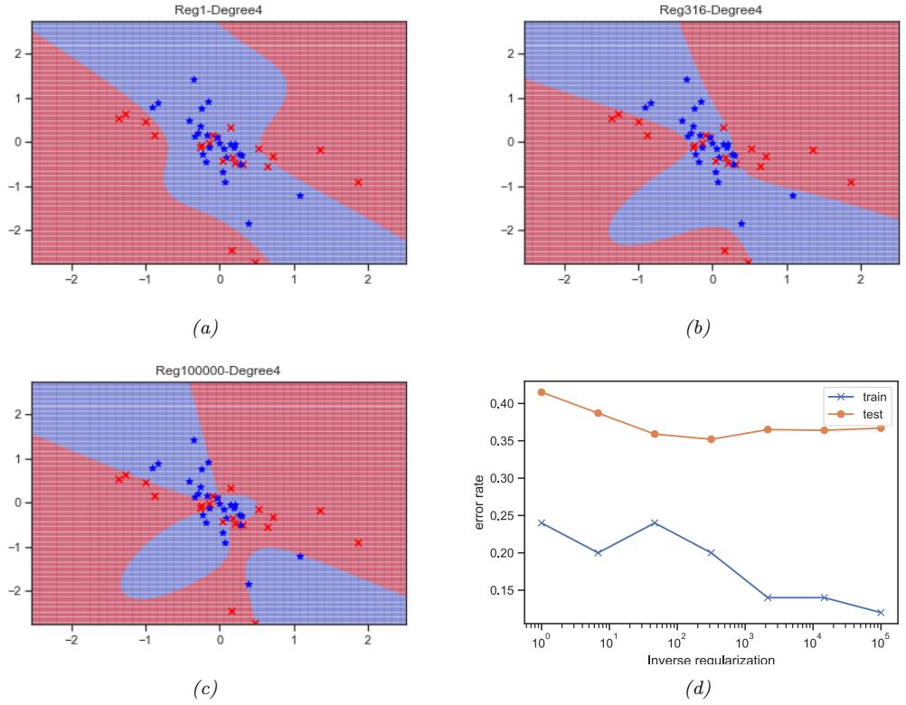
Figure 10.6: Weight decay with variance C applied to two-class, two-dimensional logistic regression problem with a degree 4 polynomial. (a) C = 1. (b) C = 316. (c) C = 100, 000. (d) Train and test error vs C. Generated by logreg\_poly\_demo.ipynb.

where ||w||^{2 2} = $^{D d}=1 w^{2 d} and φ = 1/C. This is called ω² regularization or weight decay. The larger the value of φ, the more the parameters are penalized for being “large” (deviating from the zero-mean prior), and thus the less flexible the model. See Figure 10.6 for an illustration.

We can compute the MAP estimate by slightly modifying the input to the above gradient-based optimization algorithms. The gradient and Hessian of the penalized negative log likelihood have the following forms:

\[\text{PNLL}(w) = \text{NLL}(w) + \lambda w^{\text{T}} w \tag{10.48}\]

\[\nabla\_{\mathbf{w}} \text{PNLL}(w) = \mathbf{g}(w) + 2\lambda w \tag{10.49}\]

\[\nabla\_{\mathbf{w}}^{2} \text{PNLL}(\mathbf{w}) = \mathbf{H}(\mathbf{w}) + 2\lambda \mathbf{I} \tag{10.50}\]

where g(w) is the gradient and H(w) is the Hessian of the unpenalized NLL.

For an interesting exercise related to ω² regularized logistic regression, see Exercise 10.2.

10.2.8 Standardization

In Section 10.2.7, we use an isotropic prior ^N (w|0, ^φ→¹I) to prevent overfitting. This implicitly encodes the assumption that we expect all weights to be similar in magnitude, which in turn encodes the assumption we expect all input features to be similar in magnitude. However, in many datasets, input features are on di!erent scales. In such cases, it is common to standardize the data, to ensure each feature has mean 0 and variance 1. We can do this by subtracting the mean and dividing by the standard deviation of each feature, as follows:

\[\text{standardize}(x\_{nd}) = \frac{x\_{nd} - \hat{\mu}\_d}{\hat{\sigma}\_d} \tag{10.51}\]

\[ \hat{\mu}\_d = \frac{1}{N} \sum\_{n=1}^{N} x\_{nd} \tag{10.52} \]

\[ \hat{\sigma}\_d^2 = \frac{1}{N} \sum\_{n=1}^N (x\_{nd} - \hat{\mu}\_d)^2 \tag{10.53} \]

An alternative is to use min-max scaling, in which we rescale the inputs so they lie in the interval [0, 1]. Both methods ensure the features are comparable in magnitude, which can help with model fitting and inference, even if we don’t use MAP estimation. (See Section 11.7.5 for a discussion of this point.)

10.3 Multinomial logistic regression

Multinomial logistic regression is a discriminative classification model of the following form:

\[p(y|\mathbf{z}, \theta) = \text{Cat}(y|\text{softmax}(\mathbf{W}\mathbf{z} + \mathbf{b})) \tag{10.54}\]

where ^{x → RD} is the input vector, ^{y →} {1,…,C} is the class label, softmax() is the softmax function (Section 2.5.2), W is a C ↓ D weight matrix, b is C-dimensional bias vector, ω = (W, b) are all the parameters. (We will henceforth assume we have prepended each x with a 1, and added b to the first column of W, so this simplifies to ω = W.)

If we let a = Wx be the C-dimensional vector of logits, then we can rewrite the above as follows:

\[p(y=c|\mathbf{z}, \boldsymbol{\theta}) = \frac{e^{a\_c}}{\sum\_{c'=1}^{C} e^{a\_{c'}}} \tag{10.55}\]

Because of the normalization condition $^{C c}=1 p(yⁿ = c|xn, ω)=1, we can set w^C = 0. (For example, in binary logistic regression, where C = 2, we only learn a single weight vector.) Therefore the parameters ^ω correspond to a weight matrix ^W of size (^{C ↑} 1) ^{↓ D}, where ^{xn → RD}.

Note that this model assumes the labels are mutually exclusive, i.e., there is only one true label. For some applications (e.g., image tagging), we want to predict one or more labels for an input; in this case, the output space is the set of subsets of {1,…,C}. This is called multi-label classification, as opposed to multi-class classification. This can be viewed as a bit vector, ^{Y =} {0, ¹}^C , where the c’th output is set to 1 if the c’th tag is present. We can tackle this using a modified version of

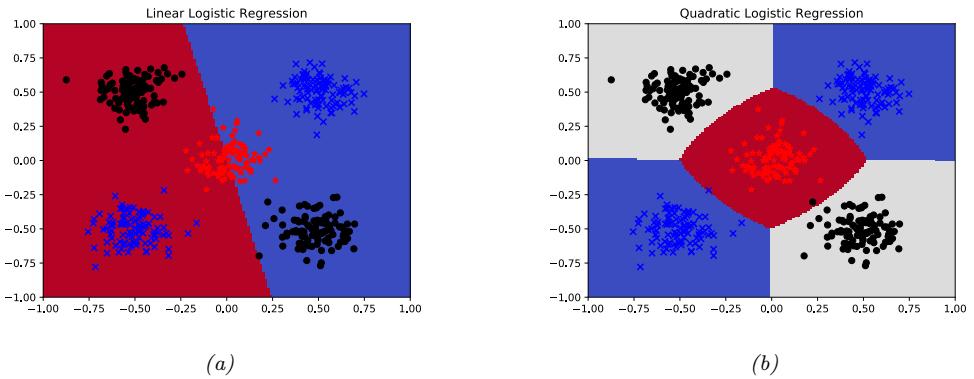
Figure 10.7: Example of 3-class logistic regression with 2d inputs. (a) Original features. (b) Quadratic features. Generated by logreg\_multiclass\_demo.ipynb.

binary logistic regression with multiple outputs:

\[p(y|x,\theta) = \prod\_{c=1}^{C} \text{Ber}(y\_c|\sigma(w\_c^\mathsf{T}x)) \tag{10.56}\]

10.3.1 Linear and nonlinear classifiers

Logistic regression computes linear decision boundaries in the input space, as shown in Figure 10.7(a) for the case where ^{x → R2} and we have ^C = 3 classes. However, we can always transform the inputs in some way to create nonlinear boundaries. For example, suppose we replace x = (x1, x2) by

\[\phi(\mathbf{x}) = [1, x\_1, x\_2, x\_1^2, x\_2^2, x\_1 x\_2] \tag{10.57}\]

This lets us create quadratic decision boundaries, as illustrated in Figure 10.7(b).

10.3.2 Maximum likelihood estimation

In this section, we discuss how to compute the maximum likelihood estimate (MLE) by minimizing the negative log likelihood (NLL).

10.3.2.1 Objective

The NLL is given by

\[\text{NLL}(\boldsymbol{\theta}) = -\frac{1}{N} \log \prod\_{n=1}^{N} \prod\_{c=1}^{C} \mu\_{nc}^{y\_{nc}} = -\frac{1}{N} \sum\_{n=1}^{N} \sum\_{c=1}^{C} y\_{nc} \log \mu\_{nc} = \frac{1}{N} \sum\_{n=1}^{N} \mathbb{H}\_{ce}(y\_n, \mu\_n) \tag{10.58}\]

where µnc = p(ync = 1|xn, ω) = softmax(f(xn, ω))c, yⁿ is the one-hot encoding of the label (so ync = I(yⁿ = c)), and Hce(yn, µn) is the cross-entropy:

\[\mathbb{H}\_{ce}(\mathbf{p}, \mathbf{q}) = -\sum\_{c=1}^{C} p\_c \log q\_c \tag{10.59}\]

10.3.2.2 Optimizing the objective

To find the optimum, we need to solve ̸wNLL(w) = 0, where w is a vectorized version of the weight matrix W, and where we are ignoring the bias term for notational simplicity. We can find such a stationary point using any gradient-based optimizer; we give some examples below. But first we derive the gradient and Hessian, and then prove that the objective is convex.

10.3.2.3 Deriving the gradient

To derive the gradient of the NLL, we need to use the Jacobian of the softmax function, which is as follows (see Exercise 10.1 for the proof):

\[\frac{\partial \mu\_c}{\partial a\_j} = \mu\_c(\delta\_{cj} - \mu\_j) \tag{10.60}\]

where ↽cj = I(c = j). For example, if we have 3 classes, the Jacobian matrix is given by

\[ \begin{bmatrix} \frac{\partial \mu\_c}{\partial a\_j} \end{bmatrix}\_{cj} = \begin{pmatrix} \mu\_1 (1 - \mu\_1) & -\mu\_1 \mu\_2 & -\mu\_1 \mu\_3 \\ -\mu\_2 \mu\_1 & \mu\_2 (1 - \mu\_2) & -\mu\_2 \mu\_3 \\ -\mu\_3 \mu\_1 & -\mu\_3 \mu\_2 & \mu\_3 (1 - \mu\_3) \end{pmatrix} \tag{10.61} \]

In matrix form, this can be written as

\[\frac{\partial \mu}{\partial \mathbf{a}} = (\mu \mathbf{1}^{\mathsf{T}}) \odot (\mathbf{I} - \mathbf{1} \boldsymbol{\mu}^{\mathsf{T}}) \tag{10.62}\]

where ^B is elementwise product, ^µ1^T copies ^µ across each column, and ¹µ^T copies ^µ across each row.

We now derive the gradient of the NLL for a single example, indexed by n. To do this, we flatten the D ↓ C weight matrix into a vector w of size CD (or (C ↑ 1)D if we freeze one of the classes to have zero weight) by concatenating the rows, and then transposing into a column vector. We use w^j to denote the vector of weights associated with class j. The gradient wrt this vector is giving by the

following (where we use the Kronecker delta notation, ↽jc, which equals 1 if j = c and 0 otherwise):

\[\nabla\_{\mathbf{w}\_j} \text{NLL}\_n = \sum\_c \frac{\partial \text{NLL}\_n}{\partial \mu\_{nc}} \frac{\partial \mu\_{nc}}{\partial a\_{nj}} \frac{\partial a\_{nj}}{\partial w\_j} \tag{10.63}\]

\[\dot{\delta} = -\sum\_{c} \frac{y\_{nc}}{\mu\_{nc}} \mu\_{nc} (\delta\_{jc} - \mu\_{nj}) x\_n \tag{10.64}\]

\[\mathbf{x} = \sum\_{c} y\_{nc} (\mu\_{nj} - \delta\_{jc}) \mathbf{x}\_n \tag{10.65}\]

\[=(\sum\_{c} y\_{nc})\mu\_{nj}\mathbf{x}\_{n} - \sum\_{c} \delta\_{jc} y\_{nj}\mathbf{x}\_{n} \tag{10.66}\]

\[=(\mu\_{nj} - y\_{nj})\mathbf{x}\_n\tag{10.67}\]

We can repeat this computation for each class, to get the full gradient vector. The gradient of the overall NLL is obtained by summing over examples, to give the D ↓ C matrix

\[\mathbf{g}(\boldsymbol{w}) = \frac{1}{N} \sum\_{n=1}^{N} \mathbf{x}\_n (\boldsymbol{\mu}\_n - \mathbf{y}\_n)^\top \tag{10.68}\]

This has the same form as in the binary logistic regression case, namely an error term times the input.

10.3.2.4 Deriving the Hessian

Exercise 10.1 asks you to show that the Hessian of the NLL for multinomial logistic regression is given by

\[\mathbf{H}(\boldsymbol{w}) = \frac{1}{N} \sum\_{n=1}^{N} (\text{diag}(\boldsymbol{\mu}\_n) - \boldsymbol{\mu}\_n \boldsymbol{\mu}\_n^\mathsf{T}) \otimes (\boldsymbol{x}\_n \boldsymbol{x}\_n^\mathsf{T}) \tag{10.69}\]

where A △ B is the Kronecker product (Section 7.2.5). In other words, the block c, c↗ submatrix is given by

\[\mathbf{H}\_{c,c'}(\mathbf{w}) = \frac{1}{N} \sum\_{n} \mu\_{nc} (\delta\_{c,c'} - \mu\_{n,c'}) x\_n \mathbf{z}\_n^{\mathsf{T}} \tag{10.70}\]

For example, if we have 3 features and 2 classes, this becomes

\[\mathbf{H}(\boldsymbol{w}) = \frac{1}{N} \sum\_{n} \begin{pmatrix} \mu\_{n1} - \mu\_{n1}^2 & -\mu\_{n1}\mu\_{n2} \\ -\mu\_{n1}\mu\_{n2} & \mu\_{n2} - \mu\_{n2}^2 \end{pmatrix} \otimes \begin{pmatrix} x\_{n1}x\_{n1} & x\_{n1}x\_{n2} & x\_{n1}x\_{n3} \\ x\_{n2}x\_{n1} & x\_{n2}x\_{n2} & x\_{n2}x\_{n3} \\ x\_{n3}x\_{n1} & x\_{n3}x\_{n2} & x\_{n3}x\_{n3} \end{pmatrix} \tag{10.71}\]

\[\mathbf{x} = \frac{1}{N} \sum\_{n} \begin{pmatrix} (\mu\_{n1} - \mu\_{n1}^2) \mathbf{X}\_n & -\mu\_{n1} \mu\_{n2} \mathbf{X}\_n \\ -\mu\_{n1} \mu\_{n2} \mathbf{X}\_n & (\mu\_{n2} - \mu\_{n2}^2) \mathbf{X}\_n \end{pmatrix} \tag{10.72}\]

where Xⁿ = xnx^{T n}. Exercise 10.1 also asks you to show that this is a positive definite matrix, so the objective is convex.

10.3.3 Gradient-based optimization

It is straightforward to use the gradient in Section 10.3.2.3 to derive the SGD algorithm. Similarly, we can use the Hessian in Section 10.3.2.4 to derive a second-order optimization method. However, computing the Hessian can be expensive, so it is common to approximate it using quasi-Newton methods, such as limited memory BFGS. (BFGS stands for Broyden, Fletcher, Goldfarb and Shanno.) See Section 8.3.2 for details. Another approach, which is similar to IRLS, is described in Section 10.3.4.

All of these methods rely on computing the gradient of the log-likelihood, which in turn requires computing normalized probabilities, which can be computed from the logits vector a = Wx using

\[p(y=c|\mathbf{z}) = \exp(a\_c - \text{lse}(\mathbf{a})) \tag{10.73}\]

where lse is the log-sum-exp function defined in Section 2.5.4. For this reason, many software libraries define a version of the cross-entropy loss that takes unnormalized logits as input.

10.3.4 Bound optimization

In this section, we consider an approach for fitting logistic regression using a class of algorithms known as bound optimization, which we describe in Section 8.7. The basic idea is to iteratively construct a lower bound on the function you want to maximize, and then to update the bound, so it “pushes up” on the true function. Optimizing the bound is often easier than updating the function directly.

If ω(ω) is a concave function we want to maximize, then one way to obtain a valid lower bound is to use a bound on its Hessian, i.e., to find a negative definite matrix B such that H(ω) ∃ B. In this case, one can show that

\[\ell(\boldsymbol{\theta}) \ge \ell(\boldsymbol{\theta}^t) + (\boldsymbol{\theta} - \boldsymbol{\theta}^t)^\mathsf{T} \boldsymbol{g}(\boldsymbol{\theta}^t) + \frac{1}{2} (\boldsymbol{\theta} - \boldsymbol{\theta}^t)^\mathsf{T} \mathbf{B} (\boldsymbol{\theta} - \boldsymbol{\theta}^t) \tag{10.74}\]

where g(ω^t ) = ̸ω(ω^t ). Defining Q(ω, ω^t ) as the right-hand-side of Equation (10.74), the update becomes

\[\boldsymbol{\theta}^{t+1} = \boldsymbol{\theta}^{t} - \mathbf{B}^{-1} \boldsymbol{g}(\boldsymbol{\theta}^{t}) \tag{10.75}\]

This is similar to a Newton update, except we use B, which is a fixed matrix, rather than H(ω^t ), which changes at each iteration. This can give us some of the advantages of second order methods at lower computational cost.

Let us now apply this to logistic regression, following [Kri+05], Let µn(w)=[p(yⁿ = 1|xn, w),…,p(yⁿ = C|xn, w)] and yⁿ = [I(yⁿ = 1),…,I(yⁿ = C)]. We want to maximize the log-likelihood, which is as follows:

\[\ell(w) = \sum\_{n=1}^{N} \left[ \sum\_{c=1}^{C} y\_{nc} w\_c^\top x\_n - \log \sum\_{c=1}^{C} \exp(w\_c^\top x\_n) \right] \tag{10.76}\]

The gradient is given by the following (see Section 10.3.2.3 for details of the derivation):

\[\mathbf{g}(\boldsymbol{w}) = \sum\_{n=1}^{N} (y\_n - \mu\_n(\boldsymbol{w})) \otimes \mathbf{z}\_n \tag{10.77}\]

where △ denotes Kronecker product (which, in this case, is just outer product of the two vectors). The Hessian is given by the following (see Section 10.3.2.4 for details of the derivation):

\[\mathbf{H}(\boldsymbol{w}) = -\sum\_{n=1}^{N} (\text{diag}(\mu\_n(\boldsymbol{w})) - \mu\_n(\boldsymbol{w})\mu\_n(\boldsymbol{w})^\mathsf{T}) \otimes (\boldsymbol{x}\_n \boldsymbol{x}\_n^\mathsf{T})\tag{10.78}\]

We can construct a lower bound on the Hessian, as shown in [Boh92]:

\[\mathbf{H}(\boldsymbol{w}) \succ -\frac{1}{2} [\mathbf{I} - \mathbf{1}\mathbf{1}^{\mathsf{T}}/C] \otimes \left(\sum\_{n=1}^{N} \boldsymbol{x}\_{n} \boldsymbol{x}\_{n}^{\mathsf{T}}\right) \triangleq \mathbf{B} \tag{10.79}\]

where I is a C-dimensional identity matrix, and 1 is a C-dimensional vector of all 1s.1 In the binary case, this becomes

\[\mathbf{H}(\mathbf{w}) \succ -\frac{1}{2}\left(1 - \frac{1}{2}\right)\left(\sum\_{n=1}^{N} \mathbf{x}\_n \mathbf{z}\_n^\top\right) = -\frac{1}{4}\mathbf{X}^\top \mathbf{X} \tag{10.80}\]

This follows since ^µn ↘ ⁰.⁵ so ^↑(µ^{n ↑ µ2 n}) ∋ ↑0.25.

We can use this lower bound to construct an MM algorithm to find the MLE. The update becomes

\[w^{t+1} = w^t - \mathbf{B}^{-1} g(w^t) \tag{10.81}\]

This iteration can be faster than IRLS (Section 10.2.6) since we can precompute B→¹ in time independent of N, rather than having to invert the Hessian at each iteration. For example, let us consider the binary case, so ^{gt =} ̸ω(w^t ) = ^XT(^{y ↑ µt} ), where µ^t = [pn(w^t ),(1 ^{↑ p}n(w^t ))]^{N n}=1. The update becomes

\[w^{t+1} = w^t - 4(\mathbf{X}^\mathsf{T}\mathbf{X})^{-1}g^t\tag{10.82}\]

Compare this to Equation (10.37), which has the following form:

\[\boldsymbol{w}^{t+1} = \boldsymbol{w}^t - \mathbf{H}^{-1} \boldsymbol{g}(\boldsymbol{w}^t) = \boldsymbol{w}^t - (\mathbf{X}^\mathsf{T} \mathbf{S}^t \mathbf{X})^{-1} \boldsymbol{g}^t \tag{10.83}\]

where S^t = diag(µ^{t B}(1 ^{↑ µt} )). We see that Equation (10.82) is faster to compute, since we can precompute the constant matrix (X^TX)→¹.

10.3.5 MAP estimation

In Section 10.2.7 we discussed the benefits of ω² regularization for binary logistic regression. These benefits hold also in the multi-class case. However, there is also an additional, and surprising, benefit to do with identifiability of the parameters, as pointed out in [HTF09, Ex.18.3]. (We say that the parameters are identifiable if there is a unique value that maximizes the likelihood; equivalently, we require that the NLL be strictly convex.)

^1. If we enforce that w^C = 0, we can use C ↔︎ 1 dimensions for these vectors / matrices.

To see why identifiability is an issue, recall that multiclass logistic regression has the form

\[p(y = c | \mathbf{x}, \mathbf{W}) = \frac{\exp(\mathbf{w}\_c^T \mathbf{x})}{\sum\_{k=1}^C \exp(\mathbf{w}\_k^T \mathbf{x})} \tag{10.84}\]

where W is a C ↓ D weight matrix. We can arbitrarily define w^c = 0 for one of the classes, say ^{c = C}, since ^p(^{y = C}|x,W)=1 ^↑ $C→^{1 c}=1 p(y = c|x, w). In this case, the model has the form

\[p(y = c | \mathbf{x}, \mathbf{W}) = \frac{\exp(\mathbf{w}\_c^T \mathbf{x})}{1 + \sum\_{k=1}^{C-1} \exp(\mathbf{w}\_k^T \mathbf{x})} \tag{10.85}\]

If we don’t “clamp” one of the vectors to some constant value, the parameters will be unidentifiable.

However, suppose we don’t clamp w^c = 0, so we are using Equation 10.84, but we add ω² regularization by optimizing

\[\text{PNLL}(\mathbf{W}) = -\sum\_{n=1}^{N} \log p(y\_n | \mathbf{x}\_n, \mathbf{W}) + \lambda \sum\_{c=1}^{C} ||\mathbf{w}\_c||\_2^2 \tag{10.86}\]

where we have absorbed the 1/N term into φ. At the optimum we have $^{C c}=1 wˆcj = 0 for j =1: D, so the weights automatically satisfy a sum-to-zero constraint, thus making them uniquely identifiable.

To see why, note that at the optimum we have

\[\nabla \text{NLL}(w) + 2\lambda w = 0\tag{10.87}\]

\[\sum\_{n} (y\_n - \mu\_n) \otimes x\_n = \lambda w \tag{10.88}\]

Hence for any feature dimension j we have

\[ \lambda \sum\_{c} w\_{cj} = \sum\_{n} \sum\_{c} (y\_{nc} - \mu\_{nc}) x\_{nj} = \sum\_{n} (\sum\_{c} y\_{nc} - \sum\_{c} \mu\_{nc}) x\_{nj} = \sum\_{n} (1 - 1) x\_{nj} = 0 \tag{10.89} \]

Thus if φ > 0 we have $ ^c wˆcj = 0, so the weights will sum to zero across classes for each feature dimension.

10.3.6 Maximum entropy classifiers

Recall that the multinomial logistic regression model can be written as

\[p(y = c | \mathbf{x}, \mathbf{W}) = \frac{\exp(\mathbf{w}\_c^\mathsf{T} \mathbf{x})}{Z(\mathbf{w}, \mathbf{x})} = \frac{\exp(\mathbf{w}\_c^\mathsf{T} \mathbf{x})}{\sum\_{c'=1}^C \exp(\mathbf{w}\_{c'}^\mathsf{T} \mathbf{x})} \tag{10.90}\]

where Z(w, x) = $ ^c exp(w^{T c}x) is the partition function (normalization constant). This uses the same features, but a di!erent weight vector, for every class. There is a slight extension of this model that allows us to use features that are class-dependent. This model can be written as

\[p(y=c|x,w) = \frac{1}{Z(w,x)} \exp(w^\top \phi(x,c))\tag{10.91}\]

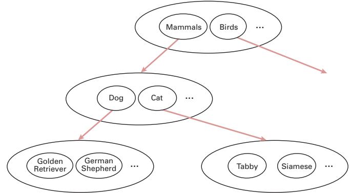
Figure 10.8: A simple example of a label hierarchy. Nodes within the same ellipse have a mutual exclusion relationship between them.

where ϑ(x, c) is the feature vector for class c. This is called a maximum entropy classifer, or maxent classifier for short. (The origin of this term is explained in Section 3.4.4.)

Maxent classifiers include multinomial logistic regression as a special case. To see this let w = [w1,…, w^C ], and define the feature vector as follows:

\[\phi(x,c) = [\mathbf{0}, \dots, x, \dots, \mathbf{0}] \tag{10.92}\]

where x is embedded in the c’th block, and the remaining blocks are zero. In this case, w^Tϑ(x, c) = w^{T c}x, so we recover multinomial logistic regression.

Maxent classifiers are very widely used in the field of natural language processing. For example, consider the problem of semantic role labeling, where we classify a word x into a semantic role y, such as person, place or thing. We might define (binary) features such as the following:

\[\phi\_1(\mathbf{z}, y) = \mathbb{I}\left(y = \text{person} \land \mathbf{z} \text{ occurs after "Mr" or "Mr"}\right) \tag{10.93}\]

\[\phi\_2(\mathbf{z}, y) = \mathbb{I}\left(y = \text{person} \land \mathbf{z} \text{ is in whitelist of common names}\right) \tag{10.94}\]

\[\phi\_3(\mathbf{z}, y) = \mathbb{I}\left(y = \text{place} \land \mathbf{z} \text{ is in Google maps}\right) \tag{10.95}\]

We see that the features we use depend on the label.

There are two main ways of creating these features. The first is to manually specify many possibly useful features using various templates, and then use a feature selection algorithm, such as the group lasso method of Section 11.4.7. The second is to incrementally add features to the model, using a heuristic feature generation method.

10.3.7 Hierarchical classification

. . .

Sometimes the set of possible labels can be structured into a hierarchy or taxonomy. For example, we might want to predict what kind of an animal is in an image: it could be a dog or a cat; if it is a

dog, it could be a golden retriever or a German shepherd, etc. Intuitively, it makes sense to try to predict the most precise label for which we are confident [Den+12], that is, the system should “hedge its bets”.

One simple way to achieve this, proposed in [RF17], is as follows. First, create a model with a binary output label for every possible node in the tree. Before training the model, we will use label smearing, so that a label is propagated to all of its parents (hypernyms). For example, if an image is labeled “golden retriever”, we will also label it “dog”. If we train a multi-label classifier (which produces a vector p(y|x) of binary labels) on such smeared data, it will perform hierarchical classification, predicting a set of labels at di!erent levels of abstraction.

However, this method could predict “golden retriever”, “cat” and “bird” all with probability 1.0, since the model does not capture the fact that some labels are mutually exclusive. To prevent this, we can add a mutual exclusion constraint between all label nodes which are siblings, as shown in Figure 10.8. For example, this model enforces that p(mammal|x) + p(bird|x)=1, since these two labels are children of the root node. We can further partition the mammal probability into dogs and cats, so we have p(dog|x) + p(cat|x) = p(mammal|x).

[Den+14; Din+15] generalize the above method by using a conditional graphical model where the graph structure can be more complex than a tree. In addition, they allow for soft constraints between labels, in addition to hard constraints.

10.3.8 Handling large numbers of classes

In this section, we discuss some issues that arise when there are a large number of potential labels, e.g., if the labels correspond to words from a language.

10.3.8.1 Hierarchical softmax

In regular softmax classifiers, computing the normalization constant, which is needed to compute the gradient of the log likelihood, takes O(C) time, which can become the bottleneck if C is large. However, if we structure the labels as a tree, we can compute the probability of any label in O(log C) time, by multiplying the probabilities of each edge on the path from the root to the leaf. For example, consider the tree in Figure 10.9. We have

\[p(y = \text{I'm}|C) = 0.57 \times 0.68 \times 0.72 = 0.28 \tag{10.96}\]

Thus we replace the “flat” output softmax with a tree-structured sequence of binary classifiers. This is called hierarchical softmax [Goo01; MB05].

A good way to structure such a tree is to use Hu!man encoding, where the most frequent labels are placed near the top of the tree, as suggested in [Mik+13a]. (For a di!erent appproach, based on clustering the most common labels together, see [Gra+17]. And for yet another approach, based on sampling labels, see [Tit16].)

10.3.8.2 Class imbalance and the long tail

Another issue that often arises when there are a large number of classes is that for most classes, we may have very few examples. More precisely, if N^c is the number of examples of class c, then the empirical distribution p(N1,…,N^C ) may have a long tail. The result is an extreme form of class

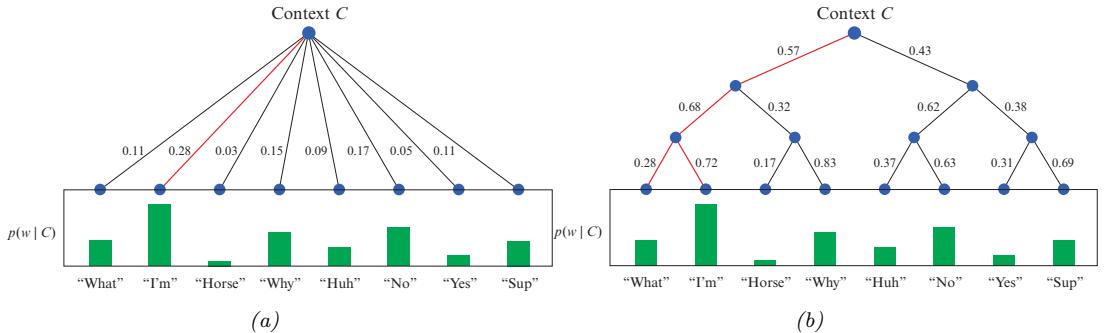
Figure 10.9: A flat and hierarchical softmax model p(w|C), where C are the input features (context) and w is the output label (word). Adapted from https: // www. quora. com/ What-is-hierarchical-softmax .

imbalance (see e.g., [ASR15]). Since the rare classes will have a smaller e!ect on the overall loss than the common classes, the model may “focus its attention” on the common classes.

One method that can help is to set the bias terms b such that softmax(b)^c = Nc/N; such a model will match the empirical label prior even when using weights of w = 0. We can then “subtract o!” the prior term by using logit adjustment [Men+21], which ensures good performance across all groups.

Another common approach is to resample the data to make it more balanced, before (or during) training. In particular, suppose we sample a datapoint from class c with probability

\[p\_c = \frac{N\_c^q}{\sum\_{i}^{C} N\_i^q} \tag{10.97}\]

If we set q = 1, we recover standard instance-balanced sampling, where p^c ∞ Nc; the common classes will be sampled more than rare classes. If we set q = 0, we recover class-balanced sampling, where p^c = 1/C; this can be thought of as first sampling a class uniformly at random, and then sampling an instance of this class. Finally, we can consider other options, such as q = 0.5, which is known as square-root sampling [Mah+18].

Yet another method that is simple and can easily handle the long tail is to use the nearest class mean classifier. This has the form

\[f(\mathbf{x}) = \operatorname\*{argmin}\_{\mathbf{c}} ||\mathbf{x} - \boldsymbol{\mu}\_{\mathbf{c}}||\_2^2 \tag{10.98}\]

where µ^c = ¹ N^c $ ⁿ:yn=^c xⁿ is the mean of the features belonging to class c. This induces a softmax posterior, as we discussed in Section 9.2.5. We can get much better results if we first use a neural network (see Part III) to learn good features, by training a DNN classifier with cross-entropy loss on the original unbalanced data. We then replace x with ϑ(x) in Equation (10.98). This simple approach can give very good performance on long-tailed distributions [Kan+20].

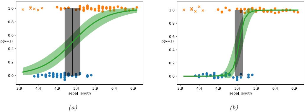
Figure 10.10: (a) Logistic regression on some data with outliers (denoted by x). Training points have been (vertically) jittered to avoid overlapping too much. Vertical line is the decision boundary, and its posterior credible interval. (b) Same as (a) but using robust model, with a mixture likelihood. Adapted from Figure 4.13 of [Mar18]. Generated by logreg\_iris\_bayes\_robust\_1d\_pymc3.ipynb.

10.4 Robust logistic regression *

Sometimes we have outliers in our data, which are often due to labeling errors, also called label noise. To prevent the model from being adversely a!ected by such contamination, we will use robust logistic regression. In this section, we discuss some approaches to this problem. (Note that the methods can also be applied to DNNs. For a more thorough survey of label noise, and how it impacts deep learning, see [Han+20].)

10.4.1 Mixture model for the likelihood

One of the simplest ways to define a robust logistic regression model is to modify the likelihood so that it predicts that each output label y is generated uniformly at random with probability ϑ, and otherwise is generated using the usual conditional model. In the binary case, this becomes

\[p(y|\mathbf{z}) = \pi \text{Ber}(y|0.5) + (1 - \pi) \text{Ber}(y|\sigma(\mathbf{w}^\top \mathbf{z})) \tag{10.99}\]

This approach, of using a mixture model for the observation model to make it robust, can be applied to many di!erent models (e.g., DNNs).

We can fit this model using standard methods, such as SGD or Bayesian inference methods such as MCMC. For example, let us create a “contaminated” version of the 1d, two-class Iris dataset that we discussed in Section 4.6.7.2. We will add 6 examples of class 1 (Versicolor) with abnormally low sepal length. In Figure 10.10a, we show the results of fitting a standard (Bayesian) logistic regression model to this dataset. In Figure 10.10b, we show the results of fitting the above robust model. In the latter case, we see that the decision boundary is similar to the one we inferred from non-contaminated data, as shown in Figure 4.20b. We also see that the posterior uncertainty about the decision boundary’s location is smaller than when using a non-robust model.

10.4.2 Bi-tempered loss

In this section, we present an approach to robust logistic regression proposed in [Ami+19].

The first observation is that examples that are far from the decision boundary, but mislabeled, will have undue adverse a!ect on the model if the loss function is convex [LS10]. This can be overcome by replacing the usual cross entropy loss with a “tempered” version, that uses a temperature parameter 0 ↘ t¹ < 1 to ensure the loss from outliers is bounded. In particular, consider the standard relative entropy loss function:

\[\mathcal{L}(\boldsymbol{y}, \hat{\boldsymbol{y}}) = \mathbb{H}\_{ce}(\boldsymbol{y}, \hat{\boldsymbol{y}}) = \sum\_{c} y\_{c} \log \hat{y}\_{c} \tag{10.100}\]

where y is the true label distribution (often one-hot) and yˆ is the predicted distribution. We define the tempered cross entropy loss as follows:

\[\mathcal{L}(\mathbf{y}, \hat{\mathbf{y}}) = \sum\_{c} \left[ y\_c (\log\_{t\_1} y\_c - \log\_{t\_1} \hat{y}\_c) - \frac{1}{2 - t\_1} (y\_c^{2 - t\_1} - \hat{y}\_c^{2 - t\_1}) \right] \tag{10.101}\]

which simplifes to the following when the true distribution y is one-hot, with all its mass on class c:

\[\mathcal{L}(c, \hat{\mathbf{y}}) = -\log\_{t\_1} \hat{y}\_c - \frac{1}{2 - t\_1} \left( 1 - \sum\_{c'=1}^C \hat{y}\_{c'}^{2 - t\_1} \right) \tag{10.102}\]

Here log^t is tempered version of the log function:

\[\log\_t(x) \stackrel{\Delta}{=} \frac{1}{1-t}(x^{1-t}-1) \tag{10.103}\]

This is mononotically increasing and concave, and reduces to the standard (natural) logarithm when t = 1. (Similarly, tempered cross entropy reduces to standard cross entropy when t = 1.) However, the tempered log function is bounded from below by ↑1/(1 ↑ t) for 0 ↘ t < 1, and hence the cross entropy loss is bounded from above (see Figure 10.11).

The second observation is that examples that are near the decision boundary, but mislabeled, need to use a transfer function (that maps from activations R^C to probabilities [0, 1]^C ) that has heavier tails than the softmax, which is based on the exponential, so it can “look past” the neighborhood of the immediate examples. In particular, the standard softmax is defined by

\[\hat{y}\_c = \frac{a\_c}{\sum\_{c'=1}^C \exp(a\_{c'})} = \exp\left[a\_c - \log \sum\_{c'=1}^C \exp(a\_{c'})\right] \tag{10.104}\]

where a is the logits vector. We can make a heavy tailed version by using the tempered softmax, which uses a temperature parameter t² > 1 > t¹ as follows:

\[ \hat{y}\_c = \exp\_{t\_2}(a\_c - \lambda\_{t\_2}(\mathbf{a})) \tag{10.105} \]

where

\[\exp\_t(x) \triangleq \left[1 + (1 - t)x\right]\_+^{1/(1-t)}\tag{10.106}\]

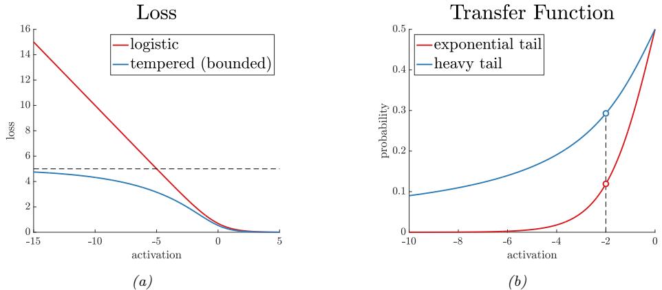
Figure 10.11: (a) Illustration of logistic and tempered logistic loss with t¹ = 0.8. (b) Illustration of sigmoid and tempered sigmoid transfer function with t² = 2.0. From https: // ai. googleblog. com/ 2019/ 08/ bi-tempered-logistic-loss-for-training. html . Used with kind permission of Ehsan Amid.

is a tempered version of the exponential function. (This reduces to the standard exponental function as t ↔︎ 1.) In Figure 10.11(right), we show that the tempered softmax (in the two-class case) has heavier tails, as desired.

All that remains is a way to compute φ^t2 (a). This must satisfy the following fixed point equation:

\[\sum\_{c=1}^{C} \exp\_{t\_2}(a\_c - \lambda(\mathbf{a})) = 1\tag{10.107}\]

We can solve for φ using binary search, or by using the iterative procedure in Algorithm 10.2.

Algorithm 10.2: Iterative algorithm for computing φ(a) in Equation (10.107). From [AWS19].

Input: logits a, temperature t > 1 µ := max(a) a := a ↑ µ while a not converged do Z(a) := $^{C c}=1 expt(ac) a := Z(a)¹→^t (a ↑ µ1) Return ^↑ log^{t 1 Z}(a) + µ

Combining the tempered softmax with the tempered cross entropy results in a method called bi-tempered logistic regression. In Figure 10.12, we show an example of this in 2d. The top row is standard logistic regression, the bottom row is bi-tempered. The first column is clean data. The second column has label noise near the boundary. The robust version uses t¹ = 1 (standard cross entropy) but t² = 4 (tempered softmax with heavy tails). The third column has label noise far

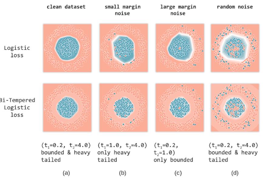
Figure 10.12: Illustration of standard and bi-tempered logistic regression on data with label noise. From https: // ai. googleblog. com/ 2019/ 08/ bi-tempered-logistic-loss-for-training. html . Used with kind permission of Ehsan Amid.

from the boundary. The robust version uses t¹ = 0.2 (tempered cross entropy with bounded loss) but t² = 1 (standard softmax). The fourth column has both kinds of noise; in this case, the robust version uses t¹ = 0.2 and t² = 4.

10.5 Bayesian logistic regression *

So far we have focused on point estimates of the parameters, either the MLE or the MAP estimate. However, in some cases we want to compute the posterior, p(w|D), in order to capture our uncertainty. This can be particularly useful in settings where we have little data, and where choosing the wrong decision may be costly.

Unlike with linear regression, it is not possible to compute the posterior exactly for a logistic regression model. A wide range of approximate algorithms can be used,. In this section, we use one of the simplest, known as the Laplace approximation (Section 4.6.8.2). See the sequel to this book, [Mur23] for more advanced approximations.

10.5.1 Laplace approximation

As we discuss in Section 4.6.8.2, the Laplace approximation approximates the posterior using a Gaussian. The mean of the Gaussian is equal to the MAP estimate wˆ , and the covariance is equal to the inverse Hessian H computed at the MAP estimate, i.e., ^p(w|D) ↖ ^N (w|w^ˆ , H→¹), We can find the mode using a standard optimization method (see Section 10.2.7), and then we can use the results

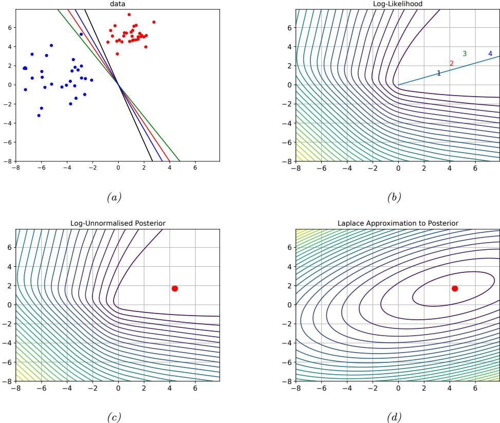
Figure 10.13: (a) Illustration of the data. (b) Log-likelihood for a logistic regression model. The line is drawn from the origin in the direction of the MLE (which is at infinity). The numbers correspond to 4 points in parameter space, corresponding to the lines in (a). (c) Unnormalized log posterior (assuming vague spherical prior). (d) Laplace approximation to posterior. Adapted from a figure by Mark Girolami. Generated by logreg\_laplace\_demo.ipynb.

from Section 10.2.3.4 to compute the Hessian at the mode.

As an example, consider the data illustrated in Figure 10.13(a). There are many parameter settings that correspond to lines that perfectly separate the training data; we show 4 example lines. The likelihood surface is shown in Figure 10.13(b). The diagonal line connects the origin to the point in the grid with maximum likelihood, wˆ mle = (8.0, 3.4). (The unconstrained MLE has ||w|| = ∈, as we discussed in Section 10.2.7; this point can be obtained by following the diagonal line infinitely far to the right.)

For each decision boundary in Figure 10.13(a), we plot the corresponding parameter vector in Figure 10.13(b). These parameters values are w¹ = (3, 1), w² = (4, 2), w³ = (5, 3), and w⁴ = (7, 3). These points all approximately satisfy wi(1)/wi(2) ↖ wˆ mle(1)/wˆ mle(2), and hence are close to the

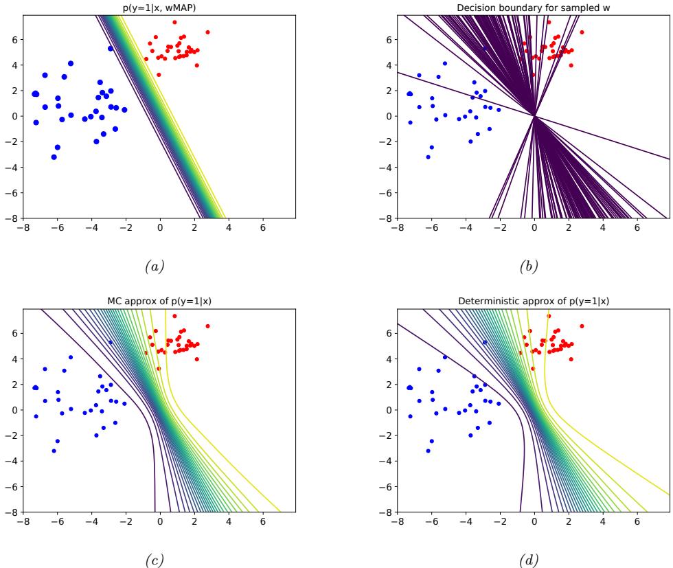
Figure 10.14: Posterior predictive distribution for a logistic regression model in 2d. (a): contours of p(y = 1|x, wˆ map). (b): samples from the posterior predictive distribution. (c): Averaging over these samples. (d): moderated output (probit approximation). Adapted from a figure by Mark Girolami. Generated by logreg\_laplace\_demo.ipynb.

orientation of the maximum likelihood decision boundary. The points are ordered by increasing weight norm (3.16, 4.47, 5.83, and 7.62).

To ensure a unique solution, we use a (spherical) Gaussian prior centered at the origin, ^N (w|0, ^ε2I). The value of ε² controls the strength of the prior. If we set ε² = 0, we force the MAP estimate to be w = 0; this will result in maximally uncertain predictions, since all points x will produce a predictive distribution of the form ^p(^y = 1|x)=0.5. If we set ^ε2 = ^∈, the prior becomes uninformative, and MAP estimate becomes the MLE, resulting in minimally uncertain predictions. (In particular, all positively labeled points will have p(y = 1|x)=1.0, and all negatively labeled points will have p(y = 1|x)=0.0, since the data is separable.) As a compromise (to make a nice illustration), we pick the value ε² = 100.

Multiplying this prior by the likelihood results in the unnormalized posterior shown in Fig-

ure 10.13(c). The MAP estimate is shown by the red dot. The Laplace approximation to this posterior is shown in Figure 10.13(d). We see that it gets the mode correct (by construction), but the shape of the posterior is somewhat distorted. (The southwest-northeast orientation captures uncertainty about the magnitude of w, and the southeast-northwest orientation captures uncertainty about the orientation of the decision boundary.)

In Figure 10.14, we show contours of the posterior predictive distribution. Figure 10.14(a) shows the plugin approximation using the MAP estimate. We see that there is no uncertainty about the decision boundary, even though we are generating probabilistic predictions over the labels. Figure 10.14(b) shows what happens when we plug in samples from the Gaussian posterior. Now we see that there is considerable uncertainty about the orientation of the “best” decision boundary. Figure 10.14(c) shows the average of these samples. By averaging over multiple predictions, we see that the uncertainty in the decision boundary “splays out” as we move further from the training data. Figure 10.14(d) shows that the probit approximation gives very similar results to the Monte Carlo approximation.

10.5.2 Approximating the posterior predictive

The posterior p(w|D) tells us everything we know about the parameters of the model given the data. However, in machine learning applications, the main task of interest is usually to predict an output y given an input x, rather than to try to understand the parameters of our model. Thus we need to compute the posterior predictive distribution

\[p(y|\mathbf{z}, \mathcal{D}) = \int p(y|\mathbf{z}, \mathbf{w}) p(\mathbf{w}|\mathcal{D}) d\mathbf{w} \tag{10.108}\]

As we discussed in Section 4.6.7.1, a simple approach to this is to first compute a point estimate wˆ of the parameters, such as the MLE or MAP estimate, and then to ignore all posterior uncertainty, by assuming p(w|D) = ↽(w ↑ wˆ ). In this case, the above integral reduces to the following plugin approximation:

\[p(y|x,\mathcal{D}) \approx \int p(y|x,w)\delta(w-\hat{w})dw = p(y|x,\hat{w})\tag{10.109}\]

However, if we want to compute uncertainty in our predictions, we should use a non-degenerate posterior. It is common to use a Gaussian posterior, as we will see. But we still need to approximate the integral in Equation (10.108). We discuss some approaches to this below.

10.5.2.1 Monte Carlo approximation

The simplest approach is to use a Monte Carlo approximation to the integral. This means we draw S samples from the posterior, w^s ⇒ p(w|D). and then compute

\[p(y=1|\mathbf{x}, \mathcal{D}) \approx \frac{1}{S} \sum\_{s=1}^{S} \sigma(w\_s^{\mathsf{T}} \mathbf{x}) \tag{10.110}\]

10.5.2.2 Probit approximation

Although the Monte Carlo approximation is simple, it can be slow, since we need to draw S samples at test time for each input x. Fortunately, if p(w|D) = N (w|µ, !), there is a simple yet accurate

deterministic approximation, first suggested in [SL90]. To explain this approximation, we follow the presentation of [Bis06, p219]. The key observation is that the sigmoid function ε(a) is similar in shape to the Gaussian cdf (see Section 2.6.1) !(a). In particular we have ε(a) ↖ !(φa), where φ² = ϑ/8 ensures the two functions have the same slope at the origin. This is useful since we can integrate a Gaussian cdf wrt a Gaussian pdf exactly:

\[\int \Phi(\lambda a) N(a|m,v) da = \Phi\left(\frac{m}{(\lambda^{-2} + v)^{\frac{1}{2}}}\right) = \Phi\left(\frac{\lambda m}{(1 + \lambda^2 v)^{\frac{1}{2}}}\right) \approx \sigma(\kappa(v)m) \tag{10.111}\]

where we have defined

\[\kappa(v) \stackrel{\Delta}{=} (1 + \pi v/8)^{-\frac{1}{2}} \tag{10.112}\]

Thus if we define a = x^Tw, we have

\[p(y=1|\mathcal{D}, \mathcal{D}) \approx \sigma(\kappa(v)m) \tag{10.113}\]

\[m = \mathbb{E}\left[a\right] = \mathbf{x}^{\mathsf{T}}\boldsymbol{\mu}\tag{10.114}\]

\[v = \mathbb{V}\left[a\right] = \mathbb{V}\left[\boldsymbol{x}^{\mathsf{T}}\boldsymbol{w}\right] = \boldsymbol{x}^{\mathsf{T}}\boldsymbol{\Sigma}\boldsymbol{x} \tag{10.115}\]

where we used Equation (2.165) in the last line. Since ! is the inverse of the probit function, we will call this the probit approximation.

Using Equation (10.113) results in predictions that are less extreme (in terms of their confidence) than the plug-in estimate. To see this, note that 0 < 2(v) < 1 and hence 2(v)m<m, so ε(2(v)m) is closer to 0.5 than ε(m) is. However, the decision boundary itself will not be a!ected. To see this, note that the decision boundary is the set of points x for which p(y = 1|x, D)=0.5. This implies 2(v)m = 0, which implies m = w^Tx = 0; but this is the same as the decision boundary from the plugin estimate. Thus “being Bayesian” doesn’t change the misclassification rate (in this case), but it does change the confidence estimates of the model, which can be important, as we illustrate in Section 10.5.1.

In the multiclass case we can use the generalized probit approximation [Gib97]:

\[p(y = c | \mathbf{z}, \mathcal{D}) \approx \frac{\exp(\kappa \langle v\_c \rangle m\_c)}{\sum\_{c'} \exp(\kappa \langle v\_{c'} \rangle m\_{c'})} \tag{10.116}\]

\[m\_c = \overline{m}\_c^\dagger \underline{x} \tag{10.117}\]

\[v\_c = x^\top \mathbf{V}\_{c,c} x \tag{10.118}\]

where 2 is defined in Equation (10.112). Unlike the binary case, taking into account posterior covariance gives di!erent predictions than the plug-in approach (see Exercise 3.10.3 of [RW06]).

For further approximations of Gaussian integrals combined with sigmoid and softmax functions, see [Dau17].

10.6 Exercises

Exercise 10.1 [Gradient and Hessian of log-likelihood for multinomial logistic regression] a. Let µik = softmax(ϖi)k, where ϖⁱ = w^T xi. Show that the Jacobian of the softmax is

\[\frac{\partial \mu\_{ik}}{\partial \eta\_{lj}} = \mu\_{ik}(\delta\_{kj} - \mu\_{ij}) \tag{10.119}\]

where ◁kj = I(k = j).

2. Hence show that the gradient of the NLL is given by

\[\nabla\_{\mathbf{w}\_{c}}\ell = \sum\_{i} (y\_{ic} - \mu\_{ic})\mathbf{z}\_{i} \tag{10.120}\]

Hint: use the chain rule and the fact that ! ^c yic = 1.

3. Show that the block submatrix of the Hessian for classes c and c^↓ is given by

\[\mathbf{H}\_{c,c'} = -\sum\_{i} \mu\_{ic} (\delta\_{c,c'} - \mu\_{i,c'}) \mathbf{x}\_i \mathbf{x}\_i^T \tag{10.121}\]

Hence show that the Hessian of the NLL is positive definite.

Exercise 10.2 [Regularizing separate terms in 2d logistic regression † ] (Source: Jaakkola.)

• 1. Consider the data in Figure 10.15a, where we fit the model p(y = 1|x, w) = ϑ(w⁰ +w1x¹ +w2x2). Suppose we fit the model by maximum likelihood, i.e., we minimize

\[J(w) = -\ell(w, \mathcal{D}\_{\text{train}}) \tag{10.122}\]

where ,(w, Dtrain) is the log likelihood on the training set. Sketch a possible decision boundary corresponding to wˆ . (Copy the figure first (a rough sketch is enough), and then superimpose your answer on your copy, since you will need multiple versions of this figure). Is your answer (decision boundary) unique? How many classification errors does your method make on the training set?

2. Now suppose we regularize only the w⁰ parameter, i.e., we minimize

\[J\_0(\mathbf{w}) = -\ell(\mathbf{w}, \mathcal{D}\_{\text{train}}) + \lambda w\_0^2 \tag{10.123}\]

Suppose ↼ is a very large number, so we regularize w⁰ all the way to 0, but all other parameters are unregularized. Sketch a possible decision boundary. How many classification errors does your method make on the training set? Hint: consider the behavior of simple linear regression, w⁰ + w1x¹ + w2x² when x¹ = x² = 0.

3. Now suppose we heavily regularize only the w¹ parameter, i.e., we minimize

\[J\_1(\mathbf{w}) = -\ell(\mathbf{w}, \mathcal{D}\_{\text{train}}) + \lambda w\_1^2 \tag{10.124}\]

Sketch a possible decision boundary. How many classification errors does your method make on the training set?

4. Now suppose we heavily regularize only the w² parameter. Sketch a possible decision boundary. How many classification errors does your method make on the training set?

Exercise 10.3 [Logistic regression vs LDA/QDA † ]

(Source: Jaakkola.) Suppose we train the following binary classifiers via maximum likelihood.

• 1. GaussI: A generative classifier, where the class-conditional densities are Gaussian, with both covariance matrices set to I (identity matrix), i.e., p(x|y = c) = N (x|µc, I). We assume p(y) is uniform.
• 2. GaussX: as for GaussI, but the covariance matrices are unconstrained, i.e., p(x|y = c) = N (x|µc, !c).
• 3. LinLog: A logistic regression model with linear features.

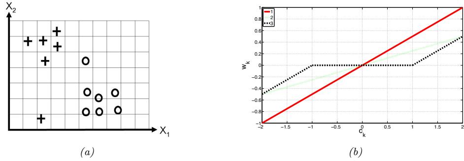
Figure 10.15: (a) Data for logistic regression question. (b) Plot of wˆ^k vs amount of correlation c^k for three di!erent estimators.

4. QuadLog: A logistic regression model, using linear and quadratic features (i.e., polynomial basis function expansion of degree 2).

After training we compute the performance of each model M on the training set as follows:

\[L(M) = \frac{1}{n} \sum\_{i=1}^{n} \log p(y\_i | \mathbf{x}\_i, \hat{\theta}, M) \tag{10.125}\]

(Note that this is the conditional log-likelihood ^p(y|x, ^ωˆ) and not the joint log-likelihood ^p(y, ^x|ωˆ).) We now want to compare the performance of each model. We will write L(M) ↗ L(M^↓ ) if model M must have lower (or equal) log likelihood (on the training set) than M^↓ , for any training set (in other words, M is worse than M^↓ , at least as far as training set logprob is concerned). For each of the following model pairs, state whether L(M) ↗ L(M^↓ ), L(M) ↖ L(M^↓ ), or whether no such statement can be made (i.e., M might sometimes be better than M^↓ and sometimes worse); also, for each question, briefly (1-2 sentences) explain why.

• 1. GaussI, LinLog.
• 2. GaussX, QuadLog.
• 3. LinLog, QuadLog.
• 4. GaussI, QuadLog.
• 5. Now suppose we measure performance in terms of the average misclassification rate on the training set:

\[R(M) = \frac{1}{n} \sum\_{i=1}^{n} I(y\_i \neq \hat{y}(\mathbf{z}\_i)) \tag{10.126}\]

Is it true in general that L(M) > L(M^↓ ) implies that R(M) < R(M^↓ )? Explain why or why not.

11 Linear Regression

11.1 Introduction

In this chapter, we discuss linear regression, which is a very widely used method for predicting a real-valued output (also called the dependent variable or target) y → R, given a vector of real-valued inputs (also called independent variables, explanatory variables, or covariates) ^{x → RD}. The key property of the model is that the expected value of the output is assumed to be a linear function of the input, ^E [y|x] ^{= wT}x, which makes the model easy to interpret, and easy to fit to data. We discuss nonlinear extensions later in this book.

11.2 Least squares linear regression

In this section, we discuss the most common form of linear regression model.

11.2.1 Terminology

The term “linear regression” usually refers to a model of the following form:

\[p(y|x,\theta) = \mathcal{N}(y|w\_0 + \mathbf{w}^\top x, \sigma^2) \tag{11.1}\]

where ω = (w0, w, ε²) are all the parameters of the model. (In statistics, the parameters w⁰ and w are usually denoted by 1⁰ and ε.)

The vector of parameters w1:^D are known as the weights or regression coe!cients. Each coe”cient w^d specifies the change in the output we expect if we change the corresponding input feature x^d by one unit. For example, suppose x¹ is the age of a person, x² is their education level (represented as a continuous number), and y is their income. Thus w¹ corresponds to the increase in income we expect as someone becomes one year older (and hence get more experience), and w² corresponds to the increase in income we expect as someone’s education level increases by one level. The term w⁰ is the o”set or bias term, and specifies the output value if all the inputs are 0. This captures the unconditional mean of the response, w⁰ = E [y], and acts as a baseline. We will usually assume that x is written as [1, x1,…,xD], so we can absorb the o!set term w⁰ into the weight vector w.

If the input is one-dimensional (so D = 1), the model has the form f(x; w) = ax + b, where b = w⁰ is the intercept, and a = w¹ is the slope. This is called simple linear regression. If the input is multi-dimensional, ^{x → RD} where D > ¹, the method is called multiple linear regression. If the

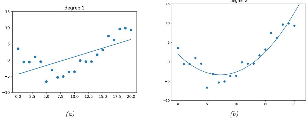
Figure 11.1: Polynomial of degrees 1 and 2 fit to 21 datapoints. Generated by linreg\_poly\_vs\_degree.ipynb.

output is also multi-dimensional, ^{y → RJ} , where J > ¹, it is called multivariate linear regression,

\[p(\mathbf{y}|\mathbf{z}, \mathbf{W}) = \prod\_{j=1}^{J} \mathcal{N}(y\_j|\mathbf{w}\_j^\mathsf{T}\mathbf{z}, \sigma\_j^2) \tag{11.2}\]

See Exercise 11.1 for a simple numerical example.

In general, a straight line will not provide a good fit to most data sets. However, we can always apply a nonlinear transformation to the input features, by replacing x with ϑ(x) to get

\[p(y|\mathbf{z}, \boldsymbol{\theta}) = \mathcal{N}(y|\mathbf{w}^{\mathsf{T}}\boldsymbol{\phi}(\boldsymbol{x}), \sigma^{2}) \tag{11.3}\]

As long as the parameters of the feature extractor ϑ are fixed, the model remains linear in the parameters, even if it is not linear in the inputs. (We discuss ways to learn the feature extractor, and the final linear mapping, in Part III.)

As a simple example of a nonlinear transformation, consider the case of polynomial regression, which we introduced in Section 1.2.2.2. If the input is 1d, and we use a polynomial expansion of degree d, we get ϑ(x) = [1, x, x²,…,x^d]. See Figure 11.1 for an example. (See also Section 11.5 where we discuss splines.)

11.2.2 Least squares estimation

To fit a linear regression model to data, we will minimize the negative log likelihood on the training set. The objective function is given by

\[\text{NLL}(\mathbf{w}, \sigma^2) = -\sum\_{n=1}^{N} \log \left[ \left( \frac{1}{2\pi\sigma^2} \right)^{\frac{1}{2}} \exp \left( -\frac{1}{2\sigma^2} (y\_n - \mathbf{w}^\mathsf{T} \mathbf{x}\_n)^2 \right) \right] \tag{11.4}\]

\[=\frac{1}{2\sigma^2} \sum\_{n=1}^{N} (y\_n - \hat{y}\_n)^2 + \frac{N}{2} \log(2\pi\sigma^2) \tag{11.5}\]

where we have defined the predicted response ^yˆⁿ ↭ ^wTxn. The MLE is the point where ̸w,εNLL(w, ^ε2) = 0. We can first optimize wrt w, and then solve for the optimal ε.

In this section, we just focus on estimating the weights w. In this case, the NLL is equal (up to irrelevant constants) to the residual sum of squares, which is given by

\[\text{RSS}(w) = \frac{1}{2} \sum\_{n=1}^{N} (y\_n - \mathbf{w}^\top \mathbf{z}\_n)^2 = \frac{1}{2} ||\mathbf{X}w - y||\_2^2 = \frac{1}{2} (\mathbf{X}w - y)^\top (\mathbf{X}w - y) \tag{11.6}\]

We discuss how to optimize this below.

11.2.2.1 Ordinary least squares

From Equation (7.264) we can show that the gradient is given by

\[\nabla\_{\mathbf{w}} \text{RSS}(w) = \mathbf{X}^{\mathsf{T}} \mathbf{X}w - \mathbf{X}^{\mathsf{T}}y \tag{11.7}\]

Setting the gradient to zero and solving gives

\[\mathbf{X}^{\top}\mathbf{X}w = \mathbf{X}^{\top}y\tag{11.8}\]

These are known as the normal equations, since, at the optimal solution, y ↑ Xw is normal (orthogonal) to the range of X, as we explain in Section 11.2.2.2. The corresponding solution wˆ is the ordinary least squares (OLS) solution, which is given by

\[ \hat{w} = (\mathbf{X}^\top \mathbf{X})^{-1} \mathbf{X}^\top y \tag{11.9} \]

The quantity X† = (X^TX)→¹X^T is the (left) pseudo inverse of the (non-square) matrix X (see Section 7.5.3 for more details).

We can check that the solution is unique by showing that the Hessian is positive definite. In this case, the Hessian is given by

\[\mathbf{H}(\mathbf{w}) = \frac{\partial^2}{\partial \mathbf{w}^2} \text{RSS}(\mathbf{w}) = \mathbf{X}^\mathsf{T} \mathbf{X} \tag{11.10}\]

If X is full rank (so the columns of X are linearly independent), then H is positive definite, since for any v > 0, we have

\[v^\mathsf{T}(\mathbf{X}^\mathsf{T}\mathbf{X})v = (\mathbf{X}v)^\mathsf{T}(\mathbf{X}v) = ||\mathbf{X}v||^2 > 0\tag{11.11}\]

Hence in the full rank case, the least squares objective has a unique global minimum. See Figure 11.2 for an illustration.

11.2.2.2 Geometric interpretation of least squares

The normal equations have an elegant geometrical interpretation, deriving from Section 7.7, as we now explain. We will assume N>D, so there are more observations than unknowns. (This is known

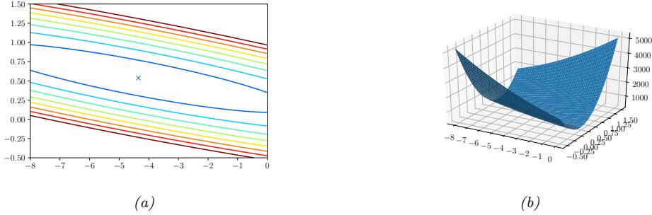
Figure 11.2: (a) Contours of the RSS error surface for the example in Figure 11.1a. The blue cross represents the MLE. (b) Corresponding surface plot. Generated by linreg\_contours\_sse\_plot.ipynb.

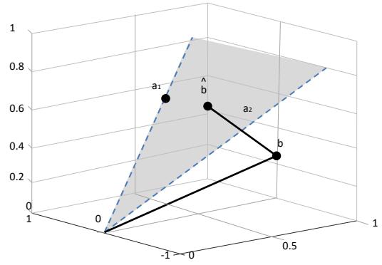
Figure 11.3: Graphical interpretation of least squares for m = 3 equations and n = 2 unknowns when solving the system Ax = b. a¹ and a² are the columns of A, which define a 2d linear subspace embedded in R³. The target vector b is a vector in R³; its orthogonal projection onto the linear subspace is denoted bˆ. The line from b to bˆ is the vector of residual errors, whose norm we want to minimize.

as an overdetermined system.) We seek a vector ^{yˆ → RN} that lies in the linear subspace spanned by X and is as close as possible to y, i.e., we want to find

\[\underset{\hat{\mathbf{y}}\in\text{span}(\{\mathfrak{x}\_{:,1},\ldots,\mathfrak{x}\_{:,d}\})}{\text{argmin}}\|\mathbf{y}-\hat{\mathbf{y}}\|\_{2}.\tag{11.12}\]

where x:,d is the d’th column of X. Since yˆ → span(X), there exists some weight vector w such that

\[ \hat{\mathbf{y}} = w\_1 \mathbf{x}\_{:,1} + \dots + w\_D \mathbf{x}\_{:,D} = \mathbf{X} \mathbf{w} \tag{11.13} \]

To minimize the norm of the residual, y ↑ yˆ, we want the residual vector to be orthogonal to every column of X. Hence

\[\mathbf{x}\_{:,d}^{\mathsf{T}}(\boldsymbol{y} - \boldsymbol{\hat{y}}) = \boldsymbol{0} \Rightarrow \mathbf{X}^{\mathsf{T}}(\boldsymbol{y} - \mathbf{X}\boldsymbol{w}) = \mathbf{0} \Rightarrow \boldsymbol{w} = (\mathbf{X}^{\mathsf{T}}\mathbf{X})^{-1}\mathbf{X}^{\mathsf{T}}\boldsymbol{y} \tag{11.14}\]

Hence our projected value of y is given by

\[ \hat{y} = \mathbf{X}w = \mathbf{X}(\mathbf{X}^\top \mathbf{X})^{-1}\mathbf{X}^\top y \tag{11.15} \]

This corresponds to an orthogonal projection of y onto the column space of X. For example, consider the case where we have N = 3 training examples, each of dimensionality D = 2. The training data defines a 2d linear subspace, defined by the 2 columns of X, each of which is a point in 3d. We project y, which is also a point in 3d, onto this 2d subspace, as shown in Figure 11.3.

The projection matrix

\[\text{Proj}(\mathbf{X}) \triangleq \mathbf{X}(\mathbf{X}^{\mathsf{T}}\mathbf{X})^{-1}\mathbf{X}^{\mathsf{T}} \tag{11.16}\]

is sometimes called the hat matrix, since yˆ = Proj(X)y. In the special case that X = x is a column vector, the orthogonal projection of y onto the line x becomes

\[\text{Proj}(x)y = x \frac{x^{\top}y}{x^{\top}x} \tag{11.17}\]

11.2.2.3 Algorithmic issues

Recall that the OLS solution is

\[ \hat{w} = \mathbf{X}^{\dagger}y = (\mathbf{X}^{\dagger}\mathbf{X})^{-1}\mathbf{X}^{\dagger}y\tag{11.18} \]

However, even if it is theoretically possible to compute the pseudo-inverse by inverting X^TX, we should not do so for numerical reasons, since X^TX may be ill conditioned or singular.

A better (and more general) approach is to compute the pseudo-inverse using the SVD. Indeed, if you look at the source code for the function sklearn.linear\_model.fit, you will see that it uses the scipy.linalg.lstsq function, which in turns calls DGELSD, which is an SVD-based solver implemented by the LAPACK library, written in Fortran.1

However, if X is tall and skinny (i.e., N ⇐ D), it can be quicker to use QR decomposition (Section 7.6.2). To do this, let X = QR, where Q^TQ = I. In Section 7.7, we show that OLS is equivalent to solving the system of linear equations X^w = ^y in a way that minimizes ||X^{w ↑ y}||² 2. (If N = D and X is full rank, the equations have a unique solution, and the error will be 0.) Using QR decomposition, we can rewrite this system of equations as follows:

\[(\mathbf{QR})w = y\tag{11.19}\]

\[\mathbf{Q}^{\mathsf{T}} \mathbf{Q} \mathbf{R} w = \mathbf{Q}^{\mathsf{T}} y\]

\[w = \mathbf{R}^{-1}(\mathbf{Q}^{\mathsf{T}}y) \tag{11.21}\]

Since R is upper triangular, we can solve this last set of equations using backsubstitution, thus avoiding matrix inversion. See linsys\_solve\_demo.ipynb for a demo.

An alternative to the use of direct methods based on matrix decomposition (such as SVD and QR) is to use iterative solvers, such as the conjugate gradient method (which assumes X is symmetric

^1. Note that a lot of the “Python” scientific computing stack sits on top of source code that is written in Fortran or C++, for reasons of speed. This makes it hard to change the underlying algorithms. By contrast, the scientific computing libraries in the Julia language are written in Julia itself, aiding clarity without sacrificing speed.

positive definite), and the GMRES (generalized minimal residual method), that works for general X. (In SciPy, this is implemented by sparse.linalg.gmres.) These methods just require the ability to perform matrix-vector multiplications (i.e., an implementation of a linear operator), and thus are well-suited to problems where X is sparse or structured. For details, see e.g., [TB97].

A final important issue is that it is usually essential to standardize the input features before fitting the model, to ensure that they are zero mean and unit variance. We can do this using Equation (10.51).

11.2.2.4 Weighted least squares

In some cases, we want to associate a weight with each example. For example, in heteroskedastic regression, the variance depends on the input, so the model has the form

\[p(y|\mathbf{z};\boldsymbol{\theta}) = \mathcal{N}(y|\mathbf{w}^{\mathsf{T}}\boldsymbol{x}, \sigma^{2}(\boldsymbol{x})) = \frac{1}{\sqrt{2\pi\sigma^{2}(\boldsymbol{x})}} \exp\left(-\frac{1}{2\sigma^{2}(\boldsymbol{x})}(y - \boldsymbol{w}^{\mathsf{T}}\boldsymbol{x})^{2}\right) \tag{11.22}\]

Thus

\[p(y|x; \theta) = \mathcal{N}(y|\mathbf{X}w, \Lambda^{-1})\tag{11.23}\]

where ” = diag(1/ε²(xn)). This is known as weighted linear regression. One can show that the MLE is given by

\[ \hat{w} = (\mathbf{X}^{\mathsf{T}} \mathbf{A} \mathbf{X})^{-1} \mathbf{X}^{\mathsf{T}} \Lambda y \tag{11.24} \]

This is known as the weighted least squares estimate.

11.2.3 Other approaches to computing the MLE

In this section, we discuss other approaches for computing the MLE.

11.2.3.1 Solving for o”set and slope separately

Typically we use a model of the form ^p(y|x, ^ω) = ^N (y|w^{0 + wT}x, ^ε2), where ^w0 is an o!set or “bias” term. We can compute (w0, w) at the same time by adding a column of 1s to X, and the computing the MLE as above. Alternatively, we can solve for w and w⁰ separately. (This will be useful later.) In particular, one can show that

\[ \hat{\boldsymbol{w}} = (\mathbf{X}\_c^\mathsf{T} \mathbf{X}\_c)^{-1} \mathbf{X}\_c^\mathsf{T} \mathbf{y}\_c = \left[ \sum\_{i=1}^N (\mathbf{x}\_n - \overline{\mathbf{x}})(\mathbf{x}\_n - \overline{\mathbf{x}})^\mathsf{T} \right]^{-1} \left[ \sum\_{i=1}^N (y\_n - \overline{y})(x\_n - \overline{x}) \right] \tag{11.25} \]

\[ \hat{w}\_0 = \frac{1}{N} \sum\_n y\_n - \frac{1}{N} \sum\_n \mathbf{x}\_n^\top \hat{w} = \overline{y} - \overline{\mathbf{z}}^T \hat{w} \tag{11.26} \]

where X^c is the centered input matrix containing x^{c n} = xⁿ ↑ x along its rows, and y^c = y ↑ y is the centered output vector. Thus we can first compute wˆ on centered data, and then estimate w⁰ using ^{y ↑ xT}w^ˆ .

Note that, if we write the model in the form ^{yˆ = 10 + εT}(^{x ↑ x}), then we have ^{εˆ = wˆ} and ^wˆ^{0 = 1}ˆ^{0 ↑ ε}ˆ^Tx, so ¹ˆ^{0 = y}.

11.2.3.2 Simple linear regression (1d inputs)

In the case of 1d (scalar) inputs, the results from Section 11.2.3.1 reduce to the following simple form, which may be familiar from basic statistics classes:

\[ \hat{w}\_1 = \frac{\sum\_n (x\_n - \overline{x})(y\_n - \bar{y})}{\sum\_n (x\_n - \bar{x})^2} = \frac{C\_{xy}}{C\_{xx}} = \rho\_{xy} \frac{\sigma\_y}{\sigma\_x} \tag{11.27} \]

\[ \hat{w}\_0 = \mathbb{E}\left[y\right] - w\_1 \mathbb{E}\left[x\right] \approx \bar{y} - \hat{w}\_1 \bar{x} \tag{11.28} \]

where Cxx = Cov [X, X] = V [X] = ε^{2 x}, Cyy = Cov [Y,Y ] = V [Y ] = ε^{2 y}, Cxy = Cov [X, Y ], and ςxy = ^Cxy ^εxε^y . Hence the prediction becomes yˆ = y¯ ↑ wˆ1x¯ + wˆ1x = y¯ = ςε^y (x→x¯) ^εy . We can interpret this equation as follows: we estimate how many standard deviations x is away from the mean of X, and then we predict the outcome to be the mean of Y plus ς times that many standard deviations above or below.

11.2.3.3 Partial regression

From Equation (11.27), we can compute the regression coe!cient of Y on X as follows:

\[R\_{YX} \triangleq \frac{\partial}{\partial x} \mathbb{E}\left[Y|X=x\right] = w\_1 = \frac{C\_{xy}}{C\_{xx}} \tag{11.29}\]

This is the slope of the linear prediction for Y given X.

Now consider the case where we have 2 inputs, so Y = w⁰ + w1X¹ + w2X² + ▷, where E [▷] = 0. One can show that the optimal regression coe”cient for w¹ is given by RY X1·X² , which is the partial regression coe!cient of Y on X1, keeping X² constant:

\[\text{for } w\_1 = R\_{YX\_1 \cdot X\_2} = \frac{\partial}{\partial x} \mathbb{E}\left[Y|X\_1 = x, X\_2\right] \tag{11.30}\]

Note that this quantity is invariant to the specific value of X² we condition on.

We can derive w² in a similar manner. Indeed, we can extend this to multiple input variables. In each case, we find the optimal coe”cients are equal to the partial regression coe”cients. This means that we can interpret the j’th coe”cient wˆ^j as the change in output y we expect per unit change in input x^j , keeping all the other inputs constant.

11.2.3.4 Recursively computing the MLE

OLS is a batch method for computing the MLE. In some applications, the data arrives in a continual stream, so we want to compute the estimate online, or recursively, as we discussed in Section 4.4.2. In this section, we show how to do this for the case of simple (1d) linear regession.

Recall from Section 11.2.3.2 that the batch MLE for simple linear regression is given by

\[ \hat{w}\_1 = \frac{\sum\_n (x\_n - \overline{x})(y\_n - \bar{y})}{\sum\_n (x\_n - \bar{x})^2} = \frac{C\_{xy}}{C\_{xx}} \tag{11.31} \]

\[ \hat{w}\_0 = \bar{y} - \hat{w}\_1 \bar{x} \tag{11.32} \]

where Cxy = Cov [X, Y ] and Cxx = Cov [X, X] = V [X].

We now discuss how to compute these results in a recursive fashion. To do this, let us define the following su”cient statistics:

\[\overline{x}^{(n)} = \frac{1}{n} \sum\_{i=1}^{n} x\_i, \quad \overline{y}^{(n)} = \frac{1}{n} \sum\_{i=1}^{n} y\_i \tag{11.33}\]

\[C\_{xx}^{(n)} = \frac{1}{n} \sum\_{i=1}^{n} (x\_i - \overline{x})^2, \quad C\_{xy}^{(n)} = \frac{1}{n} \sum\_{i=1}^{n} (x\_i - \overline{x})(y\_i - \overline{y}), \quad C\_{yy}^{(n)} = \frac{1}{n} \sum\_{i=1}^{n} (y\_i - \overline{y})^2 \tag{11.34}\]

We can update the means online using

\[ \overline{x}^{(n+1)} = \overline{x}^{(n)} + \frac{1}{n+1} (x\_{n+1} - \overline{x}^{(n)}), \quad \overline{y}^{(n+1)} = \overline{y}^{(n)} + \frac{1}{n+1} (y\_{n+1} - \overline{y}^{(n)}) \tag{11.35} \]

To update the covariance terms, let us first rewrite C(n) xy as follows:

\[C\_{xy}^{(n)} = \frac{1}{n} \left[ (\sum\_{i=1}^{n} x\_i y\_i) + (\sum\_{i=1}^{n} \overline{x}^{(n)} \overline{y}^{(n)}) - \overline{x}^{(n)} (\sum\_{i=1}^{n} y\_i) - \overline{y}^{(n)} (\sum\_{i=1}^{n} x\_i) \right] \tag{11.36}\]

\[=\frac{1}{n}\left[ (\sum\_{i=1}^{n} x\_i y\_i) + n\overline{x}^{(n)}\overline{y}^{(n)} - \overline{x}^{(n)} n\overline{y}^{(n)} - \overline{y}^{(n)} n\overline{x}^{(n)} \right] \tag{11.37}\]

\[\tilde{\lambda} = \frac{1}{n} \left[ (\sum\_{i=1}^{n} x\_i y\_i) - n \overline{x}^{(n)} \overline{y}^{(n)} \right] \tag{11.38}\]

Hence

\[\sum\_{i=1}^{n} x\_i y\_i = nC\_{xy}^{(n)} + n\overline{x}^{(n)}\overline{y}^{(n)}\tag{11.39}\]

and so

\[C\_{xy}^{(n+1)} = \frac{1}{n+1} \left[ x\_{n+1} y\_{n+1} + n C\_{xy}^{(n)} + n \overline{x}^{(n)} \overline{y}^{(n)} - (n+1) \overline{x}^{(n+1)} \overline{y}^{(n+1)} \right] \tag{11.40}\]

We can derive the update for C(n+1) xx in a similar manner.

See Figure 11.4 for a simple illustration of these equations in action for a 1d regression model.

To extend the above analysis to D-dimensional inputs, the easiest approach is to use SGD. The resulting algorithm is called the least mean squares algorithm; see Section 8.4.2 for details.

11.2.3.5 Deriving the MLE from a generative perspective

Linear regression is a discriminative model of the form p(y|x). However, we can also use generative models for regression, by analogy to how we use generative models for classification in Chapter 9, The goal is to compute the conditional expectation

\[f(\mathbf{z}) = \mathbb{E}\left[y|\mathbf{z}\right] = \int y \, p(y|\mathbf{z}) dy = \frac{\int y \, p(\mathbf{z}, y) dy}{\int p(\mathbf{z}, y) dy} \tag{11.41}\]

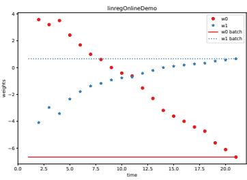
Figure 11.4: Regression coe”cients over time for the 1d model in Figure 1.7a(a). Generated by linregOnlineDemo.ipynb.

Suppose we fit p(x, y) using an MVN. The MLEs for the parameters of the joint distribution are the empiricial means and covariances (see Section 4.2.6 for a proof of this result):

\[ \mu\_x = \frac{1}{N} \sum\_n x\_n \tag{11.42} \]

\[ \mu\_y = \frac{1}{N} \sum\_n y\_n \tag{11.43} \]

\[\Delta \Sigma\_{xx} = \frac{1}{N} \sum\_{n} (x\_n - \overline{x})(x\_n - \overline{x})^\top = \frac{1}{N} \mathbf{X}\_c^\top \mathbf{X}\_c \tag{11.44}\]

\[\Delta \Sigma\_{xy} = \frac{1}{N} \sum\_{n} (x\_n - \overline{x})(y\_n - \overline{y}) = \frac{1}{N} \mathbf{X}\_c^\top y\_c \tag{11.45}\]

Hence from Equation (3.28), we have

\[\mathbb{E}\left[y|x\right] = \mu\_y + \Sigma\_{xy}^{\mathsf{T}} \Sigma\_{xx}^{-1} (x - \mu\_x) \tag{11.46}\]

We can rewrite this as ^E [y|x] = ^{w0 + wTx} by defining

\[w\_0 = \mu\_y - w^\mathsf{T}\mu\_x = \overline{y} - w^\mathsf{T}\overline{x} \tag{11.47}\]

\[\mathbf{w} = \boldsymbol{\Sigma}\_{xx}^{-1} \boldsymbol{\Sigma}\_{xy} = \left(\mathbf{X}\_c^{\mathsf{T}} \mathbf{X}\_c\right)^{-1} \mathbf{X}\_c^{\mathsf{T}} y\_c \tag{11.48}\]

This matches the MLEs for the discriminative model as we showed in Section 11.2.3.1. Thus we see that fitting the joint model, and then conditioning it, yields the same result as fitting the conditional model. However, this is only true for Gaussian models (see Section 9.4 for further discussion of this point).

11.2.3.6 Deriving the MLE for ⇀²

After estimating wˆ mle using one of the above methods, we can estimate the noise variance. It is easy to show that the MLE is given by

\[\hat{\sigma}\_{\text{mle}}^2 = \underset{\sigma^2}{\text{argmin}} \, \text{NLL}(\hat{w}, \sigma^2) = \frac{1}{N} \sum\_{n=1}^N (y\_n - \mathbf{z}\_n^\mathrm{T} \hat{w})^2 \tag{11.49}\]

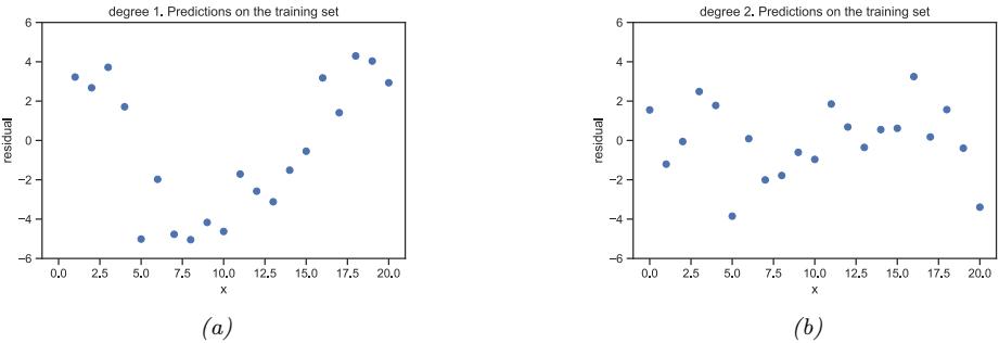
Figure 11.5: Residual plot for polynomial regression of degree 1 and 2 for the functions in Figure 1.7a(a-b). Generated by linreg\_poly\_vs\_degree.ipynb.

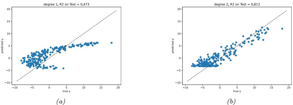
Figure 11.6: Fit vs actual plots for polynomial regression of degree 1 and 2 for the functions in Figure 1.7a(a-b). Generated by linreg\_poly\_vs\_degree.ipynb.

This is just the MSE of the residuals, which is an intuitive result.

11.2.4 Measuring goodness of fit

In this section, we discuss some simple ways to assess how well a regression model fits the data (which is known as goodness of fit).

11.2.4.1 Residual plots

For 1d inputs, we can check the reasonableness of the model by plotting the residuals, rⁿ = yⁿ ↑ yˆn, vs the input xn. This is called a residual plot. The model assumes that the residuals have a ^N (0, ^ε2) distribution, so the residual plot should be a cloud of points more or less equally above and below the horizontal line at 0, without any obvious trends.

As an example, in Figure 11.5(a), we plot the residuals for the linear model in Figure 1.7a(a). We see that there is some curved structure to the residuals, indicating a lack of fit. In Figure 11.5(b), we plot the residuals for the quadratic model in Figure 1.7a(b). We see a much better fit.

To extend this approach to multi-dimensional inputs, we can plot predictions yˆⁿ vs the true output yn, rather than plotting vs xn. A good model will have points that lie on a diagonal line. See Figure 11.6 for some examples.

11.2.4.2 Prediction accuracy and R²

We can assess the fit quantitatively by computing the RSS (residual sum of squares) on the dataset: RSS(w) = $^{N n}=1(y^{n ↑ wT}xn)2. A model with lower RSS fits the data better. Another measure that is used is root mean squared error or RMSE:

\[\text{RMSE}(\mathbf{w}) \triangleq \sqrt{\frac{1}{N} \text{RSS}(\mathbf{w})} \tag{11.50}\]

A more interpretable measure can be computed using the coe!cient of determination, denoted by R²:

\[R^2 \triangleq 1 - \frac{\sum\_{n=1}^{N} (\hat{y}\_n - y\_n)^2}{\sum\_{n=1}^{N} (\overline{y} - y\_n)^2} = 1 - \frac{\text{RSS}}{\text{TSS}} \tag{11.51}\]

where y = ¹ N $^{N n}=1 ^yn is the empirical mean of the response, RSS ⁼ $^{N n}=1(y^{n ↑ y}ˆn)² is the residual sum of squares, and TSS = $^{N n}=1(y^{n ↑}y)² is the total sum of squares. Thus we see that ^R2 measures the variance in the predictions relative to a simple constant prediction of yˆⁿ = y. If a model does no better at predicting than using the mean of the output, it we have R² = 0. If the model perfectly fits the data, then the RSS will be 0, so R² = 1. In general, larger values imply greater reduction in variance (better fit). This is illustrated in Figure 11.6.

11.3 Ridge regression

Maximum likelihood estimation can result in overfitting, as we discussed in Section 1.2.2.2. A simple solution to this is to use MAP estimation with a zero-mean Gaussian prior on the weights, ^p(w) = ^N (w|0, ^φ→¹I), as we discused in Section 4.5.3. This is called ridge regression.

In more detail, we compute the MAP estimate as follows:

\[ \hat{w}\_{\text{map}} = \operatorname\*{argmin} \frac{1}{2\sigma^2} (\mathbf{y} - \mathbf{X}w)^\top (\mathbf{y} - \mathbf{X}w) + \frac{1}{2\tau^2} w^\top w \tag{11.52} \]

\[\mathbf{w} = \operatorname\*{argmin}{\operatorname{RSS}}(\mathbf{w}) + \lambda ||\mathbf{w}||\_2^2 \tag{11.53}\]

where φ ↭ ^{ε2 ς2} is proportional to the strength of the prior, and

\[||\mathbf{w}||\_2 \triangleq \sqrt{\sum\_{d=1}^D |w\_d|^2} = \sqrt{\mathbf{w}^\mathsf{T}\mathbf{w}} \tag{11.54}\]

is the ω² norm of the vector w. Thus we are penalizing weights that become too large in magnitude. In general, this technique is called ω² regularization or weight decay, and is very widely used. See Figure 4.5 for an illustration.

Note that we do not penalize the o!set term w0, since that only a!ects the global mean of the output, and does not contribute to overfitting. See Exercise 11.2.

11.3.1 Computing the MAP estimate

In this section, we discuss algorithms for computing the MAP estimate.

The MAP estimate corresponds to minimizing the following penalized objective:

\[J(w) = (y - \mathbf{Xw})^{\mathsf{T}}(y - \mathbf{Xw}) + \lambda ||w||\_2^2 \tag{11.55}\]

where φ = ε²/τ ² is the strength of the regularizer. The derivative is given by

\[\nabla\_{\mathbf{w}} J(w) = 2\left(\mathbf{X}^{\mathsf{T}} \mathbf{X}w - \mathbf{X}^{\mathsf{T}}y + \lambda w\right) \tag{11.56}\]

and hence

\[\hat{w}\_{\text{map}} = (\mathbf{X}^{\mathsf{T}}\mathbf{X} + \lambda\mathbf{I}\_{D})^{-1}\mathbf{X}^{\mathsf{T}}\mathbf{y} = (\sum\_{n} x\_{n}\mathbf{z}\_{n}^{\mathsf{T}} + \lambda\mathbf{I}\_{D})^{-1}(\sum\_{n} y\_{n}\mathbf{z}\_{n}) \tag{11.57}\]

11.3.1.1 Solving using QR

Naively computing the primal estimate w = (XTX + φI)→1X^Ty using matrix inversion is a bad idea, since it can be slow and numerically unstable. In this section, we describe a way to convert the problem to a standard least squares problem, to which we can apply QR decomposition, as discussed in Section 11.2.2.3.

We assume the prior has the form ^p(w) = ^N (0, “^→1), where” is the precision matrix. In the case of ridge regression, ” = (1/τ ²)I. We can emulate this prior by adding “virtual data” to the training set to get

\[\tilde{\mathbf{X}} = \begin{pmatrix} \mathbf{X}/\sigma \\ \sqrt{\mathbf{A}} \end{pmatrix}, \quad \tilde{\mathbf{y}} = \begin{pmatrix} \mathbf{y}/\sigma \\ \mathbf{0}\_{D \times 1} \end{pmatrix} \tag{11.58}\]

where ” ^{= ≃} ” ≃ “^T is a Cholesky decomposition of”. We see that ^X˜ is (^{N + D}) ^{↓ D}, where the extra rows represent pseudo-data from the prior.

We now show that the RSS on this expanded data is equivalent to penalized RSS on the original data:

\[f(w) = (\ddot{y} - \ddot{\mathbf{X}}w)^{\sf T}(\ddot{y} - \ddot{\mathbf{X}}w) \tag{11.59}\]

\[\mathbf{x} = \left( \begin{pmatrix} \mathbf{y}/\sigma \\ \mathbf{0} \end{pmatrix} - \begin{pmatrix} \mathbf{X}/\sigma \\ \sqrt{\mathbf{A}} \end{pmatrix} w \right)^{\top} \left( \begin{pmatrix} \mathbf{y}/\sigma \\ \mathbf{0} \end{pmatrix} - \begin{pmatrix} \mathbf{X}/\sigma \\ \sqrt{\mathbf{A}} \end{pmatrix} w \right) \tag{11.60}\] \(\mathbf{x} \in \mathbb{R}^{N \times N} \text{ and } \mathbf{y} \in \mathbb{R}^{N \times N}\)

\[\mathbf{x} = \begin{pmatrix} \frac{1}{\sigma}(\mathbf{y} - \mathbf{X}\mathbf{w}) \\ -\sqrt{\mathbf{A}}\mathbf{w} \end{pmatrix}^{\mathsf{T}} \begin{pmatrix} \frac{1}{\sigma}(\mathbf{y} - \mathbf{X}\mathbf{w}) \\ -\sqrt{\mathbf{A}}\mathbf{w} \end{pmatrix} \tag{11.61}\]

\[\mathbf{x} = \frac{1}{\sigma^2} (\mathbf{y} - \mathbf{X}w)^\mathsf{T} (\mathbf{y} - \mathbf{X}w) + (\sqrt{\Lambda}w)^\mathsf{T} (\sqrt{\Lambda}w) \tag{11.62}\]

\[\mathbf{y} = \frac{1}{\sigma^2} (\mathbf{y} - \mathbf{X}\,\mathbf{w})^\mathsf{T} (\mathbf{y} - \mathbf{X}\,\mathbf{w}) + \mathbf{w}^\mathsf{T} \boldsymbol{\Lambda}\mathbf{w} \tag{11.63}\]

Hence the MAP estimate is given by

\[ \hat{w}\_{\text{map}} = (\bar{\mathbf{X}}^{\text{T}} \bar{\mathbf{X}})^{-1} \bar{\mathbf{X}}^{\text{T}} \tilde{y} \tag{11.64} \]

which can be solved using standard OLS methods. In particular, we can compute the QR decomposition of X˜ , and then proceed as in Section 11.2.2.3. This takes O((N + D)D²) time.

11.3.1.2 Solving using SVD

In this section, we assume D>N, which is the usual case when using ridge regression. In this case, it is faster to use SVD than QR. To see how this works, let X = USV^T be the SVD of X, where ^VT^{V = IN} , UU^{T = U}T^{U = IN} , and ^S is a diagonal ^{N ↓ N} matrix. Now let ^{R =} US be an ^{N ↓ N} matrix. One can show (see Exercise 18.4 of [HTF09]) that

\[ \hat{w}\_{\text{map}} = \mathbf{V}(\mathbf{R}^{\mathsf{T}}\mathbf{R} + \lambda \mathbf{I}\_N)^{-1} \mathbf{R}^{\mathsf{T}} \mathbf{y} \tag{11.65} \]

In other words, we can replace the D-dimensional vectors xⁱ with the N-dimensional vectors rⁱ and perform our penalized fit as before. The overall time is now O(DN²) operations, which is less than O(D³) if D>N.

11.3.2 Connection between ridge regression and PCA

In this section, we discuss an interesting connection between ridge regression and PCA (which we describe in Section 20.1), in order to gain further insight into why ridge regression works well. Our discussion is based on [HTF09, p66].

Let X = USV^T be the SVD of X, where V^TV = I^N , UU^T = U^TU = I^N , and S is a diagonal N ↓ N matrix. Using Equation (11.65) we can see that the ridge predictions on the training set are given by

\[ \hat{y} = \mathbf{X}\hat{w}\_{\text{map}} = \mathbf{U}\mathbf{S}\mathbf{V}^{\text{T}}\mathbf{V}(\mathbf{S}^2 + \lambda\mathbf{I})^{-1}\mathbf{S}\mathbf{U}^{\text{T}}\mathbf{y} \tag{11.66} \]

\[\mathbf{y} = \mathbf{U}\mathbf{\bar{S}}\mathbf{U}^{\mathsf{T}}\mathbf{y} = \sum\_{j=1}^{D} \mathbf{u}\_{j}\mathbf{\bar{S}}\_{jj}\mathbf{u}\_{j}^{\mathsf{T}}\mathbf{y} \tag{11.67}\]

where

\[\tilde{S}\_{jj} \triangleq [\mathbf{S}(\mathbf{S}^2 + \lambda I)^{-1}\mathbf{S}]\_{jj} = \frac{\sigma\_j^2}{\sigma\_j^2 + \lambda} \tag{11.68}\]

and ε^j are the singular values of X. Hence

\[\hat{\mathbf{y}} = \mathbf{X}\hat{\boldsymbol{w}}\_{\text{map}} = \sum\_{j=1}^{D} \boldsymbol{u}\_{j} \frac{\sigma\_{j}^{2}}{\sigma\_{j}^{2} + \lambda} \boldsymbol{u}\_{j}^{\text{T}} \mathbf{y} \tag{11.69}\]

In contrast, the least squares prediction is

\[\hat{\boldsymbol{\omega}} \cdot \hat{\boldsymbol{y}} = \mathbf{X} \hat{\boldsymbol{w}}\_{\text{mle}} = (\mathbf{U} \mathbf{S} \mathbf{V}^{\text{T}}) (\mathbf{V} \mathbf{S}^{-1} \mathbf{U}^{\text{T}} \mathbf{y}) = \mathbf{U} \mathbf{U}^{\text{T}} \mathbf{y} = \sum\_{j=1}^{D} u\_{j} u\_{j}^{\text{T}} \mathbf{y} \tag{11.70}\]

If ε^{2 j} is large compared to φ, then ε^{2 j} /(ε^{2 j} + ^φ) ↖ ^{ε2 j} /ε^{2 j} = 1, so direction u^j is not a!ected, but if ε2 ^j is small compared to φ, and if φ is large, then ε^{2 j} /(ε^{2 j} + φ) ↖ 1/φ ↖ 0, so direction u^j will be downweighted. In view of this, we define the e!ective number of degrees of freedom of the model as follows:

\[\text{dof}(\lambda) = \sum\_{j=1}^{D} \frac{\sigma\_j^2}{\sigma\_j^2 + \lambda} \tag{11.71}\]

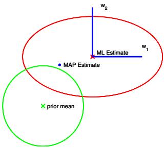
Figure 11.7: Geometry of ridge regression. The likelihood is shown as an ellipse, and the prior is shown as a circle centered on the origin. Adapted from Figure 3.15 of [Bis06]. Generated by geom\_ridge.ipynb.

When φ = 0, dof(φ) = D, and as φ ↔︎ ∈, dof(φ) ↔︎ 0.

Let us try to understand why this behavior is desirable. In Section 11.7, we show that Cov [w|D] ∞ (X^TX)→¹, if we use a uniform prior for w. Thus the directions in which we are most uncertain about w are determined by the eigenvectors of (X^TX)→¹ with the largest eigenvalues, as shown in Figure 7.6. These drections correspond to the eigenvectors of X^TX with the smallest eigenvalues, and hence (from Section 7.5.2) the smallest singular values. So if ε^{2 j} is small relative to φ, ridge regression will downweight direction u^j .

This process is illustrated in Figure 11.7. The horizontal w¹ parameter is not-well determined by the data (has high posterior variance), but the vertical w² parameter is well-determined. Hence wmap(2) is close to wmle(2), but wmap(1) is shifted strongly towards the prior mean, which is 0. In this way, ill-determined parameters are reduced in size towards 0. This is called shrinkage.

There is a related, but di!erent, technique called principal components regression, which is a supervised version of PCA, which we explain in Section 20.1. The idea is this: first use PCA to reduce the dimensionality to K dimensions, and then use these low dimensional features as input to regression. However, this technique does not work as well as ridge regression in terms of predictive accuracy [HTF01, p70]. The reason is that in PC regression, only the first K (derived) dimensions are retained, and the remaining D ↑ K dimensions are entirely ignored. By contrast, ridge regression uses a “soft” weighting of all the dimensions.

11.3.3 Choosing the strength of the regularizer

To find the optimal value of φ, we can try a finite number of distinct values, and use cross validation to estimate their expected loss, as discussed in Section 4.5.5.2. See Figure 4.5d for an example.

This approach can be quite expensive if we have many values to choose from. Fortunately, we can often warm start the optimization procedure, using the value of wˆ (φk) as an initializer for wˆ (φk+1), where φk+1 < φk; in other words, we start with a highly constrained model (strong regularizer), and then gradually relax the constraints (decrease the amount of regularization). The set of parameters wˆ ^k that we sweep out in this way is known as the regularization path. See Figure 11.10(a) for an example.

We can also use an empirical Bayes approach to choose φ. In particular, we choose the hyperparameter by computing ^{φˆ =} argmax↼ log ^p(D|φ), where ^p(D|φ) is the marginal likelihood or evidence.

Figure 4.7b shows that this gives essentially the same result as the CV estimate. However, the Bayesian approach has several advantages: computing p(D|φ) can be done by fitting a single model, whereas CV has to fit the same model K times; and p(D|φ) is a smooth function of φ, so we can use gradient-based optimization instead of discrete search.

11.4 Lasso regression

In Section 11.3, we assumed a Gaussian prior for the regression coe”cients when fitting linear regression models. This is often a good choice, since it encourages the parameters to be small, and hence prevents overfitting. However, sometimes we want the parameters to not just be small, but to be exactly zero, i.e., we want wˆ to be sparse, so that we minimize the L0-norm:

\[||\mathbf{w}||\_0 = \sum\_{d=1}^{D} \mathbb{I}\left(|w\_d| > 0\right) \tag{11.72}\]

This is useful because it can be used to perform feature selection. To see this, note that the prediction has the form f(x; w) = $^{D d}=1 wdxd, so if any w^d = 0, we ignore the corresponding feature xd. (The same idea can be applied to nonlinear models, such as DNNs, by encouraging the first layer weights to be sparse.)

11.4.1 MAP estimation with a Laplace prior (▷¹ regularization)

There are many ways to compute such sparse estimates (see e.g., [Bha+19]). In this section we focus on MAP estimation using the Laplace distribution (which we discussed in Section 11.6.1) as the prior:

\[p(w|\lambda) = \prod\_{d=1}^{D} \text{Laplace}(w\_d|0, 1/\lambda) \propto \prod\_{d=1}^{D} e^{-\lambda|w\_d|} \tag{11.73}\]

where φ is the sparsity parameter, and

\[\text{Laplace}(w|\mu, b) \stackrel{\Delta}{=} \frac{1}{2b} \exp\left(-\frac{|w - \mu|}{b}\right) \tag{11.74}\]

Here µ is a location parameter and b > 0 is a scale parameter. Figure 2.15 shows that Laplace(w|0, b) puts more density on 0 than ^N (w|0, ^ε2), even when we fix the variance to be the same.

To perform MAP estimation of a linear regression model with this prior, we just have to minimize the following objective:

\[\text{PNLLL}(w) = -\log p(\mathcal{D}|w) - \log p(w|\lambda) = ||\mathbf{X}w - \mathbf{y}||\_2^2 + \lambda ||w||\_1 \tag{11.75}\]

where ||w||¹ ↭ $^{D d}=1 |wd| is the ω¹ norm of w. This method is called lasso, which stands for “least absolute shrinkage and selection operator” [Tib96]. (We explain the reason for this name below.) More generally, MAP estimation with a Laplace prior is called ω1-regularization.

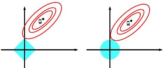
Figure 11.8: Illustration of ,¹ (left) vs ,² (right) regularization of a least squares problem. Adapted from Figure 3.12 of [HTF01].

Note also that we could use other norms for the weight vector. In general, the q-norm is defined as follows:

\[\|\|w\|\|\_{q} = \left(\sum\_{d=1}^{D} |w\_d|^q\right)^{1/q} \tag{11.76}\]

For q < 1, we can get even sparser solutions. In the limit where q = 0, we get the ω0-norm:

\[\|\|w\|\|\_{0} = \sum\_{d=1}^{D} \mathbb{I}\left(|w\_d| > 0\right) \tag{11.77}\]

However, one can show that for any q < 1, the problem becomes non-convex (see e.g., [HTW15]). Thus ω1-norm is the tightest convex relaxation of the ω0-norm.

11.4.2 Why does ▷¹ regularization yield sparse solutions?

We now explain why ω¹ regularization results in sparse solutions, whereas ω² regularization does not. We focus on the case of linear regression, although similar arguments hold for other models.

The lasso objective is the following non-smooth objective (see Section 8.1.4 for a discussion of smoothness):

\[\min\_{\mathbf{w}} \text{NLL}(\mathbf{w}) + \lambda ||\mathbf{w}||\_1 \tag{11.78}\]

This is the Lagrangian for the following quadratic program (see Section 8.5.4):

\[\min\_{\mathbf{w}} \text{NLL}(\mathbf{w}) \quad \text{s.t.} \quad ||\mathbf{w}||\_1 \le B \tag{11.79}\]

where B is an upper bound on the ω1-norm of the weights: a small (tight) bound B corresponds to a large penalty φ, and vice versa.

Similarly, we can write the ridge regression objective min^w NLL(w) + ^φ||w||^{2 2} in bound constrained form:

\[\min\_{\mathbf{w}} \text{NLL}(\mathbf{w}) \quad \text{s.t.} \quad ||\mathbf{w}||\_2^2 \le B \tag{11.80}\]

In Figure 11.8, we plot the contours of the NLL objective function, as well as the contours of the ω² and ω¹ constraint surfaces. From the theory of constrained optimization (Section 8.5) we know that the optimal solution occurs at the point where the lowest level set of the objective function intersects the constraint surface (assuming the constraint is active). It should be geometrically clear that as we relax the constraint B, we “grow” the ω¹ “ball” until it meets the objective; the corners of the ball are more likely to intersect the ellipse than one of the sides, especially in high dimensions, because the corners “stick out” more. The corners correspond to sparse solutions, which lie on the coordinate axes. By contrast, when we grow the ω² ball, it can intersect the objective at any point; there are no “corners”, so there is no preference for sparsity.

11.4.3 Hard vs soft thresholding

The lasso objective has the form L(w) = NLL(w) + φ||w||1. One can show (Exercise 11.3) that the gradient for the smooth NLL part is given by

\[\frac{\partial}{\partial w\_d} \text{NLL}(w) = a\_d w\_d - c\_d \tag{11.81}\]

\[a\_d = \sum\_{n=1}^{N} x\_{nd}^2\tag{11.82}\]

\[\mathbf{c}\_d = \sum\_{n=1}^{N} x\_{nd} (y\_n - \mathbf{w}\_{-d}^\mathsf{T} \mathbf{x}\_{n,-d}) \tag{11.83}\]

where w→^d is w without component d, and similarly xn,→^d is feature vector xⁿ without component d. We see that c^d is proportional to the correlation between d’th column of features, x:,d, and the residual error obtained by predicting using all the other features, r→^d = y ↑ X:,→^dw→^d. Hence the magnitude of c^d is an indication of how relevant feature d is for predicting y, relative to the other features and the current parameters. Setting the gradient to 0 gives the optimal update for wd, keeping all other weights fixed:

\[w\_d = c\_d / a\_d = \frac{x\_{:,d}^\uparrow r\_{-d}}{||x\_{:,d}||\_2^2} \tag{11.84}\]

The corresponding new prediction for r→^d becomes rˆ→^d = wdx:,d, which is the orthogonal projection of the residual onto the column vector x:,d, consistent with Equation (11.15).

Now we add in the ω¹ term. Unfortunately, the ||w||¹ term is not di!erentiable whenever w^d = 0. Fortunately, we can still compute a subgradient at this point. Using Equation (8.14) we find that

\[\partial\_{w\_d} \mathcal{L}(\mathbf{w}) = (a\_d w\_d - c\_d) + \lambda \partial\_{w\_d} ||\mathbf{w}||\_1 \tag{11.85}\]

\[= \begin{cases} \begin{array}{l} \{a\_d w\_d - c\_d - \lambda\} & \text{if } w\_d < 0\\ \left[ -c\_d - \lambda, -c\_d + \lambda \right] & \text{if } w\_d = 0\\ \{a\_d w\_d - c\_d + \lambda\} & \text{if } w\_d > 0 \end{array} \tag{11.86}\]

Depending on the value of cd, the solution to 0^wd L(w)=0 can occur at 3 di!erent values of wd, as follows:

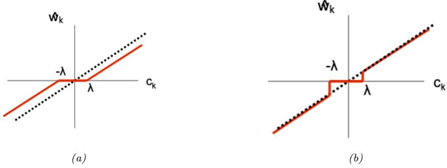
Figure 11.9: Left: soft thresholding. Right: hard thresholding. In both cases, the horizontal axis is the residual error incurred by making predictions using all the coe”cients except for wk, and the vertical axis is the estimated coe”cient wˆ^k that minimizes this penalized residual. The flat region in the middle is the interval [↑↼, +↼].

• 1. If c^d < ↑φ, so the feature is strongly negatively correlated with the residual, then the subgradient is zero at wˆ^d = ^cd+↼ ^ad < 0.
• 2. If c^d → [↑φ, φ], so the feature is only weakly correlated with the residual, then the subgradient is zero at wˆ^d = 0.
• 3. If c^d > φ, so the feature is strongly positively correlated with the residual, then the subgradient is zero at wˆ^d = ^cd→↼ ^ad > 0.

In summary, we have

\[\hat{w}\_d(c\_d) = \begin{cases} (c\_d + \lambda)/a\_d & \text{if } c\_d < -\lambda \\ 0 & \text{if } c\_d \in [-\lambda, \lambda] \\ (c\_d - \lambda)/a\_d & \text{if } c\_d > \lambda \end{cases} \tag{11.87}\]

We can write this as follows:

\[ \hat{w}\_d = \text{SoftThreshold}(\frac{c\_d}{a\_d}, \lambda/a\_d) \tag{11.88} \]

where

\[\text{SoftThreshold}(x, \delta) \stackrel{\Delta}{=} \text{sign}(x) \left( |x| - \delta \right)\_{+} \tag{11.89}\]

and x⁺ = max(x, 0) is the positive part of x. This is called soft thresholding (see also Section 8.6.2). This is illustrated in Figure 11.9(a), where we plot wˆ^d vs cd. The dotted black line is the line w^d = cd/a^d corresponding to the least squares fit. The solid red line, which represents the regularized estimate wˆd, shifts the dotted line down (or up) by φ, except when ↑φ ↘ c^d ↘ φ, in which case it sets w^d = 0.

By contrast, in Figure 11.9(b), we illustrate hard thresholding. This sets values of w^d to 0 if ↑φ ↘ c^d ↘ φ, but it does not shrink the values of w^d outside of this interval. The slope of the soft

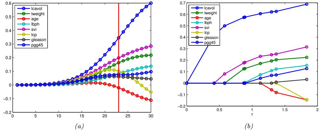
Figure 11.10: (a) Profiles of ridge coe”cients for the prostate cancer example vs bound B on ,² norm of w, so small B (large ↼) is on the left. The vertical line is the value chosen by 5-fold CV using the 1 standard error rule. Adapted from Figure 3.8 of [HTF09]. Generated by ridgePathProstate.ipynb. (b) Same as (a) but using ,¹ norm of w. The x-axis shows the critical values of ↼ = 1/B, where the regularization path is discontinuous. Adapted from Figure 3.10 of [HTF09]. Generated by lassoPathProstate.ipynb.

thresholding line does not coincide with the diagonal, which means that even large coe”cients are shrunk towards zero. This is why lasso stands for “least absolute selection and shrinkage operator”. Consequently, lasso is a biased estimator (see Section 4.7.6.1).

A simple solution to the biased estimate problem, known as debiasing, is to use a two-stage estimation process: we first estimate the support of the weight vector (i.e., identify which elements are non-zero) using lasso; we then re-estimate the chosen coe”cients using least squares. For an example of this in action, see Figure 11.13.

11.4.4 Regularization path

If φ = 0, we get the OLS solution. which will be dense. As we increase φ, the solution vector wˆ (φ) will tend to get sparser. If φ is bigger than some critical value, we get wˆ = 0. This critical value is obtained when the gradient of the NLL cancels out with the gradient of the penalty:

\[\lambda\_{\text{max}} = \max\_{d} |\nabla\_{\mathbf{w}\_d} \text{NLL}(\mathbf{0})| = \max\_{d} c\_d(\mathbf{w} = 0) = \max\_{d} |\mathbf{y}^{\mathsf{T}} \mathbf{z}\_{:,d}| = ||\mathbf{X}^{\mathsf{T}} \mathbf{y}||\_{\infty} \tag{11.90}\]

Alternatively, we can work with the bound B on the ω¹ norm. When B = 0, we get wˆ = 0. As we increase B, the solution becomes denser. The largest value of B for which any component is zero is given by Bmax = ||wˆ mle||1.

As we increase φ, the solution vector wˆ gets sparser, although not necessarily monotonically. We can plot the values wˆ^d vs φ (or vs the bound B) for each feature d; this is known as the regularization path. This is illustrated in Figure 11.10(b), where we apply lasso to the prostate cancer regression dataset from [HTF09]. (We treat features gleason and svi as numeric, not categorical.) On the left,

0	0	0	0	0	0	0	0
0	0	0	0	0	0	0	0.4279
0	0	0	0	0	0	0.0735	0.5015
0	0	0	0.0930	0	0	0.1878	0.5610
0	0	0	0.0963	0.0036	0	0.1890	0.5622
0.0901	0	0	0.2003	0.1435	0	0.2456	0.5797
0.1066	0	0	0.2082	0.1639	-0.0321	0.2572	0.5864
0.2452	0	-0.2565	0.3003	0.2062	-0.1337	0.2910	0.6994
0.2773	-0.0209	-0.2890	0.3096	0.2120	-0.1425	0.2926	0.7164

Table 11.1: Values of the coe”cients for linear regression model fit to prostate cancer dataset as we vary the strength of the ,¹ regularizer. These numbers are plotted in Figure 11.10(b).

when B = 0, all the coe”cients are zero. As we increase B, the coe”cients gradually “turn on”.2 The analogous result for ridge regression is shown in Figure 11.10(a). For ridge, we see all coe”cients are non-zero (assuming φ > 0), so the solution is not sparse.

Remarkably, it can be shown that the lasso solution path is a piecewise linear function of φ [Efr+04; GL15]. That is, there are a set of critical values of φ where the active set of non-zero coe”cients changes. For values of φ between these critical values, each non-zero coe”cient increases or decreases in a linear fashion. This is illustrated in Figure 11.10(b). Furthermore, one can solve for these critical values analytically [Efr+04]. In Table 11.1. we display the actual coe”cient values at each of these critical steps along the regularization path (the last line is the least squares solution).

By changing φ from φmax to 0, we can go from a solution in which all the weights are zero to a solution in which all weights are non-zero. Unfortunately, not all subset sizes are achievable using lasso. In particular, one can show that, if D>N, the optimal solution can have at most N variables in it, before reaching the complete set corresponding to the OLS solution of minimal ω¹ norm. In Section 11.4.8, we will see that by using an ω² regularizer as well as an ω¹ regularizer (a method known as the elastic net), we can achieve sparse solutions which contain more variables than training cases. This lets us explore model sizes between N and D.

11.4.5 Comparison of least squares, lasso, ridge and subset selection

In this section, we compare least squares, lasso, ridge and subset selection. For simplicity, we assume all the features of X are orthonormal, so X^TX = I. In this case, the NLL is given by

\[\text{NLL}(w) = ||\mathbf{y} - \mathbf{X}w||^2 = \mathbf{y}^\mathsf{T}\mathbf{y} + w^\mathsf{T}\mathbf{X}^\mathsf{T}\mathbf{X}w - 2w^\mathsf{T}\mathbf{X}^\mathsf{T}\mathbf{y} \tag{11.91}\]

\[=\text{const} + \sum\_{d} w\_d^2 - 2\sum\_{d} \sum\_{n} w\_d x\_{nd} y\_n \tag{11.92}\]

so we see this factorizes into a sum of terms, one per dimension. Hence we can write down the MAP and ML estimates analytically for each w^d separately, as given below.

• MLE From Equation (11.85), the OLS solution is given by

\[ \hat{w}\_d^{\text{mle}} = c\_d / a\_d = \mathbf{z}\_{:d}^{\text{T}} \mathbf{y} \tag{11.93} \]

where x:^d is the d’th column of X.

^2. It is common to plot the solution versus the shrinkage factor, defined as s(B) = B/Bmax, rather than against B. This merely a!ects the scale of the horizontal axis, not the shape of the curves.

Term	OLS	Best Subset	Ridge	Lasso
intercept	2.465	2.477	2.467	2.465
lcalvol	0.676	0.736	0.522	0.548
lweight	0.262	0.315	0.255	0.224
age	-0.141	0.000	-0.089	0.000
lbph	0.209	0.000	0.186	0.129
svi	0.304	0.000	0.259	0.186
lcp	-0.287	0.000	-0.095	0.000
gleason	-0.021	0.000	0.025	0.000
pgg45	0.266	0.000	0.169	0.083
Test error	0.521	0.492	0.487	0.457
Std error	0.176	0.141	0.157	0.146

Figure 11.11: Results of di!erent methods on the prostate cancer data, which has 8 features and 67 training cases. Methods are: OLS = ordinary least squares, Subset = best subset regression, Ridge, Lasso. Rows represent the coe”cients; we see that subset regression and lasso give sparse solutions. Bottom row is the mean squared error on the test set (30 cases). Adapted from Table 3.3. of [HTF09]. Generated by prostate\_comparison.ipynb.

• Ridge One can show that the ridge estimate is given by

\[ \hat{w}\_d^{\text{ridge}} = \frac{\hat{w}\_d^{\text{mle}}}{1 + \lambda} \tag{11.94} \]

• Lasso From Equation (11.88), and using the fact that wˆmle ^d = cd/ad, we have

\[\hat{w}\_d^{\text{lasso}} = \text{sign}(\hat{w}\_d^{\text{mle}}) \left( |\hat{w}\_d^{\text{mle}}| - \lambda \right)\_+ \tag{11.95}\]

This corresponds to soft thresholding, shown in Figure 11.9(a).

• Subset selection If we pick the best K features using subset selection, the parameter estimate is as follows

\[ \hat{w}\_d^{\rm ss} = \begin{cases} \hat{w}\_d^{\rm mle} & \text{if } \text{rank}(|\hat{w}\_d^{\rm mle}|) \le K \\ 0 & \text{otherwise} \end{cases} \tag{11.96} \]

where rank refers to the location in the sorted list of weight magnitudes. This corresponds to hard thresholding, shown in Figure 11.9(b).

We now experimentally compare the prediction performance of these methods on the prostate cancer regression dataset from [HTF09]. (We treat features gleason and svi as numeric, not categorical.) Figure 11.11 shows the estimated coe”cients at the value of φ (or K) chosen by cross-validation; we see that the subset method is the sparsest, then lasso. In terms of predictive performance, all methods are very similar, as can be seen from Figure 11.12.

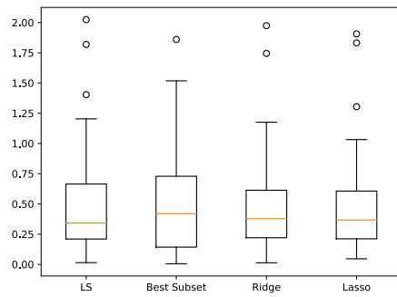
Figure 11.12: Boxplot displaying (absolute value of) prediction errors on the prostate cancer test set for di!erent regression methods. Generated by prostate\_comparison.ipynb.

11.4.6 Variable selection consistency

It is common to use ω¹ regularization to estimate the set of relevant variables, a process known as variable selection. A method that can recover the true set of relevant variables (i.e., the support of w↓) in the N ↔︎ ∈ limit is called model selection consistent. (This is a theoretical notion that assumes the data comes from the model.)

Let us give an example. We first generate a sparse signal w^↓ of size D = 4096, consisting of 160 randomly placed ±1 spikes. Next we generate a random design matrix X of size N ↓ D, where ^N = 1024. Finally we generate a noisy observation ^{y = X}w^{↓ +} ,, where ^{▷n ⇒ N} (0, ⁰.012). We then estimate w from y and X. The original w^↓ is shown in the first row of Figure 11.13. The second row is the ω¹ estimate wˆ ^L1 using φ = 0.1φmax. We see that this has “spikes” in the right places, so it has correctly identified the relevant variables. However, although we see that wˆ ^L1 has correctly identified the non-zero components, but they are too small, due to shrinkage. In the third row, we show the results of using the debiasing technique discussed in Section 11.4.3. This shows that we can recover the original weight vector. By contrast, the final row shows the OLS estimate, which is dense. Furthermore, it is visually clear that there is no single threshold value we can apply to wˆ mle to recover the correct sparse weight vector.

To use lasso to perform variable selection, we have to pick φ. It is common to use cross validation to pick the optimal value on the regularization path. However, it is important to note that cross validation is picking a value of φ that results in good predictive accuracy. This is not usually the same value as the one that is likely to recover the “true” model. To see why, recall that ω¹ regularization performs selection and shrinkage, that is, the chosen coe”cients are brought closer to 0. In order to prevent relevant coe”cients from being shrunk in this way, cross validation will tend to pick a value of φ that is not too large. Of course, this will result in a less sparse model which contains irrelevant variables (false positives). Indeed, it was proved in [MB06] that the prediction-optimal value of φ does not result in model selection consistency. However, various extensions to the basic method have been devised that are model selection consistent (see e.g., [BG11; HTW15]).

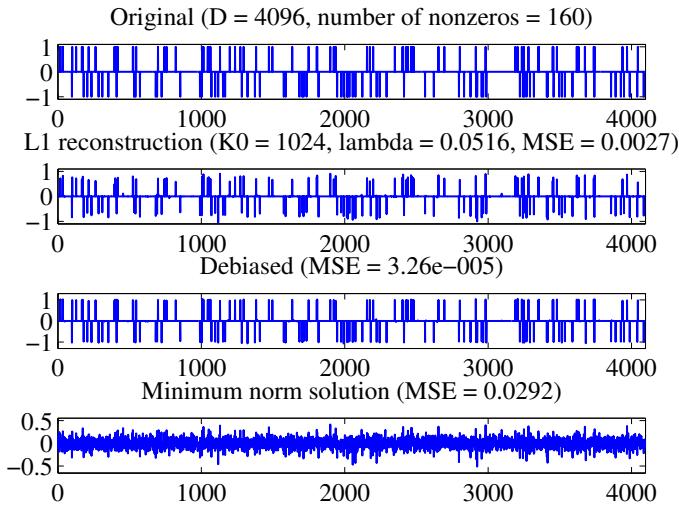
Figure 11.13: Example of recovering a sparse signal using lasso. See text for details. Adapted from Figure 1 of [FNW07]. Generated by sparse\_sensing\_demo.ipynb.

11.4.7 Group lasso

In standard ω¹ regularization, we assume that there is a 1:1 correspondence between parameters and variables, so that if wˆ^d = 0, we interpret this to mean that variable d is excluded. But in more complex models, there may be many parameters associated with a given variable. In particular, each variable d may have a vector of weights w^d associated with it, so the overall weight vector has block structure, w = [w1, w2,…, wD]. If we want to exclude variable d, we have to force the whole subvector w^d to go to zero. This is called group sparsity.

11.4.7.1 Applications

Here are some examples where group sparsity is useful:

• Linear regression with categorical inputs: If the d’th variable is categorical with K possible levels, then it will be represented as a one-hot vector of length K (Section 1.5.3.1), so to exclude variable d, we have to set the whole vector of incoming weights to 0.
• Multinomial logistic regression: The d’th variable will be associated with C di!erent weights, one per class (Section 10.3), so to exclude variable d, we have to set the whole vector of outgoing weights to 0.
• Neural networks: the k’th neuron will have multiple inputs, so if we want to “turn the neuron o!”, we have to set all the incoming weights to zero. This allows us to use group sparsity to learn neural network structure (for details, see e.g., [GEH19]).

• Multi-task learning: each input feature is associated with C di!erent weights, one per output task. If we want to use a feature for all of the tasks or none of the tasks, we should select weights at the group level [OTJ07].

11.4.7.2 Penalizing the two-norm

To encourage group sparsity, we partition the parameter vector into G groups, w = [w1,…, wG]. Then we minimize the following objective

\[\text{PNLL}(w) = \text{NLL}(w) + \lambda \sum\_{g=1}^{G} ||w\_g||\_2 \tag{11.97}\]

where ||wg||² = G$ ^d↑^{g w2 d} is the 2-norm of the group weight vector. If the NLL is least squares, this method is called group lasso [YL06; Kyu+10].

Note that if we had used the sum of the squared 2-norms in Equation (11.97), then the model would become equivalent to ridge regression, since

\[\sum\_{g=1}^{G} ||\mathbf{w}\_g||\_2^2 = \sum\_{g} \sum\_{d \in g} w\_d^2 = ||\mathbf{w}||\_2^2 \tag{11.98}\]

By using the square root, we are penalizing the radius of a ball containing the group’s weight vector: the only way for the radius to be small is if all elements are small.

Another way to see why the square root version enforces sparsity at the group level is to consider the gradient of the objective. Suppose there is only one group of two variables, so the penalty has the form -w^{2 1} + w^{2 2}. The derivative wrt w¹ is

\[\frac{\partial}{\partial w\_1} (w\_1^2 + w\_2^2)^{\frac{1}{2}} = \frac{w\_1}{\sqrt{w\_1^2 + w\_2^2}}\tag{11.99}\]

If w² is close to zero, then the derivative approaches 1, and w¹ is driven to zero as well, with force proportional to φ. If, however, w² is large, the derivative approaches 0, and w¹ is free to stay large as well. So all the coe”cients in the group will have similar size.

11.4.7.3 Penalizing the infinity norm

A variant of this technique replaces the 2-norm with the infinity-norm [TVW05; ZRY05]:

\[||\mathbf{w}\_g||\_\infty = \max\_{d \in g} |w\_d|\tag{11.100}\]

It is clear that this will also result in group sparsity, since if the largest element in the group is forced to zero, all the smaller ones will be as well.

11.4.7.4 Example

An illustration of these techniques is shown in Figure 11.14 and Figure 11.15. We have a true signal w of size D = 2¹² = 4096, divided into 64 groups each of size 64. We randomly choose 8 groups

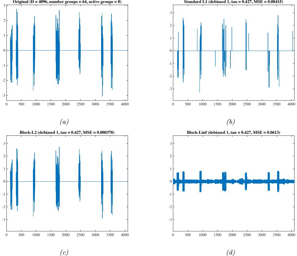
Figure 11.14: Illustration of group lasso where the original signal is piecewise Gaussian. (a) Original signal. (b) Vanilla lasso estimate. (c) Group lasso estimate using an ,² norm on the blocks. (d) Group lasso estimate using an ,^↑ norm on the blocks. Adapted from Figures 3-4 of [WNF09]. Generated by groupLassoDemo.ipynb.

of w and assign them non-zero values. In Figure 11.14 the values are drawn from a N (0, 1); in Figure 11.15, the values are all set to 1. We then sample a random design matrix X of size N ↓ D, where ^N = 2¹⁰ = 1024. Finally, we generate ^{y = Xw +} ,, where , ^{⇒ N} (0, ¹⁰→4I^N ). Given this data, we estimate the support of w using ω¹ or group ω1, and then estimate the non-zero values using least squares (debiased estimate).

We see from the figures that group lasso does a much better job than vanilla lasso, since it respects the known group structure. We also see that the ω↘ norm has a tendency to make all the elements within a block to have similar magnitude. This is appropriate in the second example, but not the first. (The value of φ was the same in all examples, and was chosen by hand.)

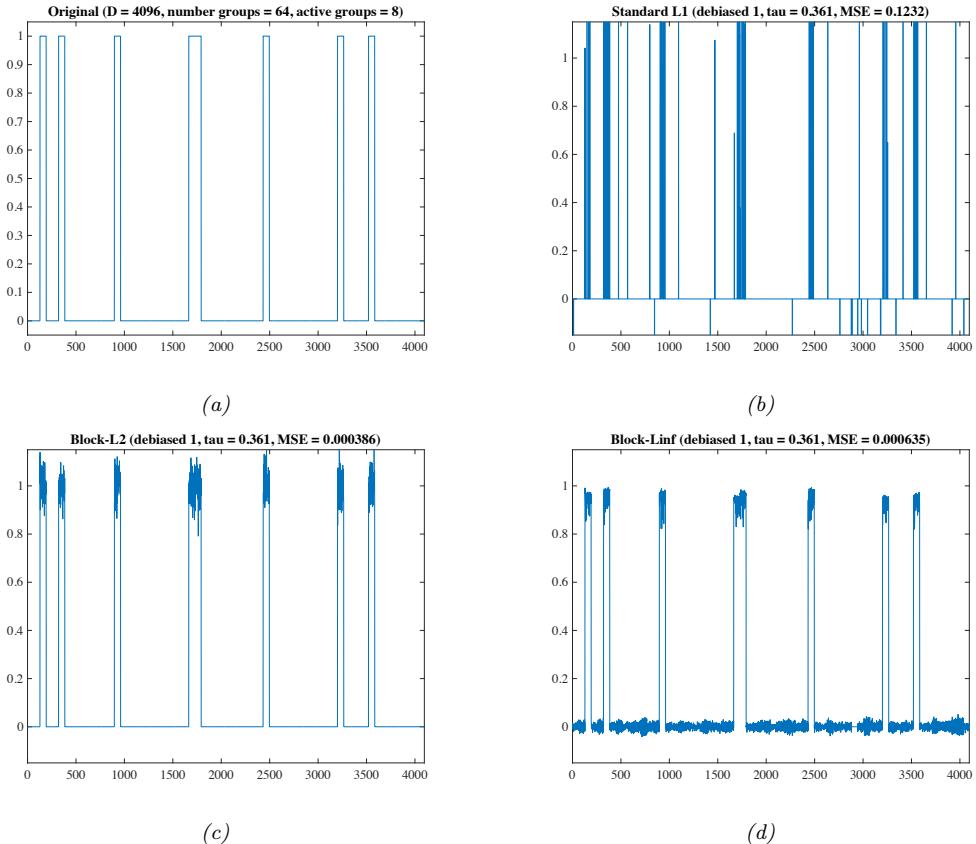
Figure 11.15: Same as Figure 11.14, except the original signal is piecewise constant. Generated by groupLassoDemo.ipynb.

11.4.8 Elastic net (ridge and lasso combined)

In group lasso, we need to specify the group structure ahead of time. For some problems, we don’t know the group structure, and yet we would still like highly correlated coe”cients to be treated as an implicit group. One way to achieve this e!ect, proposed in [ZH05], is to use the elastic net, which is a hybrid between lasso and ridge regression.3 This corresponds to minimizing the following objective:

\[\mathcal{L}(\mathbf{w}, \lambda\_1, \lambda\_2) = ||\mathbf{y} - \mathbf{X}\mathbf{w}||^2 + \lambda\_2 ||\mathbf{w}||\_2^2 + \lambda\_1 ||\mathbf{w}||\_1 \tag{11.101}\]

This penalty function is strictly convex (assuming φ² > 0) so there is a unique global minimum, even if X is not full rank. It can be shown [ZH05] that any strictly convex penalty on w will exhibit a grouping e”ect, which means that the regression coe”cients of highly correlated variables tend to

^3. It is apparently called the “elastic net” because it is “like a stretchable fishing net that retains all the big fish” [ZH05].

be equal. In particular, if two features are identically equal, so X:^j = X:k, one can show that their estimates are also equal, wˆ^j = wˆk. By contrast, with lasso, we may have that wˆ^j = 0 and wˆ^k ↗= 0 or vice versa, resulting in less stable estimates.

In addition to its soft grouping behavior, elastic net has other advantages. In particular, if D>N, the maximum number of non-zero elements that can be selected (excluding the MLE, which has D non-zero elements) is N. By contrast, elastic net can select more than N non-zero variables on its path to the dense estimate, thus exploring more possible subsets of variables.

11.4.9 Optimization algorithms

A large variety of algorithms have been proposed to solve the lasso problem, and other ω1-regularized convex objectives. In this section, we briefly mention some of the most popular methods.

11.4.9.1 Coordinate descent

Sometimes it is hard to optimize all the variables simultaneously, but it easy to optimize them one by one. In particular, we can solve for the j’th coe”cient with all the others held fixed as follows:

\[w\_j^\* = \operatorname\*{argmin}\_{\eta} \mathcal{L}(w + \eta e\_j) \tag{11.102}\]

where e^j is the j’th unit vector. This is called coordinate descent. We can either cycle through the coordinates in a deterministic fashion, or we can sample them at random, or we can choose to update the coordinate for which the gradient is steepest.

This method is particularly appealing if each one-dimensional optimization problem can be solved analytically, as is the case for lasso (see Equation (11.87)). This is known as the shooting algorithm [Fu98; WL08]. (The term “shooting” is a reference to cowboy theme inspired by the term “lasso”.) See Algorithm 11.1 for details.

This coordinate descent method has been generalized to the GLM case in [FHT10], and is the basis of the popular glmnet software library.

Algorithm 11.1: Coordinate descent for lasso (aka shooting algorithm)

¹ Initialize w = (X^TX + φI)→¹X^Ty ² repeat ³ for d = 1,…,D do ⁴ a^d = $^{N n}=1 x² nd ⁵ c^d = $^{N n}=1 ^xnd(y^{n ↑ wT}x^{n + w}dxnd) ⁶ w^d = SoftThreshold( ^{cd ad} , φ/ad) ⁷ until converged

11.4.9.2 Projected gradient descent

In this section, we convert the non-di!erentiable ω¹ penalty into a smooth regularizer. To do this, we first use the split variable trick to define ^w = ^{w+ ↑ w}→, where ^w+ = max{w, 0} and

^{w→ = ↑} min{w, ⁰}. Now we can replace ||w||¹ with $ d(w^{+ d} + w^{→ d} ). We also have to replace NLL(w) with NLL(w⁺ + w→). Thus we get the following smooth, but constrained, optimization problem:

\[\min\_{\mathbf{w}^+ \ge 0, \mathbf{w}^- \ge 0} \text{NLL}(\mathbf{w}^+ - \mathbf{w}^-) + \lambda \sum\_{d=1}^D (w\_d^+ + w\_d^-) \tag{11.103}\]

In this case of a Gaussian likelihood, the NLL becomes a least squares loss, and the objective becomes a quadratic program (Section 8.5.4). One way to solve such problems is to use projected gradient descent (Section 8.6.1). Specifically, we can enforce the constraint by projecting onto the positive orthant, which we can do using w^d := max(wd, 0); this operation is denoted by P+. Thus the projected gradient update takes the following form:

\[\begin{pmatrix} \mathbf{w}\_{t+1}^{+}\\\mathbf{w}\_{t+1}^{-} \end{pmatrix} = P\_{+} \begin{pmatrix} \left[ \mathbf{w}\_{t}^{+} - \eta\_{t} \nabla \text{NLL} (\mathbf{w}\_{t}^{+} - \mathbf{w}\_{t}^{-}) - \eta\_{t} \lambda \mathbf{e} \right] \\\left[ \mathbf{w}\_{t}^{-} + \eta\_{t} \nabla \text{NLL} (\mathbf{w}\_{t}^{+} - \mathbf{w}\_{t}^{-}) - \eta\_{t} \lambda \mathbf{e} \right] \end{pmatrix} \tag{11.104}\]

where e is the unit vector of all ones.

11.4.9.3 Proximal gradient descent

In Section 8.6, we introduced proximal gradient descent, which can be used to optimize smooth functions with non-smooth penalties, such as ω1. In Section 8.6.2, we showed that the proximal operator for the ω¹ penalty corresponds to soft thresholding. Thus the proximal gradient descent update can be written as

\[w\_{t+1} = \text{SoftThreshold}(w\_t - \eta\_t \nabla \text{NLL}(w\_t), \eta\_t \lambda) \tag{11.105}\]

where the soft thresholding operator (Equation (8.134)) is applied elementwise. This is called the iterative soft thresholding algorithm or ISTA [DDDM04; Don95]. If we combine this with Nesterov acceleration, we get the method known as “fast ISTA” or FISTA [BT09], which is widely used to fit sparse linear models.

11.4.9.4 LARS

In this section, we discuss methods that can generate a set of solutions for di!erent values of φ, starting with the empty set, i.e., they compute the full regularization path (Section 11.4.4). These algorithms exploit the fact that one can quickly compute wˆ (φk) from wˆ (φ^k→1) if φ^k ↖ φ^k→1; this is known as warm starting. In fact, even if we only want the solution for a single value of φ, call it φ↓, it can sometimes be computationally more e”cient to compute a set of solutions, from φmax down to φ↓, using warm-starting; this is called a continuation method or homotopy method. This is often much faster than directly “cold-starting” at φ↓; this is particularly true if φ^↓ is small.

The LARS algorithm [Efr+04], which stands for “least angle regression and shrinkage”, is an example of a homotopy method for the lasso problem. This can compute wˆ (φ) for all possible values of φ in an e”cient manner. (A similar algorithm was independently invented in [OPT00b; OPT00a]).

LARS works as follows. It starts with a large value of φ, such that only the variable that is most correlated with the response vector y is chosen. Then φ is decreased until a second variable is found which has the same correlation (in terms of magnitude) with the current residual as the first variable, where the residual at step k on the path is defined as r^k = y ↑ X:,Fkwk, where F^k is the current active set (cf., Equation (11.83)). Remarkably, one can solve for this new value of φ analytically, by using a geometric argument (hence the term “least angle”). This allows the algorithm to quickly “jump” to the next point on the regularization path where the active set changes. This repeats until all the variables are added.

It is necessary to allow variables to be removed from the current active set, even as we increase φ, if we want the sequence of solutions to correspond to the regularization path of lasso. If we disallow variable removal, we get a slightly di!erent algorithm called least angle regression or LAR. LAR is very similar to greedy forward selection, and a method known as least squares boosting (see e.g., [HTW15]).

11.5 Regression splines *

We have seen how we can use polynomial basis functions to create nonlinear mappings from input to output, even though the model remains linear in the parameters. One problem with polynomials is that they are a global approximation to the function. We can achieve more flexibility by using a series of local approximations. To do this, we just need to define a set of basis functions that have local support. The notion of “locality” is hard to define in high-dimensional input spaces, so in this section, we restrict ourselves to 1d inputs. We can then approximate the function using

\[f(x; \theta) = \sum\_{i=1}^{m} w\_i B\_i(x) \tag{11.106}\]

where Bⁱ is the i’th basis function.

A common way to define such basis functions is to use B-splines. (“B” stands for “basis”, and the term “spline” refers to a flexible piece of material used by artists to draw curves.) We discuss this in more detail in Section 11.5.1.

11.5.1 B-spline basis functions

A spline is a piecewise polynomial of degree D, where the locations of the pieces are defined by a set of knots, t¹ < ··· < tm. More precisely, the polynomial is defined on each of the intervals (↑∈, t1), [t1, t2], ··· , [tm, ∈). The function is continuous and has continuous derivatives of orders 1,…,D ↑ 1 at its knot points. It is common to use cubic splines, in which D = 3. This ensures the function is continuous, and has continuous first and second derivatives at each knot.

We will skip the details on how B-splines are computed, since it is not relevant to our purposes. Su”ce it to say that we can call the patsy.bs function to convert the N ↓ 1 data matrix X into an N ↓(K +D+ 1) design matrix B, where K is the number of knots and D is the degree. (Alternatively, you can specify the desired number of basis functions, and let patsy work out the number and locations of the knots.)

Figure 11.16 illustrates this approach, where we use B-splines of degree 0, 1 and 3, with 3 knots. By taking a weighted combination of these basis functions, we can get increasingly smooth functions, as shown in the bottom row.

We see from Figure 11.16 that each individual basis function has local support. At any given input point x, only D + 1 basis functions will be “active”. This is more obvious if we plot the design matrix

Figure 11.16: Illustration of B-splines of degree 0, 1 and 3. Top row: unweighted basis functions. Dots mark the locations of the 3 internal knots at [0.25, 0.5, 0.75]. Bottom row: weighted combination of basis functions using random weights. Generated by splines\_basis\_weighted.ipynb. Adapted from Figure 5.4 of [MKL11]. Used with kind permission of Osvaldo Martin.

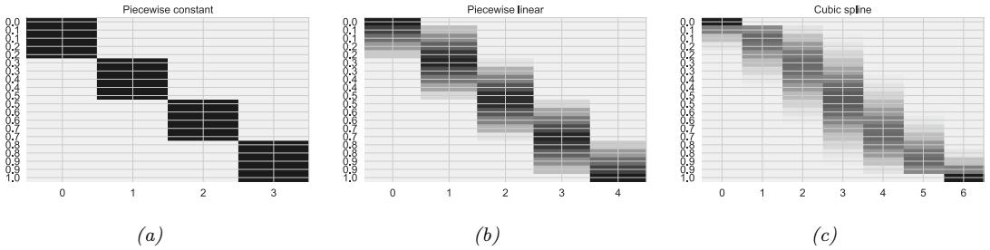
Figure 11.17: Design matrix for B-splines of degree (a) 0, (b) 1 and (c) 3. We evaluate the splines on 20 inputs ranging from 0 to 1. Generated by splines\_basis\_heatmap.ipynb. Adapted from Figure 5.6 of [MKL11]. Used with kind permission of Osvaldo Martin.

B itself. Let us first consider the piecewise constant spline, shown in Figure 11.17(a). The first B-spline (column 1) is 1 for the first 5 observations, and otherwise 0. The second B-spline (column 0) is 0 for the first 5 observations, 1 for the second 5, and then 0 again. And so on. Now consider the linear spline, shown in Figure 11.17(b). The first B-spline (column 0) goes from 1 to 0, the next three splines go from 0 to 1 and back to 0; and the last spline (column 4) goes from 0 to 1; this reflects the triangular shapes shown in the top middle panel of Figure 11.16. Finally consider the cubic spline, shown in Figure 11.17(c). Here the pattern of activations is smoother, and the resulting model fits will be smoother too.

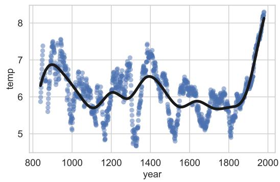
Figure 11.18: Fitting a cubic spline regression model with 15 knots to a 1d dataset. Generated by splines\_cherry\_blossoms.ipynb. Adapted from Figure 5.3 of [McE20].

11.5.2 Fitting a linear model using a spline basis

Once we have computed the design matrix B, we can use it to fit a linear model using least squares or ridge regression. (It is usually best to use some regularization.) As an example, we consider a dataset from [McE20, Sec 4.5], which records the the first day of the year, and the corresponding temperature, that marks the start of the cherry blossom season in Japan. (We use this dataset since it has interesting semi-periodic structure.) We fit the data using a cubic spline. We pick 15 knots, spaced according to quantiles of the data. The results are shown in Figure 11.18. We see that the fit is reasonable. Using more knots would improve the quality of the fit, but would eventually result in overfitting. We can select the number of knots using a model selection method, such as grid search plus cross validation.

11.5.3 Smoothing splines

Smoothing splines are related to regression splines, but use N knots, where N is the number of datapoints. That is, they are non-parametric models, since the number of parameters grows with the size of the data, rather than being fixed a priori. To avoid overfitting, smoothing splines rely on ω² regularization. This technique is closely related to Gaussian process regression, which we discuss in Section 17.2.

11.5.4 Generalized additive models

A generalized additive model or GAM extends spline regression to the case of multidimensional inputs [HT90]. It does this by ignoring interactions between the inputs, and assuming the function has the following additive form:

\[f(x; \theta) = \alpha + \sum\_{d=1}^{D} f\_d(x\_d) \tag{11.107}\]

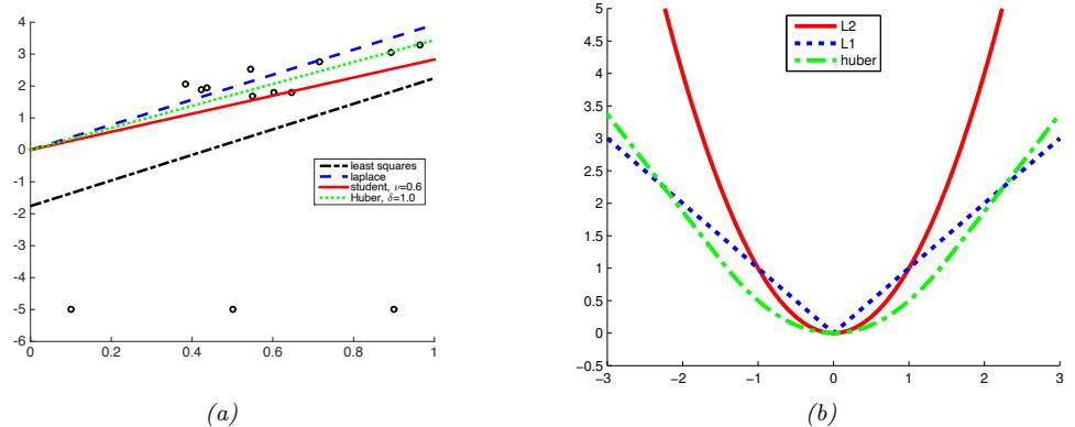
Figure 11.19: (a) Illustration of robust linear regression. Generated by linregRobustDemoCombined.ipynb. (b) Illustration of ,2, ,1, and Huber loss functions with ◁ = 1.5. Generated by huberLossPlot.ipynb.

where each f^d is a regression or smoothing spline. This model can be fit using backfitting, which iteratively fits each f^d to the partial residuals generated by the other terms. We can extend GAMs beyond the regression case (e.g., to classification) by using a link function, as in generalized linear models (Chapter 12).

11.6 Robust linear regression *

It is very common to model the noise in regression models using a Gaussian distribution with zero mean and constant variance, ^{rn ⇒ N} (0, ^ε2), where ^rn = ^{yn ↑ wT}xn. In this case, maximizing likelihood is equivalent to minimizing the sum of squared residuals, as we have seen. However, if we have outliers in our data, this can result in a poor fit, as illustrated in Figure 11.19(a). (The outliers are the points on the bottom of the figure.) This is because squared error penalizes deviations quadratically, so points far from the line have more e!ect on the fit than points near to the line.

One way to achieve robustness to outliers is to replace the Gaussian distribution for the response variable with a distribution that has heavy tails. Such a distribution will assign higher likelihood to outliers, without having to perturb the straight line to “explain” them. We discuss several possible alternative probability distributions for the response variable below; see Table 11.2 for a summary.

11.6.1 Laplace likelihood

In Section 2.7.3, we noted that the Laplace distribution is also robust to outliers. If we use this as our observation model for regression, we get the following likelihood:

\[p(y|\mathbf{z}, \mathbf{w}, b) = \text{Laplace}(y|\mathbf{w}^\top \mathbf{z}, b) \propto \exp(-\frac{1}{b}|y - \mathbf{w}^\top \mathbf{z}|) \tag{11.108}\]

The robustness arises from the use of ^{|y ↑ wT}x^| instead of (^{y ↑ wT}x)². Figure 11.19(a) gives an example of the method in action.

Likelihood	Prior	Posterior	Name	Section
Gaussian	Uniform	Point	Least squares	11.2.2
Student	Uniform	Point	Robust regression	11.6.2
Laplace	Uniform	Point	Robust regression	11.6.1
Gaussian	Gaussian	Point	Ridge	11.3
Gaussian	Laplace	Point	Lasso	11.4
Gaussian	Gauss-Gamma	Gauss-Gamma	Bayesian lin. reg	11.7

Table 11.2: Summary of various likelihoods, priors and posteriors used for linear regression. The likelihood refers to the distributional form of ^p(y|x, ^w, ^ϑ2), and the prior refers to the distributional form of ^p(w). The posterior refers to the distributional form of p(w|D). “Point” stands for the degenerate distribution ◁(w ↑ wˆ ), where wˆ is the MAP estimate. MLE is equivalent to using a point posterior and a uniform prior.

11.6.1.1 Computing the MLE using linear programming

We can compute the MLE for this model using linear programming. As we explain in Section 8.5.3, this is a way to solve a constrained optimization problems of the form

\[\underset{\mathbf{v}}{\operatorname\*{argmin}} \mathbf{c}^{\mathsf{T}} \mathbf{v} \quad \text{s.t.} \quad \mathbf{A} \mathbf{v} \le \mathbf{b} \tag{11.109}\]

where ^{v → Rn} is the set of ⁿ unknown parameters, ^cTv is the linear objective function we want to minimize, and a^{T i} v ↘ bⁱ is a set of m linear constraints we must satisfy. To apply this to our problem, let us define ^v = (w1,…,wD, e1,…,e^N ) ^{→ RD}+^N , where ^ei = ^|y^{i ↑ y}ˆi^| is the residual error for example ⁱ. We want to minimize the sum of the residuals, so we define ^c = (0, ··· , ⁰, ¹, ··· , 1) ^{→ RD}+^N , where the first D elements are 0, and the last N elements are 1.

We need to enforce the constraint that eⁱ = |yˆⁱ ↑yi|. In fact it is su”cient to enforce the constraint that ^|w^Tx^{i ↑ y}i^| ↘ ^ei, since minimizing the sum of the ^ei’s will “push down” on this constraint and make it tight. Since ^|a^| ↘ ^b =∝ ↑^b ↘ ^a ↘ ^b, we can encode ^|w^Tx^{i ↑ y}i^| ↘ ^ei as two linear constraints:

\[\mathbf{w}\_{i} \ge \mathbf{w}^{\mathsf{T}} \mathbf{x}\_{i} - y\_{i} \tag{11.110}\]

\[e\_i \ge -(w^\top x\_i - y\_i) \tag{11.111}\]

We can write Equation (11.110) as

\[\left(x\_i, 0, \cdots, 0, -1, 0, \cdots, 0\right)^{\mathsf{T}} \boldsymbol{\mathfrak{v}} \le y\_i \tag{11.112}\]

where the first D entries are filled with xi, and the ↑1 is in the (D + i)’th entry of the vector. Similarly we can write Equation (11.111) as

\[\begin{pmatrix} -x\_i, 0, \cdots, 0, -1, 0, \cdots, 0 \end{pmatrix}^{\mathsf{T}} v \le -y\_i \tag{11.113}\]

We can write these constraints in the form ^Av ↘ ^b by defining ^{A → R}2N↔︎(N+D) as follows:

\[\mathbf{A} = \begin{pmatrix} x\_1 & -1 & 0 & 0 & \cdots & 0 \\ -x\_1 & -1 & 0 & 0 & \cdots & 0 \\ x\_2 & 0 & -1 & 0 & \cdots & 0 \\ -x\_2 & 0 & -1 & 0 & \cdots & 0 \\ & & & \vdots & & & \end{pmatrix} \tag{11.114}\]

and defining ^{b → R2N} as

\[\mathbf{b} = \begin{pmatrix} y\_1, -y\_1, y\_2, -y\_2, \dots, -y\_N, -y\_N \end{pmatrix} \tag{11.115}\]

11.6.2 Student-t likelihood

In Section 2.7.1, we discussed the robustness properties of the Student distribution. To use this in a regression context, we can just make the mean be a linear function of the inputs, as proposed in [Zel76]:

\[p(y|\mathbf{x}, \mathbf{w}, \sigma^2, \nu) = \mathcal{T}(y|\mathbf{w}^\mathsf{T}\mathbf{x}, \sigma^2, \nu) \tag{11.116}\]

We can fit this model using SGD or EM (see [Mur23] for details).

11.6.3 Huber loss

An alternative to minimizing the NLL using a Laplace or Student likelihood is to use the Huber loss, which is defined as follows:

\[\ell\_{\text{huber}}(r,\delta) = \begin{cases} |r^2/2 & \text{if } |r| \le \delta \\ \delta|r| - \delta^2/2 & \text{if } |r| > \delta \end{cases} \tag{11.117}\]

This is equivalent to ω² for errors that are smaller than ↽, and is equivalent to ω¹ for larger errors. See Figure 5.3 for a plot.

The advantage of this loss function is that it is everywhere di!erentiable. Consequently optimizing the Huber loss is much faster than using the Laplace likelihood, since we can use standard smooth optimization methods (such as SGD) instead of linear programming. Figure 11.19 gives an illustration of the Huber loss function in action. The results are qualitatively similiar to the Laplace and Student methods.

The parameter ↽, which controls the degree of robustness, is usually set by hand, or by crossvalidation. However, [Bar19] shows how to approximate the Huber loss such that we can optimize ↽ by gradient methods.

11.6.4 RANSAC

In the computer vision community, a common approach to robust regression is to use RANSAC, which stands for “random sample consensus” [FB81]. This works as follows: we sample a small initial set of points, fit the model to them, identify outliers wrt this model (based on large residuals), remove

the outliers, and then refit the model to the inliers. We repeat this for many random initial sets and pick the best model.

A deterministic alternative to RANSAC is the following iterative scheme: intially we assume that all datapoints are inliers, and we fit the model to compute wˆ ⁰; then, for each iteration t, we identify the outlier points as those with large residual under the model wˆ ^t, remove them, and refit the model to the remaining points to get wˆ ^t+1. Even though this hard thresholding scheme makes the problem nonconvex, this simple scheme can be proved to rapidly converge to the optimal estimate under some reasonable assumptions [Muk+19; Sug+19].

11.7 Bayesian linear regression *

We have seen how to compute the MLE and MAP estimate for linear regression models under various priors. In this section, we discuss how to compute the posterior over the parameters, p(ω|D). For simplicity, we assume the variance is known, so we just want to compute ^p(w|D, ^ε2). See the sequel to this book, [Mur23], for the general case.

11.7.1 Priors

For simplicity, we will use a Gaussian prior:

\[p(w) = \mathcal{N}(w \mid \check{w}, \check{\Sigma}) \tag{11.118}\]

This is a small generalization of the prior that we use in ridge regression (Section 11.3). See the sequel to this book, [Mur23], for a discussion of other priors.

11.7.2 Posteriors

We can rewrite the likelihood in terms of an MVN as follows:

\[p(\mathcal{D}|\mathbf{w}, \sigma^2) = \prod\_{n=1}^{N} p(y\_n|\mathbf{w}^\mathsf{T}\mathbf{z}, \sigma^2) = \mathcal{N}(y|\mathbf{X}\mathbf{w}, \sigma^2\mathbf{I}\_N) \tag{11.119}\]

where I^N is the N ↓ N identity matrix. We can then use Bayes rule for Gaussians (Equation (3.37)) to derive the posterior, which is as follows:

\[p(w|\mathbf{X}, \mathbf{y}, \sigma^2) \propto \mathcal{N}(w|\; \Psi, \dot{\Sigma}) \mathcal{N}(y|\mathbf{X}w, \sigma^2 \mathbf{I}\_N) = \mathcal{N}(w|\; \Psi, \dot{\Sigma}) \tag{11.120}\]

\[ \hat{\boldsymbol{w}} \triangleq \hat{\boldsymbol{\Sigma}} \left( \check{\boldsymbol{\Sigma}}^{-1} \check{\boldsymbol{w}} + \frac{1}{\sigma^2} \mathbf{X}^{\mathsf{T}} \boldsymbol{y} \right) \tag{11.121} \]

\[ \hat{\boldsymbol{\Sigma}} \stackrel{\scriptstyle \Delta}{=} (\check{\boldsymbol{\Sigma}}^{-1} + \frac{1}{\sigma^2} \mathbf{X}^{\mathsf{T}} \mathbf{X})^{-1} \tag{11.122} \]

where ↭w is the posterior mean, and ↭ ! is the posterior covariance.

If ↫w= 0 and ↫ != τ ²I, then the posterior mean becomes ↭w= ¹ ε² ↭ ! X^Ty. If we define φ = ^{ε2 ς2} , we recover the ridge regression estimate, ↭w= (φI + X^TX)→¹X^Ty, which matches Equation (11.57).

11.7.3 Example

Suppose we have a 1d regression model of the form f(x; w) = w⁰ + w1x1, where the true parameters are w⁰ = ↑0.3 and w¹ = 0.5. We now perform inference p(w|D) and visualize the 2d prior and posterior as the size of the training set N increases.

In particular, in Figure 11.20 (which inspired the front cover of this book), we plot the likelihood, the posterior, and an approximation to the posterior predictive distribution.4 Each row plots these distributions as we increase the amount of training data, N. We now explain each row:

• In the first row, N = 0, so the posterior is the same as the prior. In this case, our predictions are “all over the place”, since our prior is essentially uniform.
• In the second row, N = 1, so we have seen one data point (the blue circle in the plot in the third column). Our posterior becomes constrained by the corresponding likelihood, and our predictions pass close to the observed data. However, we see that the posterior has a ridge-like shape, reflecting the fact that there are many possible solutions, with di!erent slopes/intercepts. This makes sense since we cannot uniquely infer two parameters (w⁰ and w1) from one observation.
• In the third row, N = 2. In this case, the posterior becomes much narrower since we have two constraints from the likelihood. Our predictions about the future are all now closer to the training data.
• In the fourth (last) row, N = 100. Now the posterior is essentially a delta function, centered on the true value of w^↓ = (↑0.3, 0.5), indicated by a white cross in the plots in the first and second columns. The variation in our predictions is due to the inherent Gaussian noise with magnitude ε².

This example illustrates that, as the amount of data increases, the posterior mean estimate, ↭µ^{= E} [w|D], converges to the true value ^w↓ that generated the data. We thus say that the Bayesian estimate is a consistent estimator (see Section 5.3.2 for more details). We also see that our posterior uncertainty decreases over time. This is what we mean when we say we are “learning” about the parameters as we see more data.

11.7.4 Computing the posterior predictive

We have discussed how to compute our uncertainty about the parameters of the model, p(w|D). But what about the uncertainty associated with our predictions about future outputs? Using Equation (3.38), we can show that the posterior predictive distribution at a test point x is also Gaussian:

\[p(y|\mathbf{z}, \mathcal{D}, \sigma^2) = \int \mathcal{N}(y|\mathbf{z}^\mathsf{T}w, \sigma^2) \mathcal{N}(w|\,\widehat{\mu}, \widehat{\Sigma}) dw \tag{11.123}\]

\[=N(y|\:\hat{\mu}^{\mathsf{T}}\:\!x,\hat{\sigma}^{2}\:\!(\mathsf{x}))\tag{11.124}\]

^4. To approximate this, we draw some samples from the posterior, w^s ↗ N (µ, !), and then plot the line E [y|x, ws], where x ranges over [↔︎1, 1], for each sampled parameter value.

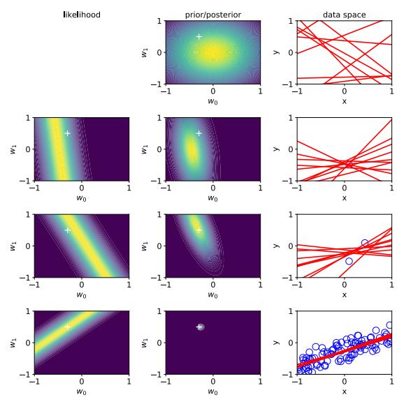
Figure 11.20: Sequential Bayesian inference of the parameters of a linear regression model p(y|x) = N (y|w⁰ + w1x1, ϑ²). Left column: likelihood function for current data point. Middle column: posterior given first N data points, ^p(w0, w1|x1:^N , y1:^N , ^ϑ2). Right column: samples from the current posterior predictive distribution. Row 1: prior distribution (N = 0). Row 2: after 1 data point. Row 3: after 2 data points. Row 4: after 100 data points. The white cross in columns 1 and 2 represents the true parameter value; we see that the mode of the posterior rapidly converges to this point. The blue circles in column 3 are the observed data points. Adapted from Figure 3.7 of [Bis06]. Generated by linreg\_2d\_bayes\_demo.ipynb.

where ↭ε² (x) ↭ ^ε2 + ^xT ↭ ! x is the variance of the posterior predictive distribution at point x after seeing the N training examples. The predicted variance depends on two terms: the variance of the observation noise, ε², and the variance in the parameters, ↭ !. The latter translates into variance about observations in a way which depends on how close x is to the training data D. This is illustrated in Figure 11.21(b), where we see that the error bars get larger as we move away from the training points, representing increased uncertainty. This can be important for certain applications, such as active learning, where we choose where to collect training data (see Section 19.4).

In some cases, it is computationally intractable to compute the parameter posterior, p(w|D). In such cases, we may choose to use a point estimate, wˆ , and then to use the plugin approximation. This gives

\[p(y|\mathbf{z}, \mathcal{D}, \sigma^2) = \int \mathcal{N}(y|\mathbf{z}^\mathsf{T}w, \sigma^2) \delta(w - \hat{w}) dw = p(y|\mathbf{z}^\mathsf{T}\hat{w}, \sigma^2). \tag{11.125}\]

We see that the posterior predictive variance is constant, and independent of the data, as illustrated in Figure 11.21(a). If we sample a parameter from this posterior, we will always recover a single function, as shown in Figure 11.21(c). By contrast, if we sample from the true posterior, ^{ws ⇒ p}(w|D, ^ε2), we will get a range of di!erent functions, as shown in Figure 11.21(d), which more accurately reflects our uncertainty.

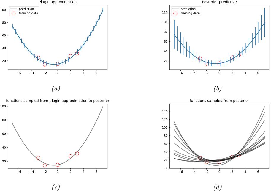
Figure 11.21: (a) Plugin approximation to predictive density (we plug in the MLE of the parameters) when fitting a second degree polynomial to some 1d data. (b) Posterior predictive density, obtained by integrating out the parameters. Black curve is posterior mean, error bars are 2 standard deviations of the posterior predictive density. (c) 10 samples from the plugin approximation to posterior predictive distribution. (d) 10 samples from the true posterior predictive distribution. Generated by linreg\_post\_pred\_plot.ipynb.

11.7.5 The advantage of centering

The astute reader might notice that the shape of the 2d posterior in Figure 11.20 is an elongated ellipse (which eventually collapses to a point as N ↔︎ ∈). This implies that there is a lot of posterior correlation between the two parameters, which can cause computational di”culties.

To understand why this happens, note that each data point induces a likelihood function corresponding to a line which goes through that data point. When we look at all the data together, we see that predictions with maximum likelihood must correspond to lines that go through the mean of the data, (x, y). There are many such lines, but if we increase the slope, we must decrease the intercept. Thus we can think of the set of high probability lines as spinning around the data mean, like a wheel of fortune.5 This correlation between w⁰ and w¹ is why the posterior has the form of a diagonal line. (The Gaussian prior converts this into an elongated ellipse, but the posterior correlation still persists until the sample size causes the posterior to shrink to a point.)

It can be hard to compute such elongated posteriors. One simple solution is to center the input data, i.e., by using x↗ ⁿ = xⁿ ↑ x. Now the lines can pivot around the origin, reducing the posterior

^5. This analogy is from [Mar18, p96].

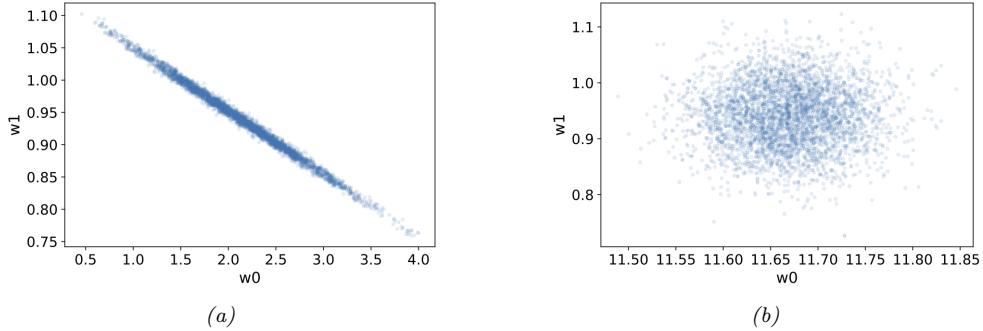
Figure 11.22: Posterior samples of p(w0, w1|D) for 1d linear regression model p(y|x, ω) = N (y|w⁰ + w1x, ϑ²) with a Gaussian prior. (a) Original data. (b) Centered data. Generated by linreg\_2d\_bayes\_centering\_pymc3.ipynb.

correlation between w⁰ and w1. See Figure 11.22 for an illustration. (We may also choose to divide each xⁿ by the standard deviation of that feature, as discussed in Section 10.2.8.)

Note that we can convert the posterior derived from fitting to the centered data back to the original coordinates by noting that

\[y' = w\_0' + w\_1'x' = w\_0' + w\_1'(x - \overline{x}) = (w\_0' - w\_1'\overline{x}) + w\_1'x \tag{11.126}\]

Thus the parameters on the uncentered data are w⁰ = w↗ ⁰ ↑ w↗ ¹x and w¹ = w↗ 1.

11.7.6 Dealing with multicollinearity

In many datasets, the input variables can be highly correlated with each other. Including all of them does not generally harm predictive accuracy (provided you use a suitable prior or regularizer to prevent overfitting). However, it can make interpretation of the coe”cients more di”cult.

To illustrate this, we use a toy example from [McE20, Sec 6.1]. Suppose we have a dataset of N people in which we record their heights hi, as well as the length of their left legs lⁱ and right legs ri. Suppose hⁱ ⇒ N (10, 2), so the average height is h = 10 (in unspecified units). Suppose the length of the legs is some fraction ςⁱ ⇒ Unif(0.4, 0.5) of the height, plus a bit of Gaussian noise, specifically lⁱ ⇒ N (ςihi, 0.02) and rⁱ ⇒ N (ςihi, 0.02).

Now suppose we want to predict the height of a person given measurement of their leg lengths. (I did mention this is a toy example!) Since both left and right legs are noisy measurements of the unknown quantity, it is useful to use both of them. So we use linear regression to fit ^p(h|l, r) = ^N (h|^{ϱ + 1}l^{l + 1}rr, ^ε2). We use vague priors, ^ϱ, ¹l, ^{1r ⇒ N} (0, 100), and ^{ε ⇒} Expon(1).

Since the average leg length is l = 0.45h = 4.5, we might expect each 1 coe”cient to be around h/l = 10/4.5=2.2. However, the posterior marginals shown in Figure 11.23 tell a di!erent story: we see that the posterior mean of 1^l is near 2.6, but 1^r is near -0.6. Thus it seems like the right leg feature is not needed. This is because the regression coe”cient for feature j encodes the value of knowing x^j given that all the other features x→^j are already known, as we discussed in Section 11.2.2.1. If we already know the left leg, the marginal value of also knowing the right leg is small. However, if we

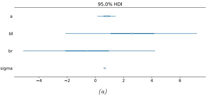
Figure 11.23: Posterior marginals for the parameters in the multi-leg example. Generated by multi\_collinear\_legs\_numpyro.ipynb.

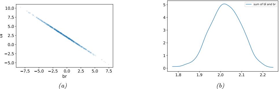
Figure 11.24: Posteriors for the multi-leg example. (a) Joint posterior p(⇀l, ⇀r|D) (b) Posterior of p(⇀^l + ⇀r|data). Generated by multi\_collinear\_legs\_numpyro.ipynb.

rerun this example with slightly di!erent data, we may reach the opposite conclusion, and favor the right leg over the left.

We can gain more insight by looking at the joint distribution p(1l, 1r|D), shown in Figure 11.24a. We see that the parameters are very highly correlated, so if 1^r is large, then 1^l is small, and vice versa. The marginal distribution for each parameter does not capture this. However, it does show that there is a lot of uncertainty about each parameter, showing that they are non-identifiable. However, their sum is well-determined, as can be seen from Figure 11.24b, where we plot p(1^l +1r|D); this is centered on 2.2, as we might expect.

This example goes to show that we must be careful trying to interpret the significance of individual coe”cient estimates in a model, since they do not mean much in isolation.

11.7.7 Automatic relevancy determination (ARD) *

Consider a linear regression model with known observation noise but unknown regression weights, ^N (y|Xw, ^ε2I). Suppose we use a Gaussian prior for the weights, ^{wj ⇒ N} (0, ¹/ϱ^j ), where ^ϱj is the

precision of the j’th parameter. Now suppose we estimate the prior precisions as follows:

\[\hat{\boldsymbol{\alpha}} = \operatorname\*{argmax}\_{\boldsymbol{\alpha}} p(\boldsymbol{y}|\mathbf{X}, \boldsymbol{\alpha}) \tag{11.127}\]

where

\[p(\mathbf{y}|\mathbf{X},\alpha) = \int p(\mathbf{y}|\mathbf{X}w, \sigma^2) p(w|\mathbf{0}, \text{diag}(\alpha)^{-1}) dw \tag{11.128}\]

is the marginal likelihood. This is an example of empirical Bayes, since we are estimating the prior from data. We can view this as a computational shortcut to a fully Bayesian approach. However, there are additional advantages. In particular, suppose, after estimating φ, we compute the MAP estimate

\[ \hat{\boldsymbol{w}} = \underset{\boldsymbol{w}}{\text{argmax}} \, \mathcal{N}(\boldsymbol{w} | \mathbf{0}, \hat{\boldsymbol{\alpha}}^{-1}) \tag{11.129} \]

This results in a sparse estimate for wˆ , which is perhaps surprising given that the Gaussian prior for w is not sparsity promoting. The reasons for this are explained in the sequel to this book.

This technique is known as sparse Bayesian learning [Tip01] or automatic relevancy determination (ARD) [Mac95; Nea96]. It was originally developed for neural networks (where sparsity is applied to the first layer weights), but here we apply it to linear models. See also Section 17.4.1, where we apply it kernelized linear models.

11.8 Exercises

Exercise 11.1 [Multi-output linear regression † ]

(Source: Jaakkola.)

Consider a linear regression model with a 2 dimensional response vector ^{yi ⇒ R2}. Suppose we have some binary input data, xⁱ ⇒ {0, 1}. The training data is as follows:

x	y
0	↑1)T (↑1,
0	↑2)T (↑1,
0	↑1)T (↑2,
1	1)T (1,
1	2)T (1,
1	1)T (2,

Let us embed each xⁱ into 2d using the following basis function:

\[\phi(0) = \begin{pmatrix} 1,0 \end{pmatrix}^T, \quad \phi(1) = \begin{pmatrix} 0,1 \end{pmatrix}^T \tag{11.130}\]

The model becomes

\[ \hat{y} = \mathbf{W}^T \boldsymbol{\phi}(x) \tag{11.131} \]

where W is a 2 → 2 matrix. Compute the MLE for W from the above data.

Exercise 11.2 [Centering and ridge regression]

Assume that x = 0, so the input data has been centered. Show that the optimizer of

\[J(w, w\_0) = \left(y - \mathbf{Xw} - w\_0\mathbf{1}\right)^T \left(y - \mathbf{Xw} - w\_0\mathbf{1}\right) + \lambda w^T w \tag{11.132}\]

is

\[ \hat{w}\_0 = \overline{y} \tag{11.133} \]

\[w = (\mathbf{X}^T \mathbf{X} + \lambda \mathbf{I})^{-1} \mathbf{X}^T y\]

Exercise 11.3 [Partial derivative of the RSS † ]

Let RSS(w) = ||X^{w ↑ y}||^{2 2} be the residual sum of squares.

1. Show that

\[\frac{\partial}{\partial w\_k} RSS(w) = a\_k w\_k - c\_k \tag{11.135}\]

\[a\_k = 2\sum\_{i=1}^n x\_{ik}^2 = 2||x\_{i,k}||^2\tag{11.136}\]

\[c\_k = 2\sum\_{i=1}^n x\_{ik}(y\_i - \mathbf{w}\_{-k}^T \mathbf{z}\_{i,-k}) = 2\mathbf{z}\_{:,k}^T \mathbf{r}\_k \tag{11.137}\]

where ^w→^{k = w} without component ^k, ^xi,→^k is ^xi without component ^k, and ^{rk = y ↑ wT →k}x:,→^k is the residual due to using all the features except feature k. Hint: Partition the weights into those involving k and those not involving k.

2. Show that if ^{ϖ ϖ}w^k RSS(w)=0, then

\[\hat{w}\_k = \frac{\mathbf{x}\_{:,k}^T \mathbf{r}\_k}{||\mathbf{x}\_{:,k}||^2} \tag{11.138}\]

Hence when we sequentially add features, the optimal weight for feature k is computed by computing orthogonally projecting x:,k onto the current residual.

Exercise 11.4 [Reducing elastic net to lasso]

Define

\[J\_1(w) = \|y - \mathbf{X}w\|^2 + \lambda\_2 \|w\|\_2^2 + \lambda\_1 \|w\|\_1 \tag{11.139}\]

and

\[J\_2(w) = \|\bar{y} - \bar{\mathbf{X}}w\|^2 + c\lambda\_1 \|w\|\_1 \tag{11.140}\]

where ′w′^{2 =} ′w′^| 2 ² = ! ⁱ w^{2 i} is the squared 2-norm, ′w′^{1 =} ! ⁱ |wi| is the 1-norm, c = (1 + ↼2) ^{→ 1 2} , and

\[\bar{\mathbf{X}} = c \begin{pmatrix} \mathbf{X} \\ \sqrt{\lambda\_2} \mathbf{I}\_d \end{pmatrix}, \quad \bar{\mathbf{y}} = \begin{pmatrix} y \\ \mathbf{0}\_{d \times 1} \end{pmatrix} \tag{11.141}\]

Show

\[\operatorname{argmin} J\_1(\mathfrak{w}) = c(\operatorname{argmin} J\_2(\mathfrak{w})) \tag{11.142}\]

i.e.

\[J\_1(cw) = J\_2(w) \tag{11.143}\]

and hence that one can solve an elastic net problem using a lasso solver on modified data.

Exercise 11.5 [Shrinkage in linear regression † ]

(Source: Jaakkola.) Consider performing linear regression with an orthonormal design matrix, so ||x:,k||^{2 2} = 1 for each column (feature) k, and x^T :,kx:,j = 0, so we can estimate each parameter w^k separately.

Figure 10.15b plots wˆ^k vs c^k = 2y^T x:,k, the correlation of feature k with the response, for 3 di”erent estimation methods: ordinary least squares (OLS), ridge regression with parameter ↼2, and lasso with parameter ↼1.

• 1. Unfortunately we forgot to label the plots. Which method does the solid (1), dotted (2) and dashed (3) line correspond to?
• 2. What is the value of ↼1?
• 3. What is the value of ↼2?

Exercise 11.6 [EM for mixture of linear regression experts]

Derive the EM equations for fitting a mixture of linear regression experts.

12 Generalized Linear Models *

12.1 Introduction

In Chapter 10, we discussed logistic regression, which, in the binary case, corresponds to the model ^p(y|x, ^w) = Ber(y|ε(w^Tx)). In Chapter 11, we discussed linear regression, which corresponds to the model ^p(y|x, ^w) = ^N (y|w^Tx, ^ε2). These are obviously very similar to each other. In particular, the mean of the output, E [y|x, w], is a linear function of the inputs x in both cases.

It turns out that there is a broad family of models with this property, known as generalized linear models or GLMs [MN89].

A GLM is a conditional version of an exponential family distribution (Section 3.4), in which the natural parameters are a linear function of the input. More precisely, the model has the following form:

\[p(y\_n|\mathbf{x}\_n, \mathbf{w}, \sigma^2) = \exp\left[\frac{y\_n \eta\_n - A(\eta\_n)}{\sigma^2} + \log h(y\_n, \sigma^2)\right] \tag{12.1}\]

where ^◁n ↭ ^wTxⁿ is the (input dependent) natural parameter, ^A(◁n) is the log normalizer, ^T (yn) = ^yn is the su”cient statistic, and ε² is the dispersion term.1

We will denote the mapping from the linear inputs to the mean of the output using µⁿ = ω→1(◁n), where the function ω is known as the link function, and ω→¹ is known as the mean function.

Based on the results in Section 3.4.3, we can show that the mean and variance of the response variable are as follows:

\[\mathbb{E}\left[y\_n|\mathbf{x}\_n, \mathbf{w}, \sigma^2\right] = A'(\eta\_n) \stackrel{\Delta}{=} \ell^{-1}(\eta\_n) \tag{12.2}\]

\[\mathbb{V}\left[y\_n|\mathbf{x}\_n, \mathbf{w}, \sigma^2\right] = A''(\eta\_n)\sigma^2 \tag{12.3}\]

12.2 Examples

In this section, we give some examples of widely used GLMs.

^1. Technically speaking, GLMs use a slight extension of the natural exponential family known as the exponential dispersion family. For a scalar variable, this has the form ^p(y|ϖ, ^ϱ2) = ^h(y, ^ϱ2) exp % ^ϱy→A(ϱ) ε2 & . Here ϱ² is called the dispersion parameter. For fixed ϱ2, this is a natural exponential family.

12.2.1 Linear regression

Recall that linear regression has the form

\[p(y\_n|\mathbf{x}\_n, w, \sigma^2) = \frac{1}{\sqrt{2\pi\sigma^2}} \exp(-\frac{1}{2\sigma^2}(y\_n - w^\mathrm{T}x\_n)^2) \tag{12.4}\]

Hence

\[\log p(y\_n|\mathbf{x}\_n, \mathbf{w}, \sigma^2) = -\frac{1}{2\sigma^2} (y\_n - \eta\_n)^2 - \frac{1}{2} \log(2\pi\sigma^2) \tag{12.5}\]

where ◁ⁿ = w^Txn. We can write this in GLM form as follows:

\[\log p(y\_n|\mathbf{x}\_n, \mathbf{w}, \sigma^2) = \frac{y\_n \eta\_n - \frac{\eta\_n^2}{2}}{\sigma^2} - \frac{1}{2} \left(\frac{y\_n^2}{\sigma^2} + \log(2\pi\sigma^2)\right) \tag{12.6}\]

We see that A(◁n) = ◁^{2 n}/2 and hence

\[\mathbb{E}\left[y\_n\right] = \eta\_n = \mathbf{w}^{\mathsf{T}} \mathbf{z}\_n \tag{12.7}\]

\[\mathbb{V}\left[y\_n\right] = \sigma^2\tag{12.8}\]

12.2.2 Binomial regression

If the response variable is the number of successes in Nⁿ trials, yⁿ → {0,…,Nn}, we can use binomial regression, which is defined by

\[p(y\_n | \mathbf{x}\_n, N\_n, \mathbf{w}) = \text{Bin}(y\_n | \sigma(\mathbf{w}^\mathsf{T} \mathbf{x}\_n), N\_n) \tag{12.9}\]

We see that binary logistic regression is the special case when Nⁿ = 1.

The log pdf is given by

\[\log p(y\_n|\mathbf{x}\_n, N\_n, \mathbf{w}) = y\_n \log \mu\_n + (N\_n - y\_n) \log(1 - \mu\_n) + \log \binom{N\_n}{y\_n} \tag{12.10}\]

\[y = y\_n \log(\frac{\mu\_n}{1 - \mu\_n}) + N\_n \log(1 - \mu\_n) + \log\binom{N\_n}{y\_n} \tag{12.11}\]

where µⁿ = ε(◁n). To rewrite this in GLM form, let us define

\[\eta\_n \triangleq \log \left[ \frac{\mu\_n}{(1 - \mu\_n)} \right] = \log \left[ \frac{1}{1 + e^{-\mathbf{w}^\mathsf{T} \mathbf{z}\_n}} \frac{1 + e^{-\mathbf{w}^\mathsf{T} \mathbf{z}\_n}}{e^{-\mathbf{w}^\mathsf{T} \mathbf{z}\_n}} \right] = \log \frac{1}{e^{-\mathbf{w}^\mathsf{T} \mathbf{z}\_n}} = \mathbf{w}^\mathsf{T} \mathbf{z}\_n \tag{12.12}\]

Hence we can write binomial regression in GLM form as follows

\[\log p(y\_n|x\_n, N\_n, \mathbf{w}) = y\_n \eta\_n - A(\eta\_n) + h(y\_n) \tag{12.13}\]

\[\text{where } h(y\_n) = \log\binom{N\_n}{y\_n} \text{ and }\]

\[A(\eta\_n) = -N\_n \log(1 - \mu\_n) = N\_n \log(1 + e^{\eta\_n}) \tag{12.14}\]

Hence

\[\mathbb{E}\left[y\_n\right] = \frac{dA}{d\eta\_n} = \frac{N\_n e^{\eta\_n}}{1 + e^{\eta\_n}} = \frac{N\_n}{1 + e^{-\eta\_n}} = N\_n \mu\_n \tag{12.15}\]

and

\[\mathcal{V}\left[y\_n\right] = \frac{d^2A}{d\eta\_n^2} = N\_n\mu\_n(1-\mu\_n) \tag{12.16}\]

12.2.3 Poisson regression

If the response variable is an integer count, yⁿ → {0, 1,…}, we can use Poisson regression, which is defined by

\[p(y\_n|\mathbf{x}\_n, \mathbf{w}) = \text{Poi}(y\_n|\exp(\mathbf{w}^\mathsf{T}\mathbf{x}\_n))\tag{12.17}\]

where

\[\text{Poi}(y|\mu) = e^{-\mu} \frac{\mu^y}{y!} \tag{12.18}\]

is the Poisson distribution. Poisson regression is widely used in bio-statistical applications, where yⁿ might represent the number of diseases of a given person or place, or the number of reads at a genomic location in a high-throughput sequencing context (see e.g., [Kua+09]).

The log pdf is given by

\[\log p(y\_n|x\_n, w) = y\_n \log \mu\_n - \mu\_n - \log(y\_n!) \tag{12.19}\]

where µⁿ = exp(w^Txn). Hence in GLM form we have

\[\log p(y\_n|\mathbf{x}\_n, \mathbf{w}) = y\_n \eta\_n - A(\eta\_n) + h(y\_n) \tag{12.20}\]

where ^◁n = log(µn) = ^wTxn, ^A(◁n) = ^{µn = eφn} , and ^h(yn) = ^↑ log(yn!). Hence

\[\mathbb{E}\left[y\_n\right] = \frac{dA}{d\eta\_n} = e^{\eta\_n} = \mu\_n \tag{12.21}\]

and

\[\mathbb{V}\left[y\_n\right] = \frac{d^2A}{d\eta\_n^2} = e^{\eta\_n} = \mu\_n \tag{12.22}\]

12.3 GLMs with non-canonical link functions

We have seen how the mean parameters of the output distribution are given by µ = ω→¹(◁), where the function ω is the link function. There are several choices for this function, as we now discuss.

The canonical link function ω satisfies the property that ϖ = ω(µ), where ϖ are the canonical (natural) parameters. Hence

\[\theta = \ell(\mu) = \ell(\ell^{-1}(\eta)) = \eta \tag{12.23}\]

This is what we have assumed so far. For example, for the Bernoulli distribution, the canonical parameter is the log-odds ϖ = log(µ/(1 ↑ µ)), which is given by the logit transform

\[\theta = \ell(\mu) = \text{logit}(\mu) = \log\left(\frac{\mu}{1-\mu}\right) \tag{12.24}\]

The inverse of this is the sigmoid or logistic function µ = ε(ϖ)=1/(1 + e→ϱ).

However, we are free to use other kinds of link function. For example, the probit link function has the form

\[ \eta = \ell(\mu) = \Phi^{-1}(\mu) \tag{12.25} \]

Another link function that is sometimes used for binary responses is the complementary log-log function

\[\eta = \ell(\mu) = \log(-\log(1-\mu))\tag{12.26}\]

This is used in applications where we either observe 0 events (denoted by y = 0) or one or more (denoted by y = 1), where events are assumed to be governed by a Poisson distribution with rate φ. Let E be the number of events. The Poisson assumption means p(E = 0) = exp(↑φ) and hence

\[p(y=0) = (1 - \mu) = p(E=0) = \exp(-\lambda)\tag{12.27}\]

Thus φ = ↑ log(1 ↑ µ). When φ is a function of covariates, we need to ensure it is positive, so we use φ = e^φ, and hence

\[\eta = \log(\lambda) = \log(-\log(1-\mu))\tag{12.28}\]

12.4 Maximum likelihood estimation

GLMs can be fit using similar methods to those that we used to fit logistic regression. In particular, the negative log-likelihood has the following form (ignoring constant terms):

\[\text{NLL}(\boldsymbol{w}) = -\log p(\mathcal{D}|\boldsymbol{w}) = -\frac{1}{\sigma^2} \sum\_{n=1}^{N} \ell\_n \tag{12.29}\]

where

\[\ell\_n \triangleq \eta\_n y\_n - A(\eta\_n) \tag{12.30}\]

where ◁ⁿ = w^Txn. For notational simplicity, we will assume ε² = 1.

We can compute the gradient for a single term as follows:

\[\mathbf{g}\_n \triangleq \frac{\partial \ell\_n}{\partial \mathbf{w}} = \frac{\partial \ell\_n}{\partial \eta\_n} \frac{\partial \eta\_n}{\partial \mathbf{w}} = (y\_n - A'(\eta\_n))\mathbf{x}\_n = (y\_n - \mu\_n)\mathbf{x}\_n \tag{12.31}\]

where µⁿ = f(w^Tx), and f is the inverse link function that maps from canonical parameters to mean parameters. For example, in the case of logistic regression, f(◁n) = ε(◁n), so we recover

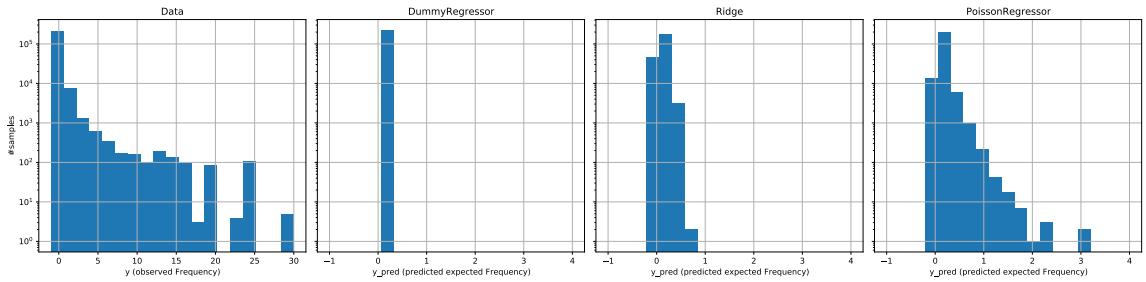
Figure 12.1: Predictions of insurance claim rates on the test set. (a) Data. (b) Constant predictor. (c) Linear regression. (d) Poisson regression. Generated by poisson\_regression\_insurance.ipynb.

Equation (10.21). This gradient expression can be used inside SGD, or some other gradient method, in the obvious way.

The Hessian is given by

\[\mathbf{H} = \frac{\partial^2}{\partial \mathbf{w} \partial \mathbf{w}^\mathrm{T}} \mathrm{NLL}(\mathbf{w}) = -\sum\_{n=1}^N \frac{\partial g\_n}{\partial \mathbf{w}^\mathrm{T}} \tag{12.32}\]

where

\[\frac{\partial \mathbf{g}\_n}{\partial \mathbf{w}^\mathsf{T}} = \frac{\partial \mathbf{g}\_n}{\partial \mu\_n} \frac{\partial \mu\_n}{\partial \mathbf{w}^\mathsf{T}} = -x\_n f'(\mathbf{w}^\mathsf{T} x\_n) \mathbf{x}\_n^\mathsf{T} \tag{12.33}\]

Hence

\[\mathbf{H} = \sum\_{n=1}^{N} f'(\eta\_n) \mathbf{x}\_n \mathbf{z}\_n^\top \tag{12.34}\]

For example, in the case of logistic regression, f(◁n) = ε(◁n), and f↗ (◁n) = ε(◁n)(1 ↑ ε(◁n)), so we recover Equation (10.23). In general, we see that the Hessian is positive definite, since f↗ (◁n) > 0; hence the negative log likelihood is convex, so the MLE for a GLM is unique (assuming f(◁n) > 0 for all n).

Based on the above results, we can fit GLMs using gradient based solvers in a manner that is very similar to how we fit logistic regression models.

12.5 Worked example: predicting insurance claims

In this section, we give an example of predicting insurance claims using linear and Poisson regression.2. The goal is to predict the expected number of insurance claims per year following car accidents. The dataset consists of 678k examples with 9 features, such as driver age, vehicle age, vehicle power,

^2. This example is from https://scikit-learn.org/stable/auto\_examples/linear\_model/plot\poisson\ regression\_non\_normal\_loss.html

Name	MSE	MAE	Deviance
Dummy	0.564	0.189	0.625
Ridge	0.560	0.177	0.601
Poisson	0.560	0.186	0.594

Table 12.1: Performance metrics on the test set. MSE = mean squared error. MAE = mean absolute error. Deviance = Poisson deviance.

etc. The target is the frequency of claims, which is the number of claims per policy divided by the exposure (i.e., the duration of the policy in years).

We plot the test set in Figure 12.1(a). We see that for 94% of the policies, no claims are made, so the data has lots of 0s, as is typical for count and rate data. The average frequency of claims is 10%. This can be converted into a dummy model, which always predicts this constant. This results in the predictions shown in Figure 12.1(b). The goal is to do better than this.

A simple approach is to use linear regression, combined with some simple feature engineering (binning the continuous values, and one-hot encoding the categoricals). (We use a small amount of ω² regularization, so technically this is ridge regression.) This gives the results shown in Figure 12.1(c). This is better than the baseline, but still not very good. In particular, it can predict negative outcomes, and fails to capture the long tail.

We can do better using Poisson regression, using the same features but a log link function. The results are shown in Figure 12.1(d). We see that predictions are much better.

An interesting question is how to quantify performance in this kind of problem. If we use mean squared error, or mean absolute error, we may conclude from Table 12.1 that ridge regression is better than Poisson regression, but this is clearly not true, as shown in Figure 12.1. Instead it is more common to measure performance using the deviance, which is defined as

\[D(\mathcal{y}, \hat{\mu}) = 2 \sum\_{i} \left( \log p(y\_i | \mu\_i^\*) - \log p(y\_i | \mu\_i) \right) \tag{12.35}\]

where µⁱ is the predicted parameters for the i’th example (based on the input features xⁱ and the training set D), and µ^{↓ i} is the optimal parameter estimated by fitting the model just to the true output yi. (This is the so-called saturated model, that perfectly fits the test set.) In the case of Poisson regression, we have µ^{↓ i} = yi. Hence

\[D(\boldsymbol{y}, \mu) = 2 \sum\_{i} \left[ (y\_i \log y\_i - y\_i - \log(y\_i!)) - (y\_i \log \hat{\mu}\_i - \hat{\mu}\_i - \log(y\_i!)) \right] \tag{12.36}\]

\[=2\sum\_{i}\left[\left(y\_i\log\frac{y\_i}{\hat{\mu}\_i}+\hat{\mu}\_i-y\_i\right)\right]\tag{12.37}\]

By this metric, the Poisson model is clearly better (see last column of Table 12.1).

We can also compute a calibration plot, which plots the actual frequency vs the predicted frequency. To compute this, we bin the predictions into intervals, and then count the empirical frequency of claims for all examples whose predicted frequency falls into that bin. The results are shown in Figure 12.2. We see that the constant baseline is well calibrated, but of course it is not very accurate. The ridge model is miscalibrated in the low frequency regime. In particular, it

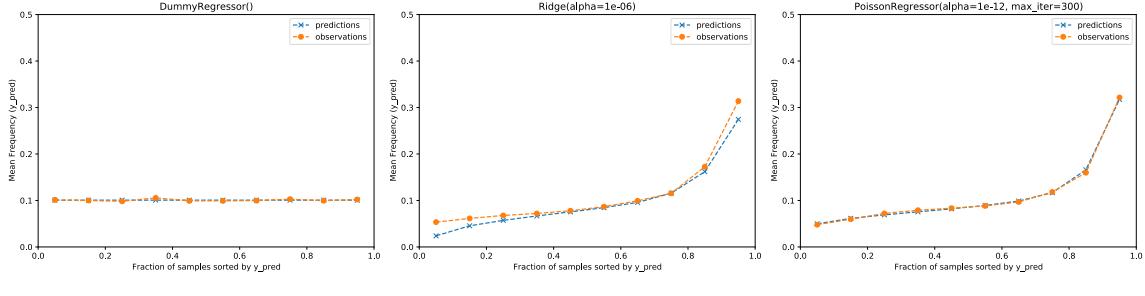
Figure 12.2: Calibration plot for insurance claims prediction. Generated by poisson\_regression\_insurance.ipynb.

underestimates the total number of claims in the test set to be 10,693, whereas the truth is 11,935. The Poisson model is better calibrated (i.e., when it predicts examples will have a high claim rate, they do in fact have a high claim rate), and it predicts the total number of claims to be 11,930.