Regression Modeling Strategies

Chapter 1 ~ 9

Author

Frank E. Harrell, Jr.

Springer Series in Statistics

Frank E. Harrell, Jr.

Regression Modeling Strategies

With Applications to Linear Models, Logistic and Ordinal Regression, and Survival Analysis

Second Edition

Springer Series in Statistics

Advisors: P. Bickel, P. Diggle, S.E. Feinberg, U. Gather, I. Olkin, S. Zeger

More information about this series at http://www.springer.com/series/692

Frank E. Harrell, Jr.

Regression Modeling Strategies

With Applications to Linear Models, Logistic and Ordinal Regression, and Survival Analysis

Second Edition

Frank E. Harrell, Jr. Department of Biostatistics School of Medicine Vanderbilt University Nashville, TN, USA

ISSN 0172-7397 ISSN 2197-568X (electronic) Springer Series in Statistics ISBN 978-3-319-19424-0 ISBN 978-3-319-19425-7 (eBook) DOI 10.1007/978-3-319-19425-7

Library of Congress Control Number: 2015942921

Springer Cham Heidelberg New York Dordrecht London

This work is subject to copyright. All rights are reserved by the Publisher, whether the whole or part of the material is concerned, specifically the rights of translation, reprinting, reuse of illustrations, recitation, broadcasting, reproduction on microfilms or in any other physical way, and transmission or information storage and retrieval, electronic adaptation, computer software, or by similar or dissimilar methodology now known or hereafter developed.

The use of general descriptive names, registered names, trademarks, service marks, etc. in this publication does not imply, even in the absence of a specific statement, that such names are exempt from the relevant protective laws and regulations and therefore free for general use.

The publisher, the authors and the editors are safe to assume that the advice and information in this book are believed to be true and accurate at the date of publication. Neither the publisher nor the authors or the editors give a warranty, express or implied, with respect to the material contained herein or for any errors or omissions that may have been made.

Printed on acid-free paper

Springer International Publishing AG Switzerland is part of Springer Science+Business Media (www. springer.com)

To the memories of Frank E. Harrell, Sr., Richard Jackson, L. Richard Smith, John Burdeshaw, and Todd Nick, and with appreciation to Liana and Charlotte Harrell, two high school math teachers: Carolyn Wailes (n´ee Gaston) and Floyd Christian, two college professors: David Hurst (who advised me to choose the field of biostatistics) and Doug Stocks, and my graduate advisor P. K. Sen.

Preface

There are many books that are excellent sources of knowledge about individual statistical tools (survival models, general linear models, etc.), but the art of data analysis is about choosing and using multiple tools. In the words of Chatfield [100, p. 420] “. . . students typically know the technical details of regression for example, but not necessarily when and how to apply it. This argues the need for a better balance in the literature and in statistical teaching between techniques and problem solving strategies.” Whether analyzing risk factors, adjusting for biases in observational studies, or developing predictive models, there are common problems that few regression texts address. For example, there are missing data in the majority of datasets one is likely to encounter (other than those used in textbooks!) but most regression texts do not include methods for dealing with such data effectively, and most texts on missing data do not cover regression modeling.

This book links standard regression modeling approaches with

methods for relaxing linearity assumptions that still allow one to easily obtain predictions and confidence limits for future observations, and to do formal hypothesis tests,
non-additive modeling approaches not requiring the assumption that interactions are always linear × linear,
methods for imputing missing data and for penalizing variances for incomplete data,
methods for handling large numbers of predictors without resorting to problematic stepwise variable selection techniques,
data reduction methods (unsupervised learning methods, some of which are based on multivariate psychometric techniques too seldom used in statistics) that help with the problem of “too many variables to analyze and not enough observations” as well as making the model more interpretable when there are predictor variables containing overlapping information,
methods for quantifying predictive accuracy of a fitted model,
powerful model validation techniques based on the bootstrap that allow the analyst to estimate predictive accuracy nearly unbiasedly without holding back data from the model development process, and
graphical methods for understanding complex models.

On the last point, this text has special emphasis on what could be called “presentation graphics for fitted models” to help make regression analyses more palatable to non-statisticians. For example, nomograms have long been used to make equations portable, but they are not drawn routinely because doing so is very labor-intensive. An R function called nomogram in the package described below draws nomograms from a regression fit, and these diagrams can be used to communicate modeling results as well as to obtain predicted values manually even in the presence of complex variable transformations.

Most of the methods in this text apply to all regression models, but special emphasis is given to some of the most popular ones: multiple regression using least squares and its generalized least squares extension for serial (repeated measurement) data, the binary logistic model, models for ordinal responses, parametric survival regression models, and the Cox semiparametric survival model. There is also a chapter on nonparametric transform-both-sides regression. Emphasis is given to detailed case studies for these methods as well as for data reduction, imputation, model simplification, and other tasks. Except for the case study on survival of Titanic passengers, all examples are from biomedical research. However, the methods presented here have broad application to other areas including economics, epidemiology, sociology, psychology, engineering, and predicting consumer behavior and other business outcomes.

This text is intended for Masters or PhD level graduate students who have had a general introductory probability and statistics course and who are well versed in ordinary multiple regression and intermediate algebra. The book is also intended to serve as a reference for data analysts and statistical methodologists. Readers without a strong background in applied statistics may wish to first study one of the many introductory applied statistics and regression texts that are available. The author’s course notes Biostatistics for Biomedical Research on the text’s web site covers basic regression and many other topics. The paper by Nick and Hardin [476] also provides a good introduction to multivariable modeling and interpretation. There are many excellent intermediate level texts on regression analysis. One of them is by Fox, which also has a companion software-based text [200, 201]. For readers interested in medical or epidemiologic research, Steyerberg’s excellent text Clinical Prediction Models [586] is an ideal companion for Regression Modeling Strategies. Steyerberg’s book provides further explanations, examples, and simulations of many of the methods presented here. And no text on regression modeling should fail to mention the seminal work of John Nelder [450].

The overall philosophy of this book is summarized by the following statements.

Satisfaction of model assumptions improves precision and increases statistical power.
It is more productive to make a model fit step by step (e.g., transformation estimation) than to postulate a simple model and find out what went wrong.
Graphical methods should be married to formal inference.
Overfitting occurs frequently, so data reduction and model validation are important.
In most research projects, the cost of data collection far outweighs the cost of data analysis, so it is important to use the most efficient and accurate modeling techniques, to avoid categorizing continuous variables, and to not remove data from the estimation sample just to be able to validate the model.
The bootstrap is a breakthrough for statistical modeling, and the analyst should use it for many steps of the modeling strategy, including derivation of distribution-free confidence intervals and estimation of optimism in model fit that takes into account variations caused by the modeling strategy.
Imputation of missing data is better than discarding incomplete observations.
Variance often dominates bias, so biased methods such as penalized maximum likelihood estimation yield models that have a greater chance of accurately predicting future observations.
Software without multiple facilities for assessing and fixing model fit may only seem to be user-friendly.
Carefully fitting an improper model is better than badly fitting (and overfitting) a well-chosen one.
Methods that work for all types of regression models are the most valuable.
Using the data to guide the data analysis is almost as dangerous as not doing so.
There are benefits to modeling by deciding how many degrees of freedom (i.e., number of regression parameters) can be “spent,” deciding where they should be spent, and then spending them.

On the last point, the author believes that significance tests and P-values are problematic, especially when making modeling decisions. Judging by the increased emphasis on confidence intervals in scientific journals there is reason to believe that hypothesis testing is gradually being de-emphasized. Yet the reader will notice that this text contains many P-values. How does that make sense when, for example, the text recommends against simplifying a model when a test of linearity is not significant? First, some readers may wish to emphasize hypothesis testing in general, and some hypotheses have special interest, such as in pharmacology where one may be interested in whether the effect of a drug is linear in log dose. Second, many of the more interesting hypothesis tests in the text are tests of complexity (nonlinearity, interaction) of the overall model. Null hypotheses of linearity of effects in particular are frequently rejected, providing formal evidence that the analyst’s investment of time to use more than simple statistical models was warranted.

The rapid development of Bayesian modeling methods and rise in their use is exciting. Full Bayesian modeling greatly reduces the need for the approximations made for confidence intervals and distributions of test statistics, and Bayesian methods formalize the still rather ad hoc frequentist approach to penalized maximum likelihood estimation by using skeptical prior distributions to obtain well-defined posterior distributions that automatically deal with shrinkage. The Bayesian approach also provides a formal mechanism for incorporating information external to the data. Although Bayesian methods are beyond the scope of this text, the text is Bayesian in spirit by emphasizing the careful use of subject matter expertise while building statistical models.

The text emphasizes predictive modeling, but as discussed in Chapter 1, developing good predictions goes hand in hand with accurate estimation of effects and with hypothesis testing (when appropriate). Besides emphasis on multivariable modeling, the text includes a Chapter 17 introducing survival analysis and methods for analyzing various types of single and multiple events. This book does not provide examples of analyses of one common type of response variable, namely, cost and related measures of resource consumption. However, least squares modeling presented in Chapter 15.1, the robust rank-based methods presented in Chapters 13, 15, and 20, and the transform-both-sides regression models discussed in Chapter 16 are very applicable and robust for modeling economic outcomes. See [167] and [260] for example analyses of such dependent variables using, respectively, the Cox model and nonparametric additive regression. The central Web site for this book (see the Appendix) has much more material on the use of the Cox model for analyzing costs.

This text does not address some important study design issues that if not respected can doom a predictive modeling or estimation project to failure. See Laupacis, Sekar, and Stiell [378] for a list of some of these issues.

Heavy use is made of the S language used by R. R is the focus because it is an elegant object-oriented system in which it is easy to implement new statistical ideas. Many R users around the world have done so, and their work has benefited many of the procedures described here. R also has a uniform syntax for specifying statistical models (with respect to categorical predictors, interactions, etc.), no matter which type of model is being fitted [96].

The free, open-source statistical software system R has been adopted by analysts and research statisticians worldwide. Its capabilities are growing exponentially because of the involvement of an ever-growing community of statisticians who are adding new tools to the base R system through contributed packages. All of the functions used in this text are available in R. See the book’s Web site for updated information about software availability.

Readers who don’t use R or any other statistical software environment will still find the statistical methods and case studies in this text useful, and it is hoped that the code that is presented will make the statistical methods more concrete. At the very least, the code demonstrates that all of the methods presented in the text are feasible.

This text does not teach analysts how to use R. For that, the reader may wish to see reading recommendations on www.r-project.org as well as Venables and Ripley [635] (which is also an excellent companion to this text) and the many other excellent texts on R. See the Appendix for more information.

In addition to powerful features that are built into R, this text uses a package of freely available R functions called rms written by the author. rms tracks modeling details related to the expanded X or design matrix. It is a series of over 200 functions for model fitting, testing, estimation, validation, graphics, prediction, and typesetting by storing enhanced model design attributes in the fit. rms includes functions for least squares and penalized least squares multiple regression modeling in addition to functions for binary and ordinal regression, generalized least squares for analyzing serial data, quantile regression, and survival analysis that are emphasized in this text. Other freely available miscellaneous R functions used in the text are found in the Hmisc package also written by the author. Functions in Hmisc include facilities for data reduction, imputation, power and sample size calculation, advanced table making, recoding variables, importing and inspecting data, and general graphics. Consult the Appendix for information on obtaining Hmisc and rms.

The author and his colleagues have written SAS macros for fitting restricted cubic splines and for other basic operations. See the Appendix for more information. It is unfair not to mention some excellent capabilities of other statistical packages such as Stata (which has also been extended to provide regression splines and other modeling tools), but the extendability and graphics of R makes it especially attractive for all aspects of the comprehensive modeling strategy presented in this book.

Portions of Chapters 4 and 20 were published as reference [269]. Some of Chapter 13 was published as reference [272].

The author may be contacted by electronic mail at f.harrell@ vanderbilt.edu and would appreciate being informed of unclear points, errors, and omissions in this book. Suggestions for improvements and for future topics are also welcome. As described in the Web site, instructors may contact the author to obtain copies of quizzes and extra assignments (both with answers) related to much of the material in the earlier chapters, and to obtain full solutions (with graphical output) to the majority of assignments in the text.

Major changes since the first edition include the following:

1. Creation of a now mature R package, rms, that replaces and greatly extends the Design library used in the first edition
1. Conversion of all of the book’s code to R
1. Conversion of the book source into knitr [677] reproducible documents
1. All code from the text is executable and is on the web site
1. Use of color graphics and use of the ggplot2 graphics package [667]
1. Scanned images were re-drawn
1. New text about problems with dichotomization of continuous variables and with classification (as opposed to prediction)
1. Expanded material on multiple imputation and predictive mean matching and emphasis on multiple imputation (using the Hmisc aregImpute function) instead of single imputation
1. Addition of redundancy analysis
1. Added a new section in Chapter 5 on bootstrap confidence intervals for rankings of predictors
1. Replacement of the U.S. presidential election data with analyses of a new diabetes dataset from NHANES using ordinal and quantile regression
1. More emphasis on semiparametric ordinal regression models for continuous Y , as direct competitors of ordinary multiple regression, with a detailed case study
1. A new chapter on generalized least squares for analysis of serial response data
1. The case study in imputation and data reduction was completely reworked and now focuses only on data reduction, with the addition of sparse principal components
1. More information about indexes of predictive accuracy
1. Augmentation of the chapter on maximum likelihood to include more flexible ways of testing contrasts as well as new methods for obtaining simultaneous confidence intervals
1. Binary logistic regression case study 1 was completely re-worked, now providing examples of model selection and model approximation accuracy
1. Single imputation was dropped from binary logistic case study 2
1. The case study in transform-both-sides regression modeling has been reworked using simulated data where true transformations are known, and a new example of the smearing estimator was added
1. Addition of 225 references, most of them published 2001–2014
1. New guidance on minimum sample sizes needed by some of the models
1. De-emphasis of bootstrap bumping [610] for obtaining simultaneous confidence regions, in favor of a general multiplicity approach [307].

Acknowledgments

A good deal of the writing of the first edition of this book was done during my 17 years on the faculty of Duke University. I wish to thank my close colleague Kerry Lee for providing many valuable ideas, fruitful collaborations, and well-organized lecture notes from which I have greatly benefited over the past years. Terry Therneau of Mayo Clinic has given me many of his wonderful ideas for many years, and has written state-of-the-art R software for survival analysis that forms the core of survival analysis software in my rms package. Michael Symons of the Department of Biostatistics of the University of North Carolina at Chapel Hill and Timothy Morgan of the Division of Public Health Sciences at Wake Forest University School of Medicine also provided course materials, some of which motivated portions of this text. My former clinical colleagues in the Cardiology Division at Duke University, Robert Califf, Phillip Harris, Mark Hlatky, Dan Mark, David Pryor, and Robert Rosati, for many years provided valuable motivation, feedback, and ideas through our interaction on clinical problems. Besides Kerry Lee, statistical colleagues L. Richard Smith, Lawrence Muhlbaier, and Elizabeth DeLong clarified my thinking and gave me new ideas on numerous occasions. Charlotte Nelson and Carlos Alzola frequently helped me debug S routines when they thought they were just analyzing data.

Former students Bercedis Peterson, James Herndon, Robert McMahon, and Yuan-Li Shen have provided many insights into logistic and survival modeling. Associations with Doug Wagner and William Knaus of the University of Virginia, Ken Offord of Mayo Clinic, David Naftel of the University of Alabama in Birmingham, Phil Miller of Washington University, and Phil Goodman of the University of Nevada Reno have provided many valuable ideas and motivations for this work, as have Michael Schemper of Vienna University, Janez Stare of Ljubljana University, Slovenia, Ewout Steyerberg of Erasmus University, Rotterdam, Karel Moons of Utrecht University, and Drew Levy of Genentech. Richard Goldstein, along with several anonymous reviewers, provided many helpful criticisms of a previous version of this manuscript that resulted in significant improvements, and critical reading by Bob Edson (VA Cooperative Studies Program, Palo Alto) resulted in many error corrections. Thanks to Brian Ripley of the University of Oxford for providing many helpful software tools and statistical insights that greatly aided in the production of this book, and to Bill Venables of CSIRO Australia for wisdom, both statistical and otherwise. This work would also not have been possible without the S environment developed by Rick Becker, John Chambers, Allan Wilks, and the R language developed by Ross Ihaka and Robert Gentleman.

Work for the second edition was done in the excellent academic environment of Vanderbilt University, where biostatistical and biomedical colleagues and graduate students provided new insights and stimulating discussions. Thanks to Nick Cox, Durham University, UK, who provided from his careful reading of the first edition a very large number of improvements and corrections that were incorporated into the second. Four anonymous reviewers of the second edition also made numerous suggestions that improved the text.

July 2015

Nashville, TN, USA Frank E. Harrell, Jr.

			Typographical Conventions . xxv
1		Introduction		1
	1.1		Hypothesis Testing, Estimation, and Prediction	1
	1.2		Examples of Uses of Predictive Multivariable Modeling	3
	1.3		Prediction vs. Classification	4
	1.4		Planning for Modeling	6
		1.4.1	Emphasizing Continuous Variables	8
	1.5		Choice of the Model	8
	1.6		Further Reading .	11
2			General Aspects of Fitting Regression Models .	13
	2.1		Notation for Multivariable Regression Models .	13
	2.2		Model Formulations .	14
	2.3		Interpreting Model Parameters .	15
		2.3.1	Nominal Predictors .	16
		2.3.2	Interactions.	16
		2.3.3	Example: Inference for a Simple Model .	17
	2.4		Relaxing Linearity Assumption for Continuous Predictors . .	18
		2.4.1	Avoiding Categorization .	18
		2.4.2	Simple Nonlinear Terms .	21
		2.4.3	Splines for Estimating Shape of Regression
			Function and Determining Predictor
			Transformations.	22
		2.4.4	Cubic Spline Functions.	23
		2.4.5	Restricted Cubic Splines .	24
		2.4.6	Choosing Number and Position of Knots .	26
		2.4.7	Nonparametric Regression .	28
		2.4.8	Advantages of Regression Splines over
			Other Methods.	30

	2.5	Recursive Partitioning: Tree-Based Models.	30
	2.6	Multiple Degree of Freedom Tests of Association .	31
	2.7	Assessment of Model Fit .	33
		2.7.1 Regression Assumptions .	33
		2.7.2 Modeling and Testing Complex Interactions .	36
		2.7.3 Fitting Ordinal Predictors .	38
		2.7.4 Distributional Assumptions .	39
	2.8	Further Reading .	40
	2.9	Problems .	42
3		Missing Data .	45
	3.1	Types of Missing Data .	45
	3.2	Prelude to Modeling .	46
	3.3	Missing Values for Different Types of Response Variables .	47
	3.4	Problems with Simple Alternatives to Imputation .	47
	3.5	Strategies for Developing an Imputation Model .	49
	3.6	Single Conditional Mean Imputation .	52
	3.7	Predictive Mean Matching .	52
	3.8	Multiple Imputation .	53
		3.8.1 The aregImpute and Other Chained Equations
		Approaches .	55
	3.9	Diagnostics .	56
	3.10	Summary and Rough Guidelines.	56
	3.11	Further Reading .	58
	3.12	Problems .	59
4		Multivariable Modeling Strategies .	63
	4.1	Prespecification of Predictor Complexity Without
		Later Simplification .	64
	4.2	Checking Assumptions of Multiple Predictors
		Simultaneously .	67
	4.3	Variable Selection .	67
	4.4	Sample Size, Overfitting, and Limits on Number
		of Predictors .	72
	4.5	Shrinkage .	75
	4.6	Collinearity .	78
	4.7	Data Reduction .	79
		4.7.1 Redundancy Analysis .	80
		4.7.2 Variable Clustering .	81
		4.7.3 Transformation and Scaling Variables Without
		Using Y .	81
		4.7.4 Simultaneous Transformation and Imputation .	83
		4.7.5 Simple Scoring of Variable Clusters .	85
		4.7.6 Simplifying Cluster Scores .	87
		4.7.7 How Much Data Reduction Is Necessary? .	87

	4.8	Other Approaches to Predictive Modeling .	89
	4.9	Overly Influential Observations.	90
	4.10	Comparing Two Models .	92
	4.11	Improving the Practice of Multivariable Prediction .	94
	4.12	Summary: Possible Modeling Strategies .	94
		4.12.1 Developing Predictive Models .	95
		4.12.2 Developing Models for Effect Estimation .	98
		4.12.3 Developing Models for Hypothesis Testing .	99
	4.13	Further Reading . 100
	4.14	Problems . 102
5		Describing, Resampling, Validating, and Simplifying
		the Model . 103
	5.1	Describing the Fitted Model . 103
		5.1.1 Interpreting Effects . 103
		5.1.2 Indexes of Model Performance . 104
	5.2	The Bootstrap . 106
	5.3	Model Validation . 109
		5.3.1 Introduction . 109
		5.3.2 Which Quantities Should Be Used in Validation? . 110
		5.3.3 Data-Splitting . 111
		5.3.4 Improvements on Data-Splitting: Resampling . 112
		5.3.5 Validation Using the Bootstrap . 114
	5.4	Bootstrapping Ranks of Predictors. 117
	5.5	Simplifying the Final Model by Approximating It. 118
		5.5.1 Difficulties Using Full Models . 118
		5.5.2 Approximating the Full Model . 119
	5.6	Further Reading . 121
	5.7	Problem . 124
6		R Software . 127
	6.1	The R Modeling Language . 128
	6.2	User-Contributed Functions. 129
	6.3	The rms Package . 130
	6.4	Other Functions . 141
	6.5	Further Reading . 142
7		Modeling Longitudinal Responses using Generalized
		Least Squares . 143
	7.1	Notation and Data Setup . 143
	7.2	Model Specification for Effects on E(Y ) . 144
	7.3	Modeling Within-Subject Dependence . 144
	7.4	Parameter Estimation Procedure . 147
	7.5	Common Correlation Structures . 147
	7.6	Checking Model Fit. 148

	7.7	Sample Size Considerations . 148
	7.8	R Software . 149
	7.9	Case Study . 149
		7.9.1 Graphical Exploration of Data . 150
		7.9.2 Using Generalized Least Squares . 151
	7.10	Further Reading . 158
8		Case Study in Data Reduction. 161
	8.1	Data . 161
	8.2	How Many Parameters Can Be Estimated? . 164
	8.3	Redundancy Analysis . 164
	8.4	Variable Clustering . 166
	8.5	Transformation and Single Imputation Using transcan. 167
	8.6	Data Reduction Using Principal Components . 170
		8.6.1 Sparse Principal Components . 175
	8.7	Transformation Using Nonparametric Smoothers . 176
	8.8	Further Reading . 177
	8.9	Problems . 178
9		Overview of Maximum Likelihood Estimation . 181
	9.1	General Notions—Simple Cases . 181
	9.2	Hypothesis Tests . 185
		9.2.1 Likelihood Ratio Test . 185
		9.2.2 Wald Test . 186
		9.2.3 Score Test . 186
		9.2.4 Normal Distribution—One Sample . 187
	9.3	General Case . 188
		9.3.1 Global Test Statistics . 189
		9.3.2 Testing a Subset of the Parameters . 190
		9.3.3 Tests Based on Contrasts. 192
		9.3.4 Which Test Statistics to Use When . 193
		9.3.5 Example: Binomial—Comparing Two
		Proportions. 194
	9.4	Iterative ML Estimation . 195
	9.5	Robust Estimation of the Covariance Matrix . 196
	9.6	Wald, Score, and Likelihood-Based Confidence Intervals	. 198
		9.6.1 Simultaneous Wald Confidence Regions . 199
	9.7	Bootstrap Confidence Regions. 199
	9.8	Further Use of the Log Likelihood . 203
		9.8.1 Rating Two Models, Penalizing for Complexity	. 203
		9.8.2 Testing Whether One Model Is Better
		than Another . 204
		9.8.3 Unitless Index of Predictive Ability . 205
		9.8.4 Unitless Index of Adequacy of a Subset
		of Predictors. 207
	9.9	Weighted Maximum Likelihood Estimation . 208
	9.10	Penalized Maximum Likelihood Estimation . 209

	9.11	Further Reading . 213
	9.12	Problems . 216

10		Binary Logistic Regression. 219
	10.1	Model. 219
		10.1.1 Model Assumptions and Interpretation
		of Parameters . 221
		10.1.2 Odds Ratio, Risk Ratio, and Risk Difference . 224
		10.1.3 Detailed Example . 225
		10.1.4 Design Formulations . 230
	10.2	Estimation . 231
		10.2.1 Maximum Likelihood Estimates . 231
		10.2.2 Estimation of Odds Ratios and Probabilities . 232
		10.2.3 Minimum Sample Size Requirement . 233
	10.3	Test Statistics. 234
	10.4	Residuals . 235
	10.5	Assessment of Model Fit . 236
	10.6	Collinearity . 255
	10.7	Overly Influential Observations. 255
	10.8 10.9	Quantifying Predictive Ability . 256 Validating the Fitted Model . 259
		10.10 Describing the Fitted Model . 264
	10.11	R Functions . 269
		10.12 Further Reading . 271
		10.13 Problems . 273

11		Binary Logistic Regression Case Study 1 . 275
	11.1	Overview . 275
	11.2	Background. 275
	11.3	Data Transformations and Single Imputation . 276
	11.4	Regression on Original Variables, Principal Components
		and Pretransformations . 277
	11.5	Description of Fitted Model. 278
	11.6	Backwards Step-Down . 280
	11.7	Model Approximation . 287
12		Logistic Model Case Study 2: Survival of Titanic
		Passengers . 291
	12.1	Descriptive Statistics. 291
	12.2	Exploring Trends with Nonparametric Regression . 294
	12.3	Binary Logistic Model With Casewise Deletion
		of Missing Values . 296
	12.4	Examining Missing Data Patterns . 302
	12.5	Multiple Imputation . 304
	12.6	Summarizing the Fitted Model . 307

13		Ordinal Logistic Regression . 311
	13.1	Background. 311
	13.2	Ordinality Assumption . 312
	13.3	Proportional Odds Model. 313
		13.3.1 Model . 313
		13.3.2 Assumptions and Interpretation of Parameters . 313
		13.3.3 Estimation . 314
		13.3.4 Residuals. 314
		13.3.5 Assessment of Model Fit . 315
		13.3.6 Quantifying Predictive Ability . 318
		13.3.7 Describing the Fitted Model . 318
		13.3.8 Validating the Fitted Model . 318
		13.3.9 R Functions. 319
	13.4	Continuation Ratio Model . 319
		13.4.1 Model . 319
		13.4.2 Assumptions and Interpretation of Parameters . 320
		13.4.3 Estimation . 320
		13.4.4 Residuals. 321
		13.4.5 Assessment of Model Fit . 321
		13.4.6 Extended CR Model . 321
		13.4.7 Role of Penalization in Extended CR Model . 322
		13.4.8 Validating the Fitted Model . 322
		13.4.9 R Functions. 323
	13.5	Further Reading . 324
	13.6	Problems . 324
14		Case Study in Ordinal Regression, Data Reduction,
		and Penalization . 327
	14.1	Response Variable . 328
	14.2	Variable Clustering . 329
	14.3	Developing Cluster Summary Scores . 330
	14.4	Assessing Ordinality of Y for each X, and Unadjusted
		Checking of PO and CR Assumptions . 333
	14.5	A Tentative Full Proportional Odds Model . 333
	14.6	Residual Plots . 336
	14.7	Graphical Assessment of Fit of CR Model . 338
	14.8	Extended Continuation Ratio Model . 340
	14.9	Penalized Estimation . 342
		14.10 Using Approximations to Simplify the Model . 348
		14.11 Validating the Model . 353
		14.12 Summary . 355
		14.13 Further Reading . 356
		14.14 Problems . 357

15	Regression Models for Continuous Y and Case Study
		in Ordinal Regression. 359
	15.1	The Linear Model . 359
	15.2	Quantile Regression. 360
	15.3	Ordinal Regression Models for Continuous Y . 361
		15.3.1 Minimum Sample Size Requirement . 363
	15.4	Comparison of Assumptions of Various Models . 364
	15.5	Dataset and Descriptive Statistics . 365
		15.5.1 Checking Assumptions of OLS and Other Models. 368
	15.6	Ordinal Regression Applied to HbA1c . 370
		15.6.1 Checking Fit for Various Models Using Age . 370
		15.6.2 Examination of BMI . 374
		15.6.3 Consideration of All Body Size Measurements. 375
16		Transform-Both-Sides Regression . 389
	16.1	Background. 389
	16.2	Generalized Additive Models. 390
	16.3	Nonparametric Estimation of Y -Transformation . 390
	16.4	Obtaining Estimates on the Original Scale . 391
	16.5	R Functions . 392
	16.6	Case Study . 393
17		Introduction to Survival Analysis . 399
	17.1	Background. 399
	17.2	Censoring, Delayed Entry, and Truncation . 401
	17.3	Notation, Survival, and Hazard Functions . 402
	17.4	Homogeneous Failure Time Distributions . 407
	17.5	Nonparametric Estimation of S and Λ . 409
		17.5.1 Kaplan–Meier Estimator . 409
		17.5.2 Altschuler–Nelson Estimator . 413
	17.6	Analysis of Multiple Endpoints . 413
		17.6.1 Competing Risks . 414
		17.6.2 Competing Dependent Risks . 414

		17.6.3 State Transitions and Multiple Types of Nonfatal Events . 416
		17.6.4 Joint Analysis of Time and Severity of an Event. 417
		17.6.5 Analysis of Multiple Events. 417
	17.7	R Functions . 418
	17.8	Further Reading . 420
	17.9	Problems . 421
18		Parametric Survival Models . 423
	18.1	Homogeneous Models (No Predictors) . 423
		18.1.1 Specific Models . 423
		18.1.2 Estimation . 424
		18.1.3 Assessment of Model Fit . 426

	18.2	Parametric Proportional Hazards Models . 427
		18.2.1 Model . 427
		18.2.2 Model Assumptions and Interpretation
		of Parameters . 428
		18.2.3 Hazard Ratio, Risk Ratio, and Risk Difference	. 430
		18.2.4 Specific Models . 431
		18.2.5 Estimation . 432
		18.2.6 Assessment of Model Fit . 434
	18.3	Accelerated Failure Time Models . 436
		18.3.1 Model . 436
		18.3.2 Model Assumptions and Interpretation
		of Parameters . 436
		18.3.3 Specific Models . 437
		18.3.4 Estimation . 438
		18.3.5 Residuals. 440
		18.3.6 Assessment of Model Fit . 440
		18.3.7 Validating the Fitted Model . 446
	18.4	Buckley–James Regression Model . 447
	18.5	Design Formulations . 447
	18.6	Test Statistics. 447
	18.7	Quantifying Predictive Ability . 447
	18.8	Time-Dependent Covariates. 447
	18.9	R Functions . 448
		18.10 Further Reading . 450
		18.11 Problems . 451

19		Case Study in Parametric Survival Modeling and Model
		Approximation . 453
	19.1	Descriptive Statistics. 453
	19.2	Checking Adequacy of Log-Normal Accelerated Failure
		Time Model . 458
	19.3	Summarizing the Fitted Model . 466
	19.4	Internal Validation of the Fitted Model Using
		the Bootstrap . 466
	19.5	Approximating the Full Model . 469
	19.6	Problems . 473
20		Cox Proportional Hazards Regression Model . 475
	20.1	Model. 475
		20.1.1 Preliminaries . 475
		20.1.2 Model Definition . 476
		20.1.3 Estimation of β . 476
		20.1.4 Model Assumptions and Interpretation
		of Parameters . 478
		20.1.5 Example . 478

		20.1.6 Design Formulations . 480
		20.1.7 Extending the Model by Stratification . 481
	20.2	Estimation of Survival Probability and Secondary
		Parameters . 483
	20.3	Sample Size Considerations . 486
	20.4	Test Statistics. 486
	20.5	Residuals . 487
	20.6	Assessment of Model Fit . 487 20.6.1 Regression Assumptions . 487
		20.6.2 Proportional Hazards Assumption . 494
	20.7	What to Do When PH Fails . 501
	20.8	Collinearity . 503
	20.9	Overly Influential Observations. 504
		20.10 Quantifying Predictive Ability . 504
		20.11 Validating the Fitted Model . 506
		20.11.1 Validation of Model Calibration . 506
		20.11.2 Validation of Discrimination and Other Statistical
		Indexes . 507
		20.12 Describing the Fitted Model . 509
	20.13	R Functions . 513
		20.14 Further Reading . 517
21		Case Study in Cox Regression . 521
	21.1	Choosing the Number of Parameters and Fitting
		the Model . 521
	21.2	Checking Proportional Hazards . 525
	21.3	Testing Interactions. 527
	21.4	Describing Predictor Effects . 527
	21.5	Validating the Model . 529
	21.6	Presenting the Model . 530
	21.7	Problems . 531
A	Datasets,	R Packages, and Internet Resources . 535
	References	. 539
Index		. 571

Typographical Conventions

Boxed numbers in the margins such as ¹ correspond to numbers at the end of chapters in sections named “Further Reading.” Bracketed numbers and numeric superscripts in the text refer to the bibliography, while alphabetic superscripts indicate footnotes.

R language commands and names of R functions and packages are set in typewriter font, as are most variable names.

R code blocks are set off with a shadowbox, and R output that is not directly using LATEX appears in a box that is framed on three sides.

In the S language upon which ^R is based, ^x ← ^y is read “^x gets the value of ^y.” The assignment operator ←, used in the text for aesthetic reasons (as are ≤ and ≥), is entered by the user as <-. Comments begin with #, subscripts use brackets ([ ]), and the missing value is denoted by NA (not available).

In ordinary text and mathematical expressions, [logical variable] and [logical expression] imply a value of 1 if the logical variable or expression is true, and 0 otherwise.

Chapter 1 Introduction

1.1 Hypothesis Testing, Estimation, and Prediction

Statistics comprises among other areas study design, hypothesis testing, estimation, and prediction. This text aims at the last area, by presenting methods that enable an analyst to develop models that will make accurate predictions of responses for future observations. Prediction could be considered a superset of hypothesis testing and estimation, so the methods presented here will also assist the analyst in those areas. It is worth pausing to explain how this is so.

In traditional hypothesis testing one often chooses a null hypothesis defined as the absence of some effect. For example, in testing whether a variable such as cholesterol is a risk factor for sudden death, one might test the null hypothesis that an increase in cholesterol does not increase the risk of death. Hypothesis testing can easily be done within the context of a statistical model, but a model is not required. When one only wishes to assess whether an effect is zero, P-values may be computed using permutation or rank (nonparametric) tests while making only minimal assumptions. But there are still reasons for preferring a model-based approach over techniques that only yield P-values.

1. Permutation and rank tests do not easily give rise to estimates of magnitudes of effects.
1. These tests cannot be readily extended to incorporate complexities such as cluster sampling or repeated measurements within subjects.
1. Once the analyst is familiar with a model, that model may be used to carry out many different statistical tests; there is no need to learn specific formulas to handle the special cases. The two-sample t-test is a special case of the ordinary multiple regression model having as its sole X variable a dummy variable indicating group membership. The Wilcoxon-Mann-Whitney test is a special case of the proportional odds ordinal logistic

^© Springer International Publishing Switzerland 2015

F.E. Harrell, Jr., Regression Modeling Strategies, Springer Series in Statistics, DOI 10.1007/978-3-319-19425-7 1

model.664 The analysis of variance (multiple group) test and the Kruskal– Wallis test can easily be obtained from these two regression models by using more than one dummy predictor variable.

Even without complexities such as repeated measurements, problems can arise when many hypotheses are to be tested. Testing too many hypotheses is related to fitting too many predictors in a regression model. One commonly hears the statement that “the dataset was too small to allow modeling, so we just did hypothesis tests.” It is unlikely that the resulting inferences would be reliable. If the sample size is insufficient for modeling it is often insufficient for tests or estimation. This is especially true when one desires to publish an estimate of the effect corresponding to the hypothesis yielding the smallest P-value. Ordinary point estimates are known to be badly biased when the quantity to be estimated was determined by “data dredging.” This can be remedied by the same kind of shrinkage used in multivariable modeling (Section 9.10).

Statistical estimation is usually model-based. For example, one might use a survival regression model to estimate the relative effect of increasing cholesterol from 200 to 250 mg/dl on the hazard of death. Variables other than cholesterol may also be in the regression model, to allow estimation of the effect of increasing cholesterol, holding other risk factors constant. But accurate estimation of the cholesterol effect will depend on how cholesterol as well as each of the adjustment variables is assumed to relate to the hazard of death. If linear relationships are incorrectly assumed, estimates will be inaccurate. Accurate estimation also depends on avoiding overfitting the adjustment variables. If the dataset contains 200 subjects, 30 of whom died, and if one adjusted for 15 “confounding” variables, the estimates would be “overadjusted” for the effects of the 15 variables, as some of their apparent effects would actually result from spurious associations with the response variable (time until death). The overadjustment would reduce the cholesterol effect. The resulting unreliability of estimates equals the degree to which the overall model fails to validate on an independent sample.

It is often useful to think of effect estimates as differences between two predicted values from a model. This way, one can account for nonlinearities and interactions. For example, if cholesterol is represented nonlinearly in a logistic regression model, predicted values on the “linear combination of X’s scale” are predicted log odds of an event. The increase in log odds from raising cholesterol from 200 to 250 mg/dl is the difference in predicted values, where cholesterol is set to 250 and then to 200, and all other variables are held constant. The point estimate of the 250:200 mg/dl odds ratio is the anti-log of this difference. If cholesterol is represented nonlinearly in the model, it does not matter how many terms in the model involve cholesterol as long as the overall predicted values are obtained.

Thus when one develops a reasonable multivariable predictive model, hypothesis testing and estimation of effects are byproducts of the fitted model. So predictive modeling is often desirable even when prediction is not the main goal.

1.2 Examples of Uses of Predictive Multivariable Modeling

There is an endless variety of uses for multivariable models. Predictive models have long been used in business to forecast financial performance and to model consumer purchasing and loan pay-back behavior. In ecology, regression models are used to predict the probability that a fish species will disappear from a lake. Survival models have been used to predict product life (e.g., time to burn-out of an mechanical part, time until saturation of a disposable diaper). Models are commonly used in discrimination litigation in an attempt to determine whether race or sex is used as the basis for hiring or promotion, after taking other personnel characteristics into account.

Multivariable models are used extensively in medicine, epidemiology, biostatistics, health services research, pharmaceutical research, and related fields. The author has worked primarily in these fields, so most of the examples in this text come from those areas. In medicine, two of the major areas of application are diagnosis and prognosis. There models are used to predict the probability that a certain type of patient will be shown to have a specific disease, or to predict the time course of an already diagnosed disease. In observational studies in which one desires to compare patient outcomes between two or more treatments, multivariable modeling is very important because of the biases caused by nonrandom treatment assignment. Here the simultaneous effects of several uncontrolled variables must be controlled (held constant mathematically if using a regression model) so that the effect of the factor of interest can be more purely estimated. A newer technique for more aggressively adjusting for nonrandom treatment assignment, the propensity score, 116, 530 provides yet another opportunity for multivariable modeling (see Section 10.1.4). The propensity score is merely the predicted value from a multivariable model where the response variable is the exposure or the treatment actually used. The estimated propensity score is then used in a second step as an adjustment variable in the model for the response of interest.

It is not widely recognized that multivariable modeling is extremely valuable even in well-designed randomized experiments. Such studies are often designed to make relative comparisons of two or more treatments, using odds ratios, hazard ratios, and other measures of relative effects. But to be able to estimate absolute effects one must develop a multivariable model of the response variable. This model can predict, for example, the probability that a patient on treatment A with characteristics X will survive five years, or it can predict the life expectancy for this patient. By making the same prediction for a patient on treatment B with the same characteristics, one can estimate the absolute difference in probabilities or life expectancies. This approach recognizes that low-risk patients must have less absolute benefit of treatment (lower change in outcome probability) than high-risk patients,351 a fact that has been ignored in many clinical trials. Another reason for multivariable modeling in randomized clinical trials is that when the basic response model is nonlinear (e.g., logistic, Cox, parametric survival models), the unadjusted estimate of the treatment effect is not correct if there is moderate heterogeneity of subjects, even with perfect balance of baseline characteristics across the treatment groups.a9, 24, 198, 588 So even when investigators are interested in simple comparisons of two groups’ responses, multivariable modeling can be advantageous and sometimes mandatory.

Cost-effectiveness analysis is becoming increasingly used in health care research, and the “effectiveness” (denominator of the cost-effectiveness ratio) is always a measure of absolute effectiveness. As absolute effectiveness varies dramatically with the risk profiles of subjects, it must be estimated for individual subjects using a multivariable model90, 344.

1.3 Prediction vs. Classification

For problems ranging from bioinformatics to marketing, many analysts desire to develop “classifiers” instead of developing predictive models. Consider an optimum case for classifier development, in which the response variable is binary, the two levels represent a sharp dichotomy with no gray zone (e.g., complete success vs. total failure with no possibility of a partial success), the user of the classifier is forced to make one of the two choices, the cost of misclassification is the same for every future observation, and the ratio of the cost of a false positive to that of a false negative equals the (often hidden) ratio implied by the analyst’s classification rule. Even if all of those conditions are met, classification is still inferior to probability modeling for driving the development of a predictive instrument or for estimation or hypothesis testing. It is far better to use the full information in the data to develop a probability model, then develop classification rules on the basis of estimated probabilities. At the least, this forces the analyst to use a proper accuracy score219 in finding or weighting data features.

When the dependent variable is ordinal or continuous, classification through forced up-front dichotomization in an attempt to simplify the problem results in arbitrariness and major information loss even when the optimum cut point

^a For example, unadjusted odds ratios from 2 ^× 2 tables are different from adjusted odds ratios when there is variation in subjects’ risk factors within each treatment group, even when the distribution of the risk factors is identical between the two groups.

(the median) is used. Dichtomizing the outcome at a different point may require a many-fold increase in sample size to make up for the lost information187. In the area of medical diagnosis, it is often the case that the disease is really on a continuum, and predicting the severity of disease (rather than just its presence or absence) will greatly increase power and precision, not to mention making the result less arbitrary.

It is important to note that two-group classification represents an artificial forced choice. It is not often the case that the user of the classifier needs to be limited to two possible actions. The best option for many subjects may be to refuse to make a decision or to obtain more data (e.g., order another medical diagnostic test). A gray zone can be helpful, and predictions include gray zones automatically.

Unlike prediction (e.g., of absolute risk), classification implicitly uses utility functions (also called loss or cost functions, e.g., cost of a false positive classification). Implicit utility functions are highly problematic. First, it is well known that the utility function depends on variables that are not predictive of outcome and are not collected (e.g., subjects’ preferences) that are available only at the decision point. Second, the approach assumes every subject has the same utility functionb. Third, the analyst presumptuously assumes that the subject’s utility coincides with his own.

Formal decision analysis uses subject-specific utilities and optimum predictions based on all available data62, 74, 183, 210, 219, 642c. It follows that receiver

^b Simple examples to the contrary are the less weight given to a false negative diagnosis of cancer in the elderly and the aversion of some subjects to surgery or chemotherapy.

^c To make an optimal decision you need to know all relevant data about an individual (used to estimate the probability of an outcome), and the utility (cost, loss function) of making each decision. Sensitivity and specificity do not provide this information. For example, if one estimated that the probability of a disease given age, sex, and symptoms is 0.1 and the “cost”of a false positive equaled the “cost” of a false negative, one would act as if the person does not have the disease. Given other utilities, one would make different decisions. If the utilities are unknown, one gives the best estimate of the probability of the outcome to the decision maker and let her incorporate her own unspoken utilities in making an optimum decision for her.

Besides the fact that cutoffs that are not individualized do not apply to individuals, only to groups, individual decision making does not utilize sensitivity and specificity. For an individual we can compute Prob(Y = 1|X = x); we don’t care about Prob(Y = 1|X>c), and an individual having X = x would be quite puzzled if she were given Prob(X>c|future unknown Y) when she already knows X = x so X is no longer a random variable.

Even when group decision making is needed, sensitivity and specificity can be bypassed. For mass marketing, for example, one can rank order individuals by the estimated probability of buying the product, to create a lift curve. This is then used to target the k most likely buyers where k is chosen to meet total program cost constraints.

operating characteristic curve (ROCd) analysis is misleading except for the special case of mass one-time group decision making with unknown utilities 1 (e.g., launching a flu vaccination program).

An analyst’s goal should be the development of the most accurate and reliable predictive model or the best model on which to base estimation or hypothesis testing. In the vast majority of cases, classification is the task of the user of the predictive model, at the point in which utilities (costs) and preferences are known.

1.4 Planning for Modeling

When undertaking the development of a model to predict a response, one of the first questions the researcher must ask is “will this model actually be used?” Many models are never used, for several reasons522 including: (1) it was not deemed relevant to make predictions in the setting envisioned by the authors; (2) potential users of the model did not trust the relationships, weights, or variables used to make the predictions; and (3) the variables necessary to make the predictions were not routinely available.

Once the researcher convinces herself that a predictive model is worth developing, there are many study design issues to be addressed.18, 378 Models are often developed using a “convenience sample,” that is, a dataset that was not collected with such predictions in mind. The resulting models are often fraught with difficulties such as the following.

1. The most important predictor or response variables may not have been collected, tempting the researchers to make do with variables that do not capture the real underlying processes.
1. The subjects appearing in the dataset are ill-defined, or they are not representative of the population for which inferences are to be drawn; similarly, the data collection sites may not represent the kind of variation in the population of sites.
1. Key variables are missing in large numbers of subjects.
1. Data are not missing at random; for example, data may not have been collected on subjects who dropped out of a study early, or on patients who were too sick to be interviewed.
1. Operational definitions of some of the key variables were never made.
1. Observer variability studies may not have been done, so that the reliability of measurements is unknown, or there are other kinds of important measurement errors.

A predictive model will be more accurate, as well as useful, when data collection is planned prospectively. That way one can design data collection

^d The ROC curve is a plot of sensitivity vs. one minus specificity as one varies a cutoff on a continuous predictor used to make a decision.

instruments containing the necessary variables, and all terms can be given standard definitions (for both descriptive and response variables) for use at all data collection sites. Also, steps can be taken to minimize the amount of missing data.

In the context of describing and modeling health outcomes, Iezzoni317 has an excellent discussion of the dimensions of risk that should be captured by variables included in the model. She lists these general areas that should be quantified by predictor variables:

1. age,
1. sex,
1. acute clinical stability,
1. principal diagnosis,
1. severity of principal diagnosis,
1. extent and severity of comorbidities,
1. physical functional status,
1. psychological, cognitive, and psychosocial functioning,
1. cultural, ethnic, and socioeconomic attributes and behaviors,
1. health status and quality of life, and
1. patient attitudes and preferences for outcomes.

Some baseline covariates to be sure to capture in general include

1. a baseline measurement of the response variable,
1. the subject’s most recent status,
1. the subject’s trajectory as of time zero or past levels of a key variable,
1. variables explaining much of the variation in the response, and
1. more subtle predictors whose distributions strongly differ between the levels of a key variable of interest in an observational study.

Many things can go wrong in statistical modeling, including the following.

1. The process generating the data is not stable.
1. The model is misspecified with regard to nonlinearities or interactions, or there are predictors missing.
1. The model is misspecified in terms of the transformation of the response variable or the model’s distributional assumptions.
1. The model contains discontinuities (e.g., by categorizing continuous predictors or fitting regression shapes with sudden changes) that can be gamed by users.
1. Correlations among subjects are not specified, or the correlation structure is misspecified, resulting in inefficient parameter estimates and overconfident inference.
1. The model is overfitted, resulting in predictions that are too extreme or positive associations that are false.
1. The user of the model relies on predictions obtained by extrapolating to combinations of predictor values well outside the range of the dataset used to develop the model.
1. Accurate and discriminating predictions can lead to behavior changes that make future predictions inaccurate.

1.4.1 Emphasizing Continuous Variables

When designing the data collection it is important to emphasize the use of continuous variables over categorical ones. Some categorical variables are subjective and hard to standardize, and on the average they do not contain the same amount of statistical information as continuous variables. Above all, it is unwise to categorize naturally continuous variables during data collection,e as the original values can then not be recovered, and if another researcher feels that the (arbitrary) cutoff values were incorrect, other cutoffs cannot be substituted. Many researchers make the mistake of assuming that categorizing a continuous variable will result in less measurement error. This is a false assumption, for if a subject is placed in the wrong interval this will be as much as a 100% error. Thus the magnitude of the error multiplied by the ² probability of an error is no better with categorization.

1.5 Choice of the Model

The actual method by which an underlying statistical model should be chosen by the analyst is not well developed. A. P. Dawid is quoted in Lehmann397 as saying the following.

Where do probability models come from? To judge by the resounding silence over this question on the part of most statisticians, it seems highly embarrassing. In general, the theoretician is happy to accept that his abstract probability triple (Ω, A, P) was found under a gooseberry bush, while the applied statisti-3 cian’s model “just growed”.

In biostatistics, epidemiology, economics, psychology, sociology, and many other fields it is seldom the case that subject matter knowledge exists that would allow the analyst to pre-specify a model (e.g., Weibull or log-normal survival model), a transformation for the response variable, and a structure

^e An exception may be sensitive variables such as income level. Subjects may be more willing to check a box corresponding to a wide interval containing their income. It is unlikely that a reduction in the probability that a subject will inflate her income will offset the loss of precision due to categorization of income, but there will be a decrease in the number of refusals. This reduction in missing data can more than offset the lack of precision.

for how predictors appear in the model (e.g., transformations, addition of nonlinear terms, interaction terms). Indeed, some authors question whether the notion of a true model even exists in many cases.100 We are for better or worse forced to develop models empirically in the majority of cases. Fortunately, careful and objective validation of the accuracy of model predictions against observable responses can lend credence to a model, if a good validation is not merely the result of overfitting (see Section 5.3).

There are a few general guidelines that can help in choosing the basic form of the statistical model.

1. The model must use the data efficiently. If, for example, one were interested in predicting the probability that a patient with a specific set of characteristics would live five years from diagnosis, an inefficient model would be a binary logistic model. A more efficient method, and one that would also allow for losses to follow-up before five years, would be a semiparametric (rank based) or parametric survival model. Such a model uses individual times of events in estimating coefficients, but it can easily be used to estimate the probability of surviving five years. As another example, if one were interested in predicting patients’ quality of life on a scale of excellent, very good, good, fair, and poor, a polytomous (multinomial) categorical response model would not be efficient as it would not make use of the ordering of responses.
1. Choose a model that fits overall structures likely to be present in the data. In modeling survival time in chronic disease one might feel that the importance of most of the risk factors is constant over time. In that case, a proportional hazards model such as the Cox or Weibull model would be a good initial choice. If on the other hand one were studying acutely ill patients whose risk factors wane in importance as the patients survive longer, a model such as the log-normal or log-logistic regression model would be more appropriate.
1. Choose a model that is robust to problems in the data that are difficult to check. For example, the Cox proportional hazards model and ordinal logistic models are not affected by monotonic transformations of the response variable.
1. Choose a model whose mathematical form is appropriate for the response being modeled. This often has to do with minimizing the need for interaction terms that are included only to address a basic lack of fit. For example, many researchers have used ordinary linear regression models for binary responses, because of their simplicity. But such models allow predicted probabilities to be outside the interval [0, 1], and strange interactions among the predictor variables are needed to make predictions remain in the legal range.
1. Choose a model that is readily extendible. The Cox model, by its use of stratification, easily allows a few of the predictors, especially if they are categorical, to violate the assumption of equal regression coefficients over

time (proportional hazards assumption). The continuation ratio ordinal logistic model can also be generalized easily to allow for varying coefficients of some of the predictors as one proceeds across categories of the response.

R. A. Fisher as quoted in Lehmann397 had these suggestions about model building: “(a) We must confine ourselves to those forms which we know how to handle,” and (b) “More or less elaborate forms will be suitable according to the volume of the data.” Ameen [100, p. 453] stated that a good model is “(a) satisfactory in performance relative to the stated objective, (b) logically sound, (c) representative, (d) questionable and subject to on-line interrogation, (e) able to accommodate external or expert information and (f) able to convey information.”

It is very typical to use the data to make decisions about the form of the model as well as about how predictors are represented in the model. Then, once a model is developed, the entire modeling process is routinely forgotten, and statistical quantities such as standard errors, confidence limits, P-values, and R² are computed as if the resulting model were entirely prespecified. However, Faraway,186 Draper,163 Chatfield,100 Buckland et al.80 and others have written about the severe problems that result from treating an empirically derived model as if it were pre-specified and as if it were the correct model. As Chatfield states [100, p. 426]:“It is indeed strange that we often admit model uncertainty by searching for a best model but then ignore this uncertainty by making inferences and predictions as if certain that the best fitting model is actually true.”

Stepwise variable selection is one of the most widely used and abused of all data analysis techniques. Much is said about this technique later (see Section 4.3), but there are many other elements of model development that will need to be accounted for when making statistical inferences, and unfortunately it is difficult to derive quantities such as confidence limits that are properly adjusted for uncertainties such as the data-based choice between a ⁴ Weibull and a log-normal regression model.

Ye678 developed a general method for estimating the “generalized degrees of freedom” (GDF) for any “data mining” or model selection procedure based on least squares. The GDF is an extremely useful index of the amount of “data dredging” or overfitting that has been done in a modeling process. It is also useful for estimating the residual variance with less bias. In one example, Ye developed a regression tree using recursive partitioning involving 10 candidate predictor variables on 100 observations. The resulting tree had 19 nodes and GDF of 76. The usual way of estimating the residual variance involves dividing the pooled within-node sum of squares by 100 − 19, but Ye showed that dividing by 100 − 76 instead yielded a much less biased (and much higher) estimate of σ². In another example, Ye considered stepwise variable selection using 20 candidate predictors and 22 observations. When there is no true association between any of the predictors and the response, Ye found that GDF = 14.1 for a strategy that selected the best five-variable ⁵ model.

1.6 Further Reading 11

Given that the choice of the model has been made (e.g., a log-normal model), penalized maximum likelihood estimation has major advantages in the battle between making the model fit adequately and avoiding overfitting (Sections 9.10 and 13.4.7). Penalization lessens the need for model selection.

1.6 Further Reading

1 Briggs and Zaretzki74 eloquently state the problem with ROC curves and the areas under them (AUC):

Statistics such as the AUC are not especially relevant to someone who must make a decision about a particular xc. . . . ROC curves lack or obscure several quantities that are necessary for evaluating the operational effectiveness of diagnostic tests. . . . ROC curves were first used to check how radio receivers (like radar receivers) operated over a range of frequencies. . . . This is not how must ROC curves are used now, particularly in medicine. The receiver of a diagnostic measurement . . . wants to make a decision based on some xc, and is not especially interested in how well he would have done had he used some different cutoff.

In the discussion to their paper, David Hand states

When integrating to yield the overall AUC measure, it is necessary to decide what weight to give each value in the integration. The AUC implicitly does this using a weighting derived empirically from the data. This is nonsensical. The relative importance of misclassifying a case as a noncase, compared to the reverse, cannot come from the data itself. It must come externally, from considerations of the severity one attaches to the different kinds of misclassifications.

AUC, only because it equals the concordance probability in the binary Y case, is still often useful as a predictive discrimination measure.

2 More severe problems caused by dichotomizing continuous variables are discussed in [13, 17, 45, 82, 185, 294, 379, 521, 597].
3 See the excellent editorial by Mallows434 for more about model choice. See Breiman and discussants67 for an interesting debate about the use of data models vs. algorithms. This material also covers interpretability vs. predictive accuracy and several other topics.
4 See [15, 80, 100, 163, 186, 415] for information about accounting for model selection in making final inferences. Faraway186 demonstrated that the bootstrap has good potential in related although somewhat simpler settings, and Buckland et al.80 developed a promising bootstrap weighting method for accounting for model uncertainty.
5 Tibshirani and Knight611 developed another approach to estimating the generalized degrees of freedom. Luo et al.430 developed a way to add noise of known variance to the response variable to tune the stopping rule used for variable selection. Zou et al.689 showed that the lasso, an approach that simultaneously selects variables and shrinks coefficients, has a nice property. Since it uses penalization (shrinkage), an unbiased estimate of its effective number of degrees of freedom is the number of nonzero regression coefficients in the final model.

Chapter 2 General Aspects of Fitting Regression Models

2.1 Notation for Multivariable Regression Models

The ordinary multiple linear regression model is frequently used and has parameters that are easily interpreted. In this chapter we study a general class of regression models, those stated in terms of a weighted sum of a set of independent or predictor variables. It is shown that after linearizing the model with respect to the predictor variables, the parameters in such regression models are also readily interpreted. Also, all the designs used in ordinary linear regression can be used in this general setting. These designs include analysis of variance (ANOVA) setups, interaction effects, and nonlinear effects. Besides describing and interpreting general regression models, this chapter also describes, in general terms, how the three types of assumptions of regression models can be examined.

First we introduce notation for regression models. Let Y denote the response (dependent) variable, and let X = X1, X2,…,X^p denote a list or vector of predictor variables (also called covariables or independent, descriptor, or concomitant variables). These predictor variables are assumed to be constants for a given individual or subject from the population of interest. Let β = β0, β1,…, β^p denote the list of regression coefficients (parameters). β⁰ is an optional intercept parameter, and β1,…, β^p are weights or regression coefficients corresponding to X1,…,Xp. We use matrix or vector notation to describe a weighted sum of the Xs:

\[X\beta = \beta\_0 + \beta\_1 X\_1 + \dots + \beta\_p X\_p,\tag{2.1}\]

where there is an implied X⁰ = 1.

A regression model is stated in terms of a connection between the predictors X and the response Y . Let C(Y |X) denote a property of the distribution of Y given X (as a function of X). For example, C(Y |X) could be E(Y |X),

^© Springer International Publishing Switzerland 2015

F.E. Harrell, Jr., Regression Modeling Strategies, Springer Series

in Statistics, DOI 10.1007/978-3-319-19425-7 2

the expected value or average of Y given X, or C(Y |X) could be the probability that Y = 1 given X (where Y = 0 or 1).

2.2 Model Formulations

We define a regression function as a function that describes interesting properties of Y that may vary across individuals in the population. X describes the list of factors determining these properties. Stated mathematically, a general regression model is given by

\[C(Y|X) = g(X). \tag{2.2}\]

We restrict our attention to models that, after a certain transformation, are linear in the unknown parameters, that is, models that involve X only through a weighted sum of all the Xs. The general linear regression model is given by

\[C(Y|X) = g(X\beta). \tag{2.3}\]

For example, the ordinary linear regression model is

\[C(Y|X) = E(Y|X) = X\beta,\tag{2.4}\]

and given X, Y has a normal distribution with mean Xβ and constant variance σ². The binary logistic regression model129, 647 is

\[C(Y|X) = \text{Prob}\{Y=1|X\} = (1 + \exp(-X\beta))^{-1},\tag{2.5}\]

where Y can take on the values 0 and 1. In general the model, when stated in terms of the property C(Y |X), may not be linear in Xβ; that is C(Y |X) = g(Xβ), where g(u) is nonlinear in u. For example, a regression model could be ^E(^Y ^|X)=(Xβ).⁵. The model may be made linear in the unknown parameters by a transformation in the property C(Y |X):

\[h(C(Y|X)) = X\beta,\tag{2.6}\]

where h(u) = g−¹(u), the inverse function of g. As an example consider the binary logistic regression model given by

\[C(Y|X) = \text{Prob}\{Y = 1|X\} = (1 + \exp(-X\beta))^{-1}.\tag{2.7}\]

If h(u) = logit(u) = log(u/(1 − u)), the transformed model becomes

\[h(\text{Prob}(Y=1|X)) = \log(\exp(X\beta)) = X\beta. \tag{2.8}\]

The transformation h(C(Y |X)) is sometimes called a link function. Let h(C(Y |X)) be denoted by C′ (Y |X). The general linear regression model then becomes

\[C'(Y|X) = X\beta. \tag{2.9}\]

In other words, the model states that some property C′ of Y , given X, is a weighted sum of the Xs (Xβ). In the ordinary linear regression model, C′ (Y |X) = E(Y |X). In the logistic regression case, C′ (Y |X) is the logit of the probability that Y = 1, log Prob{Y = 1}/[1 − Prob{Y = 1}]. This is the log of the odds that Y = 1 versus Y = 0.

It is important to note that the general linear regression model has two major components: C′ (Y |X) and Xβ. The first part has to do with a property or transformation of Y . The second, Xβ, is the linear regression or linear predictor part. The method of least squares can sometimes be used to fit the model if C′ (Y |X) = E(Y |X). Other cases must be handled using other methods such as maximum likelihood estimation or nonlinear least squares.

2.3 Interpreting Model Parameters

In the original model, C(Y |X) specifies the way in which X affects a property of Y . Except in the ordinary linear regression model, it is difficult to interpret the individual parameters if the model is stated in terms of C(Y |X). In the model C′ (Y |X) = Xβ = β⁰ + β1X¹ + … + βpXp, the regression parameter β^j is interpreted as the change in the property C′ of Y per unit change in the descriptor variable X^j , all other descriptors remaining constanta:

\[\beta\_j = C'(Y|X\_1, X\_2, \dots, X\_j + 1, \dots, X\_p) - C'(Y|X\_1, X\_2, \dots, X\_j, \dots, X\_p). \tag{2.10}\]

In the ordinary linear regression model, for example, β^j is the change in expected value of Y per unit change in X^j . In the logistic regression model β^j is the change in log odds that Y = 1 per unit change in Xj. When a non-interacting X^j is a dichotomous variable or a continuous one that is linearly related to C′ , X^j is represented by a single term in the model and its contribution is described fully by β^j .

In all that follows, we drop the ′ from C′ and assume that C(Y |X) is the property of Y that is linearly related to the weighted sum of the Xs.

^a Note that it is not necessary to “hold constant” all other variables to be able to interpret the effect of one predictor. It is sufficient to hold constant the weighted sum of all the variables other than Xj. And in many cases it is not physically possible to hold other variables constant while varying one, e.g., when a model contains X and X² (David Hoaglin, personal communication).

2.3.1 Nominal Predictors

Suppose that we wish to model the effect of two or more treatments and be able to test for differences between the treatments in some property of Y . A nominal or polytomous factor such as treatment group having k levels, in which there is no definite ordering of categories, is fully described by a series of k−1 binary indicator variables (sometimes called dummy variables). Suppose that there are four treatments, J, K, L, and M, and the treatment factor is denoted by T . The model can be written as

\[\begin{aligned} C(Y|T=J) &= \beta\_0 \\ C(Y|T=K) &= \beta\_0 + \beta\_1 \\ C(Y|T=L) &= \beta\_0 + \beta\_2 \\ C(Y|T=M) &= \beta\_0 + \beta\_3. \end{aligned} \tag{2.11}\]

The four treatments are thus completely specified by three regression parameters and one intercept that we are using to denote treatment J, the reference treatment. This model can be written in the previous notation as

\[C(Y|T) = X\beta = \beta\_0 + \beta\_1 X\_1 + \beta\_2 X\_2 + \beta\_3 X\_3,\tag{2.12}\]

where

\[\begin{aligned} X\_1 &= 1 \text{ if } \ T = K, \ 0 &\text{otherwise} \\ X\_2 &= 1 \text{ if } \ T = L, \ 0 &\text{otherwise} \\ X\_3 &= 1 \text{ if } \ T = M, \ 0 &\text{otherwise} \end{aligned} \tag{2.13}\]

For treatment J (T = J), all three Xs are zero and C(Y |T = J) = β0. The test for any differences in the property C(Y ) between treatments is H⁰ : β¹ = β² = β³ = 0.

This model is an analysis of variance or k-sample-type model. If there are other descriptor covariables in the model, it becomes an analysis of covariance-type model.

2.3.2 Interactions

Suppose that a model has descriptor variables X¹ and X² and that the effect of the two Xs cannot be separated; that is the effect of X¹ on Y depends on the level of X² and vice versa. One simple way to describe this interaction is to add the constructed variable X³ = X1X² to the model:

\[C(Y|X) = \beta\_0 + \beta\_1 X\_1 + \beta\_2 X\_2 + \beta\_3 X\_1 X\_2. \tag{2.14}\]

It is now difficult to interpret β¹ and β² in isolation. However, we may quantify the effect of a one-unit increase in X¹ if X² is held constant as

Parameter	Meaning
β0	C(Y age = 0, sex = m)
β1	C(Y age = x + 1, sex = m) − C(Y age = x, sex = m)
β2	C(Y age = 0, sex = f) − C(Y age = 0, sex = m)
β3	C(Y age = x + 1, sex = f) − C(Y age = x, sex = f)−
	[C(Y age = x + 1, sex = m) − C(Y age = x, sex = m)]

Table 2.1 Parameters in a simple model with interaction

\[\begin{aligned} C(Y|X\_1+1, X\_2) - C(Y|X\_1, X\_2) \\ &= \beta\_0 + \beta\_1 (X\_1+1) + \beta\_2 X\_2 \\ &+ \beta\_3 (X\_1+1) X\_2 \\ &- \left[ \beta\_0 + \beta\_1 X\_1 + \beta\_2 X\_2 + \beta\_3 X\_1 X\_2 \right] \\ &= \beta\_1 + \beta\_3 X\_2. \end{aligned} \tag{2.15}\]

Likewise, the effect of a one-unit increase in X² on C if X¹ is held constant is β2+β3X1. Interactions can be much more complex than can be modeled with a product of two terms. If X¹ is binary, the interaction may take the form of a difference in shape (and/or distribution) of X² versus C(Y ) depending on whether X¹ = 0 or X¹ = 1 (e.g., logarithm vs. square root). When both variables are continuous, the possibilities are much greater (this case is discussed later). Interactions among more than two variables can be exceedingly complex.

2.3.3 Example: Inference for a Simple Model

Suppose we postulated the model

\[C(Y|age,sex) = \beta\_0 + \beta\_1age + \beta\_2[sex = f] + \beta\_3age[sex = f],\]

where [sex = f] is a 0–1 indicator variable for sex = female; the reference cell is sex = male corresponding to a zero value of the indicator variable. This is a model that assumes

1. age is linearly related to C(Y ) for males,
1. age is linearly related to C(Y ) for females, and
1. whatever distribution, variance, and independence assumptions are appropriate for the model being considered.

We are thus assuming that the interaction between age and sex is simple; that is it only alters the slope of the age effect. The parameters in the model have interpretations shown in Table 2.1. β³ is the difference in slopes (female – male).

There are many useful hypotheses that can be tested for this model. First let’s consider two hypotheses that are seldom appropriate although they are routinely tested.

1. H⁰ : β¹ = 0: This tests whether age is associated with Y for males.
1. H⁰ : β² = 0: This tests whether sex is associated with Y for zero-year olds.

Now consider more useful hypotheses. For each hypothesis we should write what is being tested, translate this to tests in terms of parameters, write the alternative hypothesis, and describe what the test has maximum power to detect. The latter component of a hypothesis test needs to be emphasized, as almost every statistical test is focused on one specific pattern to detect. For example, a test of association against an alternative hypothesis that a slope is nonzero will have maximum power when the true association is linear. If the true regression model is exponential in X, a linear regression test will have some power to detect “non-flatness” but it will not be as powerful as the test from a well-specified exponential regression effect. If the true effect is U-shaped, a test of association based on a linear model will have almost no power to detect association. If one tests for association against a quadratic (parabolic) alternative, the test will have some power to detect a logarithmic shape but it will have very little power to detect a cyclical trend having multiple “humps.” In a quadratic regression model, a test of linearity against a quadratic alternative hypothesis will have reasonable power to detect a quadratic nonlinear effect but very limited power to detect a multiphase cyclical trend. Therefore in the tests in Table 2.2 keep in mind that power is maximal when linearity of the age relationship holds for both sexes. In fact it may be useful to write alternative hypotheses as, for example, “H^a : age is associated with C(Y ), powered to detect a linear relationship.”

Note that if there is an interaction effect, we know that there is both an age and a sex effect. However, there can also be age or sex effects when the lines are parallel. That’s why the tests of total association have 2 d.f.

2.4 Relaxing Linearity Assumption for Continuous Predictors

2.4.1 Avoiding Categorization

Relationships among variables are seldom linear, except in special cases such as when one variable is compared with itself measured at a different time. It is a common belief among practitioners who do not study bias and efficiency in depth that the presence of non-linearity should be dealt with by chopping continuous variables into intervals. Nothing could be more disastrous.13, 14, 17, 45, 82, 185, 187, 215, 294, 300, 379, 446, 465, 521,533, 559,597, 646

Null or Alternative Hypothesis	Mathematical
	Statement
Effect of age is independent of sex or	H0 : β3 = 0
Effect of sex is independent of age or
Age and sex are additive
Age effects are parallel
Age interacts with sex	Ha : β3 ̸= 0
Age modifies effect of sex
Sex modifies effect of age
Sex and age are non-additive (synergistic)
Age is not associated with Y	H0 : β1 = β3 = 0
Age is associated with Y	Ha : β1 ̸= 0 or β3 ̸= 0
Age is associated with Y for either
Females or males
Sex is not associated with Y	H0 : β2 = β3 = 0
Sex is associated with Y	Ha : β2 ̸= 0 or β3 ̸= 0
Sex is associated with Y for some
Value of age
Neither age nor sex is associated with Y	H0 : β1 = β2 = β3 = 0
Either age or sex is associated with Y	Ha : β1 ̸= 0 or β2 ̸= 0 or β3 ̸= 0

Table 2.2 Most Useful Tests for Linear Age × Sex Model

Problems caused by dichotomization include the following.

1. Estimated values will have reduced precision, and associated tests will have reduced power.
1. Categorization assumes that the relationship between the predictor and the response is flat within intervals; this assumption is far less reasonable than a linearity assumption in most cases.
1. To make a continuous predictor be more accurately modeled when categorization is used, multiple intervals are required. The needed indicator variables will spend more degrees of freedom than will fitting a smooth relationship, hence power and precision will suffer. And because of sample size limitations in the very low and very high range of the variable, the outer intervals (e.g., outer quintiles) will be wide, resulting in significant heterogeneity of subjects within those intervals, and residual confounding.
1. Categorization assumes that there is a discontinuity in response as interval boundaries are crossed. Other than the effect of time (e.g., an instant stock price drop after bad news), there are very few examples in which such discontinuities have been shown to exist.
1. Categorization only seems to yield interpretable estimates such as odds ratios. For example, suppose one computes the odds ratio for stroke for persons with a systolic blood pressure > 160 mmHg compared with persons with a blood

pressure ≤ 160 mmHg. The interpretation of the resulting odds ratio will depend on the exact distribution of blood pressures in the sample (the proportion of subjects > 170, > 180, etc.). On the other hand, if blood pressure is modeled as a continuous variable (e.g., using a regression spline, quadratic, or linear effect) one can estimate the ratio of odds for exact settings of the predictor, e.g., the odds ratio for 200 mmHg compared with 120 mmHg.

1. Categorization does not condition on full information. When, for example, the risk of stroke is being assessed for a new subject with a known blood pressure (say 162 mmHg), the subject does not report to her physician “my blood pressure exceeds 160” but rather reports 162 mmHg. The risk for this subject will be much lower than that of a subject with a blood pressure of 200 mmHg.
1. If cutpoints are determined in a way that is not blinded to the response variable, calculation of P-values and confidence intervals requires special simulation techniques; ordinary inferential methods are completely invalid. For example, if cutpoints are chosen by trial and error in a way that utilizes the response, even informally, ordinary P-values will be too small and confidence intervals will not have the claimed coverage probabilities. The correct Monte-Carlo simulations must take into account both multiplicities and uncertainty in the choice of cutpoints. For example, if a cutpoint is chosen that minimizes the P-value and the resulting P-value is 0.05, the true type I error can easily be above 0.5300.
1. Likewise, categorization that is not blinded to the response variable results in biased effect estimates17, 559.
1. “Optimal” cutpoints do not replicate over studies. Hollander et al.300 state that “. . . the optimal cutpoint approach has disadvantages. One of these is that in almost every study where this method is applied, another cutpoint will emerge. This makes comparisons across studies extremely difficult or even impossible. Altman et al. point out this problem for studies of the prognostic relevance of the S-phase fraction in breast cancer published in the literature. They identified 19 different cutpoints used in the literature; some of them were solely used because they emerged as the ‘optimal’ cutpoint in a specific data set. In a meta-analysis on the relationship between cathepsin-D content and disease-free survival in nodenegative breast cancer patients, 12 studies were in included with 12 different cutpoints . . . Interestingly, neither cathepsin-D nor the S-phase fraction are recommended to be used as prognostic markers in breast cancer in the recent update of the American Society of Clinical Oncology.” Giannoni et al.215 demonstrated that many claimed “optimal cutpoints” are just the observed median values in the sample, which happens to optimize statistical power for detecting a separation in outcomes and have nothing to do with true outcome thresholds. Disagreements in cutpoints (which are bound to happen whenever one searches for things that do not exist) cause severe interpretation problems. One study may provide an odds ratio for comparing body mass index (BMI) > 30 with BMI ≤ 30, another for comparing BMI > 28 with BMI ≤ 28. Neither of these odds ratios has a good definition and the two estimates are not comparable.
1. Cutpoints are arbitrary and manipulatable; cutpoints can be found that can result in both positive and negative associations646.
1. If a confounder is adjusted for by categorization, there will be residual confounding that can be explained away by inclusion of the continuous form of the predictor in the model in addition to the categories.

When cutpoints are chosen using Y , categorization represents one of those few times in statistics where both type I and type II errors are elevated.

A scientific quantity is a quantity which can be defined outside of the specifics of the current experiment. The kind of high:low estimates that result from categorizing a continuous variable are not scientific quantities; their interpretation depends on the entire sample distribution of continuous measurements within the chosen intervals.

To summarize problems with categorization it is useful to examine its effective assumptions. Suppose one assumes there is a single cutpoint c for predictor X. Assumptions implicit in seeking or using this cutpoint include (1) the relationship between X and the response Y is discontinuous at X = c and only X = c; (2) c is correctly found as the cutpoint; (3) X vs. Y is flat to the left of c; (4) X vs. Y is flat to the right of c; (5) the “optimal” cutpoint does not depend on the values of other predictors. Failure to have these assumptions satisfied will result in great error in estimating c (because it doesn’t exist), low predictive accuracy, serious lack of model fit, residual confounding, and overestimation of effects of remaining variables.

A better approach that maximizes power and that only assumes a smooth relationship is to use regression splines for predictors that are not known to predict linearly. Use of flexible parametric approaches such as this allows standard inference techniques (P-values, confidence limits) to be used, as will be described below. Before introducing splines, we consider the simplest approach to allowing for nonlinearity.

2.4.2 Simple Nonlinear Terms

If a continuous predictor is represented, say, as X¹ in the model, the model is assumed to be linear in X1. Often, however, the property of Y of interest does not behave linearly in all the predictors. The simplest way to describe a nonlinear effect of X¹ is to include a term for X² = X² ¹ in the model:

\[C(Y|X\_1) = \beta\_0 + \beta\_1 X\_1 + \beta\_2 X\_1^2. \tag{2.16}\]

If the model is truly linear in X1, β² will be zero. This model formulation allows one to test H⁰ : model is linear in X¹ against H^a : model is quadratic (parabolic) in X¹ by testing H⁰ : β² = 0.

Nonlinear effects will frequently not be of a parabolic nature. If a transformation of the predictor is known to induce linearity, that transformation (e.g., log(X)) may be substituted for the predictor. However, often the transformation is not known. Higher powers of X¹ may be included in the model to approximate many types of relationships, but polynomials have some undesirable properties (e.g., undesirable peaks and valleys, and the fit in one region of X can be greatly affected by data in other regions433) and will not adequately fit many functional forms.156 For example, polynomials do not adequately fit logarithmic functions or “threshold” effects.

2.4.3 Splines for Estimating Shape of Regression Function and Determining Predictor Transformations

A draftsman’s spline is a flexible strip of metal or rubber used to draw curves. Spline functions are piecewise polynomials used in curve fitting. That is, they are polynomials within intervals of X that are connected across different intervals of X. Splines have been used, principally in the physical sciences, to approximate a wide variety of functions. The simplest spline function is a linear spline function, a piecewise linear function. Suppose that the x axis is divided into intervals with endpoints at a, b, and c, called knots. The linear spline function is given by

\[f(X) = \beta\_0 + \beta\_1 X + \beta\_2 (X - a)\_+ + \beta\_3 (X - b)\_+ + \beta\_4 (X - c)\_+,\qquad(2.17)\]

where

\[\begin{aligned} (u)\_+ &= u, \, u > 0, \\ &\qquad 0, \, u \le 0. \end{aligned} \tag{2.18}\]

The number of knots can vary depending on the amount of available data for fitting the function. The linear spline function can be rewritten as

\[\begin{aligned} f(X) &= \beta\_0 + \beta\_1 X, & X \le a \\ &= \beta\_0 + \beta\_1 X + \beta\_2 (X - a) & a < X \le b \\ &= \beta\_0 + \beta\_1 X + \beta\_2 (X - a) + \beta\_3 (X - b) \; b < X \le c \\ &= \beta\_0 + \beta\_1 X + \beta\_2 (X - a) \\ &+ \beta\_3 (X - b) + \beta\_4 (X - c) & c < X. \end{aligned}\]

A linear spline is depicted in Figure 2.1.

The general linear regression model can be written assuming only piecewise linearity in X by incorporating constructed variables X2, X3, and X⁴ :

\[C(Y|X) = f(X) = X\beta,\tag{2.20}\]

where Xβ = β⁰ + β1X¹ + β2X² + β3X³ + β4X4, and

\[X\_1 = X \quad X\_2 = (X - a)\_+\]

\[X\_3 = (X - b)\_+ \quad X\_4 = (X - c)\_+. \tag{2.21}\]

By modeling a slope increment for X in an interval (a, b] in terms of (X −a)+, the function is constrained to join (“meet”) at the knots. Overall linearity in X can be tested by testing H⁰ : β² = β³ = β⁴ = 0.

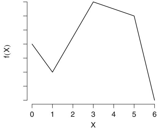
Fig. 2.1 A linear spline function with knots at a = 1, b = 3, c = 5.

2.4.4 Cubic Spline Functions

Although the linear spline is simple and can approximate many common relationships, it is not smooth and will not fit highly curved functions well. These problems can be overcome by using piecewise polynomials of order higher than linear. Cubic polynomials have been found to have nice properties with good ability to fit sharply curving shapes. Cubic splines can be made to be smooth at the join points (knots) by forcing the first and second derivatives of the function to agree at the knots. Such a smooth cubic spline function with three knots (a, b, c) is given by

\[\begin{split} f(X) &= \beta\_0 + \beta\_1 X + \beta\_2 X^2 + \beta\_3 X^3 \\ &+ \beta\_4 (X - a)\_+^3 + \beta\_5 (X - b)\_+^3 + \beta\_6 (X - c)\_+^3 \\ &= X \beta \end{split} \tag{2.22}\]

with the following constructed variables:

\[\begin{aligned} X\_1 &= X \ X\_2 = X^2\\ X\_3 &= X^3 \ X\_4 = (X - a)\_+^3\\ X\_5 &= (X - b)\_+^3 \ X\_6 = (X - c)\_+^3. \end{aligned} \tag{2.23}\]

If the cubic spline function has k knots, the function will require estimating k + 3 regression coefficients besides the intercept. See Section 2.4.6 for information on choosing the number and location of knots. ¹

There are more numerically stable ways to form a design matrix for cubic spline functions that are based on B-splines instead of the truncated power basis152, 575 used here. However, B-splines are more complex and do not allow for extrapolation beyond the outer knots, and the truncated power basis seldom presents estimation problems (see Section 4.6) when modern methods such as the Q–R decomposition are used for matrix inversion. ²

2.4.5 Restricted Cubic Splines

Stone and Koo595 have found that cubic spline functions do have a drawback in that they can be poorly behaved in the tails, that is before the first knot and after the last knot. They cite advantages of constraining the function to be linear in the tails. Their restricted cubic spline function (also called natural ³ splines) has the additional advantage that only k − 1 parameters must be estimated (besides the intercept) as opposed to k + 3 parameters with the unrestricted cubic spline. The restricted spline function with k knots t1,…,t^k is given by156

\[f(X) = \beta\_0 + \beta\_1 X\_1 + \beta\_2 X\_2 + \dots + \beta\_{k-1} X\_{k-1},\tag{2.24}\]

where X¹ = X and for j = 1,…,k − 2,

\[\begin{split} X\_{j+1} &= (X - t\_j)\_+^3 - (X - t\_{k-1})\_+^3 (t\_k - t\_j) / (t\_k - t\_{k-1}) \\ &+ (X - t\_k)\_+^3 (t\_{k-1} - t\_j) / (t\_k - t\_{k-1}). \end{split} \tag{2.25}\]

It can be shown that X^j is linear in X for X ≥ tk. For numerical behavior and to put all basis functions for X on the same scale, R Hmisc and rms package functions by default divide the terms in Eq. 2.25 by

\[ \tau = (t\_k - t\_1)^2. \tag{2.26} \]

Figure 2.2 displays the τ-scaled spline component variables X^j for j = 2, 3, 4 and k = 5 and one set of knots. The left graph magnifies the lower portion of the curves.

require( Hmisc )

x ← rcspline.eval (seq(0,1,.01),
                     knots =seq(.05 ,.95 ,length =5), inclx =T)
xm ← x
xm[xm > .0106 ] ← NA
matplot(x[,1], xm , type ="l", ylim =c(0, .01),
        xlab= expression(X), ylab= ' ' , lty=1)
matplot(x[,1], x, type ="l",
        xlab= expression(X), ylab= ' ' , lty=1)

Figure 2.3 displays some typical shapes of restricted cubic spline functions with k = 3, 4, 5, and 6. These functions were generated using random β.

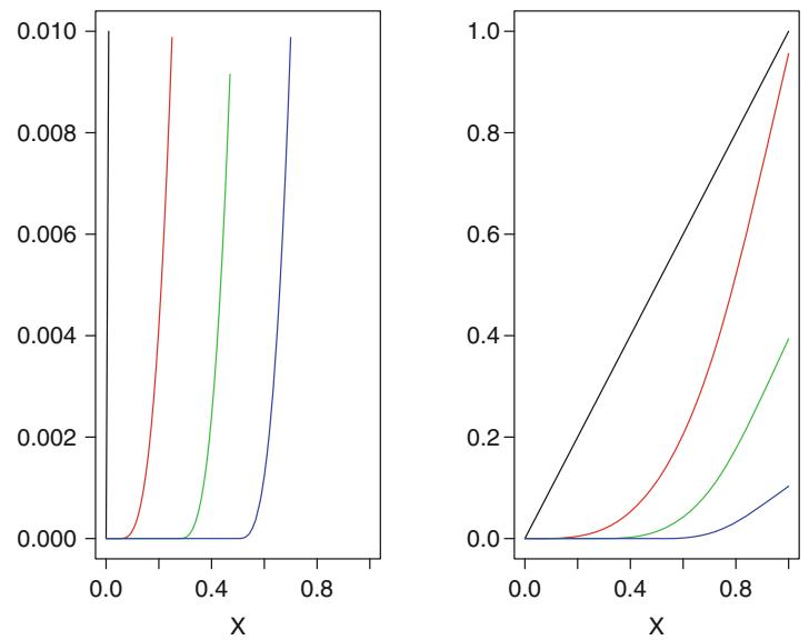
Fig. 2.2 Restricted cubic spline component variables for k = 5 and knots at X = .05, .275, .5, .725, and .95. Nonlinear basis functions are scaled by τ. The left panel is a y–magnification of the right panel. Fitted functions such as those in Figure 2.3 will be linear combinations of these basis functions as long as knots are at the same locations used here.

x ← seq(0, 1, length =300)
for(nk in 3:6) {
  set.seed(nk)
  knots ← seq(.05 , .95 , length =nk)
  xx ← rcspline.eval (x, knots= knots , inclx =T)
  for(i in 1 : (nk - 1))
    xx[,i] ← (xx[,i] - min(xx[,i])) /
               (max(xx[,i]) - min(xx[,i]))
  for(i in 1 : 20) {
    beta ← 2*runif (nk-1) - 1
    xbeta ← xx %*% beta + 2 * runif (1) - 1
    xbeta ← (xbeta - min(xbeta )) /
              (max(xbeta ) - min(xbeta ))
    if(i == 1) {
      plot(x, xbeta , type ="l", lty=1,
            xlab= expression(X), ylab= ' ' , bty="l")
      title (sub=paste (nk ,"knots "), adj=0, cex=.75)
      for(j in 1 : nk)
        arrows (knots [j], .04 , knots [j], -.03 ,
                angle =20, length =.07 , lwd=1.5)
    }
    else lines (x, xbeta , col=i)
  }
}

Once β0,…, βk−¹ are estimated, the restricted cubic spline can be restated in the form

\[\begin{split} f(X) &= \beta\_0 + \beta\_1 X + \beta\_2 (X - t\_1)\_+^3 + \beta\_3 (X - t\_2)\_+^3 \\ &+ \dots + \beta\_{k+1} (X - t\_k)\_+^3 \end{split} \tag{2.27}\]

by dividing β2,…, βk−¹ by τ (Eq. 2.26) and computing

\[\beta\_k = \left[\beta\_2(t\_1 - t\_k) + \beta\_3(t\_2 - t\_k) + \dots + \beta\_{k-1}(t\_{k-2} - t\_k)\right]/(t\_k - t\_{k-1}) \quad \text{(2.28)}\]

\[\beta\_{k+1} = \left[\beta\_2(t\_1 - t\_{k-1}) + \beta\_3(t\_2 - t\_{k-1}) + \dots + \beta\_{k-1}(t\_{k-2} - t\_{k-1})\right]/(t\_{k-1} - t\_k).\]

A test of linearity in X can be obtained by testing

\[H\_0: \beta\_2 = \beta\_3 = \dots = \beta\_{k-1} = 0.\tag{2.29}\]

⁴ The truncated power basis for restricted cubic splines does allow for rational (i.e., linear) extrapolation beyond the outer knots. However, when the outer knots are in the tails of the data, extrapolation can still be dangerous.

When nonlinear terms in Equation 2.25 are normalized, for example, by dividing them by the square of the difference in the outer knots to make all terms have units of X, the ordinary truncated power basis has no numerical difficulties when modern matrix algebra software is used.

2.4.6 Choosing Number and Position of Knots

We have assumed that the locations of the knots are specified in advance; that is, the knot locations are not treated as free parameters to be estimated. If knots were free parameters, the fitted function would have more flexibility but at the cost of instability of estimates, statistical inference problems, and inability to use standard regression modeling software for estimating regression parameters.

How then does the analyst pre-assign knot locations? If the regression relationship were described by prior experience, pre-specification of knot locations would be easy. For example, if a function were known to change curvature at X = a, a knot could be placed at a. However, in most situations there is no way to pre-specify knots. Fortunately, Stone593 has found that the location of knots in a restricted cubic spline model is not very crucial in most situations; the fit depends much more on the choice of k, the number of ⁵ knots. Placing knots at fixed quantiles (percentiles) of a predictor’s marginal distribution is a good approach in most datasets. This ensures that enough points are available in each interval, and also guards against letting outliers overly influence knot placement. Recommended equally spaced quantiles are shown in Table 2.3.

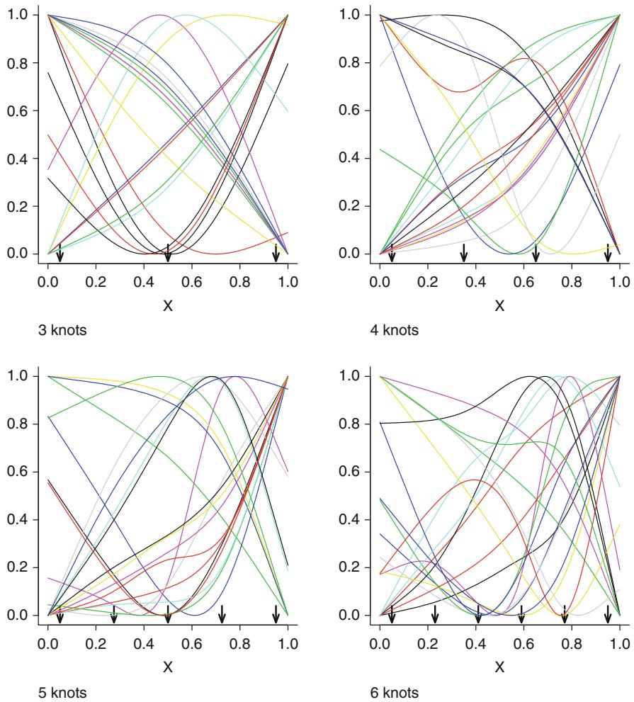
Fig. 2.3 Some typical restricted cubic spline functions for k = 3, 4, 5, 6. The y–axis is Xβ. Arrows indicate knots. These curves were derived by randomly choosing values of β subject to standard deviations of fitted functions being normalized.

Table 2.3 Default quantiles for knots

k	Quantiles
3			.10	.5	.90
4			.05	.35 .65		.95
5		.05	.275	.5	.725	.95
6	.05	.23	.41	.59 .77		.95
7			.025 .1833 .3417 .5			.6583 .8167 .975

The principal reason for using less extreme default quantiles for k = 3 and more extreme ones for k = 7 is that one usually uses k = 3 for small sample sizes and k = 7 for large samples. When the sample size is less than 100, the outer quantiles should be replaced by the fifth smallest and fifth largest data points, respectively.595 What about the choice of k? The flexibility of possible fits must be tempered by the sample size available to estimate the unknown parameters. Stone593 has found that more than 5 knots are seldom required in a restricted cubic spline model. The principal decision then is between k = 3, 4, or 5. For many datasets, k =4offers an adequate fit of the model and is a good compromise between flexibility and loss of precision caused by overfitting a small sample. When the sample size is large (e.g., n ≥ 100 with a continuous uncensored response variable), k = 5 is a good choice. Small samples (< 30, say) may require the use of k = 3. Akaike’s information criterion (AIC, Section 9.8.1) can be used for a data-based choice of k. The value of ^k maximizing the model likelihood ratio ^χ² ⁻ ²^k would be the best “for the money” using AIC.

The analyst may wish to devote more knots to variables that are thought to be more important, and risk lack of fit for less important variables. In this way the total number of estimated parameters can be controlled (Section 4.1).

2.4.7 Nonparametric Regression

One of the most important results of an analysis is the estimation of the tendency (trend) of how X relates to Y . This trend is useful in its own right and it may be sufficient for obtaining predicted values in some situations, but trend estimates can also be used to guide formal regression modeling (by suggesting predictor variable transformations) and to check model assumptions.

Nonparametric smoothers are excellent tools for determining the shape of the relationship between a predictor and the response. The standard nonparametric smoothers work when one is interested in assessing one continuous predictor at a time and when the property of the response that should be linearly related to the predictor is a standard measure of central tendency. For example, when C(Y ) is E(Y ) or Pr[Y = 1], standard smoothers are useful, but when C(Y ) is a measure of variability or a rate (instantaneous risk), or when Y is only incompletely measured for some subjects (e.g., Y is censored for some subjects), simple smoothers will not work.

The oldest and simplest nonparametric smoother is the moving average. Suppose that the data consist of the points X = 1, 2, 3, 5, and 8, with the corresponding Y values 2.1, 3.8, 5.7, 11.1, and 17.2. To smooth the relationship we could estimate E(Y |X = 2) by (2.1+3.8+5.7)/3 and E(Y |X = (2 + 3 + 5)/3) by (3.8+5.7 + 11.1)/3. Note that overlap is fine; that is one point may be contained in two sets that are averaged. You can immediately see that the simple moving average has a problem in estimating E(Y ) at the outer values of X. The estimates are quite sensitive to the choice of the number of points (or interval width) to use in “binning” the data.

A moving least squares linear regression smoother is far superior to a moving flat line smoother (moving average). Cleveland’s111 moving linear regression smoother loess has become the most popular smoother. To obtain the smoothed value of Y at X = x, we take all the data having X values within a suitable interval about x. Then a linear regression is fitted to all of these points, and the predicted value from this regression at X = x is taken as the estimate of E(Y |X = x). Actually, loess uses weighted least squares estimates, which is why it is called a locally weighted least squares method. The weights are chosen so that points near X = x are given the most weightb in the calculation of the slope and intercept. Surprisingly, a good default choice for the interval about x is an interval containing 2/3 of the data points! The weighting function is devised so that points near the extremes of this interval receive almost no weight in the calculation of the slope and intercept.

Because loess uses a moving straight line rather than a moving flat one, it provides much better behavior at the extremes of the Xs. For example, one can fit a straight line to the first three data points and then obtain the predicted value at the lowest X, which takes into account that this X is not the middle of the three Xs.

loess obtains smoothed values for E(Y ) at each observed value of X. Estimates for other Xs are obtained by linear interpolation.

The loess algorithm has another component. After making an initial estimate of the trend line, loess can look for outliers off this trend. It can then delete or down-weight those apparent outliers to obtain a more robust trend estimate. Now, different points will appear to be outliers with respect to this second trend estimate. The new set of outliers is taken into account and another trend line is derived. By default, the process stops after these three iterations. loess works exceptionally well for binary Y as long as the iterations that look for outliers are not done, that is only one iteration is performed.

For a single X, Friedman’s”super smoother”207 is another efficient and flexible nonparametric trend estimator. For both loess and the super smoother the amount of smoothing can be controlled by the analyst. Hastie and Tibshirani275 provided an excellent description of smoothing methods and developed a generalized additive model for multiple Xs, in which each continuous predictor is fitted with a nonparametric smoother (see Chapter 16). Interactions are not allowed. Cleveland et al.96 have extended two- ⁶ dimensional smoothers to multiple dimensions without assuming additivity. Their local regression model is feasible for up to four or so predictors. Local regression models are extremely flexible, allowing parts of the model to be

^b This weight is not to be confused with the regression coefficient; rather the weights are w1, w2,…,wⁿ and the fitting criterion is !ⁿ ⁱ ^wi(Yⁱ ⁻ ^Y^ˆ i)².

parametrically specified, and allowing the analyst to choose the amount of smoothing or the effective number of degrees of freedom of the fit.

Smoothing splines are related to nonparametric smoothers. Here a knot is placed at every data point, but a penalized likelihood is maximized to derive the smoothed estimates. Gray237, 238 developed a general method that is halfway between smoothing splines and regression splines. He pre-specified, say, 10 fixed knots, but uses a penalized likelihood for estimation. This allows 7 the analyst to control the effective number of degrees of freedom used.

Besides using smoothers to estimate regression relationships, smoothers are valuable for examining trends in residual plots. See Sections 14.6 and 21.2 for examples.

2.4.8 Advantages of Regression Splines over Other Methods

There are several advantages of regression splines:271

1. Parametric splines are piecewise polynomials and can be fitted using any existing regression program after the constructed predictors are computed. Spline regression is equally suitable to multiple linear regression, survival models, and logistic models for discrete outcomes.
1. Regression coefficients for the spline function are estimated using standard techniques (maximum likelihood or least squares), and statistical inferences can readily be drawn. Formal tests of no overall association, linearity, and additivity can readily be constructed. Confidence limits for the estimated regression function are derived by standard theory.
1. The fitted spline function directly estimates the transformation that a predictor should receive to yield linearity in C(Y |X). The fitted spline transformation sometimes suggests a simple transformation (e.g., square root) of a predictor that can be used if one is not concerned about the proper number of degrees of freedom for testing association of the predictor with the response.
1. The spline function can be used to represent the predictor in the final model. Nonparametric methods do not yield a prediction equation.
1. Splines can be extended to non-additive models (see below). Multidimensional nonparametric estimators often require burdensome computations.

2.5 Recursive Partitioning: Tree-Based Models

Breiman et al.69 have developed an essentially model-free approach called classification and regression trees (CART), a form of recursive partitioning. For some implementations of CART, we say “essentially” model-free since a model-based statistic is sometimes chosen as a splitting criterion. The essence of recursive partitioning is as follows.

1. Find the predictor so that the best possible binary split on that predictor has a larger value of some statistical criterion than any other split on any other predictor. For ordinal and continuous predictors, the split is of the form X<c versus X ≥ c. For polytomous predictors, the split involves finding the best separation of categories, without preserving order.
1. Within each previously formed subset, find the best predictor and best split that maximizes the criterion in the subset of observations passing the previous split.
1. Proceed in like fashion until fewer than k observations remain to be split, where k is typically 20 to 100.
1. Obtain predicted values using a statistic that summarizes each terminal node (e.g., mean or proportion).
1. Prune the tree backward so that a tree with the same number of nodes developed on 0.9 of the data validates best on the remaining 0.1 of the data (average over the 10 cross-validations). Alternatively, shrink the node estimates toward the mean, using a progressively stronger shrinkage factor, until the best cross-validation results.

Tree models have the advantage of not requiring any functional form for the predictors and of not assuming additivity of predictors (i.e., recursive partitioning can identify complex interactions). Trees can deal with missing data flexibly. They have the disadvantages of not utilizing continuous variables effectively and of overfitting in three directions: searching for best predictors, for best splits, and searching multiple times. The penalty for the extreme amount of data searching required by recursive partitioning surfaces when the tree does not cross-validate optimally until it is pruned all the way back to two or three splits. Thus reliable trees are often not very discriminating. ⁹

Tree models are especially useful in messy situations or settings in which overfitting is not so problematic, such as confounder adjustment using propensity scores117 or in missing value imputation. A major advantage of tree modeling is savings of analyst time, but this is offset by the underfitting needed to make trees validate.

2.6 Multiple Degree of Freedom Tests of Association

When a factor is a linear or binary term in the regression model, the test of association for that factor with the response involves testing only a single regression parameter. Nominal factors and predictors that are represented as a quadratic or spline function require multiple regression parameters to be

tested simultaneously in order to assess association with the response. For a nominal factor having k levels, the overall ANOVA-type test with k − 1 d.f. tests whether there are any differences in responses between the k categories. It is recommended that this test be done before attempting to interpret individual parameter estimates. If the overall test is not significant, it can be dangerous to rely on individual pairwise comparisons because the type I error will be increased. Likewise, for a continuous predictor for which linearity is not assumed, all terms involving the predictor should be tested simultaneously to check whether the factor is associated with the outcome. This test should precede the test for linearity and should usually precede the attempt to eliminate nonlinear terms. For example, in the model

\[C(Y|X) = \beta\_0 + \beta\_1 X\_1 + \beta\_2 X\_2 + \beta\_3 X\_2^2,\tag{2.30}\]

one should test H⁰ : β² = β³ = 0 with 2 d.f. to assess association between X² and outcome. In the five-knot restricted cubic spline model

\[C(Y|X) = \beta\_0 + \beta\_1 X + \beta\_2 X' + \beta\_3 X'' + \beta\_4 X''',\tag{2.31}\]

the hypothesis H⁰ : β¹ = … = β⁴ = 0 should be tested with 4 d.f. to assess whether there is any association between X and Y . If this 4 d.f. test is insignificant, it is dangerous to interpret the shape of the fitted spline function because the hypothesis that the overall function is flat has not been rejected.

A dilemma arises when an overall test of association, say one having 4 d.f., is insignificant, the 3 d.f. test for linearity is insignificant, but the 1 d.f. test for linear association, after deleting nonlinear terms, becomes significant. Had the test for linearity been borderline significant, it would not have been warranted to drop these terms in order to test for a linear association. But with the evidence for nonlinearity not very great, one could attempt to test for association with 1 d.f. This however is not fully justified, because the 1 d.f. test statistic does not have a χ² distribution with 1 d.f. since pretesting was done. The original 4 d.f. test statistic does have a χ² distribution with 4 d.f. because it was for a pre-specified test.

For quadratic regression, Grambsch and O’Brien234 showed that the 2 d.f. test of association is nearly optimal when pretesting is done, even when the true relationship is linear. They considered an ordinary regression model ^E(^Y ^|X) = ^β⁰ ⁺ ^β1^X ⁺ ^β2X² and studied tests of association between ^X and Y . The strategy they studied was as follows. First, fit the quadratic model and obtain the partial test of H⁰ : β² = 0, that is the test of linearity. If this partial F-test is significant at the α = 0.05 level, report as the final test of association between X and Y the 2 d.f. F-test of H⁰ : β¹ = β² = 0. If the test of linearity is insignificant, the model is refitted without the quadratic term and the test of association is then a 1 d.f. test, H⁰ : β¹ = 0|β² = 0. Grambsch and O’Brien demonstrated that the type I error from this twostage test is greater than the stated α, and in fact a fairly accurate P-value can be obtained if it is computed from an F distribution with 2 numerator d.f. even when testing at the second stage. This is because in the original 2 d.f. test of association, the 1 d.f. corresponding to the nonlinear effect is deleted if the nonlinear effect is very small; that is one is retaining the most significant part of the 2 d.f. F statistic.

If we use a 2 d.f. F critical value to assess the X effect even when X² is not in the model, it is clear that the two-stage approach can only lose power and hence it has no advantage whatsoever. That is because the sum of squares due to regression from the quadratic model is greater than the sum of squares computed from the linear model.

2.7 Assessment of Model Fit

2.7.1 Regression Assumptions

In this section, the regression part of the model is isolated, and methods are described for validating the regression assumptions or modifying the model to meet the assumptions. The general linear regression model is

\[C(Y|X) = X\beta = \beta\_0 + \beta\_1 X\_1 + \beta\_2 X\_2 + \dots + \beta\_k X\_k. \tag{2.32}\]

The assumptions of linearity and additivity need to be verified. We begin with a special case of the general model,

\[C(Y|X) = \beta\_0 + \beta\_1 X\_1 + \beta\_2 X\_2,\tag{2.33}\]

where X¹ is binary and X² is continuous. One needs to verify that the property of the response C(Y ) is related to X¹ and X² according to Figure 2.4.

There are several methods for checking the fit of this model. The first method below is based on critiquing the simple model, and the other methods directly “estimate” the model.

Fit the simple linear additive model and critically examine residual plots for evidence of systematic patterns. For least squares fits one can compute estimated residuals ^e ⁼ ^Y ⁻ ^Xβ^ˆ and box plots of ^e stratified by ^X¹ and scatterplots of e versus X¹ and Yˆ with trend curves. If one is assuming constant conditional variance of Y , the spread of the residual distribution against each of the variables can be checked at the same time. If the normality assumption is needed (i.e., if significance tests or confidence limits are used), the distribution of e can be compared with a normal distribution with mean zero. Advantage: Simplicity. Disadvantages: Standard residuals can only be computed for continuous uncensored response variables. The judgment of non-randomness is largely subjective, it is difficult to detect interaction, and if interaction is present it is difficult to check any of the other assumptions. Unless trend lines are added to plots, pat-

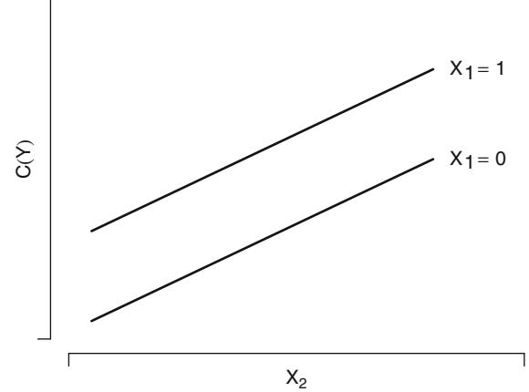
Fig. 2.4 Regression assumptions for one binary and one continuous predictor

terns may be difficult to discern if the sample size is very large. Detecting patterns in residuals does not always inform the analyst of what corrective action to take, although partial residual plots can be used to estimate the needed transformations if interaction is absent.

1. Make a scatterplot of Y versus X² using different symbols according to values of X1. Advantages: Simplicity, and one can sometimes see all regression patterns including interaction. Disadvantages: Scatterplots cannot be drawn for binary, categorical, or censored Y . Patterns are difficult to see if relationships are weak or if the sample size is very large.
1. Stratify the sample by X¹ and quantile groups (e.g., deciles) of X2. Within each X¹ × X² stratum an estimate of C(Y |X1, X2) is computed. If X¹ is continuous, the same method can be used after grouping X¹ into quantile groups. Advantages: Simplicity, ability to see interaction patterns, can handle censored Y if care is taken. Disadvantages: Subgrouping requires relatively large sample sizes and does not use continuous factors effectively as it does not attempt any interpolation. The ordering of quantile groups is not utilized by the procedure. Subgroup estimates have low precision (see p. 488 for an example). Each stratum must contain enough information to allow trends to be apparent above noise in the data. The method of grouping chosen (e.g., deciles vs. quintiles vs. rounding) can alter the shape of the plot.
1. Fit a nonparametric smoother separately for levels of X¹ (Section 2.4.7) relating X² to Y . Advantages: All regression aspects of the model can be summarized efficiently with minimal assumptions. Disadvantages: Does not easily apply to censored Y , and does not easily handle multiple predictors.

Fit a flexible parametric model that allows for most of the departures from the linear additive model that you wish to entertain. Advantages: One framework is used for examining the model assumptions, fitting the model, and drawing formal inference. Degrees of freedom are well defined and all aspects of statistical inference “work as advertised.” Disadvantages: Complexity, and it is generally difficult to allow for interactions when assessing patterns of effects.

The first four methods each have the disadvantage that if confidence limits or formal inferences are desired it is difficult to know how many degrees of freedom were effectively used so that, for example, confidence limits will have the stated coverage probability. For method five, the restricted cubic spline function is an excellent tool for estimating the true relationship between X² and C(Y ) for continuous variables without assuming linearity. By fitting a model containing X² expanded into k − 1 terms, where k is the number of knots, one can obtain an estimate of the function of X² that could be used linearly in the model:

\[\begin{split} \hat{C}(Y|X) &= \hat{\beta}\_0 + \hat{\beta}\_1 X\_1 + \hat{\beta}\_2 X\_2 + \hat{\beta}\_3 X\_2' + \hat{\beta}\_4 X\_2'' \\ &= \hat{\beta}\_0 + \hat{\beta}\_1 X\_1 + \hat{f}(X\_2), \end{split} \tag{2.34}\]

where \[\hat{f}(X\_2) = \hat{\beta}\_2 X\_2 + \hat{\beta}\_3 X\_2' + \hat{\beta}\_4 X\_2'',\tag{2.35}\]

and X′ ² and X′′ ² are constructed spline variables (when k = 4) as described previously. We call ˆf(X2) the spline-estimated transformation of X2. Plotting the estimated spline function ˆf(X2) versus X² will generally shed light on how the effect of X² should be modeled. If the sample is sufficiently large, the spline function can be fitted separately for X¹ = 0 and X¹ = 1, allowing detection of even unusual interaction patterns. A formal test of linearity in X² is obtained by testing H⁰ : β³ = β⁴ = 0, using a computationally efficient score test, for example (Section 9.2.3).

If the model is nonlinear in X2, either a transformation suggested by the spline function plot (e.g., log(X2)) or the spline function itself (by placing X2, X′ ², and X′′ ² simultaneously in any model fitted) may be used to describe X² in the model. If a tentative transformation of X² is specified, say g(X2), the adequacy of this transformation can be tested by expanding g(X2) in a spline function and testing for linearity. If one is concerned only with prediction and not with statistical inference, one can attempt to find a simplifying transformation for a predictor by plotting g(X2) against ˆf(X2) (the estimated spline transformation) for a variety of g, seeking a linearizing transformation of X2. When there are nominal or binary predictors in the model in addition to the continuous predictors, it should be noted that there are no shape assumptions to verify for the binary/nominal predictors. One need only test for interactions between these predictors and the others.

If the model contains more than one continuous predictor, all may be expanded with spline functions in order to test linearity or to describe nonlinear relationships. If one did desire to assess simultaneously, for example, the linearity of predictors X² and X³ in the presence of a linear or binary predictor X1, the model could be specified as

\[\begin{aligned} C(Y|X) &= \beta\_0 + \beta\_1 X\_1 + \beta\_2 X\_2 + \beta\_3 X\_2' + \beta\_4 X\_2'' \\ &+ \beta\_5 X\_3 + \beta\_6 X\_3' + \beta\_7 X\_3'', \end{aligned} \tag{2.36}\]

where X′ 2, X′′ ² , X′ ³, and X′′ ³ represent components of four knot restricted cubic spline functions.

The test of linearity for X² (with 2 d.f.) is H⁰ : β³ = β⁴ = 0. The overall test of linearity for X² and X³ is H⁰ : β³ = β⁴ = β⁶ = β⁷ = 0, with 4 d.f. But as described further in Section 4.1, even though there are many reasons for allowing relationships to be nonlinear, there are reasons for not testing the nonlinear components for significance, as this might tempt the analyst to simplify the model thus distorting inference.234 Testing for linearity is usually best done to justify to non-statisticians the need for complexity to explain or predict outcomes.

2.7.2 Modeling and Testing Complex Interactions

For testing interaction between X¹ and X² (after a needed transformation may have been applied), often a product term (e.g., X1X2) can be added to the model and its coefficient tested. A more general simultaneous test of linearity and lack of interaction for a two-variable model in which one variable is binary (or is assumed linear) is obtained by fitting the model

\[\begin{aligned} C(Y|X) &= \beta\_0 + \beta\_1 X\_1 + \beta\_2 X\_2 + \beta\_3 X\_2' + \beta\_4 X\_2'' \\ &+ \beta\_5 X\_1 X\_2 + \beta\_6 X\_1 X\_2' + \beta\_7 X\_1 X\_2'' \end{aligned} \tag{2.37}\]

and testing H⁰ : β³ = … = β⁷ = 0. This formulation allows the shape of the X² effect to be completely different for each level of X1. There is virtually no departure from linearity and additivity that cannot be detected from this expanded model formulation if the number of knots is adequate and X¹ is binary. For binary logistic models, this method is equivalent to fitting two ¹⁰ separate spline regressions in X2.

Interactions can be complex when all variables are continuous. An approximate approach is to reduce the variables to two transformed variables, in which case interaction may sometimes be approximated by a single product of the two new variables. A disadvantage of this approach is that the estimates of the transformations for the two variables will be different depending

on whether interaction terms are adjusted for when estimating “main effects.” A good compromise method involves fitting interactions of the form X1f(X2) and X2g(X1):

\[\begin{aligned} C(Y|X) &= \beta\_0 + \beta\_1 X\_1 + \beta\_2 X\_1' + \beta\_3 X\_1'' \\ &+ \beta\_4 X\_2 + \beta\_5 X\_2' + \beta\_6 X\_2'' \\ &+ \beta\_7 X\_1 X\_2 + \beta\_8 X\_1 X\_2' + \beta\_9 X\_1 X\_2'' \\ &+ \beta\_{10} X\_2 X\_1' + \beta\_{11} X\_2 X\_1'' \end{aligned} \tag{2.38}\]

(for k = 4 knots for both variables). The test of additivity is H⁰ : β⁷ = β⁸ = … = β¹¹ = 0 with 5 d.f. A test of lack of fit for the simple product interaction with X² is H⁰ : β⁸ = β⁹ = 0, and a test of lack of fit for the simple product interaction with X¹ is H⁰ : β¹⁰ = β¹¹ = 0.

A general way to model and test interactions, although one requiring a larger number of parameters to be estimated, is based on modeling the X¹ × X² × Y relationship with a smooth three-dimensional surface. A cubic spline surface can be constructed by covering the X¹ − X² plane with a grid and fitting a patch-wise cubic polynomial in two variables. The grid is (ui, v^j ), i = 1,…, k, j = 1,…,k, where knots for X¹ are (u1,…,uk) and knots for X² are (v1,…,vk). The number of parameters can be reduced by constraining the surface to be of the form aX¹ + bX² + cX1X² in the lower left and upper right corners of the plane. The resulting restricted cubic spline surface is described by a multiple regression model containing spline expansions in X¹ and X² and all cross-products of the restricted cubic spline components (e.g., X1X′ ²). If the same number of knots k is used for both predictors, the number of interaction terms is (^k ⁻ 1)². Examples of various ways of modeling interaction are given in Chapter 10. Spline functions made up of cross-products of all terms of individual spline functions are called tensor splines. 50, 274 ¹¹

The presence of more than two predictors increases the complexity of tests for interactions because of the number of two-way interactions and because of the possibility of interaction effects of order higher than two. For example, in a model containing age, sex, and diabetes, the important interaction could be that older male diabetics have an exaggerated risk. However, higher-order interactions are often ignored unless specified a priori based on knowledge of the subject matter. Indeed, the number of two-way interactions alone is often too large to allow testing them all with reasonable power while controlling multiple comparison problems. Often, the only two-way interactions we can afford to test are those that were thought to be important before examining the data. A good approach is to test for all such pre-specified interaction effects with a single global (pooled) test. Then, unless interactions involving only one of the predictors are of special interest, one can either drop all interactions or retain all of them.

For some problems a reasonable approach is, for each predictor separately, to test simultaneously the joint importance of all interactions involving that predictor. For p predictors this results in p tests each with p − 1 degrees of freedom. The multiple comparison problem would then be reduced from p(p − 1)/2 tests (if all two-way interactions were tested individually) to p tests.

In the fields of biostatistics and epidemiology, some types of interactions that have consistently been found to be important in predicting outcomes and thus may be pre-specified are the following.

1. Interactions between treatment and the severity of disease being treated. Patients with little disease can receive little benefit.
1. Interactions involving age and risk factors. Older subjects are generally less affected by risk factors. They had to have been robust to survive to their current age with risk factors present.
1. Interactions involving age and type of disease. Some diseases are incurable and have the same prognosis regardless of age. Others are treatable or have less effect on younger patients.
1. Interactions between a measurement and the state of a subject during a measurement. Respiration rate measured during sleep may have greater predictive value and thus have a steeper slope versus outcome than respiration rate measured during activity.
1. Interaction between menopausal status and treatment or risk factors.
1. Interactions between race and disease.
1. Interactions between calendar time and treatment. Some treatments have learning curves causing secular trends in the associations.
1. Interactions between month of the year and other predictors, due to seasonal effects.
1. Interaction between the quality and quantity of a symptom, for example, daily frequency of chest pain × severity of a typical pain episode.
¹² 10. Interactions between study center and treatment.

2.7.3 Fitting Ordinal Predictors

For the case of an ordinal predictor, spline functions are not useful unless there are so many categories that in essence the variable is continuous. When the number of categories k is small (three to five, say), the variable is usually modeled as a polytomous factor using indicator variables or equivalently as one linear term and k − 2 indicators. The latter coding facilitates testing for linearity. For more categories, it may be reasonable to stratify the data by levels of the variable and to compute summary statistics (e.g., logit proportions for a logistic model) or to examine regression coefficients associated with indicator variables over categories. Then one can attempt to summarize the pattern with a linear or some other simple trend. Later hypothesis tests

must take into account this data-driven scoring (by using > 1 d.f., for example), but the scoring can save degrees of freedom when testing for interaction with other factors. In one dataset, the number of comorbid diseases was used to summarize the risk of a set of diseases that was too large to model. By plotting the logit of the proportion of deaths versus the number of diseases, it was clear that the square of the number of diseases would properly score the variables.

Sometimes it is useful to code an ordinal predictor with k − 1 indicator variables of the form [X ≥ v^j ], where j = 2,…,k and [h] is 1 if h is true, 0 otherwise.648 Although a test of linearity does not arise immediately from this coding, the regression coefficients are interpreted as amounts of change from the previous category. A test of whether the last m categories can be combined with the category k − m does follow easily from this coding.

2.7.4 Distributional Assumptions

The general linear regression model is stated as C(Y |X) = Xβ to highlight its regression assumptions. For logistic regression models for binary or nominal responses, there is no distributional assumption if simple random sampling is used and subjects’ responses are independent. That is, the binary logistic model and all of its assumptions are contained in the expression logit{Y = ¹|X} ⁼ ^Xβ. For ordinary multiple regression with constant variance ^σ², we usually assume that Y −Xβ is normally distributed with mean 0 and variance σ². This assumption can be checked by estimating β with βˆ and plotting the overall distribution of the residuals ^Y ⁻ ^Xβˆ, the residuals against ^Y^ˆ , and the residuals against each X. For the latter two, the residuals should be normally distributed within each neighborhood of Yˆ or X. A weaker requirement is that the overall distribution of residuals is normal; this will be satisfied if all of the stratified residual distributions are normal. Note a hidden assumption in both models, namely, that there are no omitted predictors. Other models, such as the Weibull survival model or the Cox132 proportional hazards model, also have distributional assumptions that are not fully specified by C(Y |X) = Xβ. However, regression and distributional assumptions of some of these models are encapsulated by

\[C(Y|X) = C(Y = y|X) = d(y) + X\beta \tag{2.39}\]

for some choice of C. Here C(Y = y|X) is a property of the response Y evaluated at Y = y, given the predictor values X, and d(y) is a component of the distribution of Y . For the Cox proportional hazards model, C(Y = y|X) can be written as the log of the hazard of the event at time y, or equivalently as the log of the − log of the survival probability at time y, and d(y) can be thought of as a log hazard function for a “standard” subject.

If we evaluated the property ^C(^Y ⁼ ^y|X) at predictor values ^X¹ and ^X2, the difference in properties is

\[\begin{aligned} C(Y=y|X^1) - C(Y=y|X^2) &= d(y) + X^1 \beta \\ &- [d(y) + X^2 \beta] \\ &= (X^1 - X^2)\beta, \end{aligned} \tag{2.40}\]

which is independent of y. One way to verify part of the distributional assumption is to estimate ^C(^Y ⁼ ^y|X1) and ^C(^Y ⁼ ^y|X2) for set values of X¹ and X² using a method that does not make the assumption, and to plot ^C(^Y ⁼ ^y|X1) ⁻ ^C(^Y ⁼ ^y|X2) versus ^y. This function should be flat if the distributional assumption holds. The assumption can be tested formally if d(y) can be generalized to be a function of X as well as y. A test of whether d(y|X) depends on X is a test of one part of the distributional assumption. For example, writing d(y|X) = d(y) + XΓ log(y) where

\[X\varGamma = \varGamma\_1 X\_1 + \varGamma\_2 X\_2 + \dots + \varGamma\_k X\_k \tag{2.41}\]

and testing H⁰ : Γ¹ = … = Γ^k = 0 is one way to test whether d(y|X) depends on X. For semiparametric models such as the Cox proportional hazards model, the only distributional assumption is the one stated above, namely, that the difference in properties between two subjects depends only on the difference in the predictors between the two subjects. Other, parametric, models assume in addition that the property C(Y = y|X) has a specific shape as a function of y, that is that d(y) has a specific functional form. For example, the Weibull survival model has a specific assumption regarding the shape of the hazard or survival distribution as a function of y.

Assessments of distributional assumptions are best understood by applying these methods to individual models as is demonstrated in later chapters.

2.8 Further Reading

1 References [152, 575, 578] have more information about cubic splines.
2 See Smith578 for a good overview of spline functions.
3 More material about natural splines may be found in de Boor152. McNeil et al.451 discuss the overall smoothness of natural splines in terms of the integral of the square of the second derivative of the regression function, over the range of the data. Govindarajulu et al.230 compared restricted cubic splines, penalized splines, and fractional polynomial532 fits and found that the first two methods agreed with each other more than with estimated fractional polynomials.
4 A tutorial on restricted cubic splines is in [271].
5 Durrleman and Simon168 provide examples in which knots are allowed to be estimated as free parameters, jointly with the regression coefficients. They found that even though the “optimal” knots were often far from a priori knot locations, the model fits were virtually identical.

2.8 Further Reading 41

6 Contrast Hastie and Tibshirani’s generalized nonparametric additive models275 with Stone and Koo’s595 additive model in which each continuous predictor is represented with a restricted cubic spline function.
7 Gray237,238 provided some comparisons with ordinary regression splines, but he compared penalized regression splines with non-restricted splines with only two knots. Two knots were chosen so as to limit the degrees of freedom needed by the regression spline method to a reasonable number. Gray argued that regression splines are sensitive to knot locations, and he is correct when only two knots are allowed and no linear tail restrictions are imposed. Two knots also prevent the (ordinary maximum likelihood) fit from utilizing some local behavior of the regression relationship. For penalized likelihood estimation using B-splines, Gray238 provided extensive simulation studies of type I and II error for testing association in which the true regression function, number of knots, and amount of likelihood penalization were varied. He studied both normal regression and Cox regression.
8 Breiman et al.’s original CART method69 used the Gini criterion for splitting. Later work has used log-likelihoods.109 Segal,562 LeBlanc and Crowley,389 and Ciampi et al.107,108 and Kele¸s and Segal342have extended recursive partitioning to censored survival data using the log-rank statistic as the criterion. Zhang682 extended tree models to handle multivariate binary responses. Schmoor et al.556 used a more general splitting criterion that is useful in therapeutic trials, namely, a Cox test for main and interacting effects. Davis and Anderson149 used an exponential survival model as the basis for tree construction. Ahn and Loh7 developed a Cox proportional hazards model adaptation of recursive partitioning along with bootstrap and cross-validation-based methods to protect against “over-splitting.” The Cox-based regression tree methods of Ciampi et al.107 have a unique feature that allows for construction of “treatment interaction trees” with hierarchical adjustment for baseline variables. Zhang et al.683 provided a new method for handling missing predictor values that is simpler than using surrogate splits. See [34,140,270,629] for examples using recursive partitioning for binary responses in which the prediction trees did not validate well. 9 443,629 discuss other problems with tree models.
10 For ordinary linear models, the regression estimates are the same as obtained with separate fits, but standard errors are different (since a pooled standard error is used for the combined fit). For Cox132 regression, separate fits can be slightly different since each subset would use a separate ranking of Y .
11 Gray’s penalized fixed-knot regression splines can be useful for estimating joint effects of two continuous variables while allowing the analyst to control the effective number of degrees of freedom in the fit [237, 238, Section 3.2]. When Y is a non-censored variable, the local regression model of Cleveland et al.,96 a multidimensional scatterplot smoother mentioned in Section 2.4.7, provides a good graphical assessment of the joint effects of several predictors so that the forms of interactions can be chosen. See Wang et al.653 and Gustafson248 for several other flexible approaches to analyzing interactions among continuous variables.
12 Study site by treatment interaction is often the interaction that is worried about the most in multi-center randomized clinical trials, because regulatory agencies are concerned with consistency of treatment effects over study centers. However, this type of interaction is usually the weakest and is difficult to assess when there are many centers due to the number of interaction parameters to estimate. Schemper545 discusses various types of interactions and a general nonparametric test for interaction.

2.9 Problems

For problems 1 to 3, state each model statistically, identifying each predictor with one or more component variables. Identify and interpret each regression parameter except for coefficients of nonlinear terms in spline functions. State each hypothesis below as a formal statistical hypothesis involving the proper parameters, and give the (numerator) degrees of freedom of the test. State alternative hypotheses carefully with respect to unions or intersections of conditions and list the type of alternatives to the null hypothesis that the test is designed to detect.c

1. A property of Y such as the mean is linear in age and blood pressure and there may be an interaction between the two predictors. Test H⁰ : there is no interaction between age and blood pressure. Also test H⁰ : blood pressure is not associated with Y (in any fashion). State the effect of blood pressure as a function of age, and the effect of age as a function of blood pressure.
1. Consider a linear additive model involving three treatments (control, drug Z, and drug Q) and one continuous adjustment variable, age. Test H⁰ : treatment group is not associated with response, adjusted for age. Also test H⁰ : response for drug Z has the same property as the response for drug Q, adjusted for age.
1. Consider models each with two predictors, temperature and white blood count (WBC), for which temperature is always assumed to be linearly related to the appropriate property of the response, and WBC may or may not be linear (depending on the particular model you formulate for each question). Test:
- 1. H⁰ : WBC is not associated with the response versus H^a : WBC is linearly associated with the property of the response.
- 1. H⁰ : WBC is not associated with Y versus H^a : WBC is quadratically associated with Y . Also write down the formal test of linearity against this quadratic alternative.
- 1. H⁰ : WBC is not associated with Y versus H^a : WBC related to the property of the response through a smooth spline function; for example, for WBC the model requires the variables WBC, WBC′ , and WBC′′ where WBC′ and WBC′′ represent nonlinear components (if there are four knots in a restricted cubic spline function). Also write down the formal test of linearity against this spline function alternative.
- 1. Test for a lack of fit (combined nonlinearity or non-additivity) in an overall model that takes the form of an interaction between temperature and WBC, allowing WBC to be modeled with a smooth spline function.
1. For a fitted model Y = a + bX + cX² derive the estimate of the effect on Y of changing X from x¹ to x2.

^c In other words, under what assumptions does the test have maximum power?

2.9 Problems 43

1. In “The Class of 1988: A Statistical Portrait,” the College Board reported mean SAT scores for each state. Use an ordinary least squares multiple regression model to study the mean verbal SAT score as a function of the percentage of students taking the test in each state. Provide plots of fitted functions and defend your choice of the “best” fit. Make sure the shape of the chosen fit agrees with what you know about the variables. Add the raw data points to plots.
- 1. Fit a linear spline function with a knot at X = 50%. Plot the data and the fitted function and do a formal test for linearity and a test for association between X and Y . Give a detailed interpretation of the estimated coefficients in the linear spline model, and use the partial t-test to test linearity in this model.
- 1. Fit a restricted cubic spline function with knots at X = 6, 12, 58, and 68% (not percentile).d Plot the fitted function and do a formal test of association between X and Y . Do two tests of linearity that test the same hypothesis:
  - 1. by using a contrast to simultaneously test the correct set of coefficients against zero (done by the anova function in rms);e
  - 1. by comparing the R² from the complex model with that from a simple linear model using a partial F-test.

Explain why the tests of linearity have the d.f. they have.

Using subject matter knowledge, pick a final model (from among the previous models or using another one) that makes sense.

The data are found in Table 2.4 and may be created in R using the sat.r code on the RMS course web site.

1. Derive the formulas for the restricted cubic spline component variables without cubing or squaring any terms.
1. Prove that each component variable is linear in X when X ≥ tk, the last knot, using general principles and not algebra or calculus. Derive an expression for the restricted spline regression function when X ≥ tk.
1. Consider a two–stage procedure in which one tests for linearity of the effect of a predictor X on a property of the response C(Y |X) against a quadratic alternative. If the two–tailed test of linearity is significant at the α level, a two d.f. test of association between X and Y is done. If the test for linearity is not significant, the square term is dropped and a linear model is fitted. The test of association between X and Y is then (apparently) a one d.f. test.
- 1. Write a formal expression for the test statistic for association.

^d Note: To pre-specify knots for restricted cubic spline functions, use something like rcs(predictor, c(t1,t2,t3,t4)), where the knot locations are t1, t2, t3, t4.

^e Note that anova in rms computes all needed test statistics from a single model fit object.

1. Write an expression for the nominal P–value for testing association using this strategy.
1. Write an expression for the actual P–value or alternatively for the type– I error if using a fixed critical value for the test of association.
1. For the same two–stage strategy consider an estimate of the effect on C(Y |X) of increasing X from a to b. Write a brief symbolic algorithm for deriving a true two–sided 1−α confidence interval for the b : a effect (difference in C(Y )) using the bootstrap.

	% Taking SAT Mean Verbal % Taking SAT Mean Verbal
(X)	Score (Y )	(X)	Score (Y )
4	482	24	440
5	498	29	460
5	513	37	448
6	498	43	441
6	511	44	424
7	479	45	417
9	480	49	422
9	483	50	441
10	475	52	408
10	476	55	412
10	487	57	400
10	494	58	401
12	474	59	430
12	478	60	433
13	457	62	433
13	485	63	404
14	451	63	424
14	471	63	430
14	473	64	431
16	467	64	437
17	470	68	446
18	464	69	424
20	471	72	420
22	455	73	432
23	452	81	436

Table 2.4 SAT data from the College Board, 1988

Chapter 3 Missing Data

3.1 Types of Missing Data

There are missing data in the majority of datasets one is likely to encounter. Before discussing some of the problems of analyzing data in which some variables are missing for some subjects, we define some nomenclature. ¹

Missing completely at random (MCAR)

Data are missing for reasons that are unrelated to any characteristics or responses for the subject, including the value of the missing value, were it to be known. Examples include missing laboratory measurements because of a dropped test tube (if it was not dropped because of knowledge of any measurements), a study that ran out of funds before some subjects could return for follow-up visits, and a survey in which a subject omitted her response to a question for reasons unrelated to the response she would have made or to any other of her characteristics.

Missing at random (MAR)

Data are not missing at random, but the probability that a value is missing depends on values of variables that were actually measured. As an example, consider a survey in which females are less likely to provide their personal income in general (but the likelihood of responding is independent of her actual income). If we know the sex of every subject and have income levels for some of the females, unbiased sex-specific income estimates can be made. That is because the incomes we do have for some of the females are a random sample of all females’ incomes. Another way of saying that a variable is MAR

is that given the values of other available variables, subjects having missing values are only randomly different from other subjects.535 Or to paraphrase Greenland and Finkle,242 for MAR the missingness of a covariable cannot depend on unobserved covariable values; for example whether a predictor is observed cannot depend on another predictor when the latter is missing but it can depend on the latter when it is observed. MAR and MCAR data are also called ignorable non-responses.

Informative missing (IM)

The tendency for a variable to be missing is a function of data that are not available, including the case when data tend to be missing if their true values are systematically higher or lower. An example is when subjects with lower income levels or very high incomes are less likely to provide their personal income in an interview. IM is also called nonignorable non-response and missing not at random (MNAR).

IM is the most difficult type of missing data to handle. In many cases, there is no fix for IM nor is there a way to use the data to test for the existence of IM. External considerations must dictate the choice of missing data models, and there are few clues for specifying a model under IM. MCAR is the easiest case to handle. Our ability to correctly analyze MAR data depends on the availability of other variables (the sex of the subject in the example above). Most of the methods available for dealing with missing data assume the data are MAR. Fortunately, even though the MAR assumption is not testable, it may hold approximately if enough variables are included in the imputation models256.

3.2 Prelude to Modeling

No matter whether one deletes incomplete cases, carefully imputes (estimates) missing data, or uses a full maximum likelihood or Bayesian techniques to incorporate partial data, it is beneficial to characterize patterns of missingness using exploratory data analysis techniques. These techniques include binary logistic models and recursive partitioning for predicting the probability that a given variable is missing. Patterns of missingness should be reported to help readers understand the limitations of incomplete data. If you do decide to use imputation, it is also important to describe how variables are simultaneously missing. A cluster analysis of missing value status of all the variables is useful here. This can uncover cases where imputation is not as effective. For example, if the only variable moderately related to diastolic blood pressure is systolic pressure, but both pressures are missing on the same subjects, systolic pressure cannot be used to estimate diastolic blood pressure. R functions naclus and naplot in the Hmisc package (see p. 142) can help detect how variables are simultaneously missing. Recursive partitioning (regression tree) algorithms (see Section 2.5) are invaluable for describing which kinds of subjects are missing on a variable. Logistic regression is also an excellent tool for this purpose. A later example (p. 302) demonstrates these procedures.

It can also be helpful to explore the distribution of non-missing Y by the number of missing variables in X (including zero, i.e., complete cases on X).

3.3 Missing Values for Different Types of Response Variables

When the response variable Y is collected serially but some subjects drop out of the study before completion, there are many ways of dealing with partial information42, 412, 480 including multiple imputation in phases,381 or efficiently analyzing all available serial data using a full likelihood model. When Y is the time until an event, there are actually no missing values of Y but follow-up will be curtailed for some subjects. That leaves the case where the response is completely measured once.

It is common practice to discard subjects having missing Y . Before doing so, at minimum an analysis should be done to characterize the tendency for Y to be missing, as just described. For example, logistic regression or recursive partitioning can be used to predict whether Y is missing and to test for systematic tendencies as opposed to Y being missing completely at random. In many models, though, more efficient and less biased estimates of regression coefficients can be made by also utilizing observations missing on Y that are non-missing on X. Hence there is a definite place for imputation of Y . von Hippel645 found advantages of using all variables to impute all others, and once imputation is finished, discarding those observations having missing Y . However if missing Y values are MCAR, up-front deletion of cases having missing Y may sometimes be preferred, as imputation requires correct specification of the imputation model. ²

3.4 Problems with Simple Alternatives to Imputation

Incomplete predictor information is a very common missing data problem. Statistical software packages use casewise deletion in handling missing predictors; that is, any subject having any predictor or Y missing will be excluded from a regression analysis. Casewise deletion results in regression coefficient estimates that can be terribly biased, imprecise, or both353. First consider an example where bias is the problem. Suppose that the response is death and

the predictors are age, sex, and blood pressure, and that age and sex were recorded for every subject. Suppose that blood pressure was not measured for a fraction of 0.10 of the subjects, and the most common reason for not obtaining a blood pressure was that the subject was about to die. Deletion of these very sick patients will cause a major bias (downward) in the model’s 3 intercept parameter. In general, casewise deletion will bias the estimate of the model’s intercept parameter (as well as others) when the probability of a case being incomplete is related to Y and not just to X [422, Example 3.3]. van der Heijden et al.628 discuss how complete case analysis (casewise deletion) usually assumes MCAR.

Now consider an example in which casewise deletion of incomplete records is inefficient. The inefficiency comes from the reduction of sample size, which causes standard errors to increase,162 confidence intervals to widen, and power of tests of association and tests of lack of fit to decrease. Suppose that the response is the presence of coronary artery disease and the predictors are age, sex, LDL cholesterol, HDL cholesterol, blood pressure, triglyceride, and smoking status. Suppose that age, sex, and smoking are recorded for all subjects, but that LDL is missing in 0.18 of the subjects, HDL is missing in 0.20, and triglyceride is missing in 0.21. Assume that all missing data are MCAR and that all of the subjects missing LDL are also missing HDL and that overall 0.28 of the subjects have one or more predictors missing and hence would be excluded from the analysis. If total cholesterol were known on every subject, even though it does not appear in the model, it (along perhaps with age and sex) can be used to estimate (impute) LDL and HDL cholesterol and triglyceride, perhaps using regression equations from other studies. Doing the analysis on a “filled in” dataset will result in more precise estimates because the sample size would then include the other 0.28 of the subjects.

In general, observations should only be discarded if the MCAR assumption is justified, there is a rarely missing predictor of overriding importance that cannot be reliably imputed from other information, or if the fraction of observations excluded is very small and the original sample size is large. Even then, there is no advantage of such deletion other than saving analyst time. If a predictor is MAR but its missingness depends on Y , casewise deletion is biased.

The first blood pressure example points out why it can be dangerous to handle missing values by adding a dummy variable to the model. Many analysts would set missing blood pressures to a constant (it doesn’t matter which constant) and add a variable to the model such as is.na(blood.pressure) in R notation. The coefficient for the latter dummy variable will be quite large in the earlier example, and the model will appear to have great ability to predict death. This is because some of the left-hand side of the model contaminates the right-hand side; that is, is.na(blood.pressure) is correlated ⁴ with death. For categorical variables, another common practice is to add a new category to denote missing, adding one more degree of freedom to the predictor and changing its meaning.a Jones326, Allison [12, pp. 9–11], Donders et al.161, Knol et al.353 and van der Heijden et al.628 describe why both of these missing-indicator methods are invalid even when MCAR holds. 5

3.5 Strategies for Developing an Imputation Model

Except in special circumstances that usually involve only very simple models, the primary alternative to deleting incomplete observations is imputation of the missing values. Many non-statisticians find the notion of estimating data distasteful, but the way to think about imputation of missing values is that “making up” data is better than discarding valuable data. It is especially distressing to have to delete subjects who are missing on an adjustment variable when a major variable of interest is not missing. So one goal of imputation is to use as much information as possible for examining any one predictor’s adjusted association with Y . The overall goal of imputation is to preserve the information and meaning of the non-missing data.

At this point the analyst must make some decisions about the information to use in computing predicted values for missing values.

1. Imputation of missing values for one of the variables can ignore all other information. Missing values can be filled in by sampling non-missing values of the variable, or by using a constant such as the median or mean nonmissing value.
1. Imputation algorithms can be based only on external information not otherwise used in the model for Y in addition to variables included in later modeling. For example, family income can be imputed on the basis of location of residence when such information is to remain confidential for other aspects of the analysis or when such information would require too many degrees of freedom to be spent in the ultimate response model.
1. Imputations can be derived by only analyzing interrelationships among the Xs.
1. Imputations can use relationships among the Xs and between X and Y .
1. Imputations can use X, Y , and auxiliary variables not in the model predicting Y .
1. Imputations can take into account the reason for non-response if known.

The model to estimate the missing values in a sometimes-missing (target) variable should include all variables that are either

^a This may work if values are “missing” because of “not applicable”, e.g. one has a measure of marital happiness, dichotomized as high or low, but the sample contains some unmarried people. One could have a 3-category variable with values high, low, and unmarried (Paul Allison, IMPUTE e-mail list, 4Jul09).

1. related to the missing data mechanism;
1. have distributions that differ between subjects that have the target variable missing and those that have it measured;
1. are associated with the target variable when it is not missing; or
1. are included in the final response model43.

The imputation and analysis (response) models should be “congenial” or the imputation model should be more general than the response model or make well-founded assumptions256.

When a variable, say X^j , is to be included as a predictor of Y , and X^j is sometimes missing, ignoring the relationship between X^j and Y for those observations for which both are known will bias regression coefficients for X^j toward zero in the outcome model.421 On the other hand, using Y to singly impute X^j using a conditional mean will cause a large inflation in the apparent importance of X^j in the final model. In other words, when the missing X^j are replaced with a mean that is conditional on Y without a random component, this will result in a falsely strong relationship between the imputed X^j values and Y .

At first glance it might seem that using Y to impute one or more of the Xs, even with allowance for the correct amount of random variation, would result in a circular analysis in which the importance of the Xs will be exaggerated. But the relationship between X and Y in the subset of imputed observations will only be as strong as the associations between X and Y that are evidenced by the non-missing data. In other words, regression coefficients estimated from a dataset that is completed by imputation will not in general be biased high as long as the imputed values have similar variation as non-missing data values.

The next important decision about developing imputation algorithms is the choice of how missing values are estimated.

1. Missings can be estimated using single “best guesses” (e.g., predicted conditional expected values or means) based on relationships between nonmissing values. This is called single imputation of conditional means.
1. Missing X^j (or Y ) can be estimated using single individual predicted values, where by predicted value we mean a random variable value from the whole conditional distribution of Xj. If one uses ordinary multiple regression to estimate X^j from Y and the other Xs, a random residual would be added to the predicted mean value. If assuming a normal distribution for X^j conditional on the other data, such a residual could be computed by a Gaussian random number generator given an estimate of the residual standard deviation. If normality is not assumed, the residual could be a randomly chosen residual from the actual computed residuals. When m missing values need imputation for Xj, the residuals could be sampled with replacement from the entire vector of residuals as in the bootstrap. Better still according to Rubin and Schenker535 would be to use the “approximate Bayesian bootstrap” which involves sampling n residuals with

replacement from the original n estimated residuals (from observations not missing on X^j ), then sampling m residuals with replacement from the first sampled set. 6

1. More than one random predicted value (as just defined) can be generated for each missing value. This process is called multiple imputation and it has many advantages over the other methods in general. This is discussed in Section 3.8.
1. Matching methods can be used to obtain random draws of other subject’s values to replace missing values. Nearest neighbor matching can be used to select a subject that is “close” to the subject in need of imputation, on the basis of a series of variables. This method requires the analyst to make decisions about what constitutes “closeness.” To simplify the matching process into a single dimension, Little420 proposed the predictive mean matching method where matching is done on the basis of predicted values from a regression model for predicting the sometimes-missing variable (section 3.7). According to Little, in large samples predictive mean matching may be more robust to model misspecification than the method of adding a random residual to the subject’s predicted value, but because of difficulties in finding matches the random residual method may be better in smaller samples. The random residual method may be easier to use when multiple imputations are needed, but care must be taken to create the correct degree of uncertainty in residuals. ⁷

What if X^j needs to be imputed for some subjects based on other variables that themselves may be missing on the same subjects missing on X^j ? This is a place where recursive partitioning with “surrogate splits” in case of missing predictors may be a good method for developing imputations (see Section 2.5 and p. 142). If using regression to estimate missing values, an algorithm to cycle through all sometimes-missing variables for multiple iterations may perform well. This algorithm is used by the R transcan function described in Section 4.7.4 as well as the to–be–described aregImpute function. First, all missing values are initialized to medians (modes for categorical variables). Then every time missing values are estimated for a certain variable, those estimates are inserted the next time the variable is used to predict other sometimes-missing variables.

If you want to assess the importance of a specific predictor that is frequently missing, it is a good idea to perform a sensitivity analysis in which all observations containing imputed values for that predictor are temporarily deleted. The test based on a model that included the imputed values may be diluted by the imputation or it may test the wrong hypothesis, especially if Y is not used in imputing X.

Little argues for down-weighting observations containing imputations, to obtain a more accurate variance–covariance matrix. For the ordinary linear model, the weights have been worked out for some cases [421, p. 1231].

3.6 Single Conditional Mean Imputation

For a continuous or binary X that is unrelated to all other predictor variables, the mean or median may be substituted for missing values without much loss of efficiency,162 although regression coefficients will be biased low since Y was not utilized in the imputation. When the variable of interest is related to the other Xs, it is far more efficient to use an individual predictive model for each X based on the other variables.79, 525, 612 The “best guess” imputation method fills in missings with predicted expected values using the multivariable imputation model based on non-missing datab. It is true that conditional means are the best estimates of unknown values, but except perhaps for binary logistic regression621, 623 their use will result in biased estimates and very biased (low) variance estimates. The latter problem arises from the reduced variability of imputed values [174, p. 464].

Tree-based models (Section 2.5) may be very useful for imputation since they do not require linearity or additivity assumptions, although such models often have poor discrimination when they don’t overfit. When a continuous X being imputed needs to be non-monotonically transformed to best relate it to the other Xs (e.g., blood pressure vs. heart rate), trees and ordinary regression are inadequate. Here a general transformation modeling procedure (Section 4.7) may be needed.

Schemper et al.551, 553 proposed imputing missing binary covariables by predicted probabilities. For categorical sometimes-missing variables, imputation models can be derived using polytomous logistic regression or a classification tree method. For missing values, the most likely value for each subject (from the series of predicted probabilities from the logistic or recursive partitioning model) can be substituted to avoid creating a new category that is falsely highly correlated with Y . For an ordinal X, the predicted mean value (possibly rounded to the nearest actual data value) or median value from an ⁸ ordinal logistic model is sometimes useful.

3.7 Predictive Mean Matching

In predictive mean matching422 (PMM), one replaces a missing (NA) value for the target variable being imputed with the actual value from a donor observation. Donors are identified by matching in only one dimension, namely the predicted value (e.g., predicted mean) of the target. Key considerations are how to

^b Predictors of the target variable include all the other Xs along with auxiliary variables that are not included in the final outcome model, as long as they precede the variable being imputed in the causal chain (unlike with multiple imputation).

1. model the target when it is not NA
1. match donors on predicted values
1. avoid overuse of “good” donors to disallow excessive ties in imputed data
1. account for all uncertainties (section 3.8).

The predictive model for each target variable uses any outcome variables, all predictors in the final outcome model, plus any needed auxiliary variables. The modeling method should be flexible, not assuming linearity. Many methods will suffice; parametric additive models are often good choices. Beauties of PMM include the lack of need for distributional assumptions (as no residuals are calculated), and predicted values need only be monotonically related to real predicted valuesc

In the original PMM method the donor for an NA was the complete observation whose predicted target was closest to the predicted value of the target from all complete observationsd. This approach can result in some donors being used repeatedly. This can be addressed by sampling from a multinomial distribution, where the probabilities are scaled distances of all potential donors’ predictions to the predicted value y^∗ of the missing target. Tukey’s tricube function (used in loess) is a good weighting function, implemented in the Hmisc aregImpute function:

\[\begin{aligned} w\_i &= (1 - \min(d\_i/s, 1)^3)^3, \\ d\_i &= |\hat{y}\_i - y^\*| \\ s &= 0.2 \times \text{mean} |\hat{y}\_i - y^\*|. \end{aligned} \tag{3.1}\]

s above is a good default scale factor, and the wⁱ are scaled so that !wⁱ = 1.

3.8 Multiple Imputation

Imputing missing values and then doing an ordinary analysis as if the imputed values were real measurements is usually better than excluding subjects with incomplete data. However, ordinary formulas for standard errors and other statistics are invalid unless imputation is taken into account.651 Methods for properly accounting for having incomplete data can be complex. The bootstrap (described later) is an easy method to implement, but the computations can be slowe.

^c Thus when modeling binary or categorical targets one can frequently take least squares shortcuts in place of maximum likelihood for binary, ordinal, or multinomial logistic models.

^d 662 discusses an alternative method based on choosing a donor observation at random from the q closest matches (q = 3, for example).

^e To use the bootstrap to correctly estimate variances of regression coefficients, one must repeat the imputation process and the model fitting perhaps 100 times using a

Multiple imputation uses random draws from the conditional distribution of the target variable given the other variables (and any additional information that is relevant)85, 417, 421, 536 ⁹ . The additional information used to predict the missing values can contain any variables that are potentially predictive, including variables measured in the future; the causal chain is not relevant.421, 463 When a regression model is used for imputation, the process involves adding a random residual to the “best guess” for missing values, to yield the same conditional variance as the original variable. Methods for estimating residuals were listed in Section 3.5. To properly account for variability due to unknown values, the imputation is repeated M times, where M ≥ 3. Each repetition results in a “completed” dataset that is analyzed using the standard method. Parameter estimates are averaged over these multiple imputations to obtain better estimates than those from single imputation. The variance–covariance matrix of the averaged parameter estimates, adjusted for variability due to imputation, is estimated using422

\[V = M^{-1} \sum\_{i}^{M} V\_i + \frac{M+1}{M} B,\tag{3.2}\]

where Vⁱ is the ordinary complete data estimate of the variance–covariance matrix for the model parameters from the ith imputation, and B is the between-imputation sample variance–covariance matrix, the diagonal entries ¹⁰ of which are the ordinary sample variances of the M parameter estimates.

After running aregImpute (or MICE) you can run the Hmisc packages’s fit.mult.impute function to fit the chosen model separately for each artificially completed dataset corresponding to each imputation. After fit.mult.impute fits all of the models, it averages the sets of regression coefficients and computes variance and covariance estimates that are adjusted for imputation (using Eq. 3.2).

White and Royston661 provide a method for multiply imputing missing covariate values using censored survival time data in the context of the Cox proportional hazards model.

White et al.662 recommend choosing the number of imputations M so that the key inferential statistics are very reproducible should the imputation analysis be repeated. They suggest the use of 100f imputations when f is the fraction of cases that are incomplete. See also [85, Section 2.7] and232. Extreme amount of missing data does not prevent one from using multiple imputation, because alternatives are worse321. Horton and Lipsitz302 also have a good overview of multiple imputation and a review of several software packages that implement PMM.

Caution: Multiple imputation methods can generate imputations having very reasonable distributions but still not having the property that final

resampling procedure174,566 (see Section 5.2). Still, the bootstrap can estimate the right variance for the wrong parameter estimates if the imputations are not done correctly.

response model regression coefficients have nominal confidence interval coverage. Among other things, it is worth checking that imputations generate the correct collinearities among covariates.

3.8.1 The aregImpute and Other Chained Equations Approaches

A flexible approach to multiple imputation that handles a wide variety of target variables to be imputed and allows for multiple variables to be missing on the same subject is the chained equation method. With a chained equations approach, each target variable is predicted by a regression model conditional on all other variables in the model, plus other variables. An iterative process cycles through all target variables to impute all missing values627. This approach is used in the MICE algorithm (multiple imputation using chained equations) implemented in R and other systems. The chained equation method does not attempt to use the full Bayesian multivariate model for all target variables, which makes it more flexible and easy to use but leaves it open to creating improper imputations, e.g., imputing conflicting values for different target variables. However, simulation studies627 so far have demonstrated very good performance of imputation based on chained equations in non-complex situations.

The aregImpute algorithm463 takes all aspects of uncertainty into account using the bootstrap while using the same estimation procedures as transcan (section 4.7). Different bootstrap resamples used for each imputation by fitting a flexible additive model on a sample with replacement from the original data. This model is used to predict all of the original missing and non-missing values for the target variable for the current imputation. aregImpute uses flexible parametric additive regression spline models to predict target variables. There is an option to allow target variables to be optimally transformed, even non-monotonically (but this can overfit). The function implements regression imputation based on adding random residuals to predicted means, but its real value lies in implementing a wide variety of PMM algorithms.

The default method used by aregImpute is (weighted) PMM so that no residuals or distributional assumptions are required. The default PMM matching used is van Buuren’s “Type 1” matching [85, Section 3.4.2] to capture the right amount of uncertainty. Here one computes predicted values for missing values using a regression fit on the bootstrap sample, and finds donor observations by matching those predictions to predictions from potential donors using the regression fit from the original sample of complete observations. When a predictor of the target variable is missing, it is first imputed from its last imputation when it was a target variable. The first 3 iterations

Method	Deletion		Single Multiple
Allows nonrandom missing	–	x	x
Reduces sample size	x	–	–
βˆ Apparent S.E. of too low	–	x	–
βˆ Increases real S.E. of	x	–	–
βˆ biased	if not MCAR	x	–

Table 3.1 Summary of Methods for Dealing with Missing Values

of the process are ignored (“burn-in”). aregImpute seems to perform as well as 11 MICE but runs significantly faster and allows for nonlinear relationships.

Here is an example using the R Hmisc and rms packages.

a ← aregImpute(∼ age + sex + bp + death +
                 heart.attack.before.death ,
                 data=mydata , n.impute =5)
f ← fit.mult.impute ( death ∼ rcs(age ,3) + sex +
                      rcs(bp ,5), lrm , a, data =mydata )

3.9 Diagnostics

One diagnostic that can be helpful in assessing the MCAR assumption is to compare the distribution of non-missing Y for those subjects having complete X with those having incomplete X. On the other hand, Yucel and Zaslavsky681 developed a diagnostic that is useful for checking the imputations themselves. In solving a problem related to imputing binary variables using continuous data models, they proposed a simple approach. Suppose we were interested in the reasonableness of imputed values for a sometimesmissing predictor X^j . Duplicate the entire dataset, but in the duplicated observations set all values of X^j to missing. Develop imputed values for the missing values of X^j , and in the observations of the duplicated portion of the dataset corresponding to originally non-missing values of Xj, compare the ¹² distribution of imputed X^j with the original values of X^j .

3.10 Summary and Rough Guidelines

Table 3.1 summarizes the advantages and disadvantages of three methods of dealing with missing data. Here “Single” refers to single conditional mean imputation (which cannot utilize Y ) and “Multiple” refers to multiple randomdraw imputation (which can incorporate Y ).

The following contains crude guidelines. Simulation studies are needed to refine the recommendations. Here f refers to the proportion of observations having any variables missing.

f < 0.03: It doesn’t matter very much how you impute missings or whether you adjust variance of regression coefficient estimates for having imputed data in this case. For continuous variables imputing missings with the median non-missing value is adequate; for categorical predictors the most frequent category can be used. Complete case analysis is also an option here. Multiple imputation may be needed to check that the simple approach “worked.”
f ≥ 0.03: Use multiple imputation with number of imputations equal to max(5, 100f). Fewer imputations may be possible with very large sample sizes. Type 1 predictive mean matching is usually preferred, with weighted selection of donors. Account for imputation in estimating the covariance matrix for final parameter estimates. Use the t distribution instead of the Gaussian distribution for tests and confidence intervals, if possible, using the estimated d.f. for the parameter estimates.
Multiple predictors frequently missing: More imputations may be required. Perform a “sensitivity to order” analysis by creating multiple imputations using different orderings of sometimes missing variables. It may be beneficial to place the variable with the highest number of NAs first so that initialization of other missing variables to medians will have less impact.

It is important to note that the reasons for missing data are more important determinants of how missing values should be handled than is the quantity of missing values.

If the main interest is prediction and not interpretation or inference about individual effects, it is worth trying a simple imputation (e.g., median or normal value substitution) to see if the resulting model predicts the response almost as well as one developed after using customized imputation. But it is not appropriate to use the dummy variable or extra category method, because these methods steal information from Y and bias all βˆs. Clark and ¹³ Altman110 presented a nice example of the use of multiple imputation for developing a prognostic model. Marshall et al.442 developed a useful method for obtaining predictions on future observations when some of the needed predictors are unavailable. Their method uses an approximate re-fit of the original model for available predictors only, utilizing only the coefficient estimates and covariance matrix from the original fit. Little and An418 also have an excellent review of imputation methods and developed several approximate formulas for understanding properties of various estimators. They also developed a method combining imputation of missing values with propensity score modeling of the probability of missingness.

3.11 Further Reading

1 These types of missing data are well described in an excellent review article on missing data by Schafer and Graham542. A good introductory article on missing data and imputation is by Donders et al.161 and a good overview of multiple imputation is by White et al.662 and Harel and Zhou256. Paul Allison’s booklet12 and van Buuren’s book85 are also excellent practical treatments.
2 Crawford et al.138 give an example where responses are not MCAR for which deleting subjects with missing responses resulted in a biased estimate of the response distribution. They found that multiple imputation of the response resulted in much improved estimates. Wood et al.673 have a good review of how missing response data are typically handled in randomized trial reports, with recommendations for improvements. Barnes et al.42 have a good overview of imputation methods and a comparison of bias and confidence interval coverage for the methods when applied to longitudinal data with a small number of subjects. Twist et al.617 found instability in using multiple imputation of longitudinal data, and advantages of using instead full likelihood models.
3 See van Buuren et al.626 for an example in which subjects having missing baseline blood pressure had shorter survival time. Joseph et al.327 provide examples demonstrating difficulties with casewise deletion and single imputation, and comment on the robustness of multiple imputation methods to violations of assumptions.
4 Another problem with the missingness indicator approach arises when more than one predictor is missing and these predictors are missing on almost the same subjects. The missingness indicator variables will be collinear; that is impossible to disentangle.326
5 See [623, pp. 2645–2646] for several problems with the “missing category” approach. A clear example is in161 where covariates X1, X² have true β¹ = 1, β² = 0 and X¹ is MCAR. Adding a missingness indicator for X¹ as a covariate resulted in βˆ ¹ = 0.55, βˆ ² = 0.51 because in the missing observations the constant X¹ was uncorrelated with X2. D’Agostino and Rubin146 developed methods for propensity score modeling that allow for missing data. They mentioned that extra categories may be added to allow for missing data in propensity models and that adding indicator variables describing patterns of missingness will also allow the analyst to match on missingness patterns when comparing non-randomly assigned treatments.
6 Harel and Zhou256 and Siddique569 discuss the approximate Bayesian bootstrap further.
7 Kalton and Kasprzyk332 proposed a hybrid approach to imputation in which missing values are imputed with the predicted value for the subject plus the residual from the subject having the closest predicted value to the subject being imputed.
8 Miller et al.458 studied the effect of ignoring imputation when conditional mean fill-in methods are used, and showed how to formalize such methods using linear models.
9 Meng455 argues against always separating imputation from final analysis, and in favor of sometimes incorporating weights into the process.
10 van Buuren et al.626 presented an excellent case study in multiple imputation in the context of survival analysis. Barzi and Woodward43 present a nice review of multiple imputation with detailed comparison of results (point estimates and confidence limits for the effect of the sometimes-missing predictor) for various imputation methods. Barnard and Rubin41 derived an estimate of the d.f. associated with the imputation-adjusted variance matrix for use in a t-distribution

approximation for hypothesis tests about imputation-averaged coefficient estimates. When d.f. is not very large, the t approximation will result in more accurate P-values than using a normal approximation that we use with Wald statistics after inserting Equation 3.2 as the variance matrix.

11 Little and An418 present imputation methods based on flexible additive regression models using penalized cubic splines. Horton and Kleinman301 compare several software packages for handling missing data and have comparisons of results with that of aregImpute. Moons et al.463 compared aregImpute with MICE.
12 He and Zaslavsky280 formalized the duplication approach to imputation diagnostics.
13 A good general reference on missing data is Little and Rubin,422 and Volume 16, Nos. 1 to 3 of Statistics in Medicine, a large issue devoted to incomplete covariable data. Vach620 is an excellent text describing properties of various methods of dealing with missing data in binary logistic regression (see also [621,622,624]). These references show how to use maximum likelihood to explicitly model the missing data process. Little and Rubin show how imputation can be avoided if the analyst is willing to assume a multivariate distribution for the joint distribution of X and Y . Since X usually contains a strange mixture of binary, polytomous, and continuous but highly skewed predictors, it is unlikely that this approach will work optimally in many problems. That’s the reason the imputation approach is emphasized. See Rubin536 for a comprehensive source on multiple imputation. See Little,419 Vach and Blettner,623 Rubin and Schenker,535 Zhou et al.,688 Greenland and Finkle,242 and Hunsberger et al.313 for excellent reviews of missing data problems and approaches to solving them. Reilly and Pepe have a nice comparison of the “hot-deck” imputation method with a maximum likelihood-based method.523 White and Carlin660 studied bias of multiple imputation vs. complete case analysis.

3.12 Problems

The SUPPORT Study (Study to Understand Prognoses Preferences Outcomes and Risks of Treatments) was a five-hospital study of 10,000 critically ill hospitalized adultsf352. Patients were followed for in-hospital outcomes and for long-term survival. We analyze 35 variables and a random sample of 1000 patients from the study.

1. Explore the variables and patterns of missing data in the SUPPORT dataset.
- 1. Print univariable summaries of all variables. Make a plot (showing all variables on one page) that describes especially the continuous variables.
- 1. Make a plot showing the extent of missing data and tendencies for some variables to be missing on the same patients. Functions in the Hmisc package may be useful.

^f The dataset is on the book’s dataset wiki and may be automatically fetched over the internet and loaded using the Hmisc package’s command getHdata(support).

1. Total hospital costs (variable totcst) were estimated from hospitalspecific Medicare cost-to-charge ratios. Characterize what kind of patients have missing totcst. For this characterization use the following patient descriptors: age, sex, dzgroup, num.co, edu, income, scoma, meanbp, hrt, resp, temp.
1. Prepare for later development of a model to predict costs by developing reliable imputations for missing costs. Remove the observation having zero totcst. g
- 1. The cost estimates are not available on 105 patients. Total hospital charges (bills) are available on all but 25 patients. Relate these two variables to each other with an eye toward using charges to predict totcst when totcst is missing. Make graphs that will tell whether linear regression or linear regression after taking logs of both variables is better.
- 1. Impute missing total hospital costs in SUPPORT based on a regression model relating charges to costs, when charges are available. You may want to use a statement like the following in R:

support ← transform (support ,
                      totcst = ifelse(is.na(totcst),
                        (expression_in_charges), totcst ))

If in the previous problem you felt that the relationship between costs and charges should be based on taking logs of both variables, the “expression in charges” above may look something like exp(intercept + slope * log(charges)), where constants are inserted for intercept and slope.

1. Compute the likely error in approximating total cost using charges by computing the median absolute difference between predicted and observed total costs in the patients having both variables available. If you used a log transformation, also compute the median absolute percent error in imputing total costs by anti-logging the absolute difference in predicted logs.
1. State briefly why single conditional medianh imputation is OK here.
1. Use transcan to develop single imputations for total cost, commenting on the strength of the model fitted by transcan as well as how strongly each variable can be predicted from all the others.
1. Use predictive mean matching to multiply impute cost 10 times per missing observation. Describe graphically the distributions of imputed values and briefly compare these to distributions of non-imputed values. State in a

^g You can use the R command subset(support, is.na(totcst) | totcst > 0). The is.na condition tells R that it is permissible to include observations having missing totcst without setting all columns of such observations to NA.

^h We are anti-logging predicted log costs and we assume log cost has a symmetric distribution

simple way what the sample variance of multiple imputations for a single observation of a continuous predictor is approximating.

Using the multiple imputed values, develop an overall least squares model for total cost (using the log transformation) making optimal use of partial information, with variances computed so as to take imputation (except for cost) into account. The model should use the predictors in Problem 1 and should not assume linearity in any predictor but should assume additivity. Interpret one of the resulting ratios of imputation-corrected variance to apparent variance and explain why ratios greater than one do not mean that imputation is inefficient.

Chapter 4 Multivariable Modeling Strategies

Chapter 2 dealt with aspects of modeling such as transformations of predictors, relaxing linearity assumptions, modeling interactions, and examining lack of fit. Chapter 3 dealt with missing data, focusing on utilization of incomplete predictor information. All of these areas are important in the overall scheme of model development, and they cannot be separated from what is to follow. In this chapter we concern ourselves with issues related to the whole model, with emphasis on deciding on the amount of complexity to allow in the model and on dealing with large numbers of predictors. The chapter concludes with three default modeling strategies depending on whether the goal is prediction, estimation, or hypothesis testing. ¹

There are many choices to be made when deciding upon a global modeling strategy, including choice between

parametric and nonparametric procedures
parsimony and complexity
parsimony and good discrimination ability
interpretable models and black boxes.

This chapter addresses some of these issues. One general theme of what follows is the idea that in statistical inference when a method is capable of worsening performance of an estimator or inferential quantity (i.e., when the method is not systematically biased in one’s favor), the analyst is allowed to benefit from the method. Variable selection is an example where the analysis is systematically tilted in one’s favor by directly selecting variables on the basis of P-values of interest, and all elements of the final result (including regression coefficients and P-values) are biased. On the other hand, the next section is an example of the “capitalize on the benefit when it works, and the method may hurt” approach because one may reduce the complexity of an apparently weak predictor by removing its most important component—

F.E. Harrell, Jr., Regression Modeling Strategies, Springer Series in Statistics, DOI 10.1007/978-3-319-19425-7 4

nonlinear effects—from how the predictor is expressed in the model. The method hides tests of nonlinearity that would systematically bias the final result.

The book’s web site contains a number of simulation studies and references to others that support the advocated approaches.

4.1 Prespecification of Predictor Complexity Without Later Simplification

There are rare occasions in which one actually expects a relationship to be linear. For example, one might predict mean arterial blood pressure at two months after beginning drug administration using as baseline variables the pretreatment mean blood pressure and other variables. In this case one expects the pretreatment blood pressure to linearly relate to follow-up blood pressure, and modeling is simplea. In the vast majority of studies, however, there is every reason to suppose that all relationships involving nonbinary predictors are nonlinear. In these cases, the only reason to represent predictors linearly in the model is that there is insufficient information in the sample to allow us to reliably fit nonlinear relationships.b

Supposing that nonlinearities are entertained, analysts often use scatter diagrams or descriptive statistics to decide how to represent variables in a model. The result will often be an adequately fitting model, but confidence limits will be too narrow, P-values too small, R² too large, and calibration too good to be true. The reason is that the “phantom d.f.” that represented potential complexities in the model that were dismissed during the subjective assessments are forgotten in computing standard errors, P-values, and R² adj. The same problem is created when one entertains several transformations (log, √, etc.) and uses the data to see which one fits best, or when one tries to simplify a spline fit to a simple transformation.

An approach that solves this problem is to prespecify the complexity with which each predictor is represented in the model, without later simplification of the model. The amount of complexity (e.g., number of knots in spline functions or order of ordinary polynomials) one can afford to fit is roughly related to the “effective sample size.” It is also very reasonable to allow for greater complexity for predictors that are thought to be more powerfully related to Y . For example, errors in estimating the curvature of a regression function are consequential in predicting Y only when the regression is somewhere steep. Once the analyst decides to include a predictor in every model, it is fair to

^a Even then, the two blood pressures may need to be transformed to meet distributional assumptions.

^b Shrinkage (penalized estimation) is a general solution (see Section 4.5). One can always use complex models that are “penalized towards simplicity,” with the amount of penalization being greater for smaller sample sizes.

use general measures of association to quantify the predictive potential for a variable. For example, if a predictor has a low rank correlation with the response, it will not “pay” to devote many degrees of freedom to that predictor in a spline function having many knots. On the other hand, a potent predictor (with a high rank correlation) not known to act linearly might be assigned five knots if the sample size allows.

When the effective sample size available is sufficiently large so that a saturated main effects model may be fitted, a good approach to gauging predictive potential is the following.

Let all continuous predictors be represented as restricted cubic splines with k knots, where k is the maximum number of knots the analyst entertains for the current problem.
Let all categorical predictors retain their original categories except for pooling of very low prevalence categories (e.g., ones containing < 6 observations).
Fit this general main effects model.
Compute the partial χ² statistic for testing the association of each predictor with the response, adjusted for all other predictors. In the case of ordinary regression, convert partial F statistics to χ² statistics or partial R² values.
Make corrections for chance associations to “level the playing field” for predictors having greatly varying d.f., e.g., subtract the d.f. from the partial χ² (the expected value of χ² ^p is p under H0).
Make certain that tests of nonlinearity are not revealed as this would bias the analyst.
Sort the partial association statistics in descending order.

Commands in the rms package can be used to plot only what is needed. Here is an example for a logistic model.

f ← lrm(y ∼ sex + race + rcs(age ,5) + rcs(weight ,5) +
         rcs(height ,5) + rcs( blood.pressure ,5))
plot(anova (f))

This approach, and the rank correlation approach about to be discussed, do not require the analyst to really prespecify predictor complexity, so how are they not biased in our favor? There are two reasons: the analyst has already agreed to retain the variable in the model even if the strength of the association is very low, and the assessment of association does not reveal the degree of nonlinearity of the predictor to allow the analyst to “tweak” the number of knots or to discard nonlinear terms. Any predictive ability a variable might have may be concentrated in its nonlinear effects, so using the total association measure for a predictor to save degrees of freedom by restricting the variable to be linear may result in no predictive ability. Likewise, a low association measure between a categorical variable and Y might lead the analyst to collapse some of the categories based on their frequencies. This often helps, but sometimes the categories that are so combined are the

ones that are most different from one another. So if using partial tests or rank correlation to reduce degrees of freedom can harm the model, one might argue that it is fair to allow this strategy to also benefit the analysis.

When collinearities or confounding are not problematic, a quicker approach based on pairwise measures of association can be useful. This approach will not have numerical problems (e.g., singular covariance matrix). When Y is binary or continuous (but not censored), a good general-purpose measure of association that is useful in making decisions about the number of parameters to devote to a predictor is an extension of Spearman’s ρ rank correlation. This is the ordinary R² from predicting the rank of Y based on the rank of X and the square of the rank of X. This ρ ² ² will detect not only nonlinear relationships (as will ordinary Spearman ρ) but some non-monotonic ones as well. It is important that the ordinary Spearman ρ not be computed, as this would tempt the analyst to simplify the regression function (towards monotonicity) if the generalized ρ² does not significantly exceed the square of the ordinary Spearman ρ. For categorical predictors, ranks are not squared but instead the predictor is represented by a series of dummy variables. The resulting ρ² is related to the Kruskal–Wallis test. See p. 460 for an example. Note that bivariable correlations can be misleading if marginal relationships ³ vary greatly from ones obtained after adjusting for other predictors.

Once one expands a predictor into linear and nonlinear terms and estimates the coefficients, the best way to understand the relationship between predictors and response is to graph this estimated relationshipc. If the plot appears almost linear or the test of nonlinearity is very insignificant there is a temptation to simplify the model. The Grambsch and O’Brien result described in Section 2.6 demonstrates why this is a bad idea.

From the above discussion a general principle emerges. Whenever the response variable is informally or formally linked, in an unmasked fashion, to particular parameters that may be deleted from the model, special adjustments must be made in P-values, standard errors, test statistics, and confidence limits, in order for these statistics to have the correct interpretation. Examples of strategies that are improper without special adjustments (e.g., using the bootstrap) include examining a frequency table or scatterplot to decide that an association is too weak for the predictor to be included in the model at all or to decide that the relationship appears so linear that all nonlinear terms should be omitted. It is also valuable to consider the reverse situation; that is, one posits a simple model and then additional analysis or outside subject matter information makes the analyst want to generalize the model. Once the model is generalized (e.g., nonlinear terms are added), the test of association can be recomputed using multiple d.f. So another general principle is that when one makes the model more complex, the d.f. properly increases and the new test statistics for association have the claimed

^c One can also perform a joint test of all parameters associated with nonlinear effects. This can be useful in demonstrating to the reader that some complexity was actually needed.

distribution. Thus moving from simple to more complex models presents no problems other than conservatism if the new complex components are truly unnecessary.

4.2 Checking Assumptions of Multiple Predictors Simultaneously

Before developing a multivariable model one must decide whether the assumptions of each continuous predictor can be verified by ignoring the effects of all other potential predictors. In some cases, the shape of the relationship between a predictor and the property of response will be different if an adjustment is made for other correlated factors when deriving regression estimates. Also, failure to adjust for an important factor can frequently alter the nature of the distribution of Y . Occasionally, however, it is unwieldy to deal simultaneously with all predictors at each stage in the analysis, and instead the regression function shapes are assessed separately for each continuous predictor.

4.3 Variable Selection

The material covered to this point dealt with a prespecified list of variables to be included in the regression model. For reasons of developing a concise model or because of a fear of collinearity or of a false belief that it is not legitimate to include “insignificant” regression coefficients when presenting results to the intended audience, stepwise variable selection is very commonly employed. Variable selection is used when the analyst is faced with a series of potential predictors but does not have (or use) the necessary subject matter knowledge to enable her to prespecify the “important” variables to include in the model. But using Y to compute P-values to decide which variables to include is similar to using Y to decide how to pool treatments in a five– treatment randomized trial, and then testing for global treatment differences using fewer than four degrees of freedom.

Stepwise variable selection has been a very popular technique for many years, but if this procedure had just been proposed as a statistical method, it would most likely be rejected because it violates every principle of statistical estimation and hypothesis testing. Here is a summary of the problems with this method.

1. It yields R² values that are biased high.
1. The ordinary F and χ² test statistics do not have the claimed distributiond. 234 Variable selection is based on methods (e.g., F tests for nested models) that were intended to be used to test only prespecified hypotheses.
1. The method yields standard errors of regression coefficient estimates that are biased low and confidence intervals for effects and predicted values that are falsely narrow.16
1. It yields P-values that are too small (i.e., there are severe multiple comparison problems) and that do not have the proper meaning, and the proper correction for them is a very difficult problem.
1. It provides regression coefficients that are biased high in absolute value and need shrinkage. Even if only a single predictor were being analyzed and one only reported the regression coefficient for that predictor if its association with Y were “statistically significant,” the estimate of the regression coefficient βˆ is biased (too large in absolute value). To put this in symbols for the case where we obtain a positive association (βˆ > 0), ^E(βˆ|P < ⁰.05, ^β^ˆ ^> 0) ^> ^β. 100
1. In observational studies, variable selection to determine confounders for adjustment results in residual confounding241.
1. Rather than solving problems caused by collinearity, variable selection is made arbitrary by collinearity.
1. It allows us to not think about the problem.

The problems of P-value-based variable selection are exacerbated when the analyst (as she so often does) interprets the final model as if it were prespecified. Copas and Long125 stated one of the most serious problems with stepwise modeling eloquently when they said, “The choice of the variables to be included depends on estimated regression coefficients rather than their true values, and so X^j is more likely to be included if its regression coefficient is over-estimated than if its regression coefficient is underestimated.” Derksen and Keselman155 studied stepwise variable selection, backward elimination, and forward selection, with these conclusions:

1. “The degree of correlation between the predictor variables affected the frequency with which authentic predictor variables found their way into the final model.
1. The number of candidate predictor variables affected the number of noise variables that gained entry to the model.
1. The size of the sample was of little practical importance in determining the number of authentic variables contained in the final model.

^d Lockhart et al.425 provide an example with n = 100 and 10 orthogonal predictors where all true βs are zero. The test statistic for the first variable to enter has type I error of 0.39 when the nominal α is set to 0.05, in line with what one would expect with multiple testing using 1 ⁻ ⁰.95¹⁰ = 0.40.

4.3 Variable Selection 69

The population multiple coefficient of determination could be faithfully estimated by adopting a statistic that is adjusted by the total number of candidate predictor variables rather than the number of variables in the final model.”

They found that variables selected for the final model represented noise 0.20 to 0.74 of the time and that the final model usually contained less than half of the actual number of authentic predictors. Hence there are many reasons for using methods such as full-model fits or data reduction, instead of using any stepwise variable selection algorithm.

If stepwise selection must be used, a global test of no regression should be made before proceeding, simultaneously testing all candidate predictors and having degrees of freedom equal to the number of candidate variables (plus any nonlinear or interaction terms). If this global test is not significant, selection of individually significant predictors is usually not warranted.

The method generally used for such variable selection is forward selection of the most significant candidate or backward elimination of the least significant predictor in the model. One of the recommended stopping rules is based on the “residual χ²” with degrees of freedom equal to the number of candidate variables remaining at the current step. The residual χ² can be tested for significance (if one is able to forget that because of variable selection this statistic does not have a χ² distribution), or the stopping rule can be based on Akaike’s information criterion (AIC33), here residual ^χ² ⁻ ²^× d.f.257 Of course, use of more insight from knowledge of the subject matter will generally improve the modeling process substantially. It must be remembered that no currently available stopping rule was developed for data-driven variable selection. Stopping rules such as AIC or Mallows’ C^p are intended for comparing a limited number of prespecified models [66, Section 1.3]347e. ⁴

If the analyst insists on basing the stopping rule on P-values, the optimum (in terms of predictive accuracy) α to use in deciding which variables to include in the model is α = 1.0 unless there are a few powerful variables and several completely irrelevant variables. A reasonable α that does allow for deletion of some variables is α = 0.5.589 These values are far from the traditional choices of α = 0.05 or 0.10. ⁵

^e AIC works successfully when the models being entertained are on a progression defined by a single parameter, e.g. a common shrinkage coefficient or the single number of knots to be used by all continuous predictors. AIC can also work when the model that is best by AIC is much better than the runner-up so that if the process were bootstrapped the same model would almost always be found. When used for one variable at a time variable selection. AIC is just a restatement of the P-value, and as such, doesn’t solve the severe problems with stepwise variable selection other than forcing us to use slightly more sensible α values. Burnham and Anderson84 recommend selection based on AIC for a limited number of theoretically well-founded models. Some statisticians try to deal with multiplicity problems caused by stepwise variable selection by making α smaller than 0.05. This increases bias by giving variables whose effects are estimated with error a greater relative chance of being selected. Variable selection does not compete well with shrinkage methods that simultaneously model all potential predictors.

Even though forward stepwise variable selection is the most commonly 6 used method, the step-down method is preferred for the following reasons.

1. It usually performs better than forward stepwise methods, especially when collinearity is present.437
1. It makes one examine a full model fit, which is the only fit providing accurate standard errors, error mean square, and P-values.
1. The method of Lawless and Singhal385 allows extremely efficient step-down modeling using Wald statistics, in the context of any fit from least squares or maximum likelihood. This method requires passing through the data matrix only to get the initial full fit.

For a given dataset, bootstrapping (Efron et al.150, 172, 177, 178) can help decide between using full and reduced models. Bootstrapping can be done on the whole model and compared with bootstrapped estimates of predictive accuracy based on stepwise variable selection for each resample. Unless most predictors are either very significant or clearly unimportant, the full model usually outperforms the reduced model.

Full model fits have the advantage of providing meaningful confidence intervals using standard formulas. Altman and Andersen16 gave an example in which the lengths of confidence intervals of predicted survival probabilities were 60% longer when bootstrapping was used to estimate the simultaneous effects of variability caused by variable selection and coefficient estimation, as compared with confidence intervals computed ignoring how a “final” model ⁷ came to be. On the other hand, models developed on full fits after data ⁸ reduction will be optimum in many cases.

In some cases you may want to use the full model for prediction and variable selection for a “best bet” parsimonious list of independently important predictors. This could be accompanied by a list of variables selected in 50 bootstrap samples to demonstrate the imprecision in the “best bet.”

Sauerbrei and Schumacher541 present a method to use bootstrapping to actually select the set of variables. However, there are a number of drawbacks to this approach35:

1. The choice of an α cutoff for determining whether a variable is retained in a given bootstrap sample is arbitrary.
1. The choice of a cutoff for the proportion of bootstrap samples for which a variable is retained, in order to include that variable in the final model, is somewhat arbitrary.
1. Selection from among a set of correlated predictors is arbitrary, and all highly correlated predictors may have a low bootstrap selection frequency. It may be the case that none of them will be selected for the final model even though when considered individually each of them may be highly significant.
1. By using the bootstrap to choose variables, one must use the double bootstrap to resample the entire modeling process in order to validate the model and to derive reliable confidence intervals. This may be computationally prohibitive.
1. The bootstrap did not improve upon traditional backward stepdown variable selection. Both methods fail at identifying the “correct” variables.

For some applications the list of variables selected may be stabilized by grouping variables according to subject matter considerations or empirical correlations and testing each related group with a multiple degree of freedom test. Then the entire group may be kept or deleted and, if desired, groups that are retained can be summarized into a single variable or the most accurately measured variable within the group can replace the group. See Section 4.7 for more on this.

Kass and Raftery337 showed that Bayes factors have several advantages in variable selection, including the selection of less complex models that may agree better with subject matter knowledge. However, as in the case with more traditional stopping rules, the final model may still have regression coefficients that are too large. This problem is solved by Tibshirani’s lasso method,608, 609 which is a penalized estimation technique in which the estimated regression coefficients are constrained so that the sum of their scaled absolute values falls below some constant k chosen by cross-validation. This kind of constraint forces some regression coefficient estimates to be exactly zero, thus achieving variable selection while shrinking the remaining coefficients toward zero to reflect the overfitting caused by data-based model selection.

A final problem with variable selection is illustrated by comparing this approach with the sensible way many economists develop regression models. Economists frequently use the strategy of deleting only those variables that are “insignificant” and whose regression coefficients have a nonsensible direction. Standard variable selection on the other hand yields biologically implausible findings in many cases by setting certain regression coefficients exactly to zero. In a study of survival time for patients with heart failure, for example, it would be implausible that patients having a specific symptom live exactly as long as those without the symptom just because the symptom’s regression coefficient was “insignificant.” The lasso method shares this difficulty with ordinary variable selection methods and with any method that in the Bayesian context places nonzero prior probability on β being exactly zero. ⁹

Many papers claim that there were insufficient data to allow for multivariable modeling, so they did “univariable screening” wherein only “significant” variables (i.e., those that are separately significantly associated with Y ) were entered into the model.f This is just a forward stepwise variable selection in

^f This is akin to doing a t-test to compare the two treatments (out of 10, say) that are apparently most different from each other.

which insignificant variables from the first step are not reanalyzed in later steps. Univariable screening is thus even worse than stepwise modeling as it can miss important variables that are only important after adjusting for other variables.598 Overall, neither univariable screening nor stepwise variable selection in any way solves the problem of “too many variables, too few subjects,” and they cause severe biases in the resulting multivariable model fits while losing valuable predictive information from deleting marginally sig-10 nificant variables.

The online course notes contain a simple simulation study of stepwise selection using R.

4.4 Sample Size, Overfitting, and Limits on Number of Predictors

When a model is fitted that is too complex, that it, has too many free parameters to estimate for the amount of information in the data, the worth of the model (e.g., R²) will be exaggerated and future observed values will ¹¹ not agree with predicted values. In this situation, overfitting is said to be present, and some of the findings of the analysis come from fitting noise and not just signal, or finding spurious associations between X and Y . In this section general guidelines for preventing overfitting are given. Here we concern ourselves with the reliability or calibration of a model, meaning the ability of the model to predict future observations as well as it appeared to predict the responses at hand. For now we avoid judging whether the model is adequate for the task, but restrict our attention to the likelihood that the model has significantly overfitted the data.

In typical low signal–to–noise ratio situationsg, model validations on independent datasets have found the minimum training sample size for which the fitted model has an independently validated predictive discrimination that equals the apparent discrimination seen with in training sample. Similar validation experiments have considered the margin of error in estimating an absolute quantity such as event probability. Studies such as268, 270, 577 have shown that in many situations a fitted regression model is likely to be reliable when the number of predictors (or candidate predictors if using variable selection) p is less than m/10 or m/20, where m is the “limiting sample size” given in Table 4.1. A good average requirement is p < ^m ¹⁵ ¹² . For example, Smith et al.577 found in one series of simulations that the expected error in Cox model predicted five–year survival probabilities was below 0.05 when p < m/20 for “average” subjects and below 0.10 when p < m/20 for “sick”

^g These are situations where the true R² is low, unlike tightly controlled experiments and mechanistic models where signal:noise ratios can be quite high. In those situations, many parameters can be estimated from small samples, and the ^m ¹⁵ rule of thumb can be significantly relaxed.

Type of Response Variable Limiting Sample Size	m
Continuous	n (total sample size)
Binary	h min(n1, n2)
Ordinal (k categories)	!k 1 i=1 n3 i n − n2 i
Failure (survival) time	j number of failures

Table 4.1 Limiting Sample Sizes for Various Response Variables

subjects, where m is the number of deaths. For “average” subjects, m/10 was adequate for preventing expected errors > 0.1. Note: The number of nonintercept parameters in the model (p) is usually greater than the number of predictors. Narrowly distributed predictor variables (e.g., if all subjects’ ages are between 30 and 45 or only 5% of subjects are female) will require even higher sample sizes. Note that the number of candidate variables must include all variables screened for association with the response, including nonlinear terms and interactions. Instead of relying on the rules of thumb in the table, the shrinkage factor estimate presented in the next section can be used to guide the analyst in determining how many d.f. to model (see p. 87).

Rules of thumb such as the 15:1 rule do not consider that a certain minimum sample size is needed just to estimate basic parameters such as an intercept or residual variance. This is dealt with in upcoming topics about specific models. For the case of ordinary linear regression, estimation of the residual variance is central. All standard errors, P-values, confidence intervals, and R² depend on having a precise estimate of σ². The one-sample problem of estimating a mean, which is equivalent to a linear model containing only an intercept, is the easiest case when estimating σ². When a sample of size n is drawn from a normal distribution, a 1 − α two-sided confidence interval for the unknown population variance σ² is given by

\[\frac{n-1}{\chi^2\_{1-\alpha/2, n-1}}s^2 < \sigma^2 < \frac{n-1}{\chi^2\_{\alpha/2, n-1}}s^2,\tag{4.1}\]

^h See [487]. If one considers the power of a two-sample binomial test compared with a Wilcoxon test if the response could be made continuous and the proportional odds assumption holds, the effective sample size for a binary response is 3n1n2/n ≈ 3 min(n1, n2) if n1/n is near 0 or 1 [664, Eq. 10, 15]. Here n¹ and n² are the marginal frequencies of the two response levels.

ⁱ Based on the power of a proportional odds model two-sample test when the marginal cell sizes for the response are n1,…,nk, compared with all cell sizes equal to unity (response is continuous) [664, Eq, 3]. If all cell sizes are equal, the relative efficiency of having ^k response categories compared with a continuous response is 1−1/k² [664, Eq. 14]; for example, a five-level response is almost as efficient as a continuous one if proportional odds holds across category cutoffs.

^j This is approximate, as the effective sample size may sometimes be boosted somewhat by censored observations, especially for non-proportional hazards methods such as Wilcoxon-type tests.49

where s² is the sample variance and χ² ^α,n−¹ is the α critical value of the ^χ² distribution with ⁿ ⁻ 1 degrees of freedom. We take the fold-change or multiplicative margin of error (MMOE) for estimating σ to be

\[\sqrt{\max(\frac{\chi^2\_{1-\alpha/2,n-1}}{n-1}, \frac{n-1}{\chi^2\_{\alpha/2,n-1}})}\tag{4.2}\]

To achieve a MMOE of no worse than 1.2 with 0.95 confidence when estimating σ requires a sample size of 70 subjects.

The linear model case is useful for examining n : p ratio another way. As discussed in the next section, R² adj is a nearly unbiased estimate of R2, i.e., is not inflated by overfitting if the value used for p is “honest”, i.e., includes all variables screened. We can ask the question “for a given R², what ratio of n : p is required so that R² adj does not drop by more than a certain relative or absolute amount from the value of R²?” This assessment takes into account that higher signal:noise ratios allow fitting more variables. For example, with

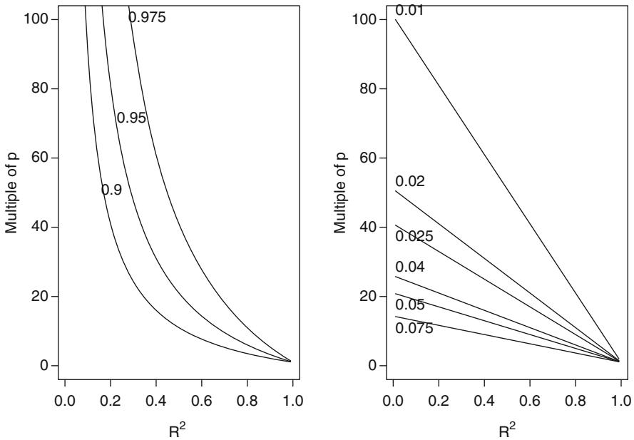
Fig. 4.1 Multiple of p that n must be to achieve a relative drop from R² to R² adj by the indicated relative factor (left panel, 3 factors) or absolute difference (right panel, 6 decrements)

low R² a 100:1 ratio of n : p may be required to prevent R² from dropping by more ¹ ¹⁰ or by an absolute amount of 0.01. A 15:1 rule would prevent R² from dropping by more than 0.075 for low R² (Figure 4.1).

4.5 Shrinkage

The term shrinkage is used in regression modeling to denote two ideas. The first meaning relates to the slope of a calibration plot, which is a plot of observed responses against predicted responsesk. When a dataset is used to fit the model parameters as well as to obtain the calibration plot, the usual estimation process will force the slope of observed versus predicted values to be one. When, however, parameter estimates are derived from one dataset and then applied to predict outcomes on an independent dataset, overfitting will cause the slope of the calibration plot (i.e., the shrinkage factor ) to be less than one, a result of regression to the mean. Typically, low predictions will be too low and high predictions too high. Predictions near the mean predicted value will usually be quite accurate. The second meaning of shrinkage is a statistical estimation method that preshrinks regression coefficients towards zero so that the calibration plot for new data will not need shrinkage as its calibration slope will be one.

We turn first to shrinkage as an adverse result of traditional modeling. In ordinary linear regression, we know that all of the coefficient estimates are exactly unbiased estimates of the true effect when the model fits. Isn’t the existence of shrinkage and overfitting implying that there is some kind of bias in the parameter estimates? The answer is no because each separate coefficient has the desired expectation. The problem lies in how we use the coefficients. We tend not to pick out coefficients at random for interpretation but we tend to highlight very small and very large coefficients.

A simple example may suffice. Consider a clinical trial with 10 randomly assigned treatments such that the patient responses for each treatment are normally distributed. We can do an ANOVA by fitting a multiple regression model with an intercept and nine dummy variables. The intercept is an unbiased estimate of the mean response for patients on the first treatment, and each of the other coefficients is an unbiased estimate of the difference in mean response between the treatment in question and the first treatment. βˆ ⁰ + βˆ ¹ is an unbiased estimate of the mean response for patients on the second treatment. But if we plotted the predicted mean response for patients against the observed responses from new data, the slope of this calibration plot would typically be smaller than one. This is because in making this plot we are not picking coefficients at random but we are sorting the coefficients into ascending order. The treatment group having the lowest sample mean response will usually have a higher mean in the future, and the treatment group having the highest sample mean response will typically have a lower mean in the future. The sample mean of the group having the highest sample mean is not an unbiased estimate of its population mean.

^k An even more stringent assessment is obtained by stratifying calibration curves by predictor settings.

As an illustration, let us draw 20 samples of size n = 50 from a uniform distribution for which the true mean is 0.5. Figure 4.2 displays the 20 means sorted into ascending order, similar to plotting Y versus Yˆ = Xβˆ based on least squares after sorting by Xβˆ. Bias in the very lowest and highest estimates is evident.

set.seed (123)
n ← 50
y ← runif (20*n)
group ← rep(1:20,each=n)
ybar ← tapply (y, group , mean)
ybar ← sort(ybar)
plot (1:20, ybar , type= ' n ' , axes= FALSE , ylim =c(.3 ,.7),
     xlab= ' Group ' , ylab= ' Group Mean ' )
lines (1:20, ybar)
points (1:20, ybar , pch=20, cex=.5)
axis (2)
axis (1, at =1:20, labels =FALSE )
for(j in 1:20) axis (1, at=j, labels =names (ybar )[j])
abline (h=.5 , col= gray(.85))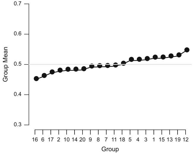

Fig. 4.2 Sorted means from 20 samples of size 50 from a uniform [0, 1] distribution. The reference line at 0.5 depicts the true population value of all of the means.

When we want to highlight a treatment that is not chosen at random (or a priori), the data-based selection of that treatment needs to be compensated for in the estimation process.l It is well known that the use of shrinkage

^l It is interesting that researchers are quite comfortable with adjusting P-values for post hoc selection of comparisons using, for example, the Bonferroni inequality, but they do not realize that post hoc selection of comparisons also biases point estimates.

methods such as the James–Stein estimator to pull treatment means toward the grand mean over all treatments results in estimates of treatment-specific means that are far superior to ordinary stratified means.176

Turning from a cell means model to the general case where predicted values are general linear combinations Xβˆ, the slope γ of properly transformed responses Y against Xβˆ (sorted into ascending order) will be less than one on new data. Estimation of the shrinkage coefficient γ allows quantification of the amount of overfitting present, and it allows one to estimate the likelihood that the model will reliably predict new observations. van Houwelingen and le Cessie [633, Eq. 77] provided a heuristic shrinkage estimate that has worked well in several examples:

\[ \hat{\gamma} = \frac{\text{model } \chi^2 - p}{\text{model } \chi^2}, \tag{4.3} \]

where p is the total degrees of freedom for the predictors and model χ² is ¹³ the likelihood ratio χ² statistic for testing the joint influence of all predictors simultaneously (see Section 9.3.1). For ordinary linear models, van Houwelingen and le Cessie proposed a shrinkage factor ˆγ that can be shown to equal n−p−1 n−1 R² adj ^R² , where the adjusted R² is given by ¹⁴

\[R\_{\rm adj}^2 = 1 - (1 - R^2) \frac{n - 1}{n - p - 1}. \tag{4.4}\]

For such linear models with an intercept β0, the shrunken estimate of β is

\[ \begin{aligned} \hat{\beta}\_0^s &= (1 - \hat{\gamma})\overline{Y} + \hat{\gamma}\hat{\beta}\_0 \\ \hat{\beta}\_j^s &= \hat{\gamma}\hat{\beta}\_j, j = 1, \dots, p,\end{aligned} \tag{4.5} \]

where Y is the mean of the response vector. Again, when stepwise fitting is used, the p in these equations is much closer to the number of candidate degrees of freedom rather than the number in the “final” model. See Section 5.3 ¹⁵ for methods of estimating γ using the bootstrap (p. 115) or cross-validation.

Now turn to the second usage of the term shrinkage. Just as clothing is sometimes preshrunk so that it will not shrink further once it is purchased, better calibrated predictions result when shrinkage is built into the estimation process in the first place. The object of shrinking regression coefficient estimates is to obtain a shrinkage coefficient of γ = 1 on new data. Thus by somewhat discounting βˆ we make the model underfitted on the data at hand (i.e., apparent γ < 1) so that on new data extremely low or high predictions are correct.

Ridge regression388, 633 is one technique for placing restrictions on the parameter estimates that results in shrinkage. A ridge parameter must be chosen to control the amount of shrinkage. Penalized maximum likelihood estimation,237, 272, 388, 639 a generalization of ridge regression, is a general shrinkage

procedure. A method such as cross-validation or optimization of a modified AIC must be used to choose an optimal penalty factor. An advantage of penalized estimation is that one can differentially penalize the more complex components of the model such as nonlinear or interaction effects. A drawback of ridge regression and penalized maximum likelihood is that the final model is difficult to validate unbiasedly since the optimal amount of shrinkage is usually determined by examining the entire dataset. Penalization is one of the best ways to approach the “too many variables, too little data” problem. See Section 9.10 for details.

4.6 Collinearity

When at least one of the predictors can be predicted well from the other predictors, the standard errors of the regression coefficient estimates can be inflated and corresponding tests have reduced power.217 In stepwise variable selection, collinearity can cause predictors to compete and make the selection of “important” variables arbitrary. Collinearity makes it difficult to estimate and interpret a particular regression coefficient because the data have little information about the effect of changing one variable while holding another (highly correlated) variable constant [101, Chap. 9]. However, collinearity does not affect the joint influence of highly correlated variables when tested simultaneously. Therefore, once groups of highly correlated predictors are identified, the problem can be rectified by testing the contribution of an entire set with a multiple d.f. test rather than attempting to interpret the coefficient or one d.f. test for a single predictor.

Collinearity does not affect predictions made on the same dataset used to estimate the model parameters or on new data that have the same degree of collinearity as the original data [470, pp. 379–381] as long as extreme extrapolation is not attempted. Consider as two predictors the total and LDL cholesterols that are highly correlated. If predictions are made at the same combinations of total and LDL cholesterol that occurred in the training data, no problem will arise. However, if one makes a prediction at an inconsistent combination of these two variables, the predictions may be inaccurate and have high standard errors.

When the ordinary truncated power basis is used to derive component variables for fitting linear and cubic splines, as was described earlier, the component variables can be very collinear. It is very unlikely that this will result in any problems, however, as the component variables are connected algebraically. Thus it is not possible for a combination of, for example, x and max(x − 10, 0) to be inconsistent with each other. Collinearity problems are then more likely to result from partially redundant subsets of predictors as in the cholesterol example above.

One way to quantify collinearity is with variance inflation factors or VIF, which in ordinary least squares are diagonals of the inverse of the X′ X matrix scaled to have unit variance (except that a column of 1s is retained corresponding to the intercept). Note that some authors compute VIF from the correlation matrix form of the design matrix, omitting the intercept. V IFⁱ is ¹/(1 ⁻ ^R² ⁱ ) where R² ⁱ is the squared multiple correlation coefficient between column i and the remaining columns of the design matrix. For models that are fitted with maximum likelihood estimation, the information matrix is scaled to correlation form, and VIF is the diagonal of the inverse of this scaled matrix.147, 654 Then the VIF are similar to those from a weighted correlation matrix of the original columns in the design matrix. Note that indexes such 16 as VIF are not very informative as some variables are algebraically connected to each other.

The SAS VARCLUS procedure539 and R varclus function can identify collinear predictors. Summarizing collinear variables using a summary score is more powerful and stable than arbitrary selection of one variable in a group of collinear variables (see the next section). ¹⁷

4.7 Data Reduction

The sample size need not be as large as shown in Table 4.1 if the model is to be validated independently and if you don’t care that the model may fail to validate. However, it is likely that the model will be overfitted and will not validate if the sample size does not meet the guidelines. Use of data reduction methods before model development is strongly recommended if the conditions in Table 4.1 are not satisfied, and if shrinkage is not incorporated into parameter estimation. Methods such as shrinkage and data reduction reduce the effective d.f. of the model, making it more likely for the model to validate on future data. Data reduction is aimed at reducing the number of parameters to estimate in the model, without distorting statistical inference for the parameters. This is accomplished by ignoring Y during data reduction. Manipulations of X in unsupervised learning may result in a loss of information for predicting Y , but when the information loss is small, the gain in power and reduction of overfitting more than offset the loss.

Some available data reduction methods are given below.

1. Use the literature to eliminate unimportant variables.
1. Eliminate variables whose distributions are too narrow.
1. Eliminate candidate predictors that are missing in a large number of subjects, especially if those same predictors are likely to be missing for future applications of the model.
1. Use a statistical data reduction method such as incomplete principal component regression, nonlinear generalizations of principal components such

as principal surfaces, sliced inverse regression, variable clustering, or ordi-18 nary cluster analysis on a measure of similarity between variables.

See Chapters 8 and 14 for detailed case studies in data reduction.

4.7.1 Redundancy Analysis

There are many approaches to data reduction. One rigorous approach involves removing predictors that are easily predicted from other predictors, using flexible parametric additive regression models. This approach is unlikely to result in a major reduction in the number of regression coefficients to estimate against Y , but will usually provide insights useful for later data reduction over and above the insights given by methods based on pairwise correlations instead of multiple R².

The Hmisc redun function implements the following redundancy checking algorithm.

Expand each continuous predictor into restricted cubic spline basis functions. Expand categorical predictors into dummy variables.
Use OLS to predict each predictor with all component terms of all remaining predictors (similar to what the Hmisc transcan function does). When the predictor is expanded into multiple terms, use the first canonical variatem.
Remove the predictor that can be predicted from the remaining set with the highest adjusted or regular R².
Predict all remaining predictors from their complement.
Continue in like fashion until no variable still in the list of predictors can be predicted with an R² or adjusted R² greater than a specified threshold or until dropping the variable with the highest R² (adjusted or ordinary) would cause a variable that was dropped earlier to no longer be predicted at the threshold from the now smaller list of predictors.

Special consideration must be given to categorical predictors. One way to consider a categorical variable redundant is if a linear combination of dummy variables representing it can be predicted from a linear combination of other variables. For example, if there were 4 cities in the data and each city’s rainfall was also present as a variable, with virtually the same rainfall reported for all observations for a city, city would be redundant given rainfall (or viceversa). If two cities had the same rainfall, ‘city’ might be declared redundant even though tied cities might be deemed non-redundant in another setting. A second, more stringent way to check for redundancy of a categorical predictor is to ascertain whether all dummy variables created from the predictor are individually redundant. The redun function implements both approaches.

¹⁹ Examples of use of redun are given in two case studies.

^m There is an option to force continuous variables to be linear when they are being predicted.

4.7.2 Variable Clustering

Although the use of subject matter knowledge is usually preferred, statistical clustering techniques can be useful in determining independent dimensions that are described by the entire list of candidate predictors. Once each dimension is scored (see below), the task of regression modeling is simplified, and one quits trying to separate the effects of factors that are measuring the same phenomenon. One type of variable clustering539 is based on a type of oblique-rotation principal component (PC) analysis that attempts to separate variables so that the first PC of each group is representative of that group (the first PC is the linear combination of variables having maximum variance subject to normalization constraints on the coefficients142, 144). Another approach, that of doing a hierarchical cluster analysis on an appropriate similarity matrix (such as squared correlations) will often yield the same results. For either approach, it is often advisable to use robust (e.g., rank-based) measures for continuous variables if they are skewed, as skewed variables can greatly affect ordinary correlation coefficients. Pairwise deletion of missing values is also advisable for this procedure—casewise deletion can result in a small biased sample. ²⁰

When variables are not monotonically related to each other, Pearson or Spearman squared correlations can miss important associations and thus are not always good similarity measures. A general and robust similarity measure is Hoeffding’s D, 295 which for two variables X and Y is a measure of the agreement between F(x, y) and G(x)H(y), where G, H are marginal cumulative distribution functions and F is the joint CDF. The D statistic will detect a wide variety of dependencies between two variables.

See pp. 330 and 458 for examples of variable clustering. ²¹

4.7.3 Transformation and Scaling Variables Without Using Y

Scaling techniques often allow the analyst to reduce the number of parameters to fit by estimating transformations for each predictor using only information about associations with other predictors. It may be advisable to cluster variables before scaling so that patterns are derived only from variables that are related. For purely categorical predictors, methods such as correspondence analysis (see, for example, [108,139,239,391,456]) can be useful for data reduction. Often one can use these techniques to scale multiple dummy variables into a few dimensions. For mixtures of categorical and continuous predictors, qualitative principal component analysis such as the maximum total variance (MTV) method of Young et al.456, 680 is useful. For the special case of representing a series of variables with one PC, the MTV method is quite easy to implement.

1. Compute P C1, the first PC of the variables to reduce X1,…,X^q using the correlation matrix of Xs.
1. Use ordinary linear regression to predict P C¹ on the basis of functions of the Xs, such as restricted cubic spline functions for continuous Xs or a series of dummy variables for polytomous Xs. The expansion of each X^j is regressed separately on P C1.
1. These separately fitted regressions specify the working transformations of each X.
1. Recompute P C¹ by doing a PC analysis on the transformed Xs (predicted values from the fits).
1. Repeat steps 2 to 4 until the proportion of variation explained by P C¹ reaches a plateau. This typically requires three to four iterations.

A transformation procedure that is similar to MTV is the maximum generalized variance (MGV) method due to Sarle [368, pp. 1267–1268]. MGV involves predicting each variable from (the current transformations of) all the other variables. When predicting variable i, that variable is represented as a set of linear and nonlinear terms (e.g., spline components). Analysis of canonical variates279 can be used to find the linear combination of terms for Xⁱ (i.e., find a new transformation for Xi) and the linear combination of the current transformations of all other variables (representing each variable as a single, transformed, variable) such that these two linear combinations have maximum correlation. (For example, if there are only two variables X¹ and X² represented as quadratic polynomials, solve for a, b, c, d such that aX¹ + bX² 1 has maximum correlation with cX² +dX² ² .) The process is repeated until the transformations converge. The goal of MGV is to transform each variable so that it is most similar to predictions from the other transformed variables. MGV does not use PCs (so one need not precede the analysis by variable clustering), but once all variables have been transformed, you may want to summarize them with the first PC.

The SAS PRINQUAL procedure of Kuhfeld368 implements the MTV and MGV methods, and allows for very flexible transformations of the predictors, including monotonic splines and ordinary cubic splines.

A very flexible automatic procedure for transforming each predictor in turn, based on all remaining predictors, is the ACE (alternating conditional expectation) procedure of Breiman and Friedman.68 Like SAS PROC PRIN-QUAL, ACE handles monotonically restricted transformations and categorical variables. It fits transformations by maximizing R² between one variable and a set of variables. It automatically transforms all variables, using the “super smoother”207 for continuous variables. Unfortunately, ACE does not handle missing values. See Chapter 16 for more about ACE.

It must be noted that at best these automatic transformation procedures generally find only marginal transformations, not transformations of each predictor adjusted for the effects of all other predictors. When adjusted transformations differ markedly from marginal transformations, only joint modeling of all predictors (and the response) will find the correct transformations.

Once transformations are estimated using only predictor information, the adequacy of each predictor’s transformation can be checked by graphical methods, by nonparametric smooths of transformed X^j versus Y , or by expanding the transformed X^j using a spline function. This approach of checking that transformations are optimal with respect to Y uses the response data, but it accepts the initial transformations unless they are significantly inadequate. If the sample size is low, or if P C¹ for the group of variables used in deriving the transformations is deemed an adequate summary of those variables, that P C¹ can be used in modeling. In that way, data reduction is accomplished two ways: by not using Y to estimate multiple coefficients for a single predictor, and by reducing related variables into a single score, after transforming them. See Chapter 8 for a detailed example of these scaling techniques.

4.7.4 Simultaneous Transformation and Imputation

As mentioned in Chapter 3 (p. 52) if transformations are complex or nonmonotonic, ordinary imputation models may not work. SAS PROC PRINQUAL implemented a method for simultaneously imputing missing values while solving for transformations. Unfortunately, the imputation procedure frequently converges to imputed values that are outside the allowable range of the data. This problem is more likely when multiple variables are missing on the same subjects, since the transformation algorithm may simply separate missings and nonmissings into clusters.

A simple modification of the MGV algorithm of PRINQUAL that simultaneously imputes missing values without these problems is implemented in the R function transcan. Imputed values are initialized to medians of continuous variables and the most frequent category of categorical variables. For continuous variables, transformations are initialized to linear functions. For categorical ones, transformations may be initialized to the identify function, to dummy variables indicating whether the observation has the most prevalent categorical value, or to random numbers. Then when using canonical variates to transform each variable in turn, observations that are missing on the current “dependent” variable are excluded from consideration, although missing values for the current set of “predictors” are imputed. Transformed variables are normalized to have mean 0 and standard deviation 1. Although categorical variables are scored using the first canonical variate, transcan has an option to use recursive partitioning to obtain imputed values on the original scale (Section 2.5) for these variables. It defaults to imputing categorical variables using the category whose predicted canonical score is closest to the predicted score.

transcan uses restricted cubic splines to model continuous variables. It does not implement monotonicity constraints. transcan automatically constrains imputed values (both on transformed and original scales) to be in the same range as non-imputed ones. This adds much stability to the resulting estimates although it can result in a boundary effect. Also, imputed values can optionally be shrunken using Eq. 4.5 to avoid overfitting when developing the imputation models. Optionally, missing values can be set to specified constants rather than estimating them. These constants are ignored during the transformation-estimation phasen. This technique has proved to be helpful when, for example, a laboratory test is not ordered because a physician thinks the patient has returned to normal with respect to the lab parameter measured by the test. In that case, it’s better to use a normal lab value for missings.

The transformation and imputation information created by transcan may be used to transform/impute variables in datasets not used to develop the transformation and imputation formulas. There is also an R function to create R functions that compute the final transformed values of each predictor given input values on the original scale.

As an example of non-monotonic transformation and imputation, consider a sample of 1000 hospitalized patients from the SUPPORTo study.352 Two mean arterial blood pressure measurements were set to missing.

require( Hmisc )
getHdata(support) # Get data frame from web site
heart.rate ← support$hrt
blood.pressure ← support$ meanbp
blood.pressure [400:401]

Mean Arterial Blood Pressure Day 3 [1] 151 136

blood.pressure [400:401] ← NA # Create two missings
d ← data.frame (heart.rate , blood.pressure)
par(pch=46) # Figure 4.3
w ← transcan (∼ heart.rate + blood.pressure , transformed =TRUE ,
              imputed =TRUE , show.na=TRUE , data=d)

Convergence criterion:2.901 0.035

0.007
Convergence in 4 iterations
R2 achieved in predicting each variable:
    heart.rate blood.pressure
        0.259 0.259
Adjusted R2:
    heart.rate blood.pressure
        0.254 0.253

ⁿ If one were to estimate transformations without removing observations that had these constants inserted for the current Y -variable, the resulting transformations would likely have a spike at Y = imputation constant.

^o Study to Understand Prognoses Preferences Outcomes and Risks of Treatments

4.7 Data Reduction 85

w$imputed$blood.pressure

400 401
132.4057 109.7741

t ← w$transformed
spe ← round (c( spearman( heart.rate , blood.pressure ),
                 spearman(t[, ' heart.rate ' ],
                           t[, ' blood.pressure ' ])), 2)

Fig. 4.3 Transformations fitted using transcan. Tick marks indicate the two imputed values for blood pressure.

plot(heart.rate , blood.pressure ) # Figure 4.4
plot(t[, ' heart.rate ' ], t[, ' blood.pressure ' ],
     xlab= ' Transformed hr ' , ylab= ' Transformed bp ' )

Spearman’s rank correlation ρ between pairs of heart rate and blood pressure was -0.02, because these variables each require U-shaped transformations. Using restricted cubic splines with five knots placed at default quantiles, transcan provided the transformations shown in Figure 4.3. Correlation between transformed variables is ρ = −0.13. The fitted transformations are similar to those obtained from relating these two variables to time until death.

4.7.5 Simple Scoring of Variable Clusters

If a subset of the predictors is a series of related dichotomous variables, a simpler data reduction strategy is sometimes employed. First, construct two

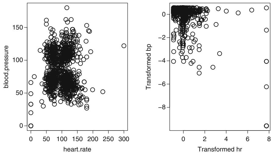
Fig. 4.4 The lower left plot contains raw data (Spearman ρ = −0.02); the lower right is a scatterplot of the corresponding transformed values (ρ = −0.13). Data courtesy of the SUPPORT study352.

new predictors representing whether any of the factors is positive and a count of the number of positive factors. For the ordinal count of the number of positive factors, score the summary variable to satisfy linearity assumptions as discussed previously. For the more powerful predictor of the two summary measures, test for adequacy of scoring by using all dichotomous variables as candidate predictors after adjusting for the new summary variable. A residual χ² statistic can be used to test whether the summary variable adequately captures the predictive information of the series of binary predictors.p This statistic will have degrees of freedom equal to one less than the number of binary predictors when testing for adequacy of the summary count (and hence will have low power when there are many predictors). Stratification by the summary score and examination of responses over cells can be used to suggest a transformation on the score.

Another approach to scoring a series of related dichotomous predictors is to have “experts” assign severity points to each condition and then to either sum these points or use a hierarchical rule that scores according to the condition with the highest points (see Section 14.3 for an example). The latter has the advantage of being easy to implement for field use. The adequacy of either type of scoring can be checked using tests of linearity in a regression modelq.

^p Whether this statistic should be used to change the model is problematic in view of model uncertainty.

^q The R function score.binary in the Hmisc package (see Section 6.2) assists in computing a summary variable from the series of binary conditions.

4.7.6 Simplifying Cluster Scores

If a variable cluster contains many individual predictors, parsimony may 22 sometimes be achieved by predicting the cluster score from a subset of its components (using linear regression or CART (Section 2.5), for example). Then a new cluster score is created and the response model is rerun with the new score in the place of the original one. If one constituent variable has a very high R² in predicting the original cluster score, the single variable may sometimes be substituted for the cluster score in refitting the model without loss of predictive discrimination.

Sometimes it may be desired to simplify a variable cluster by asking the question “which variables in the cluster are really the predictive ones?,” even though this approach will usually cause true predictive discrimination to suffer. For clusters that are retained after limited step-down modeling, the entire list of variables can be used as candidate predictors and the step-down process repeated. All variables contained in clusters that were not selected initially are ignored. A fair way to validate such two-stage models is to use a resampling method (Section 5.3) with scores for deleted clusters as candidate variables for each resample, along with all the individual variables in the clusters the analyst really wants to retain. A method called battery reduction can be used to delete variables from clusters by determining if a subset of the variables can explain most of the variance explained by P C¹ (see [142, Chapter 12] and445). This approach does not require examination of associations with Y . Battery reduction can also be used to find a set of individual variables that capture much of the information in the first k principal components. ²³

4.7.7 How Much Data Reduction Is Necessary?

In addition to using the sample size to degrees of freedom ratio as a rough guide to how much data reduction to do before model fitting, the heuristic shrinkage estimate in Equation 4.3 can also be informative. First, fit a full model with all candidate variables, nonlinear terms, and hypothesized interactions. Let p denote the number of parameters in this model, aside from any intercepts. Let LR denote the log likelihood ratio χ² for this full model. The estimated shrinkage is (LR − p)/LR. If this falls below 0.9, for example, we may be concerned with the lack of calibration the model may experience on new data. Either a shrunken estimator or data reduction is needed. A reduced model may have acceptable calibration if associations with Y are not used to reduce the predictors.

A simple method, with an assumption, can be used to estimate the target number of total regression degrees of freedom q in the model. In a “best case,” the variables removed to arrive at the reduced model would have no association with Y . The expected value of the χ² statistic for testing those

variables would then be p − q. The shrinkage for the reduced model is then on average [LR − (p − q) − q]/[LR − (p − q)]. Setting this ratio to be ≥ 0.9 and solving for q gives q ≤ (LR−p)/9. Therefore, reduction of dimensionality down to q degrees of freedom would be expected to achieve < 10% shrinkage. With these assumptions, there is no hope that a reduced model would have acceptable calibration unless LR > p+ 9. If the information explained by the omitted variables is less than one would expect by chance (e.g., their total χ² is extremely small), a reduced model could still be beneficial, as long as the conservative bound (LR−q)/LR ≥ 0.9 or q ≤ LR/10 were achieved. This conservative bound assumes that no χ² is lost by the reduction, that is that the final model ^χ² ^≈ LR. This is unlikely in practice. Had the ^p ⁻ ^q omitted variables had a larger ^χ² of 2(^p ⁻ ^q) (the break-even point for AIC), ^q must be ≤ (LR − 2p)/8.

As an example, suppose that a binary logistic model is being developed from a sample containing 45 events on 150 subjects. The 10:1 rule suggests we can analyze 4.5 degrees of freedom. The analyst wishes to analyze age, sex, and 10 other variables. It is not known whether interaction between age and sex exists, and whether age is linear. A restricted cubic spline is fitted with four knots, and a linear interaction is allowed between age and sex. These two variables then need 3 + 1 + 1 = 5 degrees of freedom. The other 10 variables are assumed to be linear and to not interact with themselves or age and sex. There is a total of 15 d.f. The full model with 15 d.f. has LR = 50. Expected shrinkage from this model is (50 − 15)/50 = 0.7. Since LR > 15 + 9 = 24, some reduction might yield a better validating model. Reduction to q = (50 − 15)/9 ≈ 4 d.f. would be necessary, assuming the reduced LR is about 50 − (15 − 4) = 39. In this case the 10:1 rule yields about the same value for q. The analyst may be forced to assume that age is linear, modeling 3 d.f. for age and sex. The other 10 variables would have to be reduced to a single variable using principal components or another scaling technique. The AIC-based calculation yields a maximum of 2.5 d.f.

If the goal of the analysis is to make a series of hypothesis tests (adjusting P-values for multiple comparisons) instead of to predict future responses, the full model would have to be used.

A summary of the various data reduction methods is given in Figure 4.5.

When principal component analysis or related methods are used for data reduction, the model may be harder to describe since internal coefficients are “hidden.” R code on p. 141 shows how an ordinary linear model fit can be used in conjunction with a logistic model fit based on principal components ²⁴ to draw a nomogram with axes for all predictors.

Goals	Reasons	Methods
Group predictors so that each group represents a single dimension that can be summarized with a sin gle score	• ↓ d.f. arising from mul tiple predictors • Make P C1 more reason able summary	Variable clustering • Sub ject matter knowl edge • Group predictors to maximize proportion of variance explained by of each group P C1 • Hierarchical clustering using a matrix of simi larity measures between predictors
Transform predictors	d.f. due to nonlin • ↓ ear and dummy variable components • Allows predictors to be optimally combined • Make P C1 more reason able summary • Use in customized model for imputing missing values on each predictor	• Maximum total vari ance on a group of re lated predictors • Canonical variates on the total set of predic tors
Score a group of predic tors	↓ d.f. for group to unity	• P C1 • Simple point scores
Multiple dimensional scoring of all predictors	d.f. for all predictors ↓ combined	Principal components 1, 2, , k, k com < p puted from all trans formed predictors

Fig. 4.5 Summary of Some Data Reduction Methods

4.8 Other Approaches to Predictive Modeling

The approaches recommended in this text are

fitting fully pre-specified models without deletion of “insignificant” predictors
using data reduction methods (masked to Y ) to reduce the dimensionality of the predictors and then fitting the number of parameters the data’s information content can support

• using shrinkage (penalized estimation) to fit a large model without worrying about the sample size.

Data reduction approaches covered in the last section can yield very interpretable, stable models, but there are many decisions to be made when using a two-stage (reduction/model fitting) approach. Newer single stage approaches are evolving. These new approaches, listed on the text’s web site, handle continuous predictors well, unlike recursive partitioning.

When data reduction is not required, generalized additive models277, 674 should also be considered.

4.9 Overly Influential Observations

Every observation should influence the fit of a regression model. It can be disheartening, however, if a significant treatment effect or the shape of a regression effect rests on one or two observations. Overly influential observations also lead to increased variance of predicted values, especially when variances are estimated by bootstrapping after taking variable selection into account. In some cases, overly influential observations can cause one to abandon a model, “change” the data, or get more data. Observations can be overly influential for several major reasons.

1. The most common reason is having too few observations for the complexity of the model being fitted. Remedies for this have been discussed in Sections 4.7 and 4.3.
1. Data transcription or data entry errors can ruin a model fit.
1. Extreme values of the predictor variables can have a great impact, even when these values are validated for accuracy. Sometimes the analyst may deem a subject so atypical of other subjects in the study that deletion of the case is warranted. On other occasions, it is beneficial to truncate measurements where the data density ends. In one dataset of 4000 patients and 2000 deaths, white blood count (WBC) ranged from 500 to 100,000 with .05 and .95 quantiles of 2755 and 26,700, respectively. Predictions from a linear spline function of WBC were sensitive to WBC > 60,000, for which there were 16 patients. There were 46 patients with WBC > 40,000. Predictions were found to be more stable when WBC was truncated at 40,000, that is, setting WBC to 40,000 if WBC > 40,000.
1. Observations containing disagreements between the predictors and the response can influence the fit. Such disagreements should not lead to discarding the observations unless the predictor or response values are erroneous as in Reason 3, or the analysis is made conditional on observations being unlike the influential ones. In one example a single extreme predictor value in a sample of size 8000 that was not on a straight line relationship with

the other (X, Y ) pairs caused a χ² of 36 for testing nonlinearity of the predictor. Remember that an imperfectly fitting model is a fact of life, and discarding the observations can inflate the model’s predictive accuracy. On rare occasions, such lack of fit may lead the analyst to make changes in the model’s structure, but ordinarily this is best done from the “ground up” using formal tests of lack of fit (e.g., a test of linearity or interaction).

Influential observations of the second and third kinds can often be detected by careful quality control of the data. Statistical measures can also be helpful. The most common measures that apply to a variety of regression models are leverage, DFBETAS, DFFIT, and DFFITS.

Leverage measures the capacity of an observation to be influential due to having extreme predictor values. Such an observation is not necessarily influential. To compute leverage in ordinary least squares, we define the hat matrix H given by

\[H = X(X^\prime X)^{-1}X^\prime. \tag{4.6}\]

H is the matrix that when multiplied by the response vector gives the predicted values, so it measures how an observation estimates its own predicted response. The diagonals hii of H are the leverage measures and they are not influenced by Y . It has been suggested47 that hii > 2(p + 1)/n signal a high leverage point, where p is the number of columns in the design matrix X aside from the intercept and n is the number of observations. Some believe that the distribution of hii should be examined for values that are higher than typical.

DFBETAS is the change in the vector of regression coefficient estimates upon deletion of each observation in turn, scaled by their standard errors.47 Since DFBETAS encompasses an effect for each predictor’s coefficient, DF-BETAS allows the analyst to isolate the problem better than some of the other measures. DFFIT is the change in the predicted Xβ when the observation is dropped, and DFFITS is DFFIT standardized by the standard error of the estimate of Xβ. In both cases, the standard error used for normalization is recomputed each time an observation is omitted. Some classify an observation as overly influential when |DFFITS| > 2 &(^p + 1)/(ⁿ ⁻ ^p ⁻ 1), while others prefer to examine the entire distribution of DFFITS to identify “outliers”.47

Section 10.7 discusses influence measures for the logistic model, which requires maximum likelihood estimation. These measures require the use of special residuals and information matrices (in place of X′ X).

If truly influential observations are identified using these indexes, careful thought is needed to decide how (or whether) to deal with them. Most important, there is no substitute for careful examination of the dataset before doing any analyses.99 Spence and Garrison [581, p. 16] feel that

Although the identification of aberrations receives considerable attention in most modern statistical courses, the emphasis sometimes seems to be on disposing of embarrassing data by searching for sources of technical error or minimizing the influence of inconvenient data by the application of resistant methods. Working scientists often find the most interesting aspect of the analysis inheres in the lack of fit rather than the fit itself.

4.10 Comparing Two Models

Frequently one wants to choose between two competing models on the basis of a common set of observations. The methods that follow assume that the performance of the models is evaluated on a sample not used to develop either one. In this case, predicted values from the model can usually be considered as a single new variable for comparison with responses in the new dataset. These methods listed below will also work if the models are compared using the same set of data used to fit each one, as long as both models have the same effective number of (candidate or actual) parameters. This requirement prevents us from rewarding a model just because it overfits the training sample (see Section 9.8.1 for a method comparing two models of differing complexity). The methods can also be enhanced using bootstrapping or cross-validation on a single sample to get a fair comparison when the playing field is not level, for example, when one model had more opportunity for fitting or overfitting the responses.

Some of the criteria for choosing one model over the other are

1. calibration (e.g., one model is well-calibrated and the other is not),
1. discrimination,
1. face validity,
1. measurement errors in required predictors,
1. use of continuous predictors (which are usually better defined than categorical ones),
1. omission of “insignificant” variables that nonetheless make sense as risk factors,
1. simplicity (although this is less important with the availability of computers), and
1. lack of fit for specific types of subjects.

Items 3 through 7 require subjective judgment, so we focus on the other aspects. If the purpose of the models is only to rank-order subjects, calibration is not an issue. Otherwise, a model having poor calibration can be dismissed outright. Given that the two models have similar calibration, discrimination should be examined critically. Various statistical indexes can quantify discrimination ability (e.g., R², model χ², Somers’ Dxy, Spearman’s ρ, area under ROC curve—see Section 10.8). Rank measures (Dxy, ρ, ROC area) only measure how well predicted values can rank-order responses. For example, predicted probabilities of 0.01 and 0.99 for a pair of subjects are no better than probabilities of 0.2 and 0.8 using rank measures, if the first subject had a lower response value than the second. Therefore, rank measures such as ROC area (c index), although fine for describing a given model, may not be very sensitive in choosing between two models118, 488, 493. This is especially true when the models are strong, as it is easier to move a rank correlation from 0.6 to 0.7 than it is to move it from 0.9 to 1.0. Measures such as R² and the model χ² statistic (calculated from the predicted and observed responses) are more sensitive. Still, one may not know how to interpret the added utility of a model that boosts the R² from 0.80 to 0.81.

Again given that both models are equally well calibrated, discrimination can be studied more simply by examining the distribution of predicted values Yˆ . Suppose that the predicted value is the probability that a subject dies. Then high-resolution histograms of the predicted risk distributions for the two models can be very revealing. If one model assigns 0.02 of the sample to a risk of dying above 0.9 while the other model assigns 0.08 of the sample to the high risk group, the second model is more discriminating. The worth of a model can be judged by how far it goes out on a limb while still maintaining good calibration. ²⁵

Frequently, one model will have a similar discrimination index to another model, but the likelihood ratio χ² statistic is meaningfully greater for one. Assuming corrections have been made for complexity, the model with the higher χ² usually has a better fit for some subjects, although not necessarily for the average subject. A crude plot of predictions from the first model against predictions from the second, possibly stratified by Y , can help describe the differences in the models. More specific analyses will determine the characteristics of subjects where the differences are greatest. Large differences may be caused by an omitted, underweighted, or improperly transformed predictor, among other reasons. In one example, two models for predicting hospital mortality in critically ill patients had the same discrimination index (to two decimal places). For the relatively small subset of patients with extremely low white blood counts or serum albumin, the model that treated these factors as continuous variables provided predictions that were very much different from a model that did not.

When comparing predictions for two models that may not be calibrated (from overfitting, e.g.), the two sets of predictions may be shrunk so as to not give credit for overfitting (see Equation 4.3).

Sometimes one wishes to compare two models that used the response variable differently, a much more difficult problem. For example, an investigator may want to choose between a survival model that used time as a continuous variable, and a binary logistic model for dead/alive at six months. Here, other considerations are also important (see Section 17.1). A model that predicts dead/alive at six months does not use the response variable effectively, and it provides no information on the chance of dying within three months.

When one or both of the models is fitted using least squares, it is useful to compare them using an error measure that was not used as the optimization criterion, such as mean absolute error or median absolute error. Mean

and median absolute errors are excellent measures for judging the value of a model developed without transforming the response to a model fitted after 26 transforming Y , then back-transforming to get predictions.

4.11 Improving the Practice of Multivariable Prediction

Standards for published predictive modeling and feature selection in highdimensional problems are not very high. There are several things that a good analyst can do to improve the situation.

1. Insist on validation of predictive models and discoveries, using rigorous internal validation based on resampling or using external validation.
1. Show collaborators that split-sample validation is not appropriate unless the number of subjects is huge
- This can be demonstrated by spliting the data more than once and seeing volatile results, and by calculating a confidence interval for the predictive accuracy in the test dataset and showing that it is very wide.
1. Run a simulation study with no real associations and show that associations are easy to find if a dangerous data mining procedure is used. Alternately, analyze the collaborator’s data after randomly permuting the Y vector and show some “positive” findings.
1. Show that alternative explanations are easy to posit. For example:
- The importance of a risk factor may disappear if 5 “unimportant” risk factors are added back to the model
- Omitted main effects can explain away apparent interactions.
- Perform a uniqueness analysis: attempt to predict the predicted values from a model derived by data torture from all of the features not used in the model. If one can obtain R² = 0.85 in predicting the “winning” feature signature (predicted values) from the “losing” features, the “winning” pattern is not unique and may be unreliable.

4.12 Summary: Possible Modeling Strategies

Some possible global modeling strategies are to

Use a method known not to work well (e.g., stepwise variable selection without penalization; recursive partitioning resulting in a single tree), document how poorly the model performs (e.g. using the bootstrap), and use the model anyway
Develop a black box model that performs poorly and is difficult to interpret (e.g., does not incorporate penalization)
Develop a black box model that performs well and is difficult to interpret
Develop interpretable approximations to the black box
Develop an interpretable model (e.g. give priority to additive effects) that performs well and is likely to perform equally well on future data from the same stream.

As stated in the Preface, the strategy emphasized in this text, stemming from the last philosophy, is to decide how many degrees of freedom can be “spent,” where they should be spent, and then to spend them. If statistical tests or confidence limits are required, later reconsideration of how d.f. are spent is not usually recommended. In what follows some default strategies are elaborated. These strategies are far from failsafe, but they should allow the reader to develop a strategy that is tailored to a particular problem. At the least these default strategies are concrete enough to be criticized so that statisticians can devise better ones.

4.12.1 Developing Predictive Models

The following strategy is generic although it is aimed principally at the development of accurate predictive models.

1. Assemble as much accurate pertinent data as possible, with wide distributions for predictor values. For survival time data, follow-up must be sufficient to capture enough events as well as the clinically meaningful phases if dealing with a chronic process.
1. Formulate good hypotheses that lead to specification of relevant candidate predictors and possible interactions. Don’t use Y (either informally using graphs, descriptive statistics, or tables, or formally using hypothesis tests or estimates of effects such as odds ratios) in devising the list of candidate predictors.
1. If there are missing Y values on a small fraction of the subjects but Y can be reliably substituted by a surrogate response, use the surrogate to replace the missing values. Characterize tendencies for Y to be missing using, for example, recursive partitioning or binary logistic regression. Depending on the model used, even the information on X for observations with missing Y can be used to improve precision of βˆ, so multiple imputation of Y can sometimes be effective. Otherwise, discard observations having missing Y .
1. Impute missing Xs if the fraction of observations with any missing Xs is not tiny. Characterize observations that had to be discarded. Special imputation models may be needed if a continuous X needs a non-monotonic transformation (p. 52). These models can simultaneously impute missing values while determining transformations. In most cases, multiply impute missing Xs based on other Xs and Y , and other available information about the missing data mechanism.
1. For each predictor specify the complexity or degree of nonlinearity that should be allowed (see Section 4.1). When prior knowledge does not indicate that a predictor has a linear effect on the property C(Y |X) (the property of the response that can be linearly related to X), specify the number of degrees of freedom that should be devoted to the predictor. The d.f. (or number of knots) can be larger when the predictor is thought to be more important in predicting Y or when the sample size is large.
1. If the number of terms fitted or tested in the modeling process (counting nonlinear and cross-product terms) is too large in comparison with the number of outcomes in the sample, use data reduction (ignoring Y ) until the number of remaining free variables needing regression coefficients is tolerable. Use the m/10 or m/15 rule or an estimate of likely shrinkage or overfitting (Section 4.7) as a guide. Transformations determined from the previous step may be used to reduce each predictor into 1 d.f., or the transformed variables may be clustered into highly correlated groups if more data reduction is required. Alternatively, use penalized estimation with the entire set of variables. This will also effectively reduce the total degrees of freedom.272
1. Use the entire sample in the model development as data are too precious to waste. If steps listed below are too difficult to repeat for each bootstrap or cross-validation sample, hold out test data from all model development steps that follow.
1. When you can test for model complexity in a very structured way, you may be able to simplify the model without a great need to penalize the final model for having made this initial look. For example, it can be advisable to test an entire group of variables (e.g., those more expensive to collect) and to either delete or retain the entire group for further modeling, based on a single P-value (especially if the P value is not between 0.05 and 0.2). Another example of structured testing to simplify the “initial” model is making all continuous predictors have the same number of knots k, varying k from 0 (linear), 3, 4, 5,… , and choosing the value of k that optimizes AIC. A composite test of all nonlinear effects in a model can also be used, and statistical inferences are not invalidated if the global test of nonlinearity yields P > 0.2 or so and the analyst deletes all nonlinear terms.
1. Make tests of linearity of effects in the model only to demonstrate to others that such effects are often statistically significant. Don’t remove insignificant effects from the model when tested separately by predictor. Any examination of the response that might result in simplifying the model needs to be accounted for in computing confidence limits and other statistics. It is preferable to retain the complexity that was prespecified in Step 5 regardless of the results of assessments of nonlinearity.

4.12 Summary: Possible Modeling Strategies 97

1. Check additivity assumptions by testing prespecified interaction terms. If the global test for additivity is significant or equivocal, all prespecified interactions should be retained in the model. If the test is decisive (e.g., P > 0.3), all interaction terms can be omitted, and in all likelihood there is no need to repeat this pooled test for each resample during model validation. In other words, one can assume that had the global interaction test been carried out for each bootstrap resample it would have been insignificant at the 0.05 level more than, say, 0.9 of the time. In this large P-value case the pooled interaction test did not induce an uncertainty in model selection that needed accounting.
1. Check to see if there are overly influential observations.
1. Check distributional assumptions and choose a different model if needed.
1. Do limited backwards step-down variable selection if parsimony is more important than accuracy.582 The cost of doing any aggressive variable selection is that the variable selection algorithm must also be included in a resampling procedure to properly validate the model or to compute confidence limits and the like.
1. This is the “final” model.
1. Interpret the model graphically (Section 5.1) and by examining predicted values and using appropriate significance tests without trying to interpret some of the individual model parameters. For collinear predictors obtain pooled tests of association so that competition among variables will not give misleading impressions of their total significance.
1. Validate the final model for calibration and discrimination ability, preferably using bootstrapping (see Section 5.3). Steps 9 to 13 must be repeated for each bootstrap sample, at least approximately. For example, if age was transformed when building the final model, and the transformation was suggested by the data using a fit involving age and age², each bootstrap repetition should include both age variables with a possible step-down from the quadratic to the linear model based on automatic significance testing at each step.
1. Shrink parameter estimates if there is overfitting but no further data reduction is desired, if shrinkage was not built into the estimation process.
1. When missing values were imputed, adjust final variance–covariance matrix for imputation wherever possible (e.g., using bootstrap or multiple imputation). This may affect some of the other results.
1. When all steps of the modeling strategy can be automated, consider using Faraway’s method186 to penalize for the randomness inherent in the multiple steps. ²⁷
1. Develop simplifications to the full model by approximating it to any desired degrees of accuracy (Section 5.5).

4.12.2 Developing Models for Effect Estimation

By effect estimation is meant point and interval estimation of differences in properties of the responses between two or more settings of some predictors, or estimating some function of these differences such as the antilog. In ordinary multiple regression with no transformation of Y such differences are absolute estimates. In regression involving log(Y ) or in logistic or proportional hazards models, effect estimation is, at least initially, concerned with estimation of relative effects. As discussed on pp. 4 and 224, estimation of absolute effects for these models must involve accurate prediction of overall response values, so the strategy in the previous section applies.

When estimating differences or relative effects, the bias in the effect estimate, besides being influenced by the study design, is related to how well subject heterogeneity and confounding are taken into account. The variance of the effect estimate is related to the distribution of the variable whose levels are being compared, and, in least squares estimates, to the amount of variation “explained” by the entire set of predictors. Variance of the estimated difference can increase if there is overfitting. So for estimation, the previous strategy largely applies.

The following are differences in the modeling strategy when effect estimation is the goal.

1. There is even less gain from having a parsimonious model than when developing overall predictive models, as estimation is usually done at the time of analysis. Leaving insignificant predictors in the model increases the likelihood that the confidence interval for the effect of interest has the stated coverage. By contrast, overall predictions are conditional on the values of all predictors in the model. The variance of such predictions is increased by the presence of unimportant variables, as predictions are still conditional on the particular values of these variables (Section 5.5.1) and cancellation of terms (which occurs when differences are of interest) does not occur.
1. Careful consideration of inclusion of interactions is still a major consideration for estimation. If a predictor whose effects are of major interest is allowed to interact with one or more other predictors, effect estimates must be conditional on the values of the other predictors and hence have higher variance.
1. A major goal of imputation is to avoid lowering the sample size because of missing values in adjustment variables. If the predictor of interest is the only variable having a substantial number of missing values, multiple imputation is less worthwhile, unless it corrects for a substantial bias caused by deletion of nonrandomly missing data.
1. The analyst need not be very concerned about conserving degrees of freedom devoted to the predictor of interest. The complexity allowed for this variable is usually determined by prior beliefs, with compromises that consider the bias-variance trade-off.
1. If penalized estimation is used, the analyst may wish to not shrink parameter estimates for the predictor of interest.
1. Model validation is not necessary unless the analyst wishes to use it to quantify the degree of overfitting.

4.12.3 Developing Models for Hypothesis Testing

A default strategy for developing a multivariable model that is to be used as a basis for hypothesis testing is almost the same as the strategy used for estimation.

1. There is little concern for parsimony. A full model fit, including insignificant variables, will result in more accurate P-values for tests for the variables of interest.
1. Careful consideration of inclusion of interactions is still a major consideration for hypothesis testing. If one or more predictors interacts with a variable of interest, either separate hypothesis tests are carried out over the levels of the interacting factors, or a combined “main effect + interaction” test is performed. For example, a very well–defined test is whether treatment is effective for any race group.
1. If the predictor of interest is the only variable having a substantial number of missing values, multiple imputation is less worthwhile. In some cases, multiple imputation may increase power (e.g., in ordinary multiple regression one can obtain larger degrees of freedom for error) but in others there will be little net gain. However, the test can be biased due to exclusion of nonrandomly missing observations if imputation is not done.
1. As before, the analyst need not be very concerned about conserving degrees of freedom devoted to the predictor of interest. The degrees of freedom allowed for this variable is usually determined by prior beliefs, with careful consideration of the trade-off between bias and power.
1. If penalized estimation is used, the analyst should not shrink parameter estimates for the predictors being tested.
1. Model validation is not necessary unless the analyst wishes to use it to quantify the degree of overfitting. This may shed light on whether there is overadjustment for confounders.

4.13 Further Reading

1 Some good general references that address modeling strategies are [216,269,476, 590].
2 Even though they used a generalized correlation index for screening variables and not for transforming them, Hall and Miller249 present a related idea, computing the ordinary R² against a cubic spline transformation of each potential predictor.
3 Simulation studies are needed to determine the effects of modifying the model based on assessments of “predictor promise.” Although it is unlikely that this strategy will result in regression coefficients that are biased high in absolute value, it may on some occasions result in somewhat optimistic standard errors and a slight elevation in type I error probability. Some simulation results may be found on the Web site. Initial promising findings for least squares models for two uncorrelated predictors indicate that the procedure is conservative in its estimation of σ² and in preserving type I error.
4 Verweij and van Houwelingen640 and Shao565 describe how cross-validation can be used in formulating a stopping rule. Luo et al.430 developed an approach to tuning forward selection by adding noise to Y .
5 Roecker528 compared forward variable selection (FS) and all possible subsets selection (APS) with full model fits in ordinary least squares. APS had a greater tendency to select smaller, less accurate models than FS. Neither selection technique was as accurate as the full model fit unless more than half of the candidate variables was redundant or unnecessary.
6 Wiegand668 showed that it is not very fruitful to try different stepwise algorithms and then to be comforted by agreements in some of the variables selected. It is easy for different stepwise methods to agree on the wrong set of variables.
7 Other results on how variable selection affects inference may be found in Hurvich and Tsai316 and Breiman [66, Section 8.1].
8 Goring et al.227 presented an interesting analysis of the huge bias caused by conditioning analyses on statistical significance in a high-dimensional genetics context.
9 Steyerberg et al.589 have comparisons of smoothly penalized estimators with the lasso and with several stepwise variable selection algorithms.
10 See Weiss,656 Faraway,186 and Chatfield100 for more discussions of the effect of not prespecifying models, for example, dependence of point estimates of effects on the variables used for adjustment.
11 Greenland241 provides an example in which overfitting a logistic model resulted in far too many predictors with P < 0.05.
12 See Peduzzi et al.486,487 for studies of the relationship between “events per variable” and types I and II error, accuracy of variance estimates, and accuracy of normal approximations for regression coefficient estimators. Their findings are consistent with those given in the text (but644 has a slightly different take). van der Ploeg et al.629 did extensive simulations to determine the events per variable ratio needed to avoid a drop-off (in an independent test sample) in more than 0.01 in the c-index, for a variety of predictive methods. They concluded that support vector machines, neural networks, and random forests needed far more events per variable to achieve freedom from overfitting than does logistic regression, and that recursive partitioning was not competitive. Logistic regression required between 20 and 50 events per variable to avoid overfitting. Different results might have been obtained had the authors used a proper accuracy score.
13 Copas [122, Eq. 8.5] adds 2 to the numerator of Equation 4.3 (see also [504,631]).
14 An excellent discussion about such indexes may be found in http://r.789695. n4.nabble.com/Adjusted-R-squared-formula-in-lm-td4656857.html where J. Lucke points out that R² tends to ^p ⁿ−¹ when the population ^R² is zero, but R² adj converges to zero.
15 Efron [173, Eq. 4.23] and van Houwelingen and le Cessie633 showed that the average expected optimism in a mean logarithmic quality score for a p-predictor binary logistic model is p/n. Taylor et al.600 showed that the ratio of variances for certain quantities is proportional to the ratio of the number of parameters in two models. Copas stated that “Shrinkage can be particularly marked when stepwise fitting is used: the shrinkage is then closer to that expected of the full regression rather than of the subset regression actually fitted.”122,504,631 Spiegelhalter,582 in arguing against variable selection, states that better prediction will often be obtained by fitting all candidate variables in the final model, shrinking the vector of regression coefficient estimates towards zero.
16 See Belsley [46, pp. 28–30] for some reservations about using VIF. 17 Friedman and Wall208 discuss and provide graphical devices for explaining suppression by a predictor not correlated with the response but that is correlated
with another predictor. Adjusting for a suppressor variable will increase the predictive discrimination of the model. Meinshausen453 developed a novel hierarchical approach to gauging the importance of collinear predictors.
18 For incomplete principal component regression see [101, 119, 120, 142, 144, 320, 325]. See396,686 for sparse principal component analysis methods in which constraints are applied to loadings so that some of them are set to zero. The latter reference provides a principal component method for binary data. See246 for a type of sparse principal component analysis that also encourages loadings to be similar for a group of highly correlated variables and allows for a type of variable clustering.See [390] for principal surfaces. Sliced inverse regression is described in [104, 119, 120, 189, 403, 404]. For material on variable clustering see [142, 144, 268, 441, 539]. A good general reference on cluster analysis is [634, Chapter 11]. de Leeuw and Mair in their R homals package [153] have one of the most general approaches to data reduction related to optimal scaling. Their approach includes nonlinear principal component analysis among several other multivariate analyses.
19 The redundancy analysis described here is related to principal variables448 but is faster.
20 Meinshausen453 developed a method of testing the importance of competing (collinear) variables using an interesting automatic clustering procedure.
21 The R ClustOfVar package by Marie Chavent, Vanessa Kuentz, Benoit Liquet, and Jerome Saracco generalizes variable clustering and explicitly handles a mixture of quantitative and categorical predictors. It also implements bootstrap cluster stability analysis.
22 Principal components are commonly used to summarize a cluster of variables. Vines643 developed a method to constrain the principal component coefficients to be integers without much loss of explained variability.
23 Jolliffe324 presented a way to discard some of the variables making up principal components. Wang and Gehan649 presented a new method for finding subsets of predictors that approximate a set of principal components, and surveyed other methods for simplifying principal components.
24 See D’Agostino et al.144 for excellent examples of variable clustering (including a two-stage approach) and other data reduction techniques using both statistical methods and subject-matter expertise.
25 Cook118 and Pencina et al.490,492,493 present an approach for judging the added value of new variables that is based on evaluating the extent to which the new information moves predicted probabilities higher for subjects having events and lower for subjects not having events. But see292,592.
26 The Hmisc abs.error.pred function computes a variety of accuracy measures based on absolute errors.
27 Shen et al.567 developed an “optimal approximation” method to make correct inferences after model selection.

4.14 Problems

Analyze the SUPPORT dataset (getHdata(support)) as directed below to relate selected variables to total cost of the hospitalization. Make sure this response variable is utilized in a way that approximately satisfies the assumptions of normality-based multiple regression so that statistical inferences will be accurate. See problems at the end of Chapters 3 and 7 of the text for more information. Consider as predictors mean arterial blood pressure, heart rate, age, disease group, and coma score.

1. Do an analysis to understand interrelationships among predictors, and find optimal scaling (transformations) that make the predictors better relate to each other (e.g., optimize the variation explained by the first principal component).
1. Do a redundancy analysis of the predictors, using both a less stringent and a more stringent approach to assessing the redundancy of the multiple-level variable disease group.
1. Do an analysis that helps one determine how many d.f. to devote to each predictor.
1. Fit a model, assuming the above predictors act additively, but do not assume linearity for the age and blood pressure effects. Use the truncated power basis for fitting restricted cubic spline functions with 5 knots. Estimate the shrinkage coefficient ˆγ.
1. Make appropriate graphical diagnostics for this model.
1. Test linearity in age, linearity in blood pressure, and linearity in heart rate, and also do a joint test of linearity simultaneously in all three predictors.
1. Expand the model to not assume additivity of age and blood pressure. Use a tensor natural spline or an appropriate restricted tensor spline. If you run into any numerical difficulties, use 4 knots instead of 5. Plot in an interpretable fashion the estimated 3-D relationship between age, blood pressure, and cost for a fixed disease group.
1. Test for additivity of age and blood pressure. Make a joint test for the overall absence of complexity in the model (linearity and additivity simultaneously).

Chapter 5 Describing, Resampling, Validating, and Simplifying the Model

5.1 Describing the Fitted Model

5.1.1 Interpreting Effects

Before addressing issues related to describing and interpreting the model and its coefficients, one can never apply too much caution in attempting to interpret results in a causal manner. Regression models are excellent tools for estimating and inferring associations between an X and Y given that the “right” variables are in the model. Any ability of a model to provide causal inference rests entirely on the faith of the analyst in the experimental design, completeness of the set of variables that are thought to measure confounding and are used for adjustment when the experiment is not randomized, lack of important measurement error, and lastly the goodness of fit of the model.

The first line of attack in interpreting the results of a multivariable analysis is to interpret the model’s parameter estimates. For simple linear, additive models, regression coefficients may be readily interpreted. If there are interactions or nonlinear terms in the model, however, simple interpretations are usually impossible. Many programs ignore this problem, routinely printing such meaningless quantities as the effect of increasing age² by one day while holding age constant. A meaningful age change needs to be chosen, and connections between mathematically related variables must be taken into account. These problems can be solved by relying on predicted values and differences between predicted values.

Even when the model contains no nonlinear effects, it is difficult to compare regression coefficients across predictors having varying scales. Some analysts like to gauge the relative contributions of different predictors on a common scale by multiplying regression coefficients by the standard deviations of the predictors that pertain to them. This does not make sense for nonnormally distributed predictors (and regression models should not need

^© Springer International Publishing Switzerland 2015 F.E. Harrell, Jr., Regression Modeling Strategies, Springer Series in Statistics, DOI 10.1007/978-3-319-19425-7 5

to make assumptions about the distributions of predictors). When a predictor is binary (e.g., sex), the standard deviation makes no sense as a scaling factor as the scale would depend on the prevalence of the predictor.a ¹

It is more sensible to estimate the change in Y when X^j is changed by an amount that is subject-matter relevant. For binary predictors this is a change from 0 to 1. For many continuous predictors the interquartile range is a reasonable default choice. If the 0.25 and 0.75 quantiles of X^j are g and h, linearity holds, and the estimated coefficient of X^j is b; b × (h − g) is the effect of increasing X^j by h − g units, which is a span that contains half of the sample values of Xj.

For the more general case of continuous predictors that are monotonically but not linearly related to Y , a useful point summary is the change in Xβ when the variable changes from its 0.25 quantile to its 0.75 quantile. For models for which exp(Xβ) is meaningful, antilogging the predicted change in Xβ results in quantities such as interquartile-range odds and hazards ratios. When the variable is involved in interactions, these ratios are estimated separately for various levels of the interacting factors. For categorical predictors, ordinary effects are computed by comparing each level of the predictor with a reference level. See Section 10.10 and Chapter 11 for tabular and graphical ² examples of this approach.

The model can be described using partial effect plots by plotting each X against Xβˆ holding other predictors constant. Modified versions of such plots, by nonlinearly rank-transforming the predictor axis, can show the relative importance of a predictor336.

For an X that interacts with other factors, separate curves are drawn on the same graph, one for each level of the interacting factor.

Nomograms40, 254, 339, 427 ³ provide excellent graphical depictions of all the variables in the model, in addition to enabling the user to obtain predicted values manually. Nomograms are especially good at helping the user envision ⁴ interactions. See Section 10.10 and Chapter 11 for examples.

5.1.2 Indexes of Model Performance

5.1.2.1 Error Measures

Care must be taken in the choice of accuracy scores to be used in validation. Indexes can be broken down into three main areas.

Central tendency of prediction errors: These measures include mean absolute differences, mean squared differences, and logarithmic scores. An absolute measure is mean ^|^Y ⁻ ^Y^ˆ ^|. The mean squared error is a commonly used and sensitive measure if there are no outliers. For the special case

^a The s.d. of a binary variable is, aside from a multiplier of ⁿ ⁿ−¹ , equal to &a(1 ⁻ ^a), where a is the proportion of ones.

where Y is binary, such a measure is the Brier score, which is a quadratic proper scoring rule that combines calibration and discriminationb. The logarithmic proper scoring rules (related to average log-likelihood) is even more sensitive but can be harder to interpret and can be destroyed by a single predicted probability of 0 or 1 that was incorrect.

Discrimination measures: A measure of pure discrimination is a rank correlation of Yˆ and Y , including Spearman’s ρ, Kendall’s τ, and Somers’ Dxy. When ^Y is binary, ^Dxy = 2 ^× (^c ⁻ ¹ ² ) where c is the concordance probability or area under the receiver operating characteristic curve, a linear translation of the Wilcoxon-Mann-Whitney statistic. R² is mostly a measure of discrimination, and R² adj is is a good overfitting-corrected measure, if the model is pre-specified. See Section 10.8 for more information about rank-based measures.
Discrimination measures based on variation in Yˆ : These include the regression sum of squares and the g–Index (see below).
Calibration measures: These assess absolute prediction accuracy. Calibration–in–the–large compares the average Yˆ with the average Y . A high-resolution calibration curve or calibration–in–the–small assesses the absolute forecast accuracy of predictions at individual levels of Yˆ . When the calibration curve is linear, this can be summarized by the calibration slope and intercept. A more general approach uses the loess nonparametric smoother to estimate the calibration curve37. For any shape of calibration curve, errors can be summarized by quantities such as the maximum absolute calibration error, mean absolute calibration error, and 0.9 quantile of calibration error.

The g-index is a new measure of a model’s predictive discrimination based only on Xβˆ = Yˆ that applies quite generally. It is based on Gini’s mean difference for a variable Z, which is the mean over all possible i ̸= j of |Zⁱ − Z^j |. The g-index is an interpretable, robust, and highly efficient measure of variation. For example, when predicting systolic blood pressure, g = 11mmHg represents a typical difference in Yˆ . g is independent of censoring and other complexities. For models in which the anti-log of a difference in Yˆ represents meaningful ratios (e.g., odds ratios, hazard ratios, ratio of medians), g^r can be defined as exp(g). For models in which Yˆ can be turned into a probability ⁵ estimate (e.g., logistic regression), g^p is defined as Gini’s mean difference of Pˆ. These g–indexes represent e.g. “typical” odds ratios, and “typical” risk differences. Partial g indexes can also be defined. More details may be found in the documentation for the R rms package’s gIndex function.

^b There are decompositions of the Brier score into discrimination and calibration components.

5.2 The Bootstrap

When one assumes that a random variable Y has a certain population distribution, one can use simulation or analytic derivations to study how a statistical estimator computed from samples from this distribution behaves. For example, when Y has a log-normal distribution, the variance of the sample median for a sample of size n from that distribution can be derived analytically. Alternatively, one can simulate 500 samples of size n from the lognormal distribution, compute the sample median for each sample, and then compute the sample variance of the 500 sample medians. Either case requires knowledge of the population distribution function.

Efron’s bootstrap150, 177, 178 is a general-purpose technique for obtaining estimates of the properties of statistical estimators without making assumptions about the distribution giving rise to the data. Suppose that a random variable Y comes from a cumulative distribution function F(y) = Prob{Y ≤ y} and that we have a sample of size n from this unknown distribution, Y1, Y2,…,Yn. The basic idea is to repeatedly simulate a sample of size n from F, computing the statistic of interest, and assessing how the statistic behaves over B repetitions. Not having F at our disposal, we can estimate F by the empirical cumulative distribution function

\[F\_n(y) = \frac{1}{n} \sum\_{i=1}^n [Y\_i \le y]. \tag{5.1}\]

Fⁿ corresponds to a density function that places probability 1/n at each observed datapoint (k/n if that point were duplicated k times and its value listed only once).

As an example, consider a random sample of size n = 30 from a normal distribution with mean 100 and standard deviation 10. Figure 5.1 shows the population and empirical cumulative distribution functions.

Now pretend that Fn(y) is the original population distribution F(y). Sampling from Fⁿ is equivalent to sampling with replacement from the observed data Y1,…,Yn. For large n, the expected fraction of original datapoints that are selected for each bootstrap sample is 1 ⁻ ^e−¹ = 0.632. Some points are selected twice, some three times, a few four times, and so on. We take B samples of size n with replacement, with B chosen so that the summary measure ⁶ of the individual statistics is nearly as good as taking B = ∞. The bootstrap is based on the fact that the distribution of the observed differences between a resampled estimate of a parameter of interest and the original estimate of the parameter from the whole sample tells us about the distribution of unobservable differences between the original estimate and the unknown population value of the parameter.

As an example, consider the data (1, 5, 6, 7, 8, 9) and suppose that we would like to obtain a 0.80 confidence interval for the population median, as well as an estimate of the population expected value of the sample median (the latter

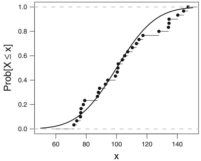
Fig. 5.1 Empirical and population cumulative distribution function

is only used to estimate bias in the sample median). The first 20 bootstrap samples (after sorting data values) and the corresponding sample medians are shown in Table 5.1.

For a given number B of bootstrap samples, our estimates are simply the sample 0.1 and 0.9 quantiles of the sample medians, and the mean of the sample medians. Not knowing how large B should be, we could let B range from, say, 50 to 1000, stopping when we are sure the estimates have converged. In the left plot of Figure 5.2, B varies from 1 to 400 for the mean (10 to 400 for the quantiles). It can be seen that the bootstrap estimate of the population mean of the sample median can be estimated satisfactorily when B > 50. For the lower and upper limits of the 0.8 confidence interval for the population median Y , B must be at least 200. For more extreme confidence limits, B must be higher still.

For the final set of 400 sample medians, a histogram (right plot in Figure 5.2) can be used to assess the form of the sampling distribution of the sample median. Here, the distribution is almost normal, although there is a slightly heavy left tail that comes from the data themselves having a heavy left tail. For large samples, sample medians are normally distributed for a wide variety of population distributions. Therefore we could use bootstrapping to estimate the variance of the sample median and then take ±1.28 standard errors as a 0.80 confidence interval. In other cases (e.g., regression coefficient estimates for certain models), estimates are asymmetrically distributed, and the bootstrap quantiles are better estimates than confidence intervals that are based on a normality assumption. Note that because sample quantiles are more or less restricted to equal one of the values in the sample, the boot-

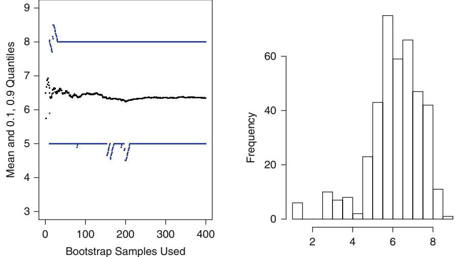
Fig. 5.2 Estimating properties of sample median using the bootstrap

Bootstrap Sample	Sample Median
1 6 6 7 8 9	6.5
1 5 5 5 6 8	5.0
5 7 8 9 9 9	8.5
7 7 7 8 8 9	7.5
1 5 7 7 9 9	7.0
1 5 6 6 7 8	6.0
7 8 8 8 8 8	8.0
5 5 5 7 9 9	6.0
1 5 5 7 7 9	6.0
1 5 5 7 7 8	6.0
1 1 5 5 7 7	5.0
1 1 5 5 7 8	5.0
1 5 5 7 7 8	6.0
1 5 6 7 8 8	6.5
1 5 6 7 9 9	6.5
6 6 7 7 8 9	7.0
1 5 7 8 8 9	7.5
6 6 8 9 9 9	8.5
1 1 5 5 6 9	5.0
1 6 8 9 9 9	8.5

Table 5.1 First 20 bootstrap samples

strap distribution is discrete and can be dependent on a small number of outliers. For this reason, bootstrapping quantiles does not work particularly well for small samples [150, pp. 41–43].

The method just presented for obtaining a nonparametric confidence interval for the population median is called the bootstrap percentile method. It is the simplest but not necessarily the best performing bootstrap method. 7

In this text we use the bootstrap primarily for computing statistical estimates that are much different from standard errors and confidence intervals, namely, estimates of model performance.

5.3 Model Validation

5.3.1 Introduction

The surest method to have a model fit the data at hand is to discard much of the data. A p-variable fit to p + 1 observations will perfectly predict Y as long as no two observations have the same Y . Such a model will, however, yield predictions that appear almost random with respect to responses on a different dataset. Therefore, unbiased estimates of predictive accuracy are essential.

Model validation is done to ascertain whether predicted values from the model are likely to accurately predict responses on future subjects or subjects not used to develop our model. Three major causes of failure of the ⁸ model to validate are overfitting, changes in measurement methods/changes in definition of categorical variables, and major changes in subject inclusion criteria.

There are two major modes of model validation, external and internal. The most stringent external validation involves testing a final model developed in one country or setting on subjects in another country or setting at another time. This validation would test whether the data collection instrument was translated into another language properly, whether cultural differences make earlier findings nonapplicable, and whether secular trends have changed associations or base rates. Testing a finished model on new subjects from the ⁹ same geographic area but from a different institution as subjects used to fit the model is a less stringent form of external validation. The least stringent form of external validation involves using the first m of n observations for model training and using the remaining n − m observations as a test sample. This is very similar to data-splitting (Section 5.3.3). For details about methods for external validation see the R val.prob and val.surv functions in the rms package.

Even though external validation is frequently favored by non-statisticians, it is often problematic. Holding back data from the model-fitting phase results in lower precision and power, and one can increase precision and learn more about geographic or time differences by fitting a unified model to the entire subject series including, for example, country or calendar time as a main effect and/or as an interacting effect. Indeed one could use the following working definition of external validation: validation of a prediction tool using data that were not available when the tool needed to be completed. An alternate definition could be taken as the validation of a prediction tool by an independent research team.

One suggested hierarchy of the quality of various validation methods is as follows, ordered from worst to best.

1. Attempting several validations (internal or external) and reporting only the one that “worked”
1. Reporting apparent performance on the training dataset (no validation)
1. Reporting predictive accuracy on an undersized independent test sample
1. Internal validation using data-splitting where at least one of the training and test samples is not huge and the investigator is not aware of the arbitrariness of variable selection done on a single sample
1. Strong internal validation using 100 repeats of 10-fold cross-validation or several hundred bootstrap resamples, repeating all analysis steps involving Y afresh at each re-sample and the arbitrariness of selected “important variables” is reported (if variable selection is used)
1. External validation on a large test sample, done by the original research team
1. Re-analysis by an independent research team using strong internal validation of the original dataset
1. External validation using new test data, done by an independent research team
1. External validation using new test data generated using different instruments/technology, done by an independent research team

Internal validation involves fitting and validating the model by carefully using one series of subjects. One uses the combined dataset in this way to estimate the likely performance of the final model on new subjects, which after all is often of most interest. Most of the remainder of Section 5.3 deals with internal validation.

5.3.2 Which Quantities Should Be Used in Validation?

For ordinary multiple regression models, the R² index is a good measure of the model’s predictive ability, especially for the purpose of quantifying drop-off in predictive ability when applying the model to other datasets. R² is biased, however. For example, if one used nine predictors to predict outcomes of 10 subjects, R² = 1.0 but the R² that will be achieved on future

subjects will be close to zero. In this case, dramatic overfitting has occurred. The adjusted R² (Equation 4.4) solves this problem, at least when the model has been completely prespecified and no variables or parameters have been “screened” out of the final model fit. That is, R² adj is only valid when p in its formula is honest— when it includes all parameters ever examined (formally or informally, e.g., using graphs or tables) whether these parameters are in the final model or not.

Quite often we need to validate indexes other than R² for which adjustments for p have not been created.c We also need to validate models containing “phantom degrees of freedom” that were screened out earlier, formally or informally. For these purposes, we obtain nearly unbiased estimates of R² or other indexes using data splitting, cross-validation, or the bootstrap. The bootstrap provides the most precise estimates.

The g–index is another discrimination measure to validate. But g and R² measures only one aspect of predictive ability. In general, there are two major aspects of predictive accuracy that need to be assessed. As discussed in Section 4.5, calibration or reliability is the ability of the model to make unbiased estimates of outcome. Discrimination is the model’s ability to separate subjects’ outcomes. Validation of the model is recommended even when a data reduction technique is used. This is a way to ensure that the model was not overfitted or is otherwise inaccurate.

5.3.3 Data-Splitting

The simplest validation method is one-time data-splitting. Here a dataset is split into training (model development) and test (model validation) samples by a random process with or without balancing distributions of the response and predictor variables in the two samples. In some cases, a chronological split is used so that the validation is prospective. The model’s calibration and discrimination are validated in the test set.

In ordinary least squares, calibration may be assessed by, for example, plotting Y against Yˆ . Discrimination here is assessed by R² and it is of interest in comparing R² in the training sample with that achieved in the test sample. A drop in R² indicates overfitting, and the absolute R² in the test sample is an unbiased estimate of predictive discrimination. Note that in extremely overfitted models, R² in the test set can be negative, since it is computed on “frozen” intercept and regression coefficients using the formula 1−SSE/SST , where SSE is the error sum of squares, SST is the total sum

^c For example, in the binary logistic model, there is a generalization of R² available, but no adjusted version. For logistic models we often validate other indexes such as the ROC area or rank correlation between predicted probabilities and observed outcomes. We also validate the calibration accuracy of Yˆ in predicting Y .

of squares, and SSE can be greater than SST (when predictions are worse ¹⁰ than the constant predictor Y ).

To be able to validate predictions from the model over an entire test sample (without validating it separately in particular subsets such as in males and females), the test sample must be large enough to precisely fit a model containing one predictor. For a study with a continuous uncensored response variable, the test sample size should ordinarily be ≥ 100 at a bare minimum. For survival time studies, the test sample should at least be large enough to contain a minimum of 100 outcome events. For binary outcomes, the test sample should contain a bare minimum of 100 subjects in the least frequent outcome category. Once the size of the test sample is determined, the remaining portion of the original sample can be used as a training sample. Even with these test sample sizes, validation of extreme predictions is difficult.

Data-splitting has the advantage of allowing hypothesis tests to be confirmed in the test sample. However, it has the following disadvantages.

1. Data-splitting greatly reduces the sample size for both model development and model testing. Because of this, Roecker528 found this method “appears to be a costly approach, both in terms of predictive accuracy of the fitted model and the precision of our estimate of the accuracy.” Breiman [66, Section 1.3] found that bootstrap validation on the original sample was as efficient as having a separate test sample twice as large36.
1. It requires a larger sample to be held out than cross-validation (see below) to be able to obtain the same precision of the estimate of predictive accuracy.
1. The split may be fortuitous; if the process were repeated with a different split, different assessments of predictive accuracy may be obtained.
1. Data-splitting does not validate the final model, but rather a model developed on only a subset of the data. The training and test sets are recombined for fitting the final model, which is not validated.
1. Data-splitting requires the split before the first analysis of the data. With other methods, analyses can proceed in the usual way on the complete dataset. Then, after a “final” model is specified, the modeling process is rerun on multiple resamples from the original data to mimic the process that produced the “final” model.

5.3.4 Improvements on Data-Splitting: Resampling

Bootstrapping, jackknifing, and other resampling plans can be used to obtain nearly unbiased estimates of model performance without sacrificing sample size. These methods work when either the model is completely specified except for the regression coefficients, or all important steps of the modeling process, especially variable selection, are automated. Only then can each bootstrap replication be a reflection of all sources of variability in modeling. Note that most analyses involve examination of graphs and testing for lack of model fit, with many intermediate decisions by the analyst such as simplification of interactions. These processes are difficult to automate. But variable selection alone is often the greatest source of variability because of multiple comparison problems, so the analyst must go to great lengths to bootstrap or jackknife variable selection.

The ability to study the arbitrariness of how a stepwise variable selection algorithm selects “important” factors is a major benefit of bootstrapping. A useful display is a matrix of blanks and asterisks, where an asterisk is placed in column x of row i if variable x is selected in bootstrap sample i (see p. 263 for an example). If many variables appear to be selected at random, the analyst may want to turn to a data reduction method rather than using stepwise selection (see also [541]).

Cross-validation is a generalization of data-splitting that solves some of the problems of data-splitting. Leave-out-one cross-validation, 565, 633 the limit of cross-validation, is similar to jackknifing.675 Here one observation is omitted from the analytical process and the response for that observation is predicted using a model derived from the remaining n − 1 observations. The process is repeated n times to obtain an average accuracy. Efron172 reports that grouped cross-validation is more accurate; here groups of k observations are omitted at a time. Suppose, for example, that 10 groups are used. The original dataset is divided into 10 equal subsets at random. The first 9 subsets are used to develop a model (transformation selection, interaction testing, stepwise variable selection, etc. are all done). The resulting model is assessed for accuracy on the remaining 1/10th of the sample. This process is repeated at least 10 times to get an average of 10 indexes such as R². ¹¹

A drawback of cross-validation is the choice of the number of observations to hold out from each fit. Another is that the number of repetitions needed to achieve accurate estimates of accuracy often exceeds 200. For example, one may have to omit ¹ ¹⁰ th of the sample 500 times to accurately estimate the index of interest Thus the sample would need to be split into tenths 50 times. ¹² Another possible problem is that cross-validation may not fully represent the variability of variable selection. If 20 subjects are omitted each time from a sample of size 1000, the lists of variables selected from each training sample of size 980 are likely to be much more similar than lists obtained from fitting independent samples of 1000 subjects. Finally, as with data-splitting, crossvalidation does not validate the full 1000-subject model.

An interesting way to study overfitting could be called the randomization method. Here we ask the question “How well can the response be predicted when we use our best procedure on random responses when the predictive accuracy should be near zero?” The better the fit on random Y , the worse the overfitting. The method takes a random permutation of the response variable and develops a model with optional variable selection based on the original X and permuted Y . Suppose this yields R² = .2 for the fitted sample. Apply the

fit to the original data to estimate optimism. If overfitting is not a problem, ¹³ R² would be the same for both fits and it will ordinarily be very near zero.

5.3.5 Validation Using the Bootstrap

Efron,172, 173 Efron and Gong,175 Gong,224 Efron and Tibshirani,177, 178 Linnet,416 and Breiman66 describe several bootstrapping procedures for obtaining nearly unbiased estimates of future model performance without holding back data when making the final estimates of model parameters. With the “simple bootstrap” [178, p. 247], one repeatedly fits the model in a bootstrap sample and evaluates the performance of the model on the original sample. The estimate of the likely performance of the final model on future data is estimated by the average of all of the indexes computed on the original sample.

Efron showed that an enhanced bootstrap estimates future model performance more accurately than the simple bootstrap. Instead of estimating an accuracy index directly from averaging indexes computed on the original sample, the enhanced bootstrap uses a slightly more indirect approach by estimating the bias due to overfitting or the “optimism” in the final model fit. After the optimism is estimated, it can be subtracted from the index of accuracy derived from the original sample to obtain a bias-corrected or overfitting-corrected estimate of predictive accuracy. The bootstrap method is as follows. From the original X and Y in the sample of size n, draw a sample with replacement also of size n. Derive a model in the bootstrap sample and apply it without change to the original sample. The accuracy index from the bootstrap sample minus the index computed on the original sample is an estimate of optimism. This process is repeated for 100 or so bootstrap replications to obtain an average optimism, which is subtracted from the final ¹⁴ model fit’s apparent accuracy to obtain the overfitting-corrected estimate.

Note that bootstrapping validates the process that was used to fit the original model (as does cross-validation). It provides an estimate of the expected value of the optimism, which when subtracted from the original index, pro-¹⁵ vides an estimate of the expected bias-corrected index. If stepwise variable selection is part of the bootstrap process (as it must be if the final model is developed that way), and not all resamples (samples with replacement or training samples in cross-validation) resulted in the same model (which is almost always the case), this internal validation process actually provides an unbiased estimate of the future performance of the process used to identify markers and scoring systems; it does not validate a single final model. But resampling does tend to provide good estimates of the future performance of the final model that was selected using the same procedure repeated in the resamples.

Note that by drawing samples from X and Y , we are estimating aspects of the unconditional distribution of statistical quantities. One could instead draw samples from quantities such as residuals from the model to obtain a distribution that is conditional on X. However, this approach requires that the model be specified correctly, whereas the unconditional bootstrap does not. Also, the unconditional estimators are similar to conditional estimators except for very skewed or very small samples [186, p. 217].

Bootstrapping can be used to estimate the optimism in virtually any index. Besides discrimination indexes such as R2, slope and intercept calibration factors can be estimated. When one fits the model C(Y |X) = Xβ, and then refits the model ^C(^Y ^|X) = ^γ⁰ ⁺ ^γ1Xβ^ˆ on the same data, where ^β^ˆ is an estimate of β, ˆγ⁰ and ˆγ¹ will necessarily be 0 and 1, respectively. However, when βˆ is used to predict responses on another dataset, ˆγ¹ may be < 1 if there is overfitting, and ˆγ⁰ will be different from zero to compensate. Thus a bootstrap estimate of γ¹ will not only quantify overfitting nicely, but can also be used to shrink predicted values to make them more calibrated (similar to [582]). Efron’s optimism bootstrap is used to estimate the optimism in (0, 1) and then (γ0, γ1) are estimated by subtracting the optimism in the constant estimator (0, 1). Note that in cross-validation one estimates β with βˆ from the training sample and fits ^C(^Y ^|X) = ^γXβ^ˆ on the test sample directly. Then the ^γ estimates are averaged over all test samples. This approach does not require the choice of a ¹⁶ parameter that determines the amount of shrinkage as does ridge regression or penalized maximum likelihood estimation; instead one estimates how to make the initial fit well calibrated.123, 633 However, this approach is not as reliable as building shrinkage into the original estimation process. The latter allows different parameters to be shrunk by different factors.

Ordinary bootstrapping can sometimes yield overly optimistic estimates of optimism, that is, may underestimate the amount of overfitting. This is especially true when the ratio of the number of observations to the number of parameters estimated is not large.205 A variation on the bootstrap that improves precision of the assessment is the “.632”method, which Efron found to be optimal in several examples.172 This method provides a bias-corrected estimate of predictive accuracy by substituting 0.632× [apparent accuracy −ϵˆ0] for the estimate of optimism, where ˆϵ⁰ is a weighted average of accuracies evaluated on observations omitted from bootstrap samples [178, Eq. 17.25, p. 253]. ¹⁷

For ordinary least squares, where the genuine per-observation .632 estimator can be used, several simulations revealed close agreement with the modified .632 estimator, even in small, highly overfitted samples. In these overfitted cases, the ordinary bootstrap bias-corrected accuracy estimates were significantly higher than the .632 estimates. Simulations259, 591 have shown, however, that for most types of indexes of accuracy of binary logistic regression models, Efron’s original bootstrap has lower mean squared error than the .632 bootstrap when n = 200, p = 30. Bootstrap overfitting-corrected es- ¹⁸ timates of model performance can be biased in favor of the model. Although

Method	Apparent Rank	Over-	Bias-Corrected
	Correlation of	Optimism	Correlation
	Predicted vs.
	Observed
Full Model	0.50	0.06	0.44
Stepwise Model	0.47	0.05	0.42

Table 5.2 Example validation with and without variable selection

cross-validation is less biased than the bootstrap, Efron172 showed that it has much higher variance in estimating overfitting-corrected predictive accuracy than bootstrapping. In other words, cross-validation, like data-splitting, can yield significantly different estimates when the entire validation process is repeated.

It is frequently very informative to estimate a measure of predictive accuracy forcing all candidate factors into the fit and then to separately estimate accuracy allowing stepwise variable selection, possibly with different stopping rules. Consistent with Spiegelhalter’s proposal to use all factors and then to shrink the coefficients to adjust for overfitting,582 the full model fit will outperform the stepwise model more often than not. Even though stepwise modeling has slightly less optimism in predictive discrimination, this improvement is not enough to offset the loss of information from deleting even marginally important variables. Table 5.2 shows a typical scenario. In this example, stepwise modeling lost a possible 0.50 − 0.47 = 0.03 predictive discrimination. The full model fit will especially be an improvement when

1. the stepwise selection deletes several variables that are almost significant;
1. these marginal variables have some real predictive value, even if it’s slight; and
1. there is no small set of extremely dominant variables that would be easily found by stepwise selection.

Faraway186 has a fascinating study showing how resampling methods can be used to estimate the distributions of predicted values and of effects of a predictor, adjusting for an automated multistep modeling process. Bootstrapping can be used, for example, to penalize the variance in predicted values for choosing a transformation for Y and for outlier and influential observation deletion, in addition to variable selection. Estimation of the transformation of Y greatly increased the variance in Faraway’s examples. Brownstone [77, p. 74] states that “In spite of considerable efforts, theoretical statisticians have been unable to analyze the sampling properties of [usual multistep modeling strategies] under realistic conditions” and concludes that the modeling strategy must be completely specified and then bootstrapped to get consistent ²⁰ estimates of variances and other sampling properties.

5.4 Bootstrapping Ranks of Predictors

When the order of importance of predictors is not pre-specified but the researcher attempts to determine that order by assessing multiple associations with Y , the process of selecting “winners” and “losers” is unreliable. The bootstrap can be used to demonstrate the difficulty of this task, by estimating confidence intervals for the ranks of all the predictors. Even though the bootstrap intervals are wide, they actually underestimate the true widths250.

The following exampling uses simulated data with known ranks of importance of 12 predictors, using an ordinary linear model. The importance metric is the partial χ² minus its degrees of freedom, while the true metric is the partial β, as all covariates have U(0, 1) distributions.

# Use the plot method for anova, with pl=FALSE to suppress
# actual plotting of chi-square - d.f. for each bootstrap
# repetition. Rank the negative of the adjusted chi-squares
# so that a rank of 1 is assigned to the highest. It is
# important to tell plot.anova.rms not to sort the results ,
# or every bootstrap replication would have ranks of 1,2,3,
# ... for the partial test statistics.
require (rms)
n ← 300
set.seed (1)
d ← data.frame (x1=runif (n), x2= runif (n), x3= runif (n),
   x4=runif (n), x5= runif (n), x6= runif (n), x7= runif (n),
   x8=runif (n), x9= runif (n), x10= runif(n), x11=runif (n),
   x12=runif(n))
d$y ← with(d, 1*x1 + 2*x2 + 3*x3 + 4*x4 + 5*x5 + 6*x6 +
               7*x7 + 8*x8 + 9*x9 + 10*x10 + 11*x11 +
              12*x12 + 9*rnorm(n))
f ← ols(y ∼ x1+x2+x3+x4+x5+x6+x7+x8+x9+x10+x11+x12 , data=d)
B ← 1000
ranks ← matrix (NA, nrow=B, ncol =12)
rankvars ← function (fit)
  rank(plot(anova(fit), sort= ' none ' , pl=FALSE))
Rank ← rankvars (f)
for(i in 1:B) {
  j ← sample (1:n, n, TRUE)
  bootfit ← update(f, data=d, subset=j)
  ranks[i,] ← rankvars(bootfit)
  }
lim ← t(apply(ranks , 2, quantile , probs=c(.025 ,.975)))
predictor ← factor(names(Rank), names(Rank))
w ← data.frame (predictor , Rank , lower=lim[,1], upper=lim [ ,2])
require (ggplot2)
ggplot(w, aes(x=predictor , y=Rank)) + geom_point () +
  coord_flip () + scale_y_continuous( breaks =1:12) +
  geom_errorbar(aes(ymin=lim[,1], ymax=lim [,2]), width =0)

With a sample size of n = 300 the observed ranks of predictor importance do not coincide with population βs, even when there are no collinearities among

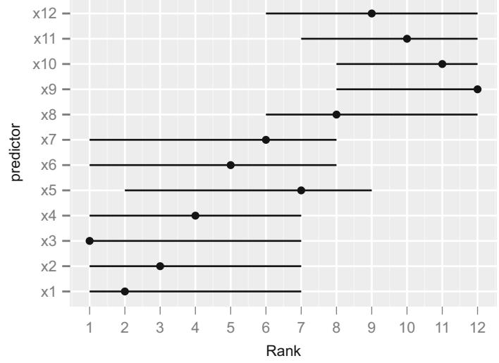
Fig. 5.3 Bootstrap percentile 0.95 confidence limits for ranks of predictors in an OLS model. Ranking is on the basis of partial χ² minus d.f. Point estimates are original ranks

the predictors. Confidence intervals are wide; for example the 0.95 confidence interval for the rank of x7 (which has a true rank of 7) is [1, 8], so we are only confident that x7 is not one of the 4 most influential predictors. The confidence intervals do include the true ranks in each case (Figure 5.3).

5.5 Simplifying the Final Model by Approximating It

5.5.1 Difficulties Using Full Models

A model that contains all prespecified terms will usually be the one that predicts the most accurately on new data. It is also a model for which confidence limits and statistical tests have the claimed properties. Often, however, this model will not be very parsimonious. The full model may require more predictors than the researchers care to collect in future samples. It also requires predicted values to be conditional on all of the predictors, which can increase the variance of the predictions.

As an example suppose that least squares has been used to fit a model containing several variables including race (with four categories). Race may be an insignificant predictor and may explain a tiny fraction of the observed variation in Y . Yet when predictions are requested, a value for race must be inserted. If the subject is of the majority race, and this race has a majority of,

say 0.75, the variance of the predicted value will not be significantly greater than the variance for a predicted value from a model that excluded race for its list of predictors. If, however, the subject is of a minority race (say “other” with a prevalence of 0.01), the predicted value will have much higher variance. One approach to this problem, that does not require development of a second model, is to ignore the subject’s race and to get a weighted average prediction. That is, we obtain predictions for each of the four races and weight these predictions by the relative frequencies of the four races.d This weighted average estimates the expected value of Y unconditional on race. It has the advantage of having exactly correct confidence limits when model assumptions are satisfied, because the correct “error term” is being used (one that deducts 3 d.f. for having ever estimated the race effect). In regression models having nonlinear link functions, this process does not yield such a simple interpretation.

When predictors are collinear, their competition results in larger P-values when predictors are (often inappropriately) tested individually. Likewise, confidence intervals for individual effects will be wide and uninterpretable (can other variables really be held constant when one is changed?).

5.5.2 Approximating the Full Model

When the full model contains several predictors that do not appreciably affect the predictions, the above process of “unconditioning” is unwieldy. In the search for a simple solution, the most commonly used procedure for making the model parsimonious is to remove variables on the basis of P-values, but this results in a variety of problems as we have seen. Our approach instead is to consider the full model fit as the “gold standard” model, especially the model from which formal inferences are made. We then proceed to approximate this full model to any desired degree of accuracy. For any approximate model we calculate the accuracy with which it approximates the best model. One goal this process accomplishes is that it provides different degrees of parsimony to different audiences, based on their needs. One investigator may be able to collect only three variables, another one seven. Each investigator will know how much she is giving up by using a subset of the predictors. In approximating the gold standard model it is very important to note that there is nothing gained in removing certain nonlinear terms; gains in parsimony come only from removing entire predictors. Another accomplishment of model approximation is that when the full model has been fitted using

^d Using the rms package described in Chapter 6, such estimates and their confidence limits can easily be obtained, using for example contrast(fit, list(age=50, disease=‘hypertension’, race=levels(race)), type=‘average’, weights=table(race)).

shrinkage (penalized estimation, Section 9.10), the approximate models will inherit the shrinkage (see Section 14.10 for an example).

Approximating complex models with simpler ones has been used to decode “black boxes” such as artificial neural networks. Recursive partitioning trees (Section 2.5) may sometimes be used in this context. One develops a regression tree to predict the predicted value Xβˆ on the basis of the unique variables in X, using R2, the average absolute prediction error, or the maximum absolute prediction error as a stopping rule, for example184. The user desiring simplicity may use the tree to obtain predicted values, using the first k nodes, with k just large enough to yield a low enough absolute error in predicting the more comprehensive prediction. Overfitting is not a problem as it is when the tree procedure is used to predict the outcome, because (1) given the predictor values the predictions are deterministic and (2) the variable being predicted is a continuous, completely observed variable. Hence the best cross-validating tree approximation will be one with one subject per node. One advantage of the tree-approximation procedure is that data collection on an individual subject whose outcome is being predicted may be abbreviated by measuring only those Xs that are used in the top nodes, until the prediction is resolved to within a tolerable error.

When principal component regression is being used, trees can also be used to approximate the components or to make them more interpretable.

Full models may also be approximated using least squares as long as the linear predictor Xβˆ is the target, and not some nonlinear transformation of it such as a logistic model probability. When the original model was fitted using unpenalized least squares, submodels fitted against Yˆ will have the same coefficients as if least squares had been used to fit the subset of predictors directly against Y . To see this, note that if X denotes the entire design matrix and T denotes a subset of the columns of X, the coefficient estimates for the full model are (X′ X)−¹X′ Y , Yˆ = X(X′ X)−¹X′ Y , estimates for a reduced model fitted against Y are (T ′ T )−¹T ′ Y , and coefficients fitted against Yˆ are (T ′ T )T ′ X(X′ X)−¹X′ Y which can be shown to equal (T ′ T )−¹T ′ Y .

When least squares is used for both the full and reduced models, the variance–covariance matrix of the coefficient estimates of the reduced model is (T ′ T )−¹σ², where the residual variance σ² is estimated using the full model. When σ² is estimated by the unbiased estimator using the d.f. from the full model, which provides the only unbiased estimate of σ², the estimated variance–covariance matrix of the reduced model will be appropriate (unlike that from stepwise variable selection) although the bootstrap may be needed to fully take into account the source of variation due to how the approximate model was selected.

So if in the least squares case the approximate model coefficients are identical to coefficients obtained upon fitting the reduced model against Y , how is model approximation any different from stepwise variable selection? There are several differences, in addition to how σ² is estimated.

1. When the full model is approximated by a backward step-down procedure against Yˆ , the stopping rule is less arbitrary. One stops deleting variables when deleting any further variable would make the approximation inadequate (e.g., the R² for predictions from the reduced model against the original Yˆ drops below 0.95).
1. Because the stopping rule is different (i.e., is not based on P-values), the approximate model will have a different number of predictors than an ordinary stepwise model.
1. If the original model used penalization, approximate models will inherit the amount of shrinkage used in the full fit.

Typically, though, if one performed ordinary backward step-down against Y using a large cutoff for α (e.g., 0.5), the approximate model would be very similar to the step-down model. The main difference would be the use of a larger estimate of σ² and smaller error d.f. than are used for the ordinary step-down approach (an estimate that pretended the final reduced model was prespecified).

When the full model was not fitted using least squares, least squares can still easily be used to approximate the full model. If the coefficient estimates from the full model are βˆ, estimates from the approximate model are matrix contrasts of βˆ, namely, Wβˆ, where W = (T ′ T )−¹T ′ X. So the variance– covariance matrix of the reduced coefficient estimates is given by

\[WW',\]

\[^{,(0,1)}\tag{5.2}\]

where V is the variance matrix for βˆ. See Section 19.5 for an example. Ambler et al.21 studied model simplification using simulation studies based on several clinical datasets, and compared it with ordinary backward stepdown variable selection and with shrinkage methods such as the lasso (see Section 4.3). They found that ordinary backwards variable selection can be competitive when there is a large fraction of truly irrelevant predictors (something that can be difficult to know in advance). Paul et al.485 found advantages to modeling the response with a complex but reliable approach, and then developing a parsimoneous model using the lasso or stepwise variable selection against Yˆ . See Section 11.7 for a case study in model approximation.

5.6 Further Reading

1 Gelman213 argues that continuous variables should be scaled by two standard deviations to make them comparable to binary predictors. However his approach assumes linearity in the predictor effect and assumes the prevalence of the binary predictor is near 0.5. John Fox [202, p. 95] points out that if two predictors are on the same scale and have the same impact (e.g., years of employment and years of education), standardizing the coefficients will make them appear to have different impacts.

2 Levine et al.401 have a compelling argument for graphing effect ratios on a logarithmic scale.
3 Hankins254 is a definitive reference on nomograms and has multi-axis examples of historical significance. According to Hankins, Maurice d’Ocagne could be called the inventor of the nomogram, starting with alignment diagrams in 1884 and declaring a new science of “nomography” in 1899. d’Ocagne was at Ecole ´ des Ponts et Chauss´ees, a French civil engineering school. Julien and Hanley328 have a nice example of adding axes to a nomogram to estimate the absolute effect of a treatment estimated using a Cox proportional hazards model. Kattan and Marasco339 have several clinical examples and explain advantages to the user of nomograms over “black box” computerized prediction.
4 Graham and Clavel231 discuss graphical and tabular ways of obtaining risk estimates. van Gorp et al.630 have a nice example of a score chart for manually obtaining estimates.
5 Larsen and Merlo375 developed a similar measure—the median odds ratio. G¨onen and Heller223 developed a c-index that like g is a function of the covariate distribution.
6 Booth and Sarkar61 have a nice analysis of the number of bootstrap resamples needed to guarantee with 0.95 confidence that a variance estimate has a sufficiently small relative error. They concentrate on the Monte Carlo simulation error, showing that small errors in variance estimates can lead to important differences in P-values. Canty et al.91 provide a number of diagnostics to check the reliability of bootstrap calculations.
7 There are many variations on the basic bootstrap for computing confidence limits.150,178 See Booth and Sarkar61 for useful information about choosing the number of resamples. They report the number of resamples necessary to not appreciably change P-values, for example. Booth and Sarkar propose a more conservative number of resamples than others use (e.g., 800 resamples) for estimating variances. Carpenter and Bithell92 have an excellent overview of bootstrap confidence intervals, with practical guidance. They also have a good discussion of the unconditional nonparametric bootstrap versus the conditional semiparametric bootstrap.
8 Altman and Royston18 have a good general discussion of what it means to validate a predictive model, including issues related to study design and consideration of uses to which the model will be put.
9 An excellent paper on external validation and generalizability is Justice et al.329. Bleeker et al.58 provide an example where internal validation is misleading when compared with a true external validation done using subjects from different centers in a different time period. Vergouwe et al.638 give good guidance about the number of events needed in sample used for external validation of binary logistic models.
10 See Picard and Berk505 for more about data-splitting.
11 In the context of variable selection where one attempts to select the set of variables with nonzero true regression coefficients in an ordinary regression model, Shao565 demonstrated that leave-out-one cross-validation selects models that are “too large.” Shao also showed that the number of observations held back for validation should often be larger than the number used to train the model. This is because in this case one is not interested in an accurate model (you fit the whole sample to do that), but an accurate estimate of prediction error is mandatory so as to know which variables to allow into the final model. Shao suggests using a cross-validation strategy in which approximately n³/⁴ observations are used in each training sample and the remaining observations are used in the test sample. A repeated balanced or Monte Carlo splitting approach is used, and accuracy estimates are averaged over 2n (for the Monte Carlo method) repeated splits.

5.6 Further Reading 123

12 Picard and Cook’s Monte Carlo cross-validation procedure506 is an improvement over ordinary cross-validation.
13 The randomization method is related to Kipnis’ “chaotization relevancy principle”348 in which one chooses between two models by measuring how far each is from a nonsense model. Tibshirani and Knight also use a randomization method for estimating the optimism in a model fit.611
14 This method used here is a slight change over that presented in [172], where Efron wrote predictive accuracy as a sum of per-observation components (such as 1 if the observation is classified correctly, 0 otherwise). Here we are writing m × the unitless summary index of predictive accuracy in the place of Efron’s sum of m per-observation accuracies [416, p. 613].
15 See [633] and [66, Section 4] for insight on the meaning of expected optimism.
16 See Copas,123 van Houwelingen and le Cessie [633, p. 1318], Verweij and van Houwelingen,640 and others631 for other methods of estimating shrinkage coefficients.
17 Efron172 developed the “.632” estimator only for the case where the index being bootstrapped is estimated on a per-observation basis. A natural generalization of this method can be derived by assuming that the accuracy evaluated on observation i that is omitted from a bootstrap sample has the same expectation as the accuracy of any other observation that would be omitted from the sample. The modified estimate of ϵ⁰ is then given by

\[ \hat{\epsilon}\_0 = \sum\_{i=1}^B w\_i T\_i,\tag{5.3} \]

where Tⁱ is the accuracy estimate derived from fitting a model on the ith bootstrap sample and evaluating it on the observations omitted from that bootstrap sample, and wⁱ are weights derived for the B bootstrap samples:

\[w\_i = \frac{1}{n} \sum\_{j=1}^{n} \frac{[\text{bootstrap sample } i \text{ emits observation } j]}{\#\text{bootstrap samples coming within } \text{observation } j}. \tag{5.4}\]

Note that ˆϵ⁰ is undefined if any observation is included in every bootstrap sample. Increasing B will avoid this problem. This modified “.632” estimator is easy to compute if one assembles the bootstrap sample assignments and computes the wⁱ before computing the accuracy indexes Ti. For large n, the wⁱ approach 1/B and so ˆϵ⁰ becomes equivalent to the accuracy computed on the observations not contained in the bootstrap sample and then averaged over the B repetitions.

18 Efron and Tibshirani179 have reduced the bias of the “.632” estimator further with only a modest increase in its variance. Simulation has, however, shown no advantage of this “.632+” method over the basic optimism bootstrap for most accuracy indexes used in logistic models.
19 van Houwelingen and le Cessie633 have several interesting developments in model validation. See Breiman66 for a discussion of the choice of X for which to validate predictions. Steyerberg et al.587 present simulations showing the number of bootstrap samples needed to obtain stable estimates of optimism of various accuracy measures. They demonstrate that bootstrap estimates of optimism are nearly unbiased when compared with simulated external estimates. They also discuss problems with precision of estimates of accuracy, especially when using external validation on small samples.
20 Blettner and Sauerbrei also demonstrate the variability caused by data-driven analytic decisions.59 Chatfield100 has more results on the effects of using the data to select the model.

5.7 Problem

Perform a simulation study to understand the performance of various internal validation methods for binary logistic models. Modify the R code below in at least two meaningful ways with regard to covariate distribution or number, sample size, true regression coefficients, number of resamples, or number of times certain strategies are averaged. Interpret your findings and give recommendations for best practice for the type of configuration you studied. The R code from this assignment may be downloaded from the RMS course wiki page.

For each of 200 simulations, the code below generates a training sample of 200 observations with p predictors (p = 15 or 30) and a binary response. The predictors are independently U(−0.5, 0.5). The response is sampled so as to follow a logistic model where the intercept is zero and all regression coefficients equal 0.5. The “gold standard” is the predictive ability of the fitted model on a test sample containing 50,000 observations generated from the same population model. For each of the 200 simulations, several validation methods are employed to estimate how the training sample model predicts responses in the 50,000 observations. These validation methods involve fitting 40 or 200 models in resamples.

g-fold cross-validation is done using the command validate(f, method= ‘cross’, B=g) using the rms package. This was repeated and averaged using an extra loop, shown below.

For bootstrap methods, validate(f, method=‘boot’ or ‘.632’, B=40 or B=200) was used. method=‘.632’ does Efron’s “.632”method179, labeled 632a in the output. An ad-hoc modification of the .632 method, 632b was also done. Here a “bias-corrected”index of accuracy is simply the index evaluated in the observation omitted from the bootstrap resample. The “gold standard” external validations were obtained from the val.prob function in the rms package. The following indexes of predictive accuracy are used:

Dxy: Somers’ rank correlation between predicted probability that Y = 1 vs. the binary Y values. This equals 2(C − 0.5) where C is the “ROC Area” or concordance probability.
D: Discrimination index likelihood ratio χ² divided by the sample size
U: Unreliability index unitless index of how far the logit calibration curve intercept and slope are from (0, 1)
Q: Logarithmic accuracy score a scaled version of the log-likelihood achieved by the predictive model

Intercept: Calibration intercept on logit scale

Slope: Calibration slope (slope of predicted log odds vs. true log odds)

Accuracy of the various resampling procedures may be estimated by computing the mean absolute errors and the root mean squared errors of estimates (e.g., of Dxy from the bootstrap on the 200 observations) against the “gold standard” (e.g., Dxy for the fitted 200-observation model achieved in the 50,000 observations).

require (rms)
set.seed (1) # so can reproduce results
n ← 200 # Size of training sample
reps ← 200 # Simulations
npop ← 50000 # Size of validation gold standard sample
methods ← c( ' Boot 40 ' , ' Boot 200 ' , ' 632a 40 ' , ' 632a 200 ' ,
              ' 632b 40 ' , ' 632b 200 ' , ' 10-fold x 4 ' , ' 4-fold x 10 ' ,
              ' 10-fold x 20 ' , ' 4-fold x 50 ' )
R ← expand.grid (sim = 1:reps ,
                 p = c(15,30),
                 method = methods)
R$Dxy ← R$Intercept ← R$Slope ← R$D ← R$U ← R$Q ←
  R$repmeth ← R$B ← NA
R$n ← n
## Function to do r overall reps of B resamples , averaging to
## get estimates similar to as if r*B resamples were done
val ← function (fit , method , B, r) {
  contains ← function (m) length(grep(m, method)) > 0
  meth ← if(contains ( ' Boot ' )) ' boot ' else
          if(contains ( ' fold ' )) ' crossvalidation ' else
          if(contains ( ' 632 ' )) ' .632 '
  z ← 0
  for(i in 1:r) z ← z + validate (fit , method=meth , B=B)[
          c("Dxy","Intercept ","Slope","D","U","Q"),
          ' index.corrected ' ]
  z/r
}

for(p in c(15, 30)) {
  ## For each p create the true betas , the design matrix ,
  ## and realizations of binary y in the gold standard
  ## large sample
  Beta ← rep(.5 , p) # True betas
  X ← matrix (runif (npop*p), nrow=npop) - 0.5
  LX ← matxv (X, Beta)
  Y ← ifelse (runif (npop) ≤ plogis (LX), 1, 0)
  ## For each simulation create the data matrix and
  ## realizations of y
  for(j in 1:reps) {
    ## Make training sample
    x ← matrix (runif (n*p), nrow=n) - 0.5
    L ← matxv (x, Beta)
    y ← ifelse (runif (n) ≤ plogis (L), 1, 0)
    f ← lrm(y ∼ x, x=TRUE , y= TRUE)
    beta ← f$coef
    forecast ← matxv(X, beta)
    ## Validate in population

v ← val.prob( logit =forecast , y=Y, pl=FALSE )[
                      c("Dxy","Intercept"," Slope ","D","U","Q")]
    for(method in methods) {
      repmeth ← 1
      if(method %in% c( ' Boot 40 ' , ' 632a 40 ' , ' 632b 40 ' ))
        B ← 40
      if(method %in% c( ' Boot 200 ' , ' 632a 200 ' , ' 632b 200 ' ))
        B ← 200
      if(method == ' 10-fold x 4 ' ) {
        B ← 10
         repmeth ← 4
      }
      if(method == ' 4-fold x 10 ' ) {
        B ← 4
         repmeth ← 10
      }
      if(method == ' 10-fold x 20 ' ) {
        B ← 10
         repmeth ← 20
      }
      if(method == ' 4-fold x 50 ' ) {
        B ← 4
         repmeth ← 50
      }
      z ← val(f, method , B, repmeth)
      k ← which (R$sim == j & R$p == p & R$method == method )
      if(length (k) != 1) stop( ' program logic error ' )
      R[k, names (z)] ← z-v
      R[k, c( ' B ' , ' repmeth ' )] ← c(B=B, repmeth=repmeth)
    } # end over methods
  } # end over reps
} # end over p

Results are best summarized in a multi-way dot chart. Bootstrap nonparametric percentile 0.95 confidence limits are included.

statnames ← names (R )[6:11]
w ← reshape(R, direction= ' long ' , varying= list( statnames),
              v.names= ' x ' , timevar= ' stat ' , times = statnames)
w$p ← paste ( ' p ' , w$p, sep= ' = ' )
require(lattice)
s ← with(w, summarize(abs(x), llist(p, method , stat),
                         smean.cl.boot ,stat.name= ' mae ' ))
Dotplot( method ∼ Cbind (mae , Lower , Upper ) | stat*p, data=s,
         xlab= ' Mean |error| ' )
s ← with(w, summarize(x∧2, llist(p, method , stat),
                         smean.cl.boot , stat.name= ' mse ' ))
Dotplot( method ∼ Cbind (sqrt(mse), sqrt(Lower ), sqrt(Upper )) |
         stat*p, data=s,
         xlab= expression( sqrt(MSE)))

Chapter 6 R Software

The methods described in this book are useful in any regression model that involves a linear combination of regression parameters. The software that is described below is useful in the same situations. Functions in R520 allow interaction spline functions as well as a wide variety of predictor parameterizations for any regression function, and facilitate model validation by resampling. ¹

R is the most comprehensive tool for general regression models for the following reasons.

1. It is very easy to write R functions for new models, so R has implemented a wide variety of modern regression models.
1. Designs can be generated for any model. There is no need to find out whether the particular modeling function handles what SAS calls “class” variables—dummy variables are generated automatically when an R category, factor, ordered, or character variable is analyzed.
1. A single R object can contain all information needed to test hypotheses and to obtain predicted values for new data.
1. R has superior graphics.
1. Classes in R make possible the use of generic function names (e.g., predict, summary, anova) to examine fits from a large set of specific model–fitting functions.

R44, 601, 635 is a high-level object-oriented language for statistical analysis with over six thousand packages and tens of thousands of functions available. The R system318, 520 is the basis for R software used in this text, centered around the Regression Modeling Strategies (rms) package261. See the Appendix and the Web site for more information about software implementations.

^© Springer International Publishing Switzerland 2015 F.E. Harrell, Jr., Regression Modeling Strategies, Springer Series in Statistics, DOI 10.1007/978-3-319-19425-7 6

6.1 The R Modeling Language

R has a battery of functions that make up a statistical modeling language.96 2 At the heart of the modeling functions is an R formula of the form

response ∼ terms

The terms represent additive components of a general linear model. Although variables and functions of variables make up the terms, the formula refers to additive combinations; for example, when terms is age + blood.pressure, it refers to β¹ × age + β² × blood.pressure. Some examples of formulas are below.

y ∼ age + sex # age + sex main effects
y ∼ age + sex + age:sex # add second-order interaction
y ∼ age*sex # second-order interaction +
                        # all main effects
y ∼ (age + sex + pressure)∧2
                # age+sex+pressure+age:sex+age:pressure...
y ∼ (age + sex + pressure)∧2 - sex:pressure
                      # all main effects and all 2nd order
                      # interactions except sex:pressure
y ∼ (age + race)*sex # age+race+sex+age:sex+race:sex
y ∼ treatment*(age* race + age*sex)
                        # no interact. with race ,sex
sqrt(y) ∼ sex*sqrt(age) + race
# functions, with dummy variables generated if
# race is an R factor (classification ) variable
y ∼ sex + poly (age ,2) # poly makes orthogonal polynomials
race.sex ← interaction (race ,sex)
y ∼ age + race.sex # if desire dummy variables for all
                    # combinations of the factors

The formula for a regression model is given to a modeling function; for example,

lrm(y ∼ rcs(x,4))

is read “use a logistic regression model to model y as a function of x, representing x by a restricted cubic spline with four default knots.”a You can use the R function update to refit a model with changes to the model terms or the data used to fit it:

f ← lrm(y ∼ rcs(x,4) + x2 + x3)
f2 ← update (f, subset =sex=="male")
f3 ← update (f, .∼.-x2) # remove x2 from model
f4 ← update (f, .∼. + rcs(x5 ,5)) # add rcs(x5 ,5) to model
f5 ← update (f, y2 ∼ . ) # same terms , new response var.

^a lrm and rcs are in the rms package.

6.2 User-Contributed Functions

In addition to the many functions that are packaged with R, a wide variety of user-contributed functions is available on the Internet (see the Appendix or Web site for addresses). Two packages of functions used extensively in this text are Hmisc20 and rms written by the author. The Hmisc package contains miscellaneous functions such as varclus, spearman2, transcan, hoeffd, rcspline.eval, impute, cut2, describe, sas.get, latex, and several power and sample size calculation functions. The varclus function uses the R hclust hierarchical clustering function to do variable clustering, and the R plclust function to draw dendrograms depicting the clusters. varclus offers a choice of three similarity measures (Pearson r2, Spearman ρ2, and Hoeffding D) and uses pairwise deletion of missing values. varclus automatically generates a series of dummy variables for categorical factors. The Hmisc hoeffd function computes a matrix of Hoeffding Ds for a series of variables. The spearman2 function will do Wilcoxon, Spearman, and Kruskal–Wallis tests and generalizes Spearman’s ρ to detect non-monotonic relationships.

Hmisc’s transcan function (see Section 4.7) performs a similar function to PROC PRINQUAL in SAS—it uses restricted splines, dummy variables, and canonical variates to transform each of a series of variables while imputing missing values. An option to shrink regression coefficients for the imputation models avoids overfitting for small samples or a large number of predictors. transcan can also do multiple imputation and adjust variance–covariance matrices for imputation. See Chapter 8 for an example of using these functions for data reduction.

See the Web site for a list of R functions for correspondence analysis, principal component analysis, and missing data imputation available from other users. Venables and Ripley [635, Chapter 11] provide a nice description of the multivariate methods that are available in R, and they provide several new multivariate analysis functions.

A basic function in Hmisc is the rcspline.eval function, which creates a design matrix for a restricted (natural) cubic spline using the truncated power basis. Knot locations are optionally estimated using methods described in Section 2.4.6, and two types of normalizations to reduce numerical problems are supported. You can optionally obtain the design matrix for the antiderivative of the spline function. The rcspline.restate function computes the coefficients (after un-normalizing if needed) that translate the restricted cubic spline function to unrestricted form (Equation 2.27). rcspline.restate also outputs LATEX and R representations of spline functions in simplified form.

6.3 The rms Package

A package of R functions called rms contains several functions that extend R to make the analyses described in this book easy to do. A central function in rms is datadist, which computes statistical summaries of predictors to automate estimation and plotting of effects. datadist exists as a separate function so that the candidate predictors may be summarized once, thus saving time when fitting several models using subsets or different transformations of predictors. If datadist is called before model fitting, the distributional summaries are stored with the fit so that the fit is self-contained with respect to later estimation. Alternatively, datadist may be called after the fit to create temporary summaries to use as plot ranges and effect intervals, or these ranges may be specified explicitly to Predict and summary (see below), without ever calling datadist. The input to datadist may be a data frame, a list of individual predictors, or a combination of the two.

The characteristics saved by datadist include the overall range and certain quantiles for continuous variables, and the distinct values for discrete variables (i.e., R factor variables or variables with 10 or fewer unique values). The quantiles and set of distinct values facilitate estimation and plotting, as described later. When a function of a predictor is used (e.g., pol(pmin(x,50),2)), the limits saved apply to the innermost variable (here, x). When a plot is requested for how x relates to the response, the plot will have x on the x-axis, not pmin(x,50). The way that defaults are computed can be controlled by the q.effect and q.display parameters to datadist. By default, continuous variables are plotted with ranges determined by the tenth smallest and tenth largest values occurring in the data (if n < 200, the 0.05 and 0.95 quantiles are used). The default range for estimating effects such as odds and hazard ratios is the lower and upper quartiles. When a predictor is adjusted to a constant so that the effects of changes in other predictors can be studied, the default constant used is the median for continuous predictors and the most frequent category for factor variables. The R system option datadist is used to point to the result returned by the datadist function. See the help files for datadist for more information.

rms fitting functions save detailed information for later prediction, plotting, and testing. rms also allows for special restricted interactions and sets the default method of generating contrasts for categorical variables to “contr. treatment”, the traditional dummy-variable approach.

rms has a special operator %ia% in the terms of a formula that allows for restricted interactions. For example, one may specify a model that contains sex and a five-knot linear spline for age, but restrict the age × sex interaction to be linear in age. To be able to connect this incomplete interaction with the main effects for later hypothesis testing and estimation, the following formula would be given:

y ∼ sex + lsp(age ,c(20 ,30 ,40 ,50 ,60)) +
    sex %ia% lsp(age ,c(20 ,30 ,40 ,50 ,60))

Function	Purpose	Related R
		Functions
ols	Ordinary least squares linear model	lm
lrm	Binary and ordinal logistic regression model	glm
	Has options for penalized MLE
orm	Ordinal semi-parametric regression model with	polr,lrm
	several link functions
psm	Accelerated failure time parametric survival	survreg
	models
cph	Cox proportional hazards regression	coxph
bj	Buckley–James censored least squares model	survreg,lm
Glm	General linear models	glm
Gls	Generalized least squares	gls
Rq	Quantile regression	rq

Table 6.1 rms Fitting Functions

The following expression would restrict the age × cholesterol interaction to be of the form AF(B) + BG(A) by removing doubly nonlinear terms.

y ∼ lsp(age ,30) + rcs(cholesterol ,4) +
    lsp(age ,30) %ia% rcs(cholesterol ,4)

rms has special fitting functions that facilitate many of the procedures described in this book, shown in Table 6.1.

Glm is a slight modification of the built-in R glm function so that rms methods can be run on the resulting fit object. glm fits general linear models under a wide variety of distributions of Y . Gls is a modification of the gls function from the nlme package of Pinheiro and Bates509, for repeated measures (longitudinal) and spatially correlated data. The Rq function is a modification of the quantreg package’s rq function356, 357. Functions related to survival analysis make heavy use of Therneau’s survival package482.

You may want to specify to the fitting functions an option for how missing values (NAs) are handled. The method for handling missing data in R is to specify an na.action function. Some possible na.actions are given in Table 6.2. The default na.action is na.delete when you use rms’s fitting functions. An easy way to specify a new default na.action is, for example,

options(na.action="na.omit")# don ' t report frequency of NAs

before using a fitting function. If you use na.delete you can also use the system option na.detail.response that makes model fits store information about Y stratified by whether each X is missing. The default descriptive statistics for Y are the sample size and mean. For a survival time response object the sample size and proportion of events are used. Other summary functions can be specified using the na.fun.response option.

Function Name	Method Used
na.fail	Stop with error message if any missing
	values present
na.omit	Function to remove observations with
	any predictors or responses missing
na.delete	Modified version of na.omit to also
	report on frequency of NAs for each
	variable

Table 6.2 Some na.actions Used in rms

options(na.action="na.delete", na.detail.response =TRUE ,
        na.fun.response ="mystats")
# Just use na.fun.response ="quantile" if don ' t care about n
mystats ← function(y) {
  z ← quantile(y, na.rm=T)
  n ← sum(!is.na (y))
  c(N=n, z) # elements named N, 0%, 25%, etc.
}

When R deletes missing values during the model–fitting procedure, residuals, fitted values, and other quantities stored with the fit will not correspond rowfor-row with observations in the original data frame (which retained NAs). This is problematic when, for example, age in the dataset is plotted against the residual from the fitted model. Fortunately, for many na.actions including na.delete and a modified version of na.omit, a class of R functions called naresid written by Therneau works behind the scenes to put NAs back into residuals, predicted values, and other quantities when the predict or residuals functions (see below) are used. Thus for some of the na.actions, predicted values and residuals will automatically be arranged to match the original data.

Any R function can be used in the terms for formulas given to the fitting function, but if the function represents a transformation that has datadependent parameters (such as the standard R functions poly or ns), R will not in general be able to compute predicted values correctly for new observations. For example, the function ns that automatically selects knots for a B-spline fit will not be conducive to obtaining predicted values if the knots are kept “secret.” For this reason, a set of functions that keep track of transformation parameters, exists in rms for use with the functions highlighted in this book. These are shown in Table 6.3. Of these functions, asis, catg, scored, and matrx are almost always called implicitly and are not mentioned by the user. catg is usually called explicitly when the variable is a numeric variable to be used as a polytomous factor, and it has not been converted to an R categorical variable using the factor function.

Function	Purpose	Related R
		Functions
asis	No post-transformation (seldom used explicitly)	I
rcs	Restricted cubic spline	ns
pol	Polynomial using standard notation	poly
lsp	Linear spline
catg	Categorical predictor (seldom)	factor
scored	Ordinal categorical variables	ordered
matrx	Keep variables as group for anova and fastbw	matrix
strat	Nonmodeled stratification factors	strata
	(used for cph only)

Table 6.3 rms Transformation Functions

These functions can be used with any function of a predictor. For example, to obtain a four-knot cubic spline expansion of the cube root of x, specify rcs(x∧(1/3),4).

When the transformation functions are called, they are usually given one or two arguments, such as rcs(x,5). The first argument is the predictor variable or some function of it. The second argument is an optional vector of parameters describing a transformation, for example location or number of knots. Other arguments may be provided.

The Hmisc package’s cut2 function is sometimes used to create a categorical variable from a continuous variable x. You can specify the actual interval endpoints (cuts), the number of observations to have in each interval on the average (m), or the number of quantile groups (g). Use, for example, cuts=c(0,1,2) to cut into the intervals [0, 1), [1, 2].

A key concept in fitting models in R is that the fitting function returns an object that is an R list. This object contains basic information about the fit (e.g., regression coefficient estimates and covariance matrix, model χ²) as well as information about how each parameter of the model relates to each factor in the model. Components of the fit object are addressed by, for example, fit$coef, fit$var, fit$loglik. rms causes the following information to also be retained in the fit object: the limits for plotting and estimating effects for each factor (if options(datadist=“name”) was in effect), the label for each factor, and a vector of values indicating which parameters associated with a factor are nonlinear (if any). Thus the “fit object” contains all the information needed to get predicted values, plots, odds or hazard ratios, and hypothesis tests, and to do “smart” variable selection that keeps parameters together when they are all associated with the same predictor.

R uses the notion of the class of an object. The object-oriented class idea allows one to write a few generic functions that decide which specific functions to call based on the class of the object passed to the generic function. An example is the function for printing the main results of a logistic model. The lrm function returns a fit object of class “lrm”. If you specify the R command print(fit) (or just fit if using R interactively—this invokes print), the print function invokes the print.lrm function to do the actual printing specific to logistic models. To find out which particular methods are implemented for a given generic function, type methods(generic.name).

Generic functions that are used in this book include those in Table 6.4.

Function Purpose Related Functions print Print parameters and statistics of fit coef Fitted regression coefficients formula Formula used in the fit specs Detailed specifications of fit vcov Fetch covariance matrix logLik Fetch maximized log-likelihood AIC Fetch AIC lrtest Likelihood ratio test for two nested models univarLR Compute all univariable LR χ² robcov Robust covariance matrix estimates bootcov Bootstrap covariance matrix estimates and bootstrap distributions of estimates pentrace Find optimum penalty factors by tracing effective AIC for a grid of penalties effective.df Print effective d.f. for each type of variable in model, for penalized fit or pentrace result summary Summary of effects of predictors plot.summary Plot continuously shaded confidence bars for results of summary anova Wald tests of most meaningful hypotheses plot.anova Graphical depiction of anova contrast General contrasts, C.L., tests Predict Predicted values and confidence limits easily varying a subset of predictors and leaving the rest set at default values plot.Predict Plot the result of Predict using lattice ggplot Plot the result of Predict using ggplot2 bplot 3-dimensional plot when Predict varied two continuous predictors over a fine grid gendata Easily generate predictor combinations predict Obtain predicted values or design matrix fastbw Fast backward step-down variable selection step residuals (or resid) Residuals, influence stats from fit sensuc Sensitivity analysis for unmeasured confounder which.influence Which observations are overly influential residuals latex LATEX representation of fitted model Function continued on next page

Table 6.4 rms Package and R Generic Functions

		continued from previous page
Function	Purpose	Related Functions
Function	R function analytic representation of Xβˆ	latex
	from a fitted regression model
Hazard	R function analytic representation of a fitted
	hazard function (for psm)
Survival	R function analytic representation of fitted
	survival function (for psm, cph)
ExProb	R function analytic representation of
	exceedance probabilities for orm
Quantile	R function analytic representation of fitted
	function for quantiles of survival time
	(for psm, cph)
Mean	R function analytic representation of fitted
	function for mean survival time or for ordinal logistic
nomogram	Draws a nomogram for the fitted model	latex, plot
survest	Estimate survival probabilities (psm, cph)	survfit
survplot	Plot survival curves (psm, cph)	plot.survfit
validate	Validate indexes of model fit using resampling
	calibrate Estimate calibration curve using resampling	val.prob
vif	Variance inflation factors for fitted model
naresid	Bring elements corresponding to missing data
	back into predictions and residuals
naprint	Print summary of missing values
impute	Impute missing values	transcan

The first argument of the majority of functions is the object returned from the model fitting function. When used with ols, lrm, orm, psm, cph, Glm, Gls, Rq, bj, these functions do the following. specs prints the design specifications, for example, number of parameters for each factor, levels of categorical factors, knot locations in splines, and so on. vcov returns the variance-covariance matrix for the model. logLik retrieves the maximized log-likelihood, whereas AIC computes the Akaike Information Criterion for the model on the minus twice log-likelihood scale (with an option to compute it on the χ² scale if you specify type=‘chisq’). lrtest, when given two fit objects from nested models, computes the likelihood ratio test for the extra variables. univarLR computes all univariable likelihood ratio χ² statistics, one predictor at a time.

The robcov function computes the Huber robust covariance matrix estimate. bootcov uses the bootstrap to estimate the covariance matrix of parameter estimates. Both robcov and bootcov assume that the design matrix and response variable were stored with the fit. They have options to adjust for cluster sampling. Both replace the original variance–covariance matrix with robust estimates and return a new fit object that can be passed to any of the other functions. In that way, robust Wald tests, variable selection, confidence limits, and many other quantities may be computed automatically. The functions do save the old covariance estimates in component orig.var of the new fit object. bootcov also optionally returns the matrix of parameter estimates over the bootstrap simulations. These estimates can be used to derive bootstrap confidence intervals that don’t assume normality or symmetry. Associated with bootcov are plotting functions for drawing histogram and smooth density estimates for bootstrap distributions. bootcov also has a feature for deriving approximate nonparametric simultaneous confidence sets. For example, the function can get a simultaneous 0.90 confidence region for the regression effect of age over its entire range.

The pentrace function assists in selection of penalty factors for fitting regression models using penalized maximum likelihood estimation (see Section 9.10). Different types of model terms can be penalized by different amounts. For example, one can penalize interaction terms more than main effects. The effective.df function prints details about the effective degrees of freedom devoted to each type of model term in a penalized fit.

summary prints a summary of the effects of each factor. When summary is used to estimate effects (e.g., odds or hazard ratios) for continuous variables, it allows the levels of interacting factors to be easily set, as well as allowing the user to choose the interval for the effect. This method of estimating effects allows for nonlinearity in the predictor. By default, interquartile range effects (differences in Xβˆ, odds ratios, hazards ratios, etc.) are printed for continuous factors, and all comparisons with the reference level are made for categorical factors. See the example at the end of the summary documentation for a method of quickly computing pairwise treatment effects and confidence intervals for a large series of values of factors that interact with the treatment variable. Saying plot(summary(fit)) will depict the effects graphically, with bars for a list of confidence levels.

The anova function automatically tests most meaningful hypotheses in a design. For example, suppose that age and cholesterol are predictors, and that a general interaction is modeled using a restricted spline surface. anova prints Wald statistics for testing linearity of age, linearity of cholesterol, age effect (age + age × cholesterol interaction), cholesterol effect (cholesterol + age × cholesterol interaction), linearity of the age × cholesterol interaction (i.e., adequacy of the simple age × cholesterol 1 d.f. product), linearity of the interaction in age alone, and linearity of the interaction in cholesterol alone. Joint tests of all interaction terms in the model and all nonlinear terms in the model are also performed. The plot.anova function draws a dot chart showing the relative contribution (χ², χ² minus d.f., AIC, partial R², P-value, etc.) of each factor in the model.

The contrast function is used to obtain general contrasts and corresponding confidence limits and test statistics. This is most useful for testing effects in the presence of interactions (e.g., type II and type III contrasts). See the help file for contrast for several examples of how to obtain joint tests of multiple contrasts (see Section 9.3.2) as well as double differences (interaction contrasts).

The predict function is used to obtain a variety of values or predicted values from either the data used to fit the model or a new dataset. The Predict function is easier to use for most purposes, and has a special plot method. The gendata function makes it easy to obtain a data frame containing predictor combinations for obtaining selected predicted values.

The fastbw function performs a slightly inefficient but numerically stable version of fast backward elimination on factors, using a method based on Lawless and Singhal.385 This method uses the fitted complete model and computes approximate Wald statistics by computing conditional (restricted) maximum likelihood estimates assuming multivariate normality of estimates. It can be used in simulations since it returns indexes of factors retained and dropped:

fit ← ols(y ∼ x1*x2*x3)
# run , and print results:
fastbw (fit , optional_arguments )
# typically used in simulations:
z ← fastbw (fit , optional_args )
# least squares fit of reduced model:
lm.fit (X[,z$ parms.kept], Y)

fastbw deletes factors, not columns of the design matrix. Factors requiring multiple d.f. will be retained or dropped as a group. The function prints the deletion statistics for each variable in turn, and prints approximate parameter estimates for the model after deleting variables. The approximation is better when the number of factors deleted is not large. For ols, the approximation is exact.

The which.influence function creates a list with a component for each factor in the model. The names of the components are the factor names. Each component contains the observation identifiers of all observations that are “overly influential” with respect to that factor, meaning that ^|dfbetas^| > u for at least one βⁱ associated with that factor, for a given u. The default u is .2. You must have specified x=TRUE, y=TRUE in the fitting function to use which.influence. The first argument is the fit object, and the second argument is the cutoff u.

The following R program will print the set of predictor values that were very influential for each factor. It assumes that the data frame containing the data used in the fit is called df.

f ← lrm(y ∼ x1 + x2 + ... , data =df , x=TRUE , y= TRUE)
w ← which.influence (f, .4)
nam ← names (w)
for(i in 1:length (nam)) {
   cat("Influential observations for effect of",
       nam[i],"\n")
   print (df[w[[i]],])
}

The latex function is a generic function available in the Hmisc package. It invokes a specific latex function for most of the fit objects created by rms to create a LATEX algebraic representation of the fitted model for inclusion in a report or viewing on the screen. This representation documents all parameters in the model and the functional form being assumed for Y , and is especially useful for getting a simplified version of restricted cubic spline functions. On the other hand, the print method with optional argument latex=TRUE is used to output LATEX code representing the model results in tabular form to the console. This is intended for use with knitr677 or Sweave399.

The Function function composes an R function that you can use to evaluate Xβˆ analytically from a fitted regression model. The documentation for Function also shows how to use a subsidiary function sascode that will (almost) translate such an R function into SAS code for evaluating predicted values in new subjects. Neither Function nor latex handles third-order interactions.

The nomogram function draws a partial nomogram for obtaining predictions from the fitted model manually. It constructs different scales when interactions (up to third-order) are present. The constructed nomogram is not complete, in that point scores are obtained for each predictor and the user must add the point scores manually before reading predicted values on the final axis of the nomogram. The constructed nomogram is useful for interpreting the model fit, especially for non-monotonically transformed predictors (their scales wrap around an axis automatically).

The vif function computes variance inflation factors from the covariance matrix of a fitted model, using [147, 654].

The impute function is another generic function. It does simple imputation by default. It can also work with the transcan function to multiply or singly impute missing values using a flexible additive model.

As an example of using many of the functions, suppose that a categorical variable treat has values “a”, “b”, and “c”, an ordinal variable num.diseases has values 0,1,2,3,4, and that there are two continuous variables, age and cholesterol. age is fitted with a restricted cubic spline, while cholesterol is transformed using the transformation log(cholesterol+10). Cholesterol is missing on three subjects, and we impute these using the overall median cholesterol. We wish to allow for interaction between treat and cholesterol. The following R program will fit a logistic model, test all effects in the design, estimate effects, and plot estimated transformations. The fit for num.diseases really considers the variable to be a five-level categorical variable. The only difference is that a 3 d.f. test of linearity is done to assess whether the variable can be remodeled “asis”. Here we also show statements to attach the rms package and store predictor characteristics from datadist.

require(rms) # make new functions available
ddist ← datadist( cholesterol , treat , num.diseases , age)
# Could have used ddist ← datadist(data.frame.name )
options(datadist=" ddist") # defines data dist. to rms
cholesterol ← impute ( cholesterol)
fit ← lrm(y ∼ treat + scored ( num.diseases ) + rcs(age) +
               log(cholesterol +10) +
               treat:log( cholesterol +10))
describe(y ∼ treat + scored ( num.diseases ) + rcs(age))
# or use describe(formula(fit)) for all variables used in
# fit. describe function (in Hmisc) gets simple statistics
# on variables
# fit ← robcov(fit)# Would make all statistics that follow

# use a robust covariance matrix
                    # would need x=TRUE , y= TRUE in lrm()
specs (fit) # Describe the design characteristics
anova (fit)
anova (fit , treat , cholesterol) # Test these 2 by themselves
plot(anova (fit)) # Summarize anova graphically
summary(fit) # Est. effects; default ranges
plot( summary(fit)) # Graphical display of effects with C.I.
# Specific reference cell and adjustment value:
summary(fit , treat ="b", age=60)
# Estimate effect of increasing age: 50->70
summary(fit , age=c(50 ,70))
# Increase age 50->70, adjust to 60 when estimating
# effects of other factors:
summary(fit , age=c(50 ,60 ,70))
# If had not defined datadist , would have to define
# ranges for all variables
# Estimate and test treatment (b-a) effect averaged
# over 3 cholesterols :
contrast (fit , list(treat= ' b ' , cholesterol =c (150,200 ,250)) ,
              list(treat= ' a ' , cholesterol =c (150,200 ,250)) ,
         type= ' average ' )
p ← Predict(fit , age=seq(20,80, length =100), treat ,
             conf.int= FALSE)
plot(p) # Plot relationship between age and
# or ggplot(p) # log odds , separate curve for each
                     # treat , no C.I.
plot(p, ∼ age | treat) # Same but 2 panels
ggplot (p, groups =FALSE)
bplot ( Predict(fit , age , cholesterol , np=50))
                     # 3-dimensional perspective plot for
                     # age , cholesterol , and log odds
                     # using default ranges for both
# Plot estimated probabilities instead of log odds:
plot( Predict(fit , num.diseases ,
             fun=function (x) 1/(1+ exp(-x)),
             conf.int=.9), ylab="Prob")
# Again , if no datadist were defined , would have to tell
# plot all limits
logit ← predict(fit , expand.grid ( treat ="b", num.dis =1:3,
                  age=c(20,40,60),
                  cholesterol =seq (100,300, length =10)))
# Could obtain list of predictor settings interactively
logit ← predict(fit , gendata(fit , nobs =12))
# An easier approach is
# Predict(fit , treat = ' b ' , num.dis =1:3,...)
# Since age doesn ' t interact with anything , we can quickly
# and interactively try various transformations of age ,
# taking the spline function of age as the gold standard.
# We are seeking a linearizing transformation.

ag ← 10:80
logit ← predict(fit , expand.grid ( treat ="a", num.dis =0,
                 age=ag ,
                 cholesterol= median ( cholesterol )),
                 type="terms ")[,"age"]
# Note: if age interacted with anything , this would be the
# age ` main effect ' ignoring interaction terms
# Could also use logit ← Predict(f, age=ag , ...)$yhat ,
# which allows evaluation of the shape for any level of
# interacting factors. When age does not interact with
# anything , the result from predict(f, ... , type =" terms")
# would equal the result from Predict if all other terms
# were ignored
# Could also specify:
# logit ← predict(fit ,
# gendata(fit , age=ag , cholesterol =...))
# Unmentioned variables are set to reference values
plot(ag∧.5 , logit ) # try square root vs. spline transform.
plot(ag∧1.5 , logit ) # try 1.5 power
# Pretty printing of table of estimates and
# summary statistics:
print (fit , latex =TRUE) # print LATEX code to console
latex (fit) # invokes latex.lrm, creates fit.tex
# Draw a nomogram for the model fit
plot( nomogram(fit))
# Compose R function to evaluate linear predictors
# analytically
g ← Function(fit)
g(treat= ' b ' , cholesterol =260, age =50)
# Letting num.diseases default to reference value

To examine interactions in a simpler way, you may want to group age into tertiles:

age.tertile ← cut2 (age , g=3)
# For auto ranges later , specify age.tertile to datadist
fit ← lrm(y ∼ age.tertile * rcs(cholesterol ))

Example output from these functions is shown in Chapter 10 and later chapters.

Note that type=“terms” in predict scores each factor in a model with its fitted transformation. This may be used to compute, for example, rank correlation between the response and each transformed factor, pretending it has 1 d.f.

When regression is done on principal components, one may use an ordinary linear model to decode “internal” regression coefficients for helping to understand the final model. Here is an example.

require(rms)
dd ← datadist(my.data)
options(datadist= ' dd ' )
pcfit ← princomp(∼ pain.symptom1 + pain.symptom2 + sign1 +
                    sign2 + sign3 + smoking)
pc2 ← pcfit $scores [,1:2] # first 2 PCs as matrix
logistic.fit ← lrm(death ∼ rcs(age ,4) + pc2)
predicted.logit ← predict(logistic.fit )
linear.mod ← ols(predicted.logit ∼ rcs(age ,4) +
                       pain.symptom1 + pain.symptom2 +
                       sign1 + sign2 + sign3 + smoking)
# This model will have R-squared =1
nom ← nomogram( linear.mod , fun= function (x)1/(1+ exp(-x)),
         funlabel="Probability of Death")
# can use fun=plogis
plot(nom)
# 7 Axes showing effects of all predictors , plus a reading
# axis converting to predicted probability scale

In addition to many of the add-on functions described above, there are several other R functions that validate models. The first, predab.resample, is a general-purpose function that is used by functions for specific models described later. predab.resample computes estimates of optimism and biascorrected estimates of a vector of indexes of predictive accuracy, for a model with a specified design matrix, with or without fast backward step-down of predictors. If bw=TRUE, predab.resample prints a matrix of asterisks showing which factors were selected at each repetition, along with a frequency distribution of the number of factors retained across resamples. The function has an optional parameter that may be specified to force the bootstrap algorithm to do sampling with replacement from clusters rather than from original records, which is useful when each subject has multiple records in the dataset. It also has a parameter that can be used to validate predictions in a subset of the records even though models are refit using all records.

The generic function validate invokes predab.resample with model-specific fits and measures of accuracy. The function calibrate invokes predab.resample to estimate bias-corrected model calibration and to plot the calibration curve. Model calibration is estimated at a sequence of predicted values.

6.4 Other Functions

For principal component analysis, R has the princomp and prcomp functions. Canonical correlations and canonical variates can be easily computed using the cancor function. There are many other R functions for examining associations and for fitting models. The supsmu function implements Friedman’s “super smoother.”207 The lowess function implements Cleveland’s twodimensional smoother.111 The glm function will fit general linear models under a wide variety of distributions of Y . There are functions to fit Hastie and Tibshirani’s275 generalized additive model for a variety of distributions. More is said about parametric and nonparametric additive multiple regression functions in Chapter 16. The loess function fits a multidimensional scatterplot smoother (the local regression model of Cleveland et al.96). loess provides approximate test statistics for normal or symmetrically distributed Y :

f ← loess (y ∼ age * pressure)
plot(f) # cross-sectional plots
ages ← seq(20,70, length =40)
pressures ← seq(80,200, length =40)
pred ← predict(f,
               expand.grid (age=ages , pressure=pressures ))
persp (ages , pressures , pred) # 3-D plot

loess has a large number of options allowing various restrictions to be placed on the fitted surface.

Atkinson and Therneau’s rpart recursive partitioning package and related functions implement classification and regression trees69 algorithms for binary, continuous, and right-censored response variables (assuming an exponential distribution for the latter). rpart deals effectively with missing predictor values using surrogate splits. The rms package has a validate function for rpart objects for obtaining cross-validated mean squared errors and Somers’ Dxy rank correlations (Brier score and ROC areas for probability models).

For displaying which variables tend to be missing on the same subjects, the Hmisc naclus function can be used (e.g., plot(naclus(dataframename)) or naplot(naclus( dataframename))). For characterizing what type of subjects have NA’s on a given predictor (or response) variable, a tree model whose response variable is is.na(varname) can be quite useful.

require( rpart )
f ← rpart (is.na ( cholesterol) ∼ age + sex + trig + smoking)
plot(f) # plots the tree
text(f) # labels the tree

The Hmisc rcorr.cens function can compute Somers’ Dxy rank correlation coefficient and its standard error, for binary or continuous (and possibly right-censored) responses. A simple transformation of Dxy yields the c index (generalized ROC area). The Hmisc improveProb function is useful for comparing two probability models using the methods of Pencina etal490, 492, 493 in an external validation setting. See also the rcorrp.cens function in this context.

6.5 Further Reading

1 Harrell and Goldstein263 list components of statistical languages or packages and compare several popular packages for survival analysis capabilities.
2 Imai et al.319 have further generalized R as a statistical modeling language.

Chapter 7 Modeling Longitudinal Responses using Generalized Least Squares

In this chapter we consider models for a multivariate response variable represented by serial measurements over time within subject. This setup induces correlations between measurements on the same subject that must be taken into account to have optimal model fits and honest inference. Full likelihood model-based approaches have advantages including (1) optimal handling of imbalanced data and (2) robustness to missing data (dropouts) that occur not completely at random. The three most popular model-based full likelihood approaches are mixed effects models, generalized least squares, and Bayesian hierarchical models. For continuous Y , generalized least squares has a certain elegance, and a case study will demonstrate its use after surveying competing approaches. As OLS is a special case of generalized least squares, the case study is also helpful in developing and interpreting OLS modelsa.

Some good references on longitudinal data analysis include148, 159, 252, 414, 509, 635, 637.

7.1 Notation and Data Setup

Suppose there are N independent subjects, with subject i (i = 1, 2,…,N) having nⁱ responses measured at times ti1, ti2,…,tinⁱ . The response at time t for subject i is denoted by Yit. Suppose that subject i has baseline covariates Xi. Generally the response measured at time ti¹ = 0 is a covariate in Xⁱ instead of being the first measured response Yi0.

For flexible analysis, longitudinal data are usually arranged in a “tall and thin” layout. This allows measurement times to be irregular. In studies com-

^a A case study in OLS—Chapter 7 from the first edition—may be found on the text’s web site.

^© Springer International Publishing Switzerland 2015

F.E. Harrell, Jr., Regression Modeling Strategies, Springer Series in Statistics, DOI 10.1007/978-3-319-19425-7 7

paring two or more treatments, a response is often measured at baseline (pre-randomization). The analyst has the option to use this measurement as Yi⁰ or as part of Xi. There are many reasons to put initial measurements of 1 Y in X, i.e., to use baseline measurements as baseline .

7.2 Model Specification for Effects on E(Y )

Longitudinal data can be used to estimate overall means or the mean at the last scheduled follow-up, making maximum use of incomplete records. But the real value of longitudinal data comes from modeling the entire time course. Estimating the time course leads to understanding slopes, shapes, overall trajectories, and periods of treatment effectiveness. With continuous Y one typically specifies the time course by a mean time-response profile. Common representations for such profiles include

k dummy variables for k + 1 unique times (assumes no functional form for time but assumes discrete measurement times and may spend many d.f.)
k = 1 for linear time trend, g1(t) = t
k–order polynomial in t
k + 1–knot restricted cubic spline (one linear term, k − 1 nonlinear terms)

Suppose the time trend is modeled with k parameters so that the time effect has k d.f. Let the basis functions modeling the time effect be g1(t), g2(t),…,gk(t) to allow it to be nonlinear. A model for the time profile without interactions between time and any X is given by

\[E[Y\_{it}|X\_i] = X\_i\beta + \gamma\_1 g\_1(t) + \gamma\_2 g\_2(t) + \dots + \gamma\_k g\_k(t). \tag{7.1}\]

To allow the slope or shape of the time-response profile to depend on some of the Xs we add product terms for desired interaction effects. For example, to allow the mean time trend for subjects in group 1 (reference group) to be arbitrarily different from the time trend for subjects in group 2, have a dummy variable for group 2, a time “main effect” curve with k d.f. and all k products of these time components with the dummy variable for group 2.

Once the right hand side of the model is formulated, predicted values, contrasts, and ANOVAs are obtained just as with a univariate model. For these purposes time is no different than any other covariate except for what is described in the next section.

7.3 Modeling Within-Subject Dependence

Sometimes understanding within-subject correlation patterns is of interest in itself. More commonly, accounting for intra-subject correlation is crucial for inferences to be valid. Some methods of analysis cover up the correlation pattern while others assume a restrictive form for the pattern. The following table is an attempt to briefly survey available longitudinal analysis methods. LOCF and the summary statistic method are not modeling methods. 2 LOCF is an ad hoc attempt to account for longitudinal dropouts, and summary statistics can convert multivariate responses to univariate ones with few assumptions (other than minimal dropouts), with some information loss.

What	for
Methods	Repeated
To	Measurements
Use	/
ab Serial Data?

	Measures ANOVA		Effects Model			Repeated GEE Mixed GLS LOCF Summary Statisticc
Assumes normality	×		×	×
Assumes independence of	×d	×e
measurements within subject
Assumes a correlation structuref	×	×g	×	×
Requires same measurement	×				?
times for all subjects
Does not allow smooth modeling	×
of time to save d.f.
Does not allow adjustment for	×
baseline covariates
Does not easily extend to	×			×
non-continuous Y
Loses information by not using					×h	×
intermediate measurements
Does not allow widely varying #	×	×i			×	×j
of observations per subject
Does not allow for subjects	×	×		×	×
to have distinct trajectoriesk
Assumes subject-specific effects			×
are Gaussian
Badly biased if non-random	?	×			×
dropouts
Biased in general					×
Harder to get tests & CLs			×l		×m
Requires large # subjects/clusters		×
SEs are wrong	×n				×
Assumptions are not verifiable	×	N/A	×	×	×
in small samples
Does not extend to complex	×		×	×	×	?
settings such as time-dependent
covariates and dynamico models

^a Thanks to Charles Berry, Brian Cade, Peter Flom, Bert Gunter, and Leena Choi for valuable input.

^b GEE: generalized estimating equations; GLS: generalized least squares; LOCF: last observation carried forward.

^c E.g., compute within-subject slope, mean, or area under the curve over time. Assumes that the summary measure is an adequate summary of the time profile and assesses the relevant treatment effect.

The most prevalent full modeling approach is mixed effects models in which baseline predictors are fixed effects, and random effects are used to describe subject differences and to induce within-subject correlation. Some disadvantages of mixed effects models are

The induced correlation structure for Y may be unrealistic if care is not taken in specifying the model.
Random effects require complex approximations for distributions of test statistics.
The most commonly used models assume that random effects follow a normal distribution. This assumption may not hold.

It could be argued that an extended linear model (with no random effects) is a logical extension of the univariate OLS model b. This model, called the generalized least squares or growth curve model221, 509, 510, was developed long before mixed effect models became popular.

We will assume that Yit|Xⁱ has a multivariate normal distribution with mean given above and with variance-covariance matrix Vi, an nⁱ × nⁱ matrix that is a function of ti1,…,tinⁱ . We further assume that the diagonals of Vⁱ are all equalb. This extended linear model has the following assumptions:

• all the assumptions of OLS at a single time point including correct modeling of predictor effects and univariate normality of responses conditional on X

^j Unless one knows how to properly do a weighted analysis

^k Or uses population averages

^l Unlike GLS, does not use standard maximum likelihood methods yielding simple likelihood ratio χ² statistics. Requires high-dimensional integration to marginalize random effects, using complex approximations, and if using SAS, unintuitive d.f. for the various tests.

^m Because there is no correct formula for SE of effects; ordinary SEs are not penalized for imputation and are too small

ⁿ If correction not applied

^b E.g., few statisticians use subject random effects for univariate Y . Pinheiro and Bates [509, Section 5.1.2] state that “in some applications, one may wish to avoid incorporating random effects in the model to account for dependence among observations, choosing to use the within-group component Λⁱ to directly model variancecovariance structure of the response.”

^b This procedure can be generalized to allow for heteroscedasticity over time or with respect to X, e.g., males may be allowed to have a different variance than females.

^d Unless one uses the Huynh-Feldt or Greenhouse-Geisser correction

^e For full efficiency, if using the working independence model

^f Or requires the user to specify one

^g For full efficiency of regression coefficient estimates

^h Unless the last observation is missing

ⁱ The cluster sandwich variance estimator used to estimate SEs in GEE does not perform well in this situation, and neither does the working independence model because it does not weight subjects properly.

^o E.g., a model with a predictor that is a lagged value of the response variable

the distribution of two responses at two different times for the same subject, conditional on X, is bivariate normal with a specified correlation coefficient
the joint distribution of all nⁱ responses for the i th subject is multivariate normal with the given correlation pattern (which implies the previous two distributional assumptions)
responses from two different subjects are uncorrelated.

7.4 Parameter Estimation Procedure

Generalized least squares is like weighted least squares but uses a covariance matrix that is not diagonal. Each subject can have her own shape of Vⁱ due to each subject being measured at a different set of times. This is a maximum likelihood procedure. Newton-Raphson or other trial-and-error methods are used for estimating parameters. For a small number of subjects, there are advantages in using REML (restricted maximum likelihood) instead of ordinary MLE [159, Section 5.3] [509, Chapter 5]221 (especially to get a more unbiased estimate of the covariance matrix).

When imbalances of measurement times are not severe, OLS fitted ignoring subject identifiers may be efficient for estimating β. But OLS standard errors will be too small as they don’t take intra-cluster correlation into account. This may be rectified by substituting a covariance matrix estimated using the Huber-White cluster sandwich estimator or from the cluster bootstrap. When imbalances are severe and intra-subject correlations are strong, OLS (or GEE using a working independence model) is not expected to be efficient because it gives equal weight to each observation; a subject contributing two distant observations receives ¹ ⁵ the weight of a subject having 10 tightlyspaced observations.

7.5 Common Correlation Structures

We usually restrict ourselves to isotropic correlation structures which assume the correlation between responses within subject at two times depends only on a measure of the distance between the two times, not the individual times. We simplify further and assume it depends on |t¹ − t2| c. Assume that the correlation coefficient for Yit¹ vs. Yit² conditional on baseline covariates Xⁱ for subject i is h(|t¹ − t2|, ρ), where ρ is a vector (usually a scalar) set of fundamental correlation parameters. Some commonly used structures when

^c We can speak interchangeably of correlations of residuals within subjects or correlations between responses measured at different times on the same subject, conditional on covariates X.

times are continuous and are not equally spaced [509, Section 5.3.3] are shown below, along with the correlation function names from the R nlme package.

Compound symmetry: h = ρ if t¹ ̸= t2, 1 if t¹ = t² nlme corCompSymm (Essentially what two-way ANOVA assumes)

h = ρ t1−t2 = ρs Autoregressive-moving average lag 1:	corCAR1
where s = t1 − t2
Exponential: h = exp(−s/ρ)	corExp
h = exp[−(s/ρ)2] Gaussian:	corGaus
Linear: h = (1 − s/ρ)[s < ρ]	corLin
h = 1 − (s/ρ)2/[1 + (s/ρ)2] Rational quadratic:	corRatio
h = [1 − 1.5(s/ρ)+0.5(s/ρ)3][s < Spherical: ρ]	corSpher
s−dmin dmin+δ = t2572 Linear exponent AR(1): h = ρ dmax−dmin , 1 if t1

The structures 3–7 use ρ as a scaling parameter, not as something restricted to be in [0, 1]

7.6 Checking Model Fit

The constant variance assumption may be checked using typical residual plots. The univariate normality assumption (but not multivariate normality) may be checked using typical Q-Q plots on residuals. For checking the correlation pattern, a variogram is a very helpful device based on estimating correlations of all possible pairs of residuals at different time pointsd. Pairs of estimates obtained at the same absolute time difference s are pooled. The variogram is a plot with ^y = 1−hˆ(s, ^ρ) vs. ^s on the ^x-axis, and the theoretical variogram of the correlation model currently being assumed is superimposed.

7.7 Sample Size Considerations

Section 4.4 provided some guidance about sample sizes needed for OLS. A good way to think about sample size adequacy for generalized least squares is to determine the effective number of independent observations that a given configuration of repeated measurements has. For example, if the standard error of an estimate from three measurements on each of 20 subjects is the same as the standard error from 27 subjects measured once, we say that the 20×3 study has an effective sample size of 27, and we equate power from the univariate analysis on n subjects measured once to ²⁰ⁿ ²⁷ subjects measured three times. Faes et al.181 have a nice approach to effective sample sizes with a variety of correlation patterns in longitudinal data. For an AR(1) correlation structure with n equally spaced measurement times on each of N subjects,

^d Variograms can be unstable.

with the correlation between two consecutive times being ρ, the effective sample size is ⁿ−(n−2)^ρ 1+ρ N. Under compound symmetry, the effective size is nN 1+ρ(n−1) .

7.8 R Software

The nonlinear mixed effects model package nlme of Pinheiro & Bates in Rprovides many useful functions. For fitting linear models, fitting functions are lme for mixed effects models and gls for generalized least squares without random effects. The rms package has a front-end function Gls so that many features of rms can be used:

anova: all partial Wald tests, test of linearity, pooled tests summary: effect estimates (differences in Yˆ ) and confidence limits Predict and plot: partial effect plots nomogram: nomogram Function: generate R function code for the fitted model latex: LATEX representation of the fitted model.

In addition, Gls has a cluster bootstrap option (hence you do not use rms’s bootcov for Gls fits). When B is provided to Gls( ), bootstrapped regression coefficients and correlation estimates are saved, the former setting up for bootstrap percentile confidence limitse The nlme package has many graphics and fit-checking functions. Several functions will be demonstrated in the case study.

7.9 Case Study

Consider the dataset in Table 6.9 of Davis [148, pp. 161–163] from a multicenter, randomized controlled trial of botulinum toxin type B (BotB) in patients with cervical dystonia from nine U.S. sites. Patients were randomized to placebo (N = 36), 5000 units of BotB (N = 36), or 10,000 units of BotB (N = 37). The response variable is the total score on the Toronto Western Spasmodic Torticollis Rating Scale (TWSTRS), measuring severity, pain, and disability of cervical dystonia (high scores mean more impairment). TWSTRS is measured at baseline (week 0) and weeks 2, 4, 8, 12, 16 after treatment began. The dataset name on the dataset wiki page is cdystonia.

^e To access regular gls functions named anova (for likelihood ratio tests, AIC, etc.) or summary use anova.gls or summary.gls.

7.9.1 Graphical Exploration of Data

Graphics which follow display raw data as well as quartiles of TWSTRS by time, site, and treatment. A table shows the realized measurement schedule.

require(rms)

getHdata(cdystonia)
attach ( cdystonia)
# Construct unique subject ID
uid ← with(cdystonia , factor (paste (site , id)))
# Tabulate patterns of subjects ' time points
table (tapply (week , uid ,
           function(w) paste (sort (unique (w)), collapse= ' ' )))

			0				0 2	4	0	2	4	12	16			0	2	4 8	2	4	8	12
			1					1					3					1				1
0 2	4 8	12	16	0	2	4	8	16	0	2	8	12	16	0	4	8	12	16	0	4	8	16
			94					1					2					4				1

# Plot raw data , superposing subjects
xl ← xlab( ' Week ' ); yl ← ylab( ' TWSTRS-total score ' )
ggplot (cdystonia , aes(x= week , y= twstrs , color =factor (id))) +
       geom_line () + xl + yl + facet_grid ( treat ∼ site) +
       guides (color =FALSE) # Fig. 7.1

# Show quartiles
ggplot (cdystonia , aes(x= week , y= twstrs )) + xl + yl +
  ylim (0, 70) + stat_summary (fun.data="median_hilow ",
                                conf.int =0.5 , geom= ' smooth ' ) +
  facet_wrap(∼ treat , nrow =2) # Fig. 7.2

Next the data are rearranged so that Yi⁰ is a baseline covariate.

baseline ← subset ( data.frame( cdystonia ,uid), week == 0,
                    -week)
baseline ← upData (baseline , rename =c(twstrs = ' twstrs0 ' ),
                    print =FALSE)
followup ← subset ( data.frame( cdystonia ,uid), week > 0,
                    c(uid ,week , twstrs ))
rm(uid)
both ← merge (baseline , followup , by= ' uid ' )
dd ← datadist( both)
options(datadist= ' dd ' )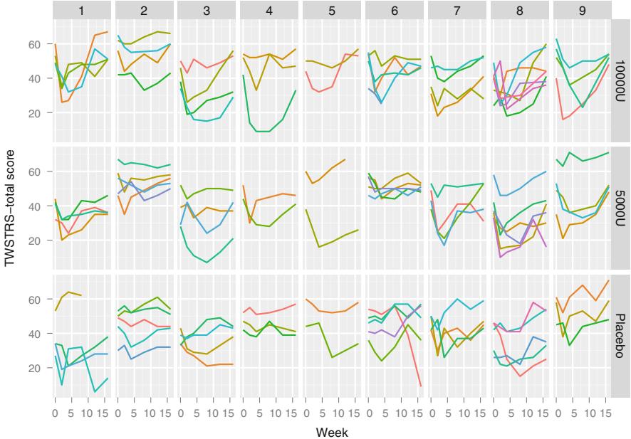

Fig. 7.1 Time profiles for individual subjects, stratified by study site and dose

7.9.2 Using Generalized Least Squares

We stay with baseline adjustment and use a variety of correlation structures, with constant variance. Time is modeled as a restricted cubic spline with 3 knots, because there are only 3 unique interior values of week. Below, six correlation patterns are attempted. In general it is better to use scientific knowledge to guide the choice of the correlation structure.

require( nlme)

cp← list(corCAR1 ,corExp ,corCompSymm ,corLin ,corGaus , corSpher )
z ← vector( ' list ' ,length(cp))
for(k in 1:length(cp)) {
  z[[k]] ← gls(twstrs ∼ treat * rcs(week , 3) +
                rcs(twstrs0 , 3) + rcs(age , 4) * sex , data=both ,
                correlation =cp[[k]](form = ∼week | uid))
}

anova (z[[1]],z[[2]],z[[3]],z[[4]],z[[5]],z[[6]])

z[[6]]	6	20	3570.958	3655.409	-1765.479
z[[5]]	5	20	3621.081	3705.532	-1790.540
z[[4]]	4	20	3575.079	3659.531	-1767.540
z[[3]]	3	20	3587.974	3672.426	-1773.987
z[[2]]	2	20	3553.906	3638.357	-1756.953
z[[1]]	1	20	3553.906	3638.357	-1756.953
	Model	df	AIC	BIC	logLik

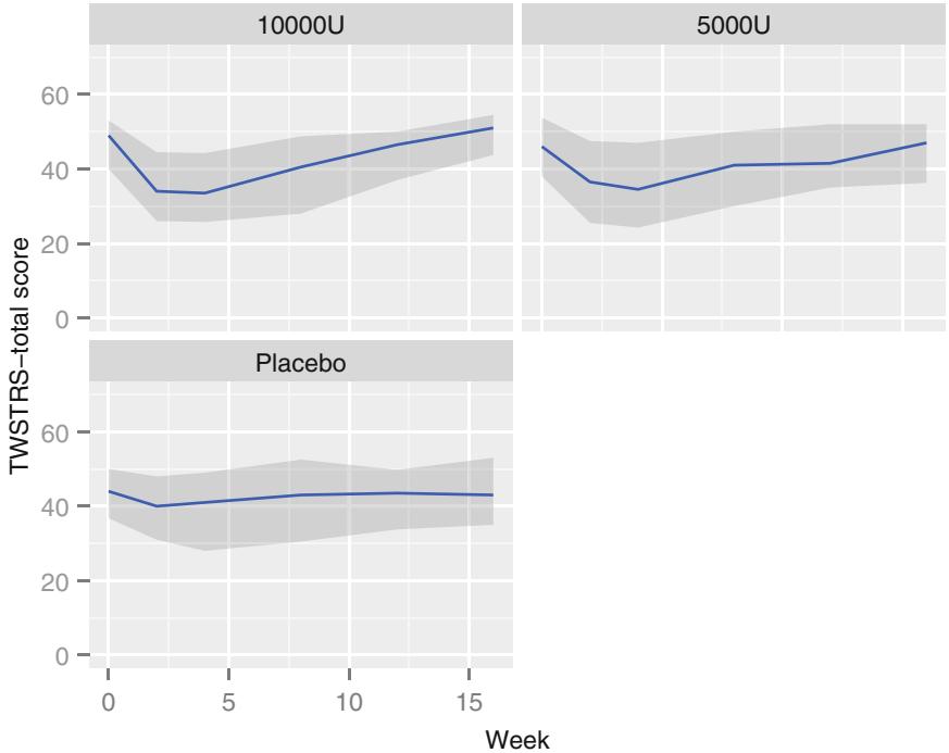
Fig. 7.2 Quartiles of TWSTRS stratified by dose

AIC computed above is set up so that smaller values are best. From this the continuous-time AR1 and exponential structures are tied for the best. ³ For the remainder of the analysis we use corCAR1, using Gls.

a ← Gls(twstrs ∼ treat * rcs(week , 3) + rcs( twstrs0 , 3) +
         rcs(age , 4) * sex , data =both ,
         correlation=corCAR1( form=∼week | uid))

print (a, latex =TRUE)

Generalized Least Squares Fit by REML

Gls(model = twstrs ~ treat * rcs(week, 3) + rcs(twstrs0, 3) + rcs(age, 4) * sex, data = both, correlation = corCAR1 (form = ~week | uid))

Obs 522	Log-restricted-likelihood	-1756.95
Clusters 108	Model d.f.	17
g 11.334	σ	8.5917
	d.f.	504

	Coef	S.E.	t	Pr(> t )
Intercept	-0.3093	11.8804 -0.03		0.9792
treat=5000U	0.4344	2.5962	0.17	0.8672
treat=Placebo	7.1433	2.6133	2.73	0.0065
week	0.2879	0.2973	0.97	0.3334
week’	0.7313	0.3078	2.38	0.0179
twstrs0	0.8071	0.1449	5.57	< 0.0001
twstrs0’	0.2129	0.1795	1.19	0.2360
age	-0.1178	0.2346 -0.50		0.6158
age’	0.6968	0.6484	1.07	0.2830
age”	-3.4018	2.5599 -1.33		0.1845
sex=M	24.2802	18.6208	1.30	0.1929
treat=5000U * week	0.0745	0.4221	0.18	0.8599
treat=Placebo * week	-0.1256	0.4243 -0.30		0.7674
treat=5000U * week’	-0.4389	0.4363 -1.01		0.3149
treat=Placebo * week’	-0.6459	0.4381 -1.47		0.1411
age * sex=M	-0.5846	0.4447 -1.31		0.1892
age’ * sex=M	1.4652	1.2388	1.18	0.2375
age” * sex=M	-4.0338	4.8123 -0.84		0.4023

Correlation Structure: Continuous AR(1)
 Formula: ~week | uid
 Parameter estimate(s):
      Phi
0.8666689

ρˆ = 0.867, the estimate of the correlation between two measurements taken one week apart on the same subject. The estimated correlation for measurements 10 weeks apart is 0.867¹⁰ = 0.24.

v ← Variogram(a, form=∼ week | uid)
plot(v) # Figure 7.3

The empirical variogram is largely in agreement with the pattern dictated by AR(1).

Next check constant variance and normality assumptions.

both$resid ← r ← resid(a); both$fitted ← fitted(a)
yl ← ylab( ' Residuals ' )
p1 ← ggplot(both , aes(x=fitted , y= resid)) + geom_point () +
      facet_grid (∼ treat) + yl
p2 ← ggplot(both , aes(x=twstrs0 , y= resid)) + geom_point ()+yl
p3 ← ggplot(both , aes(x=week , y= resid )) + yl + ylim(-20 ,20) +
      stat_summary( fun.data ="mean_sdl ", geom= ' smooth ' )
p4 ← ggplot(both , aes( sample=resid)) + stat_qq () +
      geom_abline (intercept =mean (r), slope=sd(r)) + yl
gridExtra :: grid.arrange(p1, p2, p3, p4, ncol=2) # Figure 7.4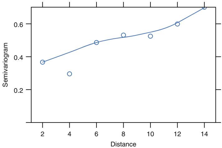

Fig. 7.3 Variogram, with assumed correlation pattern superimposed

These model assumptions appear to be well satisfied, so inferences are likely to be trustworthy if the more subtle multivariate assumptions hold.

Now get hypothesis tests, estimates, and graphically interpret the model.

plot(anova (a)) # Figure 7.5
ylm ← ylim (25, 60)
p1 ← ggplot ( Predict(a, week , treat , conf.int= FALSE),
              adj.subtitle = FALSE , legend.position = ' top ' ) + ylm
p2 ← ggplot ( Predict(a, twstrs0), adj.subtitle = FALSE) + ylm
p3 ← ggplot ( Predict(a, age , sex), adj.subtitle =FALSE ,
              legend.position = ' top ' ) + ylm
gridExtra :: grid.arrange (p1 , p2 , p3 , ncol =2) # Figure 7.6
latex(summary (a),file= ' ' , table.env =FALSE) # Shows for week 8

		Low High ∆		Effect	S.E.		Lower 0.95 Upper 0.95
week	4	12	8		6.69100 1.10570	4.5238	8.8582
twstrs0	39			53 14 13.55100 0.88618		11.8140	15.2880
age	46	65 19			2.50270 2.05140	-1.5179	6.5234
treat — 5000U:10000U	1	2			0.59167 1.99830	-3.3249	4.5083
treat — Placebo:10000U	1	3			5.49300 2.00430	1.5647	9.4212
sex — M:F	1	2		-1.08500 1.77860		-4.5711	2.4011
# To get results for	week	8	for	a	different	reference	group
# for treatment, use	e.g.			summary(a,	week =4,		treat= ’ Placebo ’ )
# Compare low dose	with	placebo ,			separately	at each	time

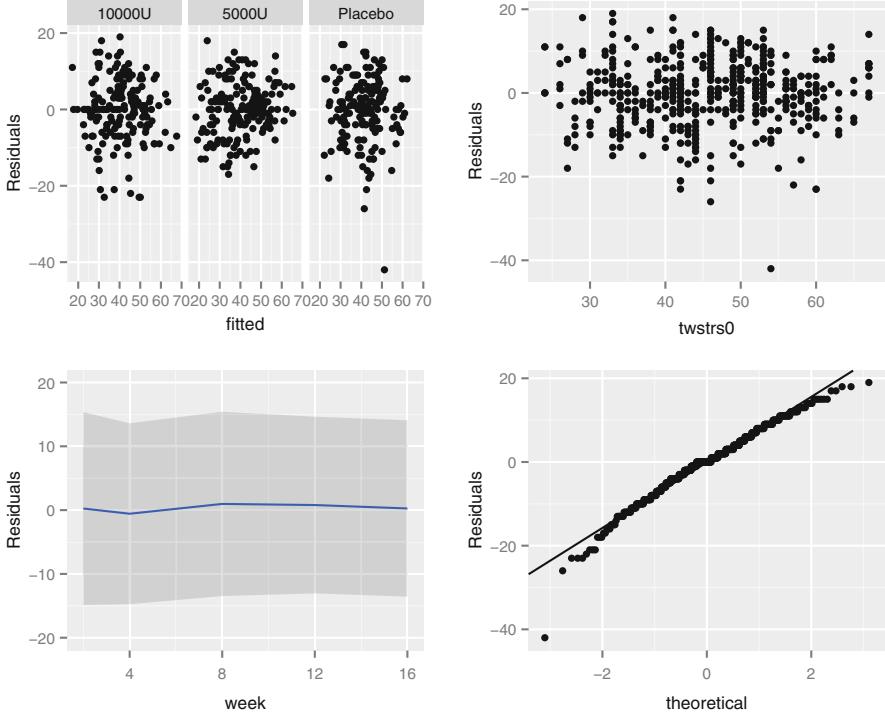
Fig. 7.4 Three residual plots to check for absence of trends in central tendency and in variability. Upper right panel shows the baseline score on the x-axis. Bottom left panel shows the mean ±2×SD. Bottom right panel is the QQ plot for checking normality of residuals from the GLS fit.

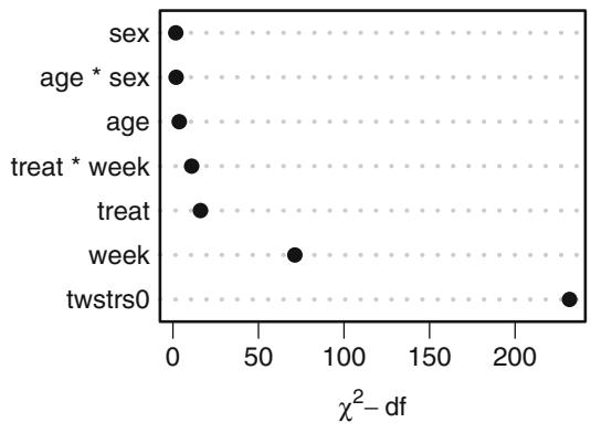
Fig. 7.5 Results of anova from generalized least squares fit with continuous time AR1 correlation structure. As expected, the baseline version of Y dominates.

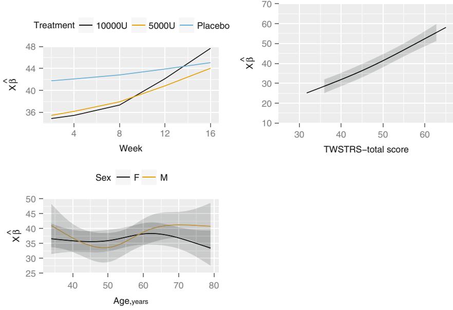
Fig. 7.6 Estimated effects of time, baseline TWSTRS, age, and sex

k1 ← contrast(a, list(week=c(2,4,8,12,16), treat = ' 5000U ' ),
                    list(week=c(2,4,8,12,16), treat = ' Placebo ' ))
options( width =80)
print (k1 , digits =3)

	week	twstrs0	age	sex	Contrast	S.E.	Lower	Upper	Z	Pr(> z )
1	2	46	56	F	-6.31	2.10	-10.43	-2.186	-3.00	0.0027
2	4	46	56	F	-5.91	1.82	-9.47	-2.349	-3.25	0.0011
3	8	46	56	F	-4.90	2.01	-8.85	-0.953	-2.43	0.0150
4*	12	46	56	F	-3.07	1.75	-6.49	0.361	-1.75	0.0795
5*	16	46	56	F	-1.02	2.10	-5.14	3.092	-0.49	0.6260

Redundant contrasts are denoted by *

Confidence intervals are 0.95 individual intervals

# Compare high dose with placebo k2 ← contrast(a, list(week=c(2,4,8,12,16), treat = ’ 10000U ’ ), list(week=c(2,4,8,12,16), treat = ’ Placebo ’ )) print (k2 , digits =3)

week twstrs0 age sex Contrast S.E. Lower Upper Z Pr(>|z|) 1 2 46 56 F -6.89 2.07 -10.96 -2.83 -3.32 0.0009 2 4 46 56 F -6.64 1.79 -10.15 -3.13 -3.70 0.0002 3 8 46 56 F -5.49 2.00 -9.42 -1.56 -2.74 0.0061 4* 12 46 56 F -1.76 1.74 -5.17 1.65 -1.01 0.3109 5* 16 46 56 F 2.62 2.09 -1.47 6.71 1.25 0.2099

Redundant contrasts are denoted by *

Confidence intervals are 0.95 individual intervals

k1 ← as.data.frame (k1[c( ' week ' , ' Contrast ' , ' Lower ' ,
                       ' Upper ' )])
p1 ← ggplot (k1 , aes(x= week , y= Contrast )) + geom_point () +
       geom_line () + ylab( ' Low Dose - Placebo ' ) +
       geom_errorbar (aes( ymin= Lower , ymax=Upper ), width =0)
k2 ← as.data.frame (k2[c( ' week ' , ' Contrast ' , ' Lower ' ,
                       ' Upper ' )])
p2 ← ggplot (k2 , aes(x= week , y= Contrast )) + geom_point () +
       geom_line () + ylab( ' High Dose - Placebo ' ) +
       geom_errorbar (aes( ymin= Lower , ymax=Upper ), width =0)
gridExtra :: grid.arrange (p1 , p2 , ncol =2) # Figure 7.7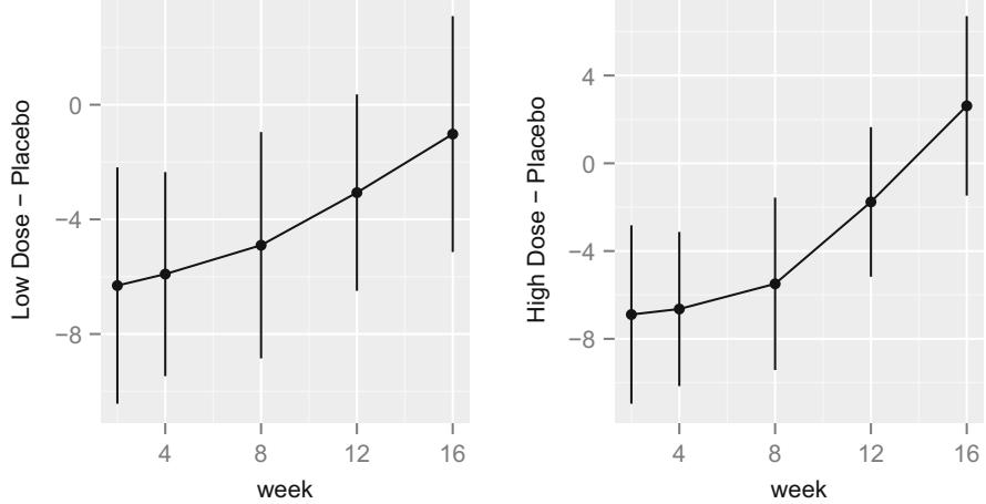

Fig. 7.7 Contrasts and 0.95 confidence limits from GLS fit

Although multiple d.f. tests such as total treatment effects or treatment × time interaction tests are comprehensive, their increased degrees of freedom can dilute power. In a treatment comparison, treatment contrasts at the last time point (single d.f. tests) are often of major interest. Such contrasts are informed by all the measurements made by all subjects (up until dropout times) when a smooth time trend is assumed. They use appropriate extrapolation past dropout times based on observed trajectories of subjects followed the entire observation period. In agreement with the top left panel of Figure 7.6, Figure 7.7 shows that the treatment, despite causing an early improvement, wears off by 16 weeks at which time no benefit is seen.

A nomogram can be used to obtain predicted values, as well as to better understand the model, just as with a univariate Y .

n ← nomogram (a, age=c(seq(20, 80, by =10), 85)) plot(n, cex.axis =.55 , cex.var=.8 , lmgp=.25) # Figure 7.8

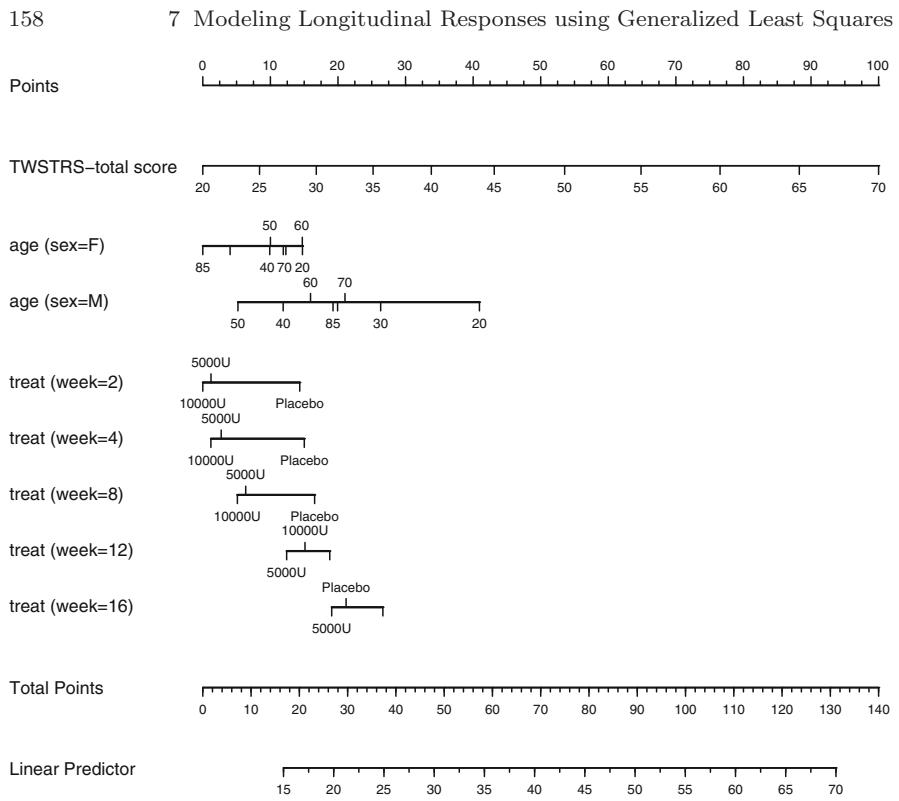
Fig. 7.8 Nomogram from GLS fit. Second axis is the baseline score.

7.10 Further Reading

1 Jim Rochon (Rho, Inc., Chapel Hill NC) has the following comments about using the baseline measurement of Y as the first longitudinal response.

For RCTs [randomized clinical trials], I draw a sharp line at the point when the intervention begins. The LHS [left hand side of the model equation] is reserved for something that is a response to treatment. Anything before this point can potentially be included as a covariate in the regression model. This includes the “baseline” value of the outcome variable. Indeed, the best predictor of the outcome at the end of the study is typically where the patient began at the beginning. It drinks up a lot of variability in the outcome; and, the effect of other covariates is typically mediated through this variable.

I treat anything after the intervention begins as an outcome. In the western scientific method, an “effect” must follow the “cause” even if by a split second.

Note that an RCT is different than a cohort study. In a cohort study, “Time 0” is not terribly meaningful. If we want to model, say, the trend over time, it would be legitimate, in my view, to include the “baseline” value on the LHS of that regression model.

Now, even if the intervention, e.g., surgery, has an immediate effect, I would include still reserve the LHS for anything that might legitimately be considered as the response to the intervention. So, if we cleared a blocked artery and then measured the MABP, then that would still be included on the LHS.

Now, it could well be that most of the therapeutic effect occurred by the time that the first repeated measure was taken, and then levels off. Then, a plot of the means would essentially be two parallel lines and the treatment effect is the distance between the lines, i.e., the difference in the intercepts.

If the linear trend from baseline to Time 1 continues beyond Time 1, then the lines will have a common intercept but the slopes will diverge. Then, the treatment effect will the difference in slopes.

One point to remember is that the estimated intercept is the value at time 0 that we predict from the set of repeated measures post randomization. In the first case above, the model will predict different intercepts even though randomization would suggest that they would start from the same place. This is because we were asleep at the switch and didn’t record the “action” from baseline to time 1. In the second case, the model will predict the same intercept values because the linear trend from baseline to time 1 was continued thereafter.

More importantly, there are considerable benefits to including it as a covariate on the RHS. The baseline value tends to be the best predictor of the outcome post-randomization, and this maneuver increases the precision of the estimated treatment effect. Additionally, any other prognostic factors correlated with the outcome variable will also be correlated with the baseline value of that outcome, and this has two important consequences. First, this greatly reduces the need to enter a large number of prognostic factors as covariates in the linear models. Their effect is already mediated through the baseline value of the outcome variable. Secondly, any imbalances across the treatment arms in important prognostic factors will induce an imbalance across the treatment arms in the baseline value of the outcome. Including the baseline value thereby reduces the need to enter these variables as covariates in the linear models.

Stephen Senn563 states that temporally and logically, a “baseline cannot be a response to treatment”, so baseline and response cannot be modeled in an integrated framework.

. . . one should focus clearly on ‘outcomes’ as being the only values that can be influenced by treatment and examine critically any schemes that assume that these are linked in some rigid and deterministic view to ‘baseline’ values. An alternative tradition sees a baseline as being merely one of a number of measurements capable of improving predictions of outcomes and models it in this way.

The final reason that baseline cannot be modeled as the response at time zero is that many studies have inclusion/exclusion criteria that include cutoffs on the baseline variable yielding a truncated distribution. In general it is not appropriate to model the baseline with the same distributional shape as the follow-up measurements. Thus the approach recommended by Liang and Zeger405 and Liu et al.423 are problematicf .

2 Gardiner et al.211 compared several longitudinal data models, especially with regard to assumptions and how regression coefficients are estimated. Peters et al.500 have an empirical study confirming that the “use all available data” approach of likelihood–based longitudinal models makes imputation of follow-up measurements unnecessary.
3 Keselman et al.347 did a simulation study to study the reliability of AIC for selecting the correct covariance structure in repeated measurement models. In choosing from among 11 structures, AIC selected the correct structure 47% of the time. Gurka et al.247 demonstrated that fixed effects in a mixed effects model can be biased, independent of sample size, when the specified covariate matrix is more restricted than the true one.

^f In addition to this, one of the paper’s conclusions that analysis of covariance is not appropriate if the population means of the baseline variable are not identical in the treatment groups is arguable563. See346 for a discussion of423.

Chapter 8 Case Study in Data Reduction

Recall that the aim of data reduction is to reduce (without using the outcome) the number of parameters needed in the outcome model. The following case study illustrates these techniques:

1. redundancy analysis;
1. variable clustering;
1. data reduction using principal component analysis (PCA), sparse PCA, and pretransformations;
1. restricted cubic spline fitting using ordinary least squares, in the context of scaling; and
1. scaling/variable transformations using canonical variates and nonparametric additive regression.

8.1 Data

Consider the 506-patient prostate cancer dataset from Byar and Green.87 The data are listed in [28, Table 46] and are available in ASCII form from StatLib (lib.stat.cmu.edu) in the Datasets area from this book’s Web page. These data were from a randomized trial comparing four treatments for stage 3 and 4 prostate cancer, with almost equal numbers of patients on placebo and each of three doses of estrogen. Four patients had missing values on all of the following variables: wt, pf, hx, sbp, dbp, ekg, hg, bm; two of these patients were also missing sz. These patients are excluded from consideration. The ultimate goal of an analysis of the dataset might be to discover patterns in survival or to do an analysis of covariance to assess the effect of treatment while adjusting for patient heterogeneity. See Chapter 21 for such analyses. The data reductions developed here are general and can be used for a variety of dependent variables.

The variable names, labels, and a summary of the data are printed below.

require( Hmisc )

getHdata(prostate) # Download and make prostate accessible
# Convert an old date format to R format
prostate$ sdate ← as.Date(prostate$ sdate )
d ← describe(prostate[2:17])
latex (d, file= ' ' )

prostate[2:17] 16 Variables 502 Observations

stage : Stage
     n missing unique Info Mean
   502 0 2 0.73 3.424
  3 (289, 58%), 4 (213, 42%)
rx n missing unique
   502 0 4
  placebo (127, 25%), 0.2 mg estrogen (124, 25%)
  1.0 mg estrogen (126, 25%), 5.0 mg estrogen (125, 25%)
dtime : Months of Follow-up
     n missing unique Info Mean .05 .10 .25 .50 .75 .90 .95
   502 0 76 1 36.13 1.05 5.00 14.25 34.00 57.75 67.00 71.00
  lowest : 0 1 2 3 4, highest: 72 73 74 75 76
status
     n missing unique
   502 0 10
  alive (148, 29%), dead - prostatic ca (130, 26%)
  dead - heart or vascular (96, 19%), dead - cerebrovascular (31, 6%)
  dead - pulmonary embolus (14, 3%), dead - other ca (25, 5%)
  dead - respiratory disease (16, 3%)
  dead - other specific non-ca (28, 6%), dead - unspecified non-ca (7, 1%)
  dead - unknown cause (7, 1%)
age : Age in Years
     n missing unique Info Mean .05 .10 .25 .50 .75 .90 .95
   501 1 41 1 71.46 56 60 70 73 76 78 80
  lowest : 48 49 50 51 52, highest: 84 85 87 88 89
wt : Weight Index = wt(kg)-ht(cm)+200
   n missing unique Info Mean .05 .10 .25 .50 .75 .90 .95 500 2 67 1 99.03 77.95 82.90 90.00 98.00 107.00 116.00 123.00

lowest : 69 71 72 73 74, highest: 136 142 145 150 152

8.1 Data 163
pf
   n missing unique 502 0 4
  normal activity (450, 90%), in bed < 50% daytime (37, 7%)
  in bed > 50% daytime (13, 3%), confined to bed (2, 0%)
hx : History of Cardiovascular Disease
   n missing unique Info Sum Mean 502 0 2 0.73 213 0.4243
sbp : Systolic Blood Pressure/10
   n missing unique Info Mean .05 .10 .25 .50 .75 .90 .95 502 0 18 0.98 14.35 11 12 13 14 16 17 18
             8 9 10 11 12 13 14 15 16 17 18 19 20 21 22 23 24 30
  Frequency 1 3 14 27 65 74 98 74 72 34 17 12 3 2 3 1 1 1
  % 0 1 3 5 13 15 20 15 14 7 3 2 1 0 1 0 0 0
dbp : Diastolic Blood Pressure/10
     n missing unique Info Mean .05 .10 .25 .50 .75 .90 .95
   502 0 12 0.95 8.149 6 6 7 8 9 10 10
             4 5 6 7 8 9 10 11 12 13 14 18
  Frequency 4 5 43 107 165 94 66 9 5 2 1 1
  % 1 1 9 21 33 19 13 2 1 0 0 0
ekg
   n missing unique 494 8 7
  normal (168, 34%), benign (23, 5%)
  rhythmic disturb & electrolyte ch (51, 10%)
  heart block or conduction def (26, 5%), heart strain (150, 30%)
  old MI (75, 15%), recent MI (1, 0%)
hg : Serum Hemoglobin (g/100ml)
   n missing unique Info Mean .05 .10 .25 .50 .75 .90 .95 502 0 91 1 13.45 10.2 10.7 12.3 13.7 14.7 15.8 16.4
  lowest : 5.899 7.000 7.199 7.800 8.199
  highest: 17.297 17.500 17.598 18.199 21.199
sz: Size of Primary Tumor (cm2)
   n missing unique Info Mean .05 .10 .25 .50 .75 .90 .95 497 5 55 1 14.63 2.0 3.0 5.0 11.0 21.0 32.0 39.2
  lowest : 0 1 2 3 4, highest: 54 55 61 62 69
sg : Combined Index of Stage and Hist. Grade
   n missing unique Info Mean .05 .10 .25 .50 .75 .90 .95 491 11 11 0.96 10.31 8 8 9 10 11 13 13
             5 6 7 8 9 10 11 12 13 14 15
  Frequency 3 8 7 67 137 33 114 26 75 5 16
  % 1 2 1 14 28 7 23 5 15 1 3

164 8 Case Study in Data Reduction
ap : Serum Prostatic Acid Phosphatase
    n missing unique Info Mean .05 .10 .25 .50 .75 .90 .95
  502 0 128 1 12.18 0.300 0.300 0.500 0.700 2.975 21.689 38.470
  lowest : 0.09999 0.19998 0.29999 0.39996 0.50000
  highest: 316.00000 353.50000 367.00000 596.00000 999.87500
bm : Bone Metastases
    n missing unique Info Sum Mean
  502 0 2 0.41 82 0.1633

stage is defined by ap as well as X-ray results. Of the patients in stage 3, 0.92 have ap ≤ 0.8. Of those in stage 4, 0.93 have ap > 0.8. Since stage can be predicted almost certainly from ap, we do not consider stage in some of the analyses.

8.2 How Many Parameters Can Be Estimated?

There are 354 deaths among the 502 patients. If predicting survival time were of major interest, we could develop a reliable model if no more than about 354/15 = 24 parameters were examined against Y in unpenalized modeling. Suppose that a full model with no interactions is fitted and that linearity is not assumed for any continuous predictors. Assuming age is almost linear, we could fit a restricted cubic spline function with three knots. For the other continuous variables, let us use five knots. For categorical predictors, the maximum number of degrees of freedom needed would be one fewer than the number of categories. For pf we could lump the last two categories since the last category has only 2 patients. Likewise, we could combine the last two levels of ekg. Table 8.1 lists the candidate predictors with the maximum number of parameters we consider for each.

Table 8.1						Degrees of freedom needed for predictors
———–	–	–	–	–	–	——————————————

Predictor:					rx age wt pf hx sbp dbp ekg hg sz sg ap bm
# Parameters: 3	2	4	2	1	4	4	5	4	4	4	4	1

8.3 Redundancy Analysis

As described in Section 4.7.1, it is occasionally useful to do a rigorous redundancy analysis on a set of potential predictors. Let us run the algorithm discussed there, on the set of predictors we are considering. We will use a low threshold (0.3) for R² for demonstration purposes.

# Allow only 1 d.f. for three of the predictors
prostate ←
  transform (prostate ,
            ekg.norm = 1*(ekg %in% c("normal","benign")),
            rxn = as.numeric (rx),
            pfn = as.numeric (pf))
# Force pfn, rxn to be linear because of difficulty of placing
# knots with so many ties in the data
# Note: all incomplete cases are deleted (inefficient)
redun(∼ stage + I(rxn) + age + wt + I(pfn) + hx +
      sbp + dbp + ekg.norm + hg + sz + sg + ap + bm,
      r2=.3, type= ' adjusted ' , data=prostate )

Redundancy Analysis
redun ( formula = ∼stage + I(rxn) + age + wt + I(pfn) + hx +
   sbp + dbp + ekg.norm + hg + sz + sg + ap + bm ,
   data = prostate , r2 = 0.3, type = " adjusted ")
n: 483 p: 14 nk: 3
Number of NAs: 19
Frequencies of Missing Values Due to Each Variable
  stage I(rxn) age wt I(pfn) hx sbp
dbp
     0012000
0
ekg.norm hg sz sg ap bm
     0 0 5 11 0 0
Transformation of target variables forced to be linear
R2 cutoff : 0.3 Type: adjusted
R2 with which each variable can be predicted from all other
   variables:
  stage I(rxn) age wt I(pfn) hx sbp
dbp
  0.658 0.000 0.073 0.111 0.156 0.062 0.452
0.417
ekg.norm hg sz sg ap bm
  0.055 0.146 0.192 0.540 0.147 0.391
Rendundant variables:
stage sbp bm sg
Predicted from variables:
I(rxn) age wt I(pfn) hx dbp ekg.norm hg sz ap

Variable Deleted R2 R2 after later deletions
1 stage 0.658 0.658 0.646 0.494
2 sbp 0.452 0.453 0.455
3 bm 0.374 0.367
4 sg 0.342

By any reasonable criterion on R2, none of the predictors is redundant. stage can be predicted with an R² = 0.658 from the other 13 variables, but only with R² = 0.493 after deletion of 3 variables later declared to be “redundant.”

8.4 Variable Clustering

From Table 8.1, the total number of parameters is 42, so some data reduction should be considered. We resist the temptation to take the “easy way out” using stepwise variable selection so that we can achieve a more stable modeling ¹ process and obtain unbiased standard errors. Before using a variable clustering procedure, note that ap is extremely skewed. To handle skewness, we use Spearman rank correlations for continuous variables (later we transform each variable using transcan, which will allow ordinary correlation coefficients to be used). After classifying ekg as “normal/benign” versus everything else, the Spearman correlations are plotted below.

x ← with(prostate ,
          cbind (stage , rx , age , wt , pf , hx , sbp , dbp ,
                 ekg.norm , hg , sz , sg , ap , bm))
# If no missing data , could use cor(apply(x, 2, rank ))
r ← rcorr (x, type=" spearman ")$r # rcorr in Hmisc
maxabsr ← max(abs(r[row(r) != col(r)]))

p ← nrow(r)
plot(c(-.35 ,p+.5),c(.5 ,p+.25), type= ' n ' , axes=FALSE ,
     xlab= ' ' ,ylab= ' ' ) # Figure 8.1
v ← dimnames(r )[[1]]
text (rep(.5 ,p), 1:p, v, adj =1)
for(i in 1:(p-1)) {
  for(j in (i+1):p) {
    lines (c(i,i),c(j,j+r[i,j]/ maxabsr/2),
           lwd=3, lend= ' butt ' )
    lines (c(i-.2 ,i+.2),c(j,j), lwd=1, col=gray(.7))
  }
  text(i, i, v[i], srt=-45 , adj =0)
}

We perform a hierarchical cluster analysis based on a similarity matrix that contains pairwise Hoeffding D statistics.295 D will detect nonmonotonic associations.

vc ← varclus(∼ stage + rxn + age + wt + pfn + hx + sbp + dbp + ekg.norm + hg + sz + sg + ap + bm , sim= ’ hoeffding ’ , data= prostate) plot(vc) # Figure 8.2

We combine sbp and dbp, and tentatively combine ap, sg, sz, and bm.

8.5 Transformation and Single Imputation Using transcan

Now we turn to the scoring of the predictors to potentially reduce the number of regression parameters that are needed later by doing away with the need for

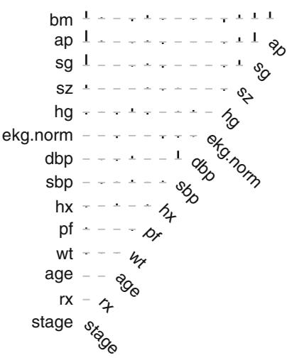
Fig. 8.1 Matrix of Spearman ρ rank correlation coefficients between predictors. Horizontal gray scale lines correspond to ρ = 0. The tallest bar corresponds to |ρ| = 0.78.

nonlinear terms and multiple dummy variables. The R Hmisc package transcan function defaults to using a maximum generalized variance method368 that incorporates canonical variates to optimally transform both sides of a multiple regression model. Each predictor is treated in turn as a variable being predicted, and all variables are expanded into restricted cubic splines (for continuous variables) or dummy variables (for categorical ones).

# Combine 2 levels of ekg (one had freq. 1)
levels ( prostate$ekg)[ levels ( prostate$ekg) %in%
                       c ( ' old MI ' , ' recent MI ' )] ← ' MI '
prostate$pf.coded ← as.integer (prostate$pf)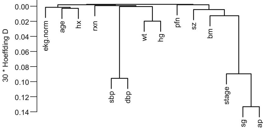

Fig. 8.2 Hierarchical clustering using Hoeffding’s D as a similarity measure. Dummy variables were used for the categorical variable ekg. Some of the dummy variables cluster together since they are by definition negatively correlated.

# make a numeric version; combine last 2 levels of original
levels ( prostate$pf) ← levels ( prostate$pf)[c(1,2,3 ,3)]
ptrans ←
  transcan(∼ sz + sg + ap + sbp + dbp +
            age + wt + hg + ekg + pf + bm + hx , imputed= TRUE ,
            transformed= TRUE , trantab=TRUE , pl=FALSE ,
            show.na=TRUE , data=prostate , frac =.1 , pr=FALSE )
summary( ptrans , digits =4)

transcan (x = ∼sz + sg + ap + sbp + dbp + age + wt + hg + ekg +
   p f + bm + hx , imputed = TRUE, t r an t ab = TRUE, t r an s f o rm e d = TRUE,
   pr = FALSE , p l = FALSE , show . na = TRUE, d ata = p r o s t a t e ,
   frac = 0.1)
Iterations : 8
R2 achieved in predicting each variable :
   s z sg ap sbp dbp age wt hg ekg p f bm hx
0.207 0.556 0.573 0.498 0.485 0.095 0.122 0.158 0.092 0.113 0.349 0.108
Adjusted R2 :
   s z sg ap sbp dbp age wt hg ekg p f bm hx
0.180 0.541 0.559 0.481 0.468 0.065 0.093 0.129 0.059 0.086 0.331 0.083
C o e f f i c i e n t s o f canon i ca l v a r i at e s f or pr ed i c t in g each ( row ) v ar ia b l e
   s z sg ap sbp dbp age wt hg ekg p f bm
sz 0.66 0.20 0.33 0.33 −0.01 −0.01 0.11 0.11 0.03 −0.36
sg 0.23 0.84 0.08 0.07 −0.02 0.01 −0.01 −0.07 0.02 −0.20
ap 0.07 0.80 −0.11 −0.05 0.03 −0.02 0.01 0.01 0.00 −0.83
sbp 0.13 0.10 −0.14 −0.94 0.14 −0.09 0.03 0.10 0.10 −0.03
dbp 0.13 0.09 −0.06 −0.98 0.14 0.07 0.05 0.03 0.04 0.03
age −0.02 −0.06 0.18 0.58 0.57 0.14 0.46 0.43 −0.03 1.05
wt −0.02 0.06 −0.08 −0.31 0.23 0.12 0.51 −0.06 0.21 −1.09
hg 0.13 −0.02 0.03 0.09 0.15 0.33 0.43 −0.02 0.24 −1.53
ekg 0.20 −0.38 0.10 0.42 0.12 0.41 −0.04 −0.04 0.15 −0.42
pf 0.04 0.08 0.02 0.36 0.14 −0.03 0.22 0.29 0.13 −1.75
bm −0.02 −0.03 −0.13 0.00 0.00 0.03 −0.04 −0.06 −0.01 −0.06

hx 0.04 0.05 −0.01 −0.04 0.00 −0.06 0.02 −0.01 −0.09 −0.04 −0.05
   hx
sz 0.34
sg 0.14
ap −0.03
sbp −0.14
dbp −0.01
age −0.76
wt 0 .27
hg −0.12
ekg −1.23
p f −0.46
bm −0.02
hx
Summary o f imputed v a l u e s
s z
     n m i s s i n g un i qu e I n f o Mean
     5 0 4 0.95 12.86
6 ( 2 , 40%) , 7 .416 ( 1 , 20%) , 20 .18 ( 1 , 20%) , 24 .69 ( 1 , 20%)
sg
     n m i s s i n g un i qu e I n f o Mean . 0 5 . 1 0 . 2 5 . 5 0
    11 0 10 1 10.1 6.900 7.289 7.697 10.270
   .75 .90 .95
 10.560 15.000 15.000
         6.511 7.289 7.394 8 10.25 10.27 10.32 10.39 10.73 15
Frequency 1 1 1 1 1 1 1 1 1 2
% 9 9 9 9 9 9 9 9 9 18
age
     n m i s s i n g un i qu e I n f o Mean
     1 0 1 0 71.65
wt
     n m i s s i n g un i qu e I n f o Mean
     2 0 2 1 97.77
91 .24 ( 1 , 50%) , 104 .3 ( 1 , 50%)
ekg
     n m i s s i n g un i qu e I n f o Mean
     8 0 4 0.9 2.625
1 ( 3 , 38%) , 3 ( 3 , 38%) , 4 ( 1 , 12%) , 5 ( 1 , 12%)
Starting estimates for imputed values :
  s z sg ap sbp dbp age wt hg ekg p f bm hx
11.0 10.0 0.7 14.0 8.0 73.0 98.0 13.7 1.0 1.0 0.0 0.0
ggplot (ptrans , scale =TRUE) +

theme( axis.text.x =element_text ( size =6)) # Figure 8.3

The plotted output is shown in Figure 8.3. Note that at face value the transformation of ap was derived in a circular manner, since the combined index of stage and histologic grade, sg, uses in its stage component a cutoff on ap. However, if sg is omitted from consideration, the resulting transformation for ap does not change appreciably. Note that bm and hx are represented as binary variables, so their coefficients in the table of canonical variable coefficients are on a different scale. For the variables that were actually transformed, the coefficients are for standardized transformed variables (mean 0, variance 1). From examining the R²s, age, wt, ekg, pf, and hx are not strongly related to other variables. Imputations for age, wt, ekg are thus relying more on the median or modal values from the marginal distributions. From the coefficients of first (standardized) canonical variates, sbp is predicted almost solely from dbp; bm is predicted mainly from ap, hg, and pf. ²

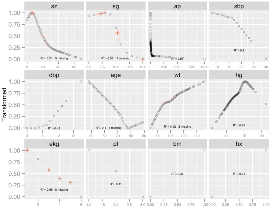
Fig. 8.3 Simultaneous transformation and single imputation of all candidate predictors using transcan. Imputed values are shown as red plus signs. Transformed values are arbitrarily scaled to [0, 1].

8.6 Data Reduction Using Principal Components

The first PC, PC1, is the linear combination of standardized variables having maximum variance. PC² is the linear combination of predictors having the second largest variance such that PC² is orthogonal to (uncorrelated with) PC1. If there are p raw variables, the first k PCs, where k<p, will explain only part of the variation in the whole system of p variables unless one or more of the original variables is exactly a linear combination of the remaining variables. Note that it is common to scale and center variables to have mean zero and variance 1 before computing PCs.

The response variable (here, time until death due to any cause) is not examined during data reduction, so that if PCs are selected by variance explained in the X-space and not by variation explained in Y , one needn’t correct for model uncertainty or multiple comparisons.

PCA results in data reduction when the analyst uses only a subset of the p possible PCs in predicting Y . This is called incomplete principal component regression. When one sequentially enters PCs into a predictive model in a strict pre-specified order (i.e., by descending amounts of variance explained for the system of p variables), model uncertainty requiring bootstrap adjustment is minimized. In contrast, model uncertainty associated with stepwise regression (driven by associations with Y ) is massive.

For the prostate dataset, consider PCs on raw candidate predictors, expanding polytomous factors using dummy variables. The R function princomp is used, after singly imputing missing raw values using transcan’s optimal additive nonlinear models. In this series of analyses we ignore the treatment variable, rx.

# Impute all missing values in all variables given to transcan
imputed ← impute(ptrans , data=prostate , list.out =TRUE)

Imputed missing values with the following frequencies
and stored them in variables with their original names:
sz sg age wt ekg
 5 11 1 2 8

imputed ← as.data.frame (imputed)
# Compute principal components on imputed data.
# Create a design matrix from ekg categories
Ekg ← model.matrix (∼ ekg , data=imputed )[, -1]
# Use correlation matrix
pfn ← prostate$pfn
prin.raw ← princomp(∼ sz + sg + ap + sbp + dbp + age +
                       wt + hg + Ekg + pfn + bm + hx,
                       cor=TRUE , data= imputed)
plot(prin.raw , type= ' lines ' , main= ' ' , ylim=c(0,3)) #Figure 8.4
# Add cumulative fraction of variance explained
addscree ← function(x, npcs=min(10, length (x$sdev )),
                       plotv= FALSE ,
                       col=1, offset =.8 , adj=0, pr=FALSE ) {
  vars ← x$sdev∧2
  cumv ← cumsum (vars)/sum(vars)
  if(pr) print (cumv)
  text (1: npcs , vars[1:npcs] + offset *par( ' cxy ' )[2],
       as.character ( round (cumv [1:npcs], 2)),
       srt=45, adj=adj , cex=.65 , xpd=NA , col=col)
  if(plotv ) lines (1: npcs , vars[1:npcs], type= ' b ' , col=col)
}
addscree(prin.raw)
prin.trans ← princomp( ptrans $transformed , cor= TRUE)
addscree( prin.trans , npcs =10, plotv =TRUE , col= ' red ' ,
         offset =-.8 , adj =1)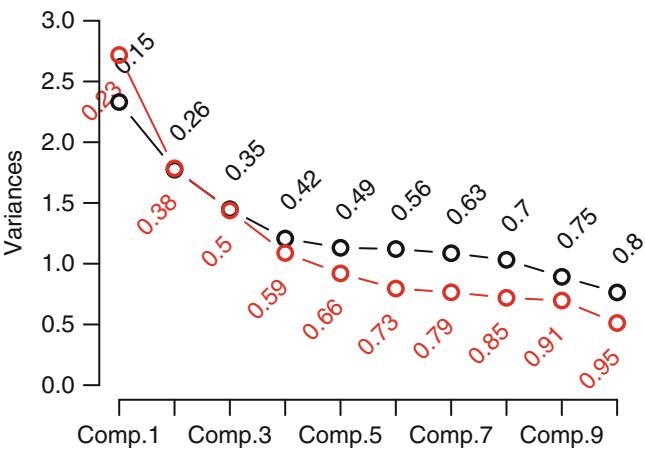

Fig. 8.4 Variance of the system of raw predictors (black) explained by individual principal components (lines) along with cumulative proportion of variance explained (text), and variance explained by components computed on transcan-transformed variables (red)

The resulting plot shown in Figure 8.4 is called a “scree” plot [325, pp. 96–99, 104, 106]. It shows the variation explained by the first k principal components as k increases all the way to 16 parameters (no data reduction). It requires 10 of the 16 possible components to explain > 0.8 of the variance, and the first 5 components explain 0.49 of the variance of the system. Two of the 16 dimensions are almost totally redundant.

After repeating this process when transforming all predictors via transcan, we have only 12 degrees of freedom for the 12 predictors. The variance explained is depicted in Figure 8.4 in red. It requires at least 9 of the 12 possible components to explain ≥ 0.9 of the variance, and the first 5 components explain 0.66 of the variance as opposed to 0.49 for untransformed variables.

Let us see how the PCs “explain” the times until death using the Cox regression132 function from rms, cph, described in Chapter 20. In what follows we vary the number of components used in the Cox models from 1 to all 16, computing the AIC for each model. AIC is related to model log likelihood penalized for number of parameters estimated, and lower is better. For reference, the AIC of the model using all of the original predictors, and the AIC of a full additive spline model are shown as horizontal lines.

require(rms)

S ← with(prostate , Surv( dtime , status != "alive "))
# two-column response var.
pcs ← prin.raw$ scores # pick off all PCs
aic ← numeric (16)
for(i in 1:16) {

ps ← pcs[,1:i]
  aic[i] ← AIC(cph(S ∼ ps))
} # Figure 8.5
plot (1:16, aic , xlab= ' Number of Components Used ' ,
     ylab= ' AIC ' , type= ' l ' , ylim=c(3950 ,4000))
f ← cph(S ∼ sz + sg + log(ap) + sbp + dbp + age + wt + hg +
         ekg + pf + bm + hx , data = imputed)
abline (h=AIC(f), col= ' blue ' )
f ← cph(S ∼ rcs(sz ,5) + rcs(sg ,5) + rcs(log(ap),5) +
         rcs(sbp ,5) + rcs(dbp ,5) + rcs(age ,3) + rcs(wt ,5) +
         rcs(hg ,5) + ekg + pf + bm + hx ,
         tol=1e-14 , data= imputed)

abline (h=AIC(f), col= ' blue ' , lty=2)

For the money, the first 5 components adequately summarizes all variables, if linearly transformed, and the full linear model is no better than this. The model allowing all continuous predictors to be nonlinear is not worth its added degrees of freedom.

Next check the performance of a model derived from cluster scores of transformed variables.

# Compute PC1 on a subset of transcan-transformed predictors
pco ← function(v) {
  f ← princomp( ptrans $ transformed [,v], cor= TRUE)
  vars ← f$sdev∧2
  cat( ' Fraction of variance explained by PC1: ' ,
      round (vars [1]/sum(vars),2), ' \ n ' )
  f$scores [,1]
}
tumor ← pco(c( ' sz ' , ' sg ' , ' ap ' , ' bm ' ))

Fraction of variance explained by PC1: 0.59

bp ← pco(c( ’ sbp ’ , ’ dbp ’ ))

Fraction of variance explained by PC1: 0.84

cardiac ← pco(c( ’ hx ’ , ’ ekg ’ ))

Fraction of variance explained by PC1: 0.61

# Get transformed individual variables that are not clustered other ← ptrans$transformed [,c( ’ hg ’ , ’ age ’ , ’ pf ’ , ’ wt ’ )] f ← cph(S ∼ tumor + bp + cardiac + other) # other is matrix AIC(f)

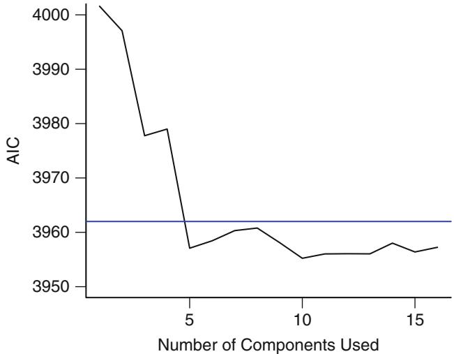
Fig. 8.5 AIC of Cox models fitted with progressively more principal components. The solid blue line depicts the AIC of the model with all original covariates. The dotted blue line is positioned at the AIC of the full spline model.

		Model Tests			Discrimination
					Indexes
Obs	502	χ2 LR	81.11	R2	0.149
Events 354		d.f.	7	Dxy	0.286
Center	0	χ2) Pr(>	0.0000	g	0.562
		χ2 Score	86.81	gr	1.755
		χ2) Pr(>	0.0000

	Coef	S.E.	Wald Z	Pr(> Z )
tumor	-0.1723	0.0367	-4.69	< 0.0001
bp	-0.0251	0.0424	-0.59	0.5528
cardiac	-0.2513	0.0516	-4.87	< 0.0001
hg	-0.1407	0.0554	-2.54	0.0111
age	-0.1034	0.0579	-1.79	0.0739
pf	-0.0933	0.0487	-1.92	0.0551
wt	-0.0910	0.0555	-1.64	0.1012

The tumor and cardiac clusters seem to dominate prediction of mortality, and the AIC of the model built from cluster scores of transformed variables compares favorably with other models (Figure 8.5).

8.6.1 Sparse Principal Components

A disadvantage of principal components is that every predictor receives a nonzero weight for every component, so many coefficients are involved even through the effective degrees of freedom with respect to the response model are reduced. Sparse principal components672 uses a penalty function to reduce the magnitude of the loadings variables receive in the components. If an L1 penalty is used (as with the lasso), some loadings are shrunk to zero, resulting in some simplicity. Sparse principal components combines some elements of variable clustering, scoring of variables within clusters, and redundancy analysis.

Filzmoser, Fritz, and Kalcher191 have written a nice R package pcaPP for doing sparse PC analysis.a The following example uses the prostate data again. To allow for nonlinear transformations and to score the ekg variable in the prostate dataset down to a scalar, we use the transcan-transformed predictors as inputs.

require( pcaPP )

s ← sPCAgrid( ptrans $transformed , k=10, method = ' sd ' ,
               center = mean , scale =sd , scores =TRUE ,
               maxiter =10)
plot(s, type= ' lines ' , main= ' ' , ylim=c(0,3)) # Figure 8.6
addscree(s)
s$loadings # These loadings are on the orig. transcan scale

Loadings : Comp . 1 sz 0.248 sg 0.620 ap 0.634	Comp . 2		Comp . 3 Comp . 4	Comp . 5		Comp . 6	Comp . 7	Comp . 8 Comp . 9	0.950	Comp . 1 0 0.522
sbp	−0.707								−0.305
dbp		0.707
age				1.000
wt							1.000
hg						1.000
ekg								1.000
pf			1.000
bm −0.391										0.852
hx					1.000
		Comp . 1	Comp . 2	Comp . 3	Comp . 4	Comp . 5	Comp . 6	Comp . 7	Comp . 8
SS l oad ings		1.000	1.000	1.000	1.000	1.000	1.000	1.000	1.000
Proport ion	Var	0.083	0.083	0.083	0.083	0.083	0.083	0.083	0.083
Cumulative	Var	0.083	0.167	0.250	0.333	0.417	0.500	0.583	0.667
		Comp . 9	Comp . 1 0
SS l oad ings		1.000	1.000
Proport ion	Var	0.083	0.083
Cumulative	Var	0.750	0.833

Only nonzero loadings are shown. The first sparse PC is the tumor cluster used above, and the second is the blood pressure cluster. Let us see how well incomplete sparse principal component regression predicts time until death.

^a The spca package is a new sparse PC package that should also be considered.

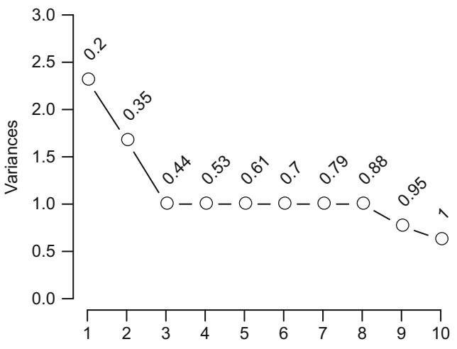
Fig. 8.6 Variance explained by individual sparse principal components (lines) along with cumulative proportion of variance explained (text)

pcs ← s$scores # pick off sparse PCs
aic ← numeric (10)
for(i in 1:10) {
  ps ← pcs[,1:i]
  aic[i] ← AIC(cph(S ∼ ps))
} # Figure 8.7
plot (1:10, aic , xlab= ' Number of Components Used ' ,
     ylab= ' AIC ' , type= ' l ' , ylim=c(3950 ,4000))

More components are required to optimize AIC than were seen in Figure 8.5, but a model built from 6–8 sparse PCs performed as well as the other models.

8.7 Transformation Using Nonparametric Smoothers

The ACE nonparametric additive regression method of Breiman and Friedman68 transforms both the left-hand-side variable and all the right-hand-side variables so as to optimize R². ACE can be used to transform the predictors using the R ace function in the acepack package, called by the transace function in the Hmisc package. transace does not impute data but merely does casewise deletion of missing values. Here transace is run after single imputation by transcan. binary is used to tell transace which variables not to try to predict (because they need no transformation). Several predictors are restricted to be monotonically transformed.

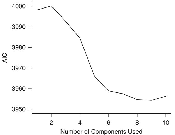
Fig. 8.7 Performance of sparse principal components in Cox models

x ← with(imputed ,
          cbind (sz , sg , ap , sbp , dbp , age , wt , hg , ekg , pf,
                 bm , hx))
monotonic ← c("sz","sg","ap","sbp","dbp","age","pf")
transace(x, monotonic , # Figure 8.8
         categorical ="ekg", binary =c("bm","hx"))

R2 achieved in predicting each variable :
     sz sg ap sbp dbp age wt
0.2265824 0.5762743 0.5717747 0.4823852 0.4580924 0.1514527 0.1732244
     hg ekg p f bm hx
0 . 2 0 0 1 0 0 8 0 . 1 1 1 0 7 0 9 0 . 1 7 7 8 7 0 5 NA NA

Except for ekg, age, and for arbitrary sign reversals, the transformations in Figure 8.8 determined using transace were similar to those in Figure 8.3. The transcan transformation for ekg makes more sense.

8.8 Further Reading

1 Sauerbrei and Schumacher541 used the bootstrap to demonstrate the variability of a standard variable selection procedure for the prostate cancer dataset.
2 Schemper and Heinze551 used logistic models to impute dichotomizations of the predictors for this dataset.

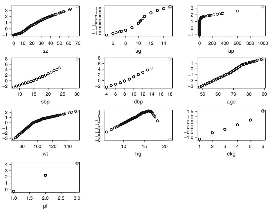
Fig. 8.8 Simultaneous transformation of all variables using ACE.

8.9 Problems

The Mayo Clinic conducted a randomized trial in primary biliary cirrhosis (PBC) of the liver between January 1974 and May 1984, to compare Dpenicillamine with placebo. The drug was found to be ineffective [197, p. 2], and the trial was done before liver transplantation was common, so this trial constitutes a natural history study for PBC. Followup continued through July, 1986. For the 19 patients that did undergo transplant, followup time was censored (status=0) at the day of transplant. 312 patients were randomized, and another 106 patients were entered into a registry. The nonrandomized patients have most of their laboratory values missing, except for bilirubin, albumin, and prothrombin time. 28 randomized patients had both serum cholesterol and triglycerides missing. The data, which consist of clinical, biochemical, serologic, and histologic information, are listed in [197, pp. 359– 375]. The PBC data are discussed and analyzed in [197, pp. 2–7, 102–104, 153–162], [158], [7] (a tree-based analysis which on its p. 480 mentions some possible lack of fit of the earlier analyses), and [361]. The data are stored in the datasets web site so may be accessed using the Hmisc getHdata function with argument pbc. Use only the data on randomized patients for all analyses. For Problems 1–6, ignore followup time, status, and drug.

1. Do an initial variable clustering based on ranks, using pairwise deletion of missing data. Comment on the potential for one-dimensional summaries of subsets of variables being adequate summaries of prognostic information.
1. cholesterol, triglycerides, platelets, and copper are missing on some patients. Impute them using a method you recommend. Use some or all of the remaining predictors and possibly the outcome. Provide a correlation coefficient describing the usefulness of each imputation model. Provide the actual imputed values, specifying observation numbers. For all later analyses, use imputed values for missing values.
1. Perform a scaling/transformation analysis to better measure how the predictors interrelate and to possibly pretransform some of them. Use transcan or ACE. Repeat the variable clustering using the transformed scores and Pearson correlation or using an oblique rotation principal component analysis. Determine if the correlation structure (or variance explained by the first principal component) indicates whether it is possible to summarize multiple variables into single scores.
1. Do a principal component analysis of all transformed variables simultaneously. Make a graph of the number of components versus the cumulative proportion of explained variation. Repeat this for laboratory variables alone.
1. Repeat the overall PCA using sparse principal components. Pay attention to how best to solve for sparse components, e.g., consider the lambda parameter in sPCAgrid.
1. How well can variables (lab and otherwise) that are routinely collected (on nonrandomized patients) capture the information (variation) of the variables that are often missing? It would be helpful to explore the strength of interrelationships by
- 1. correlating two PC1s obtained from untransformed variables,
- 1. correlating two PC1s obtained from transformed variables,
- 1. correlating the best linear combination of one set of variables with the best linear combination of the other set, and
- 1. doing the same on transformed variables.

For this problem consider only complete cases, and transform the 5 nonnumeric categorical predictors to binary 0–1 variables.

1. Consider the patients having complete data who were randomized to placebo. Consider only models that are linear in all the covariates.
- 1. Fit a survival model to predict time of death using the following covariates: bili, albumin, stage, protime, age, alk.phos, sgot, chol, trig, platelet, copper.
- 1. Perform an ordinary principal component analysis. Fit the survival model using only the first 3 PCs. Compare the likelihood ratio χ² and AIC with that of the model using the original variables.
1. Considering the PCs are fixed, use the bootstrap to estimate the 0.95 confidence interval of the inter-quartile-range age effect on the original scale, and the same type of confidence interval for the coefficient of PC1.
1. Now accounting for uncertainty in the PCs, compute the same two confidence intervals. Compare and interpret the two sets. Take into account the fact that PCs are not unique to within a sign change.

R programming hints for this exercise are found on the course web site.

Chapter 9 Overview of Maximum Likelihood Estimation

9.1 General Notions—Simple Cases

In ordinary least squares multiple regression, the objective in fitting a model is to find the values of the unknown parameters that minimize the sum of squared errors of prediction. When the response variable is non-normal, polytomous, or not observed completely, one needs a more general objective function to optimize.

Maximum likelihood (ML) estimation is a general technique for estimating parameters and drawing statistical inferences in a variety of situations, especially nonstandard ones. Before laying out the method in general, ML estimation is illustrated with a standard situation, the one-sample binomial problem. Here, independent binary responses are observed and one wishes to draw inferences about an unknown parameter, the probability of an event in a population.

Suppose that in a population of individuals, each individual has the same probability P that an event occurs. We could also say that the event has already been observed, so that P is the prevalence of some condition in the population. For each individual, let Y = 1 denote the occurrence of the event and Y = 0 denote nonoccurrence. Then Prob{Y = 1} = P for each individual. Suppose that a random sample of size 3 from the population is drawn and that the first individual had Y = 1, the second had Y = 0, and the third had Y = 1. The respective probabilities of these outcomes are P, 1−P, and P. The joint probability of observing the independent events Y = 1, 0, 1 is ^P(1 ⁻ ^P)^P ⁼ ^P²(1 ⁻ ^P). Now the value of ^P is unknown, but we can solve for the value of P that makes the observed data (Y = 1, 0, 1) most likely to have occurred. In this case, the value of ^P that maximizes ^P²(1 ⁻ ^P) is P = 2/3. This value for P is the maximum likelihood estimate (MLE) of the population probability.

F.E. Harrell, Jr., Regression Modeling Strategies, Springer Series in Statistics, DOI 10.1007/978-3-319-19425-7 9

Let us now study the situation of independent binary trials in general. Let the sample size be n and the observed responses be Y1, Y2,…,Yn. The joint probability of observing the data is given by

\[L = \prod\_{i=1}^{n} P^{Y\_i} (1 - P)^{1 - Y\_i}. \tag{9.1}\]

Now let s denote the sum of the Y s or the number of times that the event occurred (Yⁱ = 1), that is the number of “successes.” The number of nonoccurrences (“failures”) is n − s. The likelihood of the data can be simplified to

\[L = P^s (1 - P)^{n - s}.\tag{9.2}\]

It is easier to work with the log likelihood function, which also has desirable statistical properties. For the one-sample binary response problem, the log likelihood is

\[ \log L = s \log(P) + (n - s) \log(1 - P). \tag{9.3} \]

The MLE of P is that value of P that maximizes L or log L. Since log L is a smooth function of P, its maximum value can be found by finding the point at which log L has a slope of 0. The slope or first derivative of logL, with respect to P, is

\[U(P) = \partial \log L / \partial P = s / P - (n - s) / (1 - P). \tag{9.4}\]

The first derivative of the log likelihood function with respect to the parameter(s), here U(P), is called the score function. Equating this function to zero requires that s/P = (n − s)/(1 − P). Multiplying both sides of the equation by P(1 − P) yields s(1 − P)=(n − s)P or that s = (n − s)P + sP = nP. Thus the MLE of P is p = s/n.

Another important function is called the Fisher information about the unknown parameters. The information function is the expected value of the negative of the curvature in log L, which is the negative of the slope of the slope as a function of the parameter, or the negative of the second derivative of log L. Motivation for consideration of the Fisher information is as follows. If the log likelihood function has a distinct peak, the sample provides information that allows one to readily discriminate between a good parameter estimate (the location of the obvious peak) and a bad one. In such a case the MLE will have good precision or small variance. If on the other hand the likelihood function is relatively flat, almost any estimate will do and the chosen estimate will have poor precision or large variance. The degree of peakedness of a function at a given point is the speed with which the slope is changing at that point, that is, the slope of the slope or second derivative of the function at that point.

9.1 General Notions—Simple Cases 183

Here, the information is

\[\begin{split} I(P) &= E\{-\partial^2 \log L / \partial P^2\} \\ &= E\{s/P^2 + (n-s)/(1-P)^2\} \\ &= nP/P^2 + n(1-P)/(1-P)^2 = n/[P(1-P)]. \end{split} \tag{9.5}\]

We estimate the information by substituting the MLE of P into I(P), yielding I(p) = n/[p(1 − p)].

Figures 9.1, 9.2, and 9.3 depict, respectively, log L, U(P), and I(P), all as a function of P. Three combinations of n and s were used in each graph. These combinations correspond to p = .5, .6, and .6, respectively.

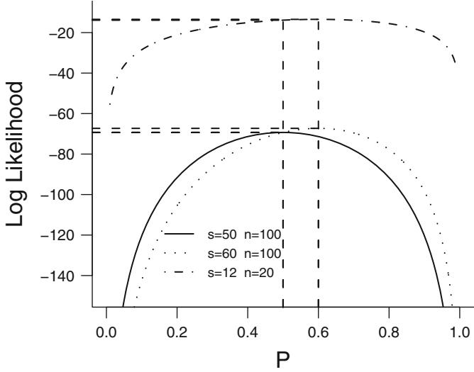
Fig. 9.1 log likelihood functions for three one-sample binomial problems

In each case it can be seen that the value of P that makes the data most likely to have occurred (the value that maximizes L or log L) is p given above. Also, the score function (slope of log L) is zero at P = p. Note that the information function I(P) is highest for P approaching 0 or 1 and is lowest for P near .5, where there is maximum uncertainty about P. Note also that while log L has the same shape for the s = 60 and s = 12 curves in Figure 9.1, the range of log L is much greater for the larger sample size. Figures 9.2 and 9.3 show that the larger sample size produces a sharper likelihood. In other words, with larger n, one can zero in on the true value of P with more precision.

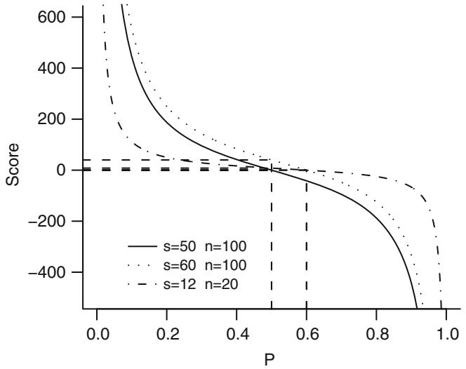
Fig. 9.2 Score functions (∂L/∂P)

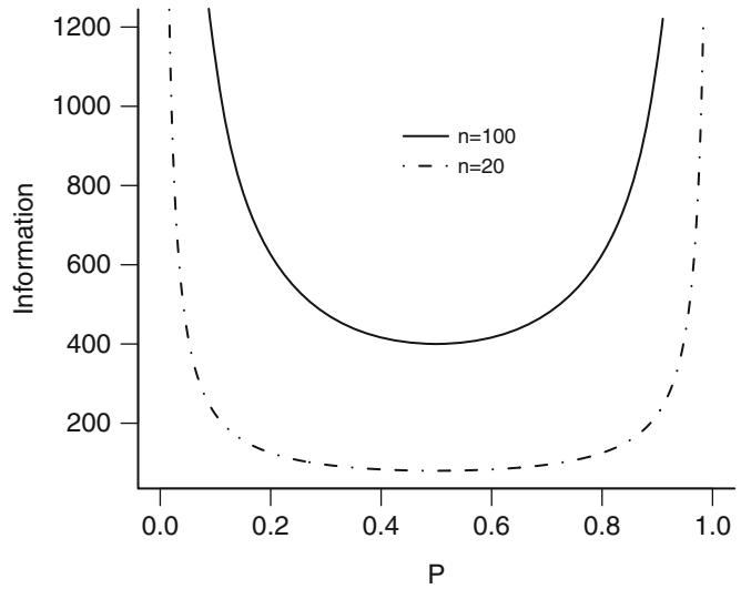
Fig. 9.3 Information functions (−∂² log L/∂^P ²)

In this binary response one-sample example let us now turn to inference about the parameter P. First, we turn to the estimation of the variance of the MLE, p. An estimate of this variance is given by the inverse of the information at P = p:

\[Var(p) = I(p)^{-1} = p(1-p)/n.\tag{9.6}\]

Note that the variance is smallest when the information is greatest (p = 0 or 1).

The variance estimate forms a basis for confidence limits on the unknown parameter. For large n, the MLE p is approximately normally distributed with expected value (mean) P and variance P(1 − P)/n. Since p(1 − p) is a consistent estimate of P(1 − P)/n, it follows that p ± z[p(1 − p)/n] ¹/² is an approximate 1 − α confidence interval for P if z is the 1 − α/2 critical value of the standard normal distribution.

9.2 Hypothesis Tests

Now let us turn to hypothesis tests about the unknown population parameter P — H⁰ : P = P0. There are three kinds of statistical tests that arise from likelihood theory.

9.2.1 Likelihood Ratio Test

This test statistic is the ratio of the likelihood at the hypothesized parameter values to the likelihood of the data at the maximum (i.e., at parameter values = MLEs). It turns out that −2× the log of this likelihood ratio has desirable statistical properties. The likelihood ratio test statistic is given by

\[\begin{split} LR &= -2\log(L \text{ at } H\_0/L \text{ at MLEs}) \\ &= -2(\log L \text{ at } H\_0) - [-2(\log L \text{ at MLEs})]. \end{split} \tag{9.7}\]

The LR statistic, for large enough samples, has approximately a χ² distribution with degrees of freedom equal to the number of parameters estimated, if the null hypothesis is “simple,” that is, doesn’t involve any unknown parameters. Here LR has 1 d.f.

The value of log L at H⁰ is

\[\log L(H\_0) = s \log(P\_0) + (n - s) \log(1 - P\_0). \tag{9.8}\]

The maximum value of log L (at MLEs) is

\[ \log L(P=p) = s \log(p) + (n-s) \log(1-p). \tag{9.9} \]

For the hypothesis H⁰ : P = P0, the test statistic is

\[LR = -2\{s\log(P\_0/p) + (n-s)\log[(1-P\_0)/(1-p)]\}.\tag{9.10}\]

Note that when p happens to equal P0, LR = 0. When p is far from P0, LR will be large. Suppose that P⁰ = 1/2, so that H⁰ is P = 1/2. For n = 100, s = 50, LR = 0. For n = 100, s = 60,

\[LR = -2\{60\log(.5/.6) + 40\log(.5/.4)\} = 4.03.\tag{9.11}\]

For n = 20, s = 12,

\[LR = -2\{12\log(.5/.6) + 8\log(.5/.4)\} = .81 = 4.03/5. \tag{9.12}\]

Therefore, even though the best estimate of P is the same for these two cases, the test statistic is more impressive when the sample size is five times larger.

9.2.2 Wald Test

The Wald test statistic is a generalization of a t- or z-statistic. It is a function of the difference in the MLE and its hypothesized value, normalized by an estimate of the standard deviation of the MLE. Here the statistic is

\[W = [p - P\_0]^2 / [p(1 - p) / n]. \tag{9.13}\]

For large enough n, W is distributed as χ² with 1 d.f. For n = 100, s = 50, W = 0. For the other samples, W is, respectively, 4.17 and 0.83 (note 0.83 = 4.17/5).

Many statistical packages treat ^√^W as having a ^t distribution instead of a normal distribution. As pointed out by Gould,228 there is no basis for this outside of ordinary linear modelsa.

9.2.3 Score Test

If the MLE happens to equal the hypothesized value P0, P⁰ maximizes the likelihood and so U(P0) = 0. Rao’s score statistic measures how far from zero the score function is when evaluated at the null hypothesis. The score function

^a In linear regression, a t distribution is used to penalize for the fact that the variance of Y |X is estimated. In models such as the logistic model, there is no separate variance parameter to estimate. Gould has done simulations that show that the normal distribution provides more accurate P-values than the t for binary logistic regression.

(slope or first derivative of log L) is normalized by the information (curvature or second derivative of − logL). The test statistic for our example is

\[S = U(P\_0)^2 / I(P\_0),\tag{9.14}\]

which formally does not involve the MLE, p. The statistic can be simplified as follows.

\[\begin{aligned} U(P\_0) &= s/P\_0 - (n-s)/(1-P\_0) \\ I(P\_0) &= s/P\_0^2 + (n-s)/(1-P\_0)^2 \\ S &= \left(s - nP\_0\right)^2/[nP\_0(1-P\_0)] = n(p-P\_0)^2/[P\_0(1-P\_0)].\end{aligned} \tag{9.15}\]

Note that the numerator of S involves s − nP0, the difference between the observed number of successes and the number of successes expected under H0.

As with the other two test statistics, S = 0 for the first sample. For the last two samples S is, respectively, 4 and .8 = 4/5. ¹

9.2.4 Normal Distribution—One Sample

Suppose that a sample of size n is taken from a population for a random variable Y that is known to be normally distributed with unknown mean µ and variance σ². Denote the observed values of the random variable by Y1, Y2,…,Yn. Now unlike the binary response case (Y = 0 or 1), we cannot use the notion of the probability that Y equals an observed value. This is because Y is continuous and the probability that it will take on a given value is zero. We substitute the density function for the probability. The density at a point y is the limit as d approaches zero of

\[\text{Prob}\{y < Y \le y + d\}/d = [F(y+d) - F(y)]/d,\tag{9.16}\]

where F(y) is the normal cumulative distribution function (for a mean of µ and variance of σ²). The limit of the right-hand side of the above equation as d approaches zero is f(y), the density function of a normal distribution with mean µ and variance σ². This density function is

\[f(y) = (2\pi\sigma^2)^{-1/2} \exp\{- (y-\mu)^2 / 2\sigma^2\}.\tag{9.17}\]

The likelihood of observing the observed sample values is the joint density of the Y s. The log likelihood function here is a function of two unknowns, µ and σ².

\[\log L = -.5n \log \left( 2\pi \sigma^2 \right) - .5 \sum\_{i=1}^{n} (Y\_i - \mu)^2 / \sigma^2. \tag{9.18}\]

It can be shown that the value of µ that maximizes log L is the value that minimizes the sum of squared deviations about µ, which is the sample mean Y . The MLE of σ² is

\[s^2 = \sum\_{i=1}^{n} (Y\_i - \overline{Y})^2 / n. \tag{9.19}\]

Recall that the sample variance uses n−1 instead of n in the denominator. It can be shown that the expected value of the MLE of ^σ2, ^s2, is [(ⁿ ⁻ 1)/n]σ2; in other words, ^s² is too small by a factor of (ⁿ ⁻ 1)/n on the average. The sample variance is unbiased, but being unbiased does not necessarily make it a better estimator. The MLE has greater precision (smaller mean squared error) in many cases.

9.3 General Case

Suppose we need to estimate a vector of unknown parameters B = {B1, B2, …,Bp} from a sample of size n based on observations Y1,…,Yn. Denote the probability or density function of the random variable Y for the ith observation by fi(y; B). The likelihood for the ith observation is Li(B) = fi(Yi; B). In the one-sample binary response case, recall that Li(B) = Li(P) = ^P ^Yⁱ [1 ⁻ ^P] ¹−Yⁱ . The likelihood function, or joint likelihood of the sample, is given by

\[L(B) = \prod\_{i=1}^{n} f\_i(Y\_i; B). \tag{9.20}\]

The log likelihood function is

\[\log L(B) = \sum\_{i=1}^{n} \log L\_i(B). \tag{9.21}\]

The MLE of B is that value of the vector B that maximizes log L(B) as a function of B. In general, the solution for B requires iterative trial-anderror methods as outlined later. Denote the MLE of B as b = {b1,…,bp}. The score vector is the vector of first derivatives of log L(B) with respect to B1,…,Bp:

\[\begin{split} U(B) &= \{ \partial / \partial B\_1 \log L(B), \dots, \partial / \partial B\_p \log L(B) \} \\ &= (\partial / \partial B) \log L(B). \end{split} \tag{9.22}\]

The Fisher information matrix is the p × p matrix whose elements are the negative of the expectation of all second partial derivatives of logL(B):

\[\begin{split} I^\*(B) &= -\{ E[ (\partial^2 \log L(B) / \partial B\_j \partial B\_k) ] \}\_{p \times p} \\ &= -E\{ (\partial^2 / \partial B \partial B') \log L(B) \}. \end{split} \tag{9.23}\]

The observed information matrix I(B) is I∗(B) without taking the expectation. In other words, observed values remain in the second derivatives:

\[I(B) = - (\partial^2 / \partial B \partial B^\prime) \log L(B). \tag{9.24}\]

This information matrix is often estimated from the sample using the estimated observed information I(b), by inserting b, the MLE of B, into the formula for I(B).

Under suitable conditions, which are satisfied for most situations likely to be encountered, the MLE b for large samples is an optimal estimator (has as great a chance of being close to the true parameter as all other types of estimators) and has an approximate multivariate normal distribution with mean vector B and variance–covariance matrix I∗−1(B), where C−¹ denotes the inverse of the matrix C. (C−¹ is the matrix such that C−¹C is the identity matrix, a matrix with ones on the diagonal and zeros elsewhere. If ^C is a 1 ^× 1 matrix, ^C−¹ = 1/C.) A consistent estimator of the variance– covariance matrix is given by the matrix V , obtained by inserting b for B in I(B) : V = I−¹(b) .

9.3.1 Global Test Statistics

Suppose we wish to test the null hypothesis H⁰ : B = B⁰. The likelihood ratio test statistic is

\[\begin{split} LR &= -2\log(L \text{ at } H\_0/L \text{ at MLEs}) \\ &= -2[\log L(B^0) - \log L(b)]. \end{split} \tag{9.25}\]

The corresponding Wald test statistic, using the estimated observed information matrix, is

\[W = (b - B^0)' I(b)(b - B^0) = (b - B^0)' V^{-1} (b - B^0). \tag{9.26}\]

(A quadratic form a′ V a is a matrix generalization of a²V .) Note that if the number of estimated parameters is ^p = 1, ^W reduces to (^b ⁻ ^B⁰)²/V , which is the square of a z- or t-type statistic (estimate − hypothesized value divided by estimated standard deviation of estimate).

The score statistic for H⁰ is

\[S = U'(B^0)I^{-1}(B^0)U(B^0). \tag{9.27}\]

Note that as before, S does not require solving for the MLE. For large samples, LR, W, and S have a χ² distribution with p d.f. under suitable conditions.

9.3.2 Testing a Subset of the Parameters

Let ^B ⁼ {B1, B2} and suppose that we wish to test ^H⁰ : ^B¹ ⁼ ^B⁰ ¹. We are treating B² as a nuisance parameter. For example, we may want to test whether blood pressure and cholesterol are risk factors after adjusting for confounders age and sex. In that case B¹ is the pair of regression coefficients for blood pressure and cholesterol and B² is the pair of coefficients for age and sex. B² must be estimated to allow adjustment for age and sex, although B² is a nuisance parameter and is not of primary interest.

Let the number of parameters of interest be k so that B¹ is a vector of length k. Let the number of “nuisance” or “adjustment” parameters be q, the length of B² (note k + q = p).

Let b^∗ ² be the MLE of B² under the restriction that B¹ = B⁰ ¹. Then the likelihood ratio statistic is

\[LR = -2[\log L \text{ at } H\_0 - \log L \text{ at MLE}].\tag{9.28}\]

Now log L at H⁰ is more complex than before because H⁰ involves an unknown nuisance parameter B² that must be estimated. log L at H⁰ is the maximum of the likelihood function for any value of B² but subject to the condition that B¹ = B⁰ ¹. Thus

\[LR = -2[\log L(B\_1^0, b\_2^\*) - \log L(b)],\tag{9.29}\]

where as before b is the overall MLE of B. Note that LR requires maximizing two log likelihood functions. The first component of LR is a restricted maximum likelihood and the second component is the overall or unrestricted maximum.

LR is often computed by examining successively more complex models in a stepwise fashion and calculating the increment in likelihood ratio χ² in the overall model. The LR χ² for testing H⁰ : B² = 0 when B¹ is not in the model is

\[LR(H\_0:B\_2=0|B\_1=0) = -2[\log L(0,0) - \log L(0,b\_2^\*)].\tag{9.30}\]

Here we are specifying that B¹ is not in the model by setting B¹ = B⁰ ¹ = 0, and we are testing H⁰ : B² = 0. (We are also ignoring nuisance parameters such as an intercept term in the test for B² = 0.)

The LR χ² for testing H⁰ : B¹ = B² = 0 is given by

\[LR(H\_0:B\_1=B\_2=0) = -2[\log L(0,0) - \log L(b)].\tag{9.31}\]

Subtracting LR χ² for the smaller model from that of the larger model yields

\[\begin{aligned} &-2[\log L(0,0) - \log L(b)] - -2[\log L(0,0) - \log L(0,b\_{2\*})] \\ &=&-2[\log L(0,b\_2^\*) - \log L(b)],\end{aligned} \tag{9.32}\]

which is the same as above (letting B⁰ ¹ = 0).

Table 9.1 Example tests

Variables (Parameters)	LR	χ2 Number of
in Model		Parameters
Intercept, age	1000	2
Intercept, age, age2	1010	3
Intercept, age, age2, sex	1013	4

For example, suppose successively larger models yield the LR χ2s in Table 9.1. The LR χ² for testing for linearity in age (not adjusting for sex) against quadratic alternatives is 1010 ⁻ 1000 = 10 with 1 d.f. The LR ^χ² for testing the added information provided by sex, adjusting for a quadratic ^effect of age, is 1013−1010 = 3 with 1 d.f. The LR ^χ² for testing the joint importance of sex and the nonlinear (quadratic) effect of age is 1013−1000 = 13 with 2 d.f.

To derive the Wald statistic for testing H⁰ : B¹ = B⁰ ¹ with B² being a nuisance parameter, let the MLE b be partitioned into b = {b1, b2}. We can likewise partition the estimated variance–covariance matrix V into

\[V = \begin{bmatrix} V\_{11} \ V\_{12} \\ V\_{12}' \ V\_{22} \end{bmatrix}. \tag{9.33}\]

The Wald statistic is

\[W = (b\_1 - B\_1^0)' V\_{11}^{-1} (b\_1 - B\_1^0),\tag{9.34}\]

which when ^k = 1 reduces to (estimate ⁻ hypothesized value)²/ estimated variance, with the estimates adjusted for the parameters in B2.

The score statistic for testing H⁰ : B¹ = B⁰ ¹ does not require solving for the full set of unknown parameters. Only the MLEs of B² must be computed, under the restriction that B¹ = B⁰ ¹ . This restricted MLE is b^∗ ² from above. Let U(B⁰ 1, b^∗ ²) denote the vector of first derivatives of log L with respect to all parameters in B, evaluated at the hypothesized parameter values B⁰ ¹ for the first k parameters and at the restricted MLE b^∗ ² for the last q parameters. (Since the last q estimates are MLEs, the last q elements of U are zero, so the formulas that follow simplify.) Let I(B⁰ ¹ , b^∗ ²) be the observed information matrix evaluated at the same values of B as is U. The score statistic for testing H⁰ : B¹ = B⁰ ¹ is

\[S = U'(B\_1^0, b\_2^\*)I^{-1}(B\_1^0, b\_2^\*)U(B\_1^0, b\_2^\*). \tag{9.35}\]

Under suitable conditions, the distribution of LR, W, and S can be adequately approximated by a χ² distribution with k d.f. ²

9.3.3 Tests Based on Contrasts

Wald tests are also done by setting up a general linear contrast. H⁰ : CB = 0 is tested by a Wald statistic of the form

\[W = (Cb)'(CVC')^{-1}(Cb),\tag{9.36}\]

where C is a contrast matrix that “picks off” the proper elements of B. The contrasts can be much more general by allowing elements of C to be other than zero and one. For the normal linear model, W is converted to an Fstatistic by dividing by the rank r of C (normally the number of rows in C), yielding a statistic with an F-distribution with r numerator degrees of freedom.

Many interesting contrasts are tested by forming differences in predicted values. By forming more contrasts than are really needed, one can develop a surprisingly flexible approach to hypothesis testing using predicted values. This has the major advantage of not requiring the analyst to account for how the predictors are coded. Suppose that one wanted to assess the difference in two vectors of predicted values, X1b − X2b = (X¹ − X2)b = ∆b to test H⁰ : ∆B = 0, where ∆ = X¹ − X2. The covariance matrix for ∆b is given by

\[\text{var}(\Delta b) = \Delta V \Delta'. \tag{9.37}\]

Let r be the rank of var(∆b), i.e., the number of non-linearly-dependent (non-redundant) differences of predicted values of ∆. The value of r and the rows of ∆ that are not redundant may easily be determined using the QR decomposition as done by the R function qrb. The χ² statistic with r degrees of freedom (or F-statistic upon dividing the statistic by r) may be obtained by computing ∆∗V ^∗∆∗′ where ∆^∗ is the subset of elements of ∆ corresponding to non-redundant contrasts and V ^∗ is the corresponding sub-matrix of V .

The “difference in predictions” approach can be used to compare means in a 30 year old male with a 40 year old femalec. But the true utility of the approach is most obvious when the contrast involves multiple nonlinear terms for a single predictor, e.g., a spline function. To test for a difference in two curves, one can compare predictions at one predictor value against predictions at a series of values with at least one value that pertains to each basis function. Points can be placed between every pair of knots and beyond the outer knots, or just obtain predictions at 100 equally spaced X-values.

^b For example, in a 3-treatment comparison one could examine contrasts between treatments A and B, A and C, and B and C by obtaining predicted values for those treatments, even though only two differences are required.

^c The rms command could be contrast(fit, list(sex=‘male’,age=30), list(sex=‘female’,age=40)) where all other predictors are set to medians or modes.

Suppose that there are three treatment groups (A, B, C) interacting with a cubic spline function of X. If one wants to test the multiple degree of freedom hypothesis that the profile for X is the same for treatment A and B vs. the alternative hypothesis that there is a difference between A and B for at least one value of X, one can compare predicted values at treatment A and a vector of X values against predicted values at treatment B and the same vector of X values. If the X relationship is linear, any two X values will suffice, and if X is quadratic, any three points will suffice. It would be difficult to test complex hypotheses involving only 2 of 3 treatments using other methods.

The contrast function in rms can estimate a wide variety of contrasts and make joint tests involving them, automatically computing the number of nonlinearly-dependent contrasts as the test’s degrees of freedom. See its help file for several examples.

9.3.4 Which Test Statistics to Use When

At this point, one may ask why three types of test statistics are needed. The answer lies in the statistical properties of the three tests as well as in computational expense in different situations. From the standpoint of statistical properties, LR is the best statistic, followed by S and W. The major statistical problem with W is that it is sensitive to problems in the estimated variance–covariance matrix in the full model. For some models, most notably the logistic regression model,278 the variance–covariance estimates can be too large as the effects in the model become very strong, resulting in values of W that are too small (or significance levels that are too large). W is also sensitive to the way the parameter appears in the model. For example, a test of H⁰ : log odds ratio = 0 will yield a different value of W than will H⁰ : odds ratio = 1.

Relative computational efficiency of the three types of tests is also an issue. Computation of LR and W requires estimating all p unknown parameters, and in addition LR requires re-estimating the last q parameters under that restriction that the first k parameters = B⁰ ¹ . Therefore, when one is contemplating whether a set of parameters should be added to a model, the score test is the easiest test to carry out. For example, if one were interested in testing all two-way interactions among 4 predictors, the score test statistic for H⁰ : “no interactions present” could be computed without estimating the 4×3/2 = 6 interaction effects. S would also be appealing for testing linearity of effects in a model—the nonlinear spline terms could be tested for significance after adjusting for the linear effects (with estimation of only the linear effects). Only parameters for linear effects must be estimated to compute S, resulting in fewer numerical problems such as lack of convergence of the Newton–Raphson algorithm.

Type of Test	Recommended Test Statistic
Global association	LR (S for large no. parameters)
Partial association	W (LR or S if problem with W)
Lack of fit, 1 d.f.	W or S
Lack of fit, > 1 d.f.	S
Inclusion of additional predictors	S

Table 9.2 Choice of test statistics

The Wald tests are very easy to make after all the parameters in a model have been estimated. Wald tests are thus appealing in a multiple regression setup when one wants to test whether a given predictor or set of predictors is “significant.” A score test would require re-estimating the regression coefficients under the restriction that the parameters of interest equal zero.

Likelihood ratio tests are used often for testing the global hypothesis that no effects are significant, as the log likelihood evaluated at the MLEs is already available from fitting the model and the log likelihood evaluated at a “null model” (e.g., a model containing only an intercept) is often easy to compute. Likelihood ratio tests should also be used when the validity of a Wald test is in question as in the example cited above.

Table 9.2 summarizes recommendations for choice of test statistics for various situations.

9.3.5 Example: Binomial—Comparing Two Proportions

Suppose that a binary random variable Y¹ represents responses for population 1 and Y² represents responses for population 2. Let Pⁱ = Prob{Yⁱ = 1} and assume that a random sample has been drawn from each population with respective sample sizes n¹ and n2. The sample values are denoted by Yi1,…,Yinⁱ , i = 1 or 2. Let

\[s\_1 = \sum\_{j=1}^{n\_1} Y\_{1j} \qquad \qquad s\_2 = \sum\_{j=1}^{n\_2} Y\_{2j},\tag{9.38}\]

the respective observed number of “successes” in the two samples. Let us test the null hypothesis H⁰ : P¹ = P² based on the two samples.

The likelihood function is

\[L = \prod\_{i=1}^{2} \prod\_{j=1}^{n\_i} P\_i^{Y\_{ij}} (1 - P\_i)^{1 - Y\_{ij}}\]

9.4 Iterative ML Estimation 195

\[=\prod\_{i=1}^{2}P\_i^{s\_i}(1-P\_i)^{n\_i-s\_i}\tag{9.39}\]

\[\log L = \sum\_{i=1}^{2} \{ s\_i \log(P\_i) + (n\_i - s\_i) \log(1 - P\_i) \}. \tag{9.40}\]

Under H0, P¹ = P² = P, so

\[\log L(H\_0) = s \log(P) + (n - s) \log(1 - P),\tag{9.41}\]

where s = s¹ + s2, n = n¹ + n2. The (restricted) MLE of this common P is p = s/n and log L at this value is s log(p)+(n − s) log(1 − p).

Since the original unrestricted log likelihood function contains two terms with separate parameters, the two parts may be maximized separately giving MLEs

\[p\_1 = s\_1/n\_1 \qquad \text{and} \qquad p\_2 = s\_2/n\_2. \tag{9.42}\]

log L evaluated at these (unrestricted) MLEs is

\[\begin{aligned} \log L &= s\_1 \log(p\_1) + (n\_1 - s\_1) \log(1 - p\_1) \\ &+ s\_2 \log(p\_2) + (n\_2 - s\_2) \log(1 - p\_2). \end{aligned} \tag{9.43}\]

The likelihood ratio statistic for testing H⁰ : P¹ = P² is then

\[\begin{aligned} LR &= -2\{s\log(p) + (n-s)\log(1-p) \\ &- \left[s\_1 \log(p\_1) + (n\_1 - s\_1)\log(1-p\_1) \\ &+ s\_2 \log(p\_2) + (n\_2 - s\_2)\log(1-p\_2)\right] .\end{aligned} \tag{9.44}\]

This statistic for large enough n¹ and n² has a χ² distribution with 1 d.f. since the null hypothesis involves the estimation of one fewer parameter than does the unrestricted case. This LR statistic is the likelihood ratio χ² statistic for a 2 × 2 contingency table. It can be shown that the corresponding score statistic is equivalent to the Pearson χ² statistic. The better LR statistic can be used routinely over the Pearson χ² for testing hypotheses in contingency tables.

9.4 Iterative ML Estimation

In most cases, one cannot explicitly solve for MLEs but must use trial-anderror numerical methods to solve for parameter values B that maximize log L(B) or yield a score vector U(B) = 0. One of the fastest and most applicable methods for maximizing a function is the Newton–Raphson method, which is based on approximating U(B) by a linear function of B in a small region. A starting estimate b⁰ of the MLE b is made. The linear approximation (a first-order Taylor series approximation)

\[U(b) = U(b^0) - I(b^0)(b - b^0) \tag{9.45}\]

is equated to 0 and solved by b yielding

\[b = b^0 + I^{-1}(b^0)U(b^0).\tag{9.46}\]

The process is continued in like fashion. At the ith step the next estimate is obtained from the previous estimate using the formula

\[b^{i+1} = b^i + I^{-1}(b^i)U(b^i). \tag{9.47}\]

If the log likelihood actually worsened at bⁱ+1, “step halving” is used; bⁱ+1 is replaced with (bⁱ + bⁱ+1)/2. Further step halving is done if the log likelihood still is worse than the log likelihood at bⁱ , after which the original iterative strategy is resumed. The Newton–Raphson iterations continue until the −2 log likelihood changes by only a small amount over the previous iteration (say .025). The reasoning behind this stopping rule is that estimates of B that change the −2 log likelihood by less than this amount do not affect statistical inference since ⁻2 log likelihood is on the ^χ² ³ scale.

9.5 Robust Estimation of the Covariance Matrix

The estimator for the covariance matrix of b found in Section 9.3 assumes that the model is correctly specified in terms of distribution, regression assumptions, and independence assumptions. The model may be incorrect in a variety of ways such as non-independence (e.g., repeated measurements within subjects), lack of fit (e.g., omitted covariable, incorrect covariable transformation, omitted interaction), and distributional (e.g., Y has a Γ distribution instead of a normal distribution). Variances and covariances, and hence confidence intervals and Wald tests, will be incorrect when these assumptions are violated.

For the case in which the observations are independent and identically distributed but other assumptions are possibly violated, Huber312 provided a covariance matrix estimator that is consistent. His “sandwich” estimator is given by

\[H = I^{-1}(b)[\sum\_{i=1}^{n} U\_i U\_i']I^{-1}(b),\tag{9.48}\]

where I(b) is the observed information matrix (Equation 9.24) and Uⁱ is the vector of derivatives, with respect to all parameters, of the log likelihood component for the ith observation (assuming the log likelihood can be partitioned into per-observation contributions). For the normal multiple linear regression case, H was derived by White:659

9.5 Robust Estimation of the Covariance Matrix 197

\[(X^\prime X)^{-1}[\sum\_{i=1}^n (Y\_i - X\_i b)^2 X\_i X\_i^\prime](X^\prime X)^{-1},\tag{9.49}\]

where X is the design matrix (including an intercept if appropriate) and Xⁱ is the vector of predictors (including an intercept) for the ith observation. This covariance estimator allows for any pattern of variances of Y |X across observations. Note that even though H improves the bias of the covariance 4 matrix of b, it may actually have larger mean squared error than the ordinary estimate in some cases due to increased variance.164, 529

When observations are dependent within clusters, and the number of observations within clusters is very small in comparison to the total sample size, a simple adjustment to Equation 9.48 can be used to derive appropriate covariance matrix estimates (see Lin [407, p. 2237], Rogers,529 and Lee et al. [393, Eq. 5.1, p. 246]). One merely accumulates sums of elements of U within clusters before computing cross-product terms:

\[H\_c = I^{-1}(b)[\sum\_{i=1}^c \{ (\sum\_{j=1}^{n\_i} U\_{ij})(\sum\_{j=1}^{n\_i} U\_{ij})' \}] I^{-1}(b),\tag{9.50}\]

where c is the number of clusters, nⁱ is the number of observations in the ith cluster, Uij is the contribution of the jth observation within the ith cluster to the score vector, and I(b) is computed as before ignoring clusters. For a model such as the Cox model which has no per-observation score contributions, special score residuals393, 407, 410, 605 are used for U.

Bootstrapping can also be used to derive robust covariance matrix estimates177, 178 in many cases, especially if covariances of b that are not conditional on X are appropriate. One merely generates approximately 200 samples with replacement from the original dataset, computes 200 sets of parameter estimates, and computes the sample covariance matrix of these parameter estimates. Sampling with replacement from entire clusters can be used to derive variance estimates in the presence of intracluster correlation.188 Bootstrap ⁵ estimates of the conditional variance–covariance matrix given X are harder to obtain and depend on the model assumptions being satisfied. The simpler unconditional estimates may be more appropriate for many non-experimental studies where one may desire to “penalize” for the X being random variables. It is interesting that these unconditional estimates may be very difficult to obtain parametrically, since a multivariate distribution may need to be assumed for X.

The previous discussion addresses the use of a “working independence model” with clustered data. Here one estimates regression coefficients assuming independence of all records (observations). Then a sandwich or bootstrap method is used to increase standard errors to reflect some redundancy in the correlated observations. The parameter estimates will often be consistent estimates of the true parameter values, but they may be inefficient for certain cluster or correlation structures. ⁶

The rms package’s robcov function computes the Huber robust covariance matrix estimator, and the bootcov function computes the bootstrap covariance estimator. Both of these functions allow for clustering.

9.6 Wald, Score, and Likelihood-Based Confidence Intervals

A 1 ⁻ ^α confidence interval for a parameter ^βⁱ is the set of all values ^β⁰ i that if hypothesized would be accepted in a test of H⁰ : βⁱ = β⁰ ⁱ at the α level. What test should form the basis for the confidence interval? The Wald test is most frequently used because of its simplicity. A two-sided 1−α confidence interval is bi±z¹−α/2s, where z is the critical value from the normal distribution and s is the estimated standard error of the parameter estimate bi. d The problem with s discussed in Section 9.3.4 points out that Wald statistics may not always be a good basis. Wald-based confidence intervals are also symmetric even though the coverage probability may not be.160 Score-⁷ and LR-based confidence limits have definite advantages. When Wald-type confidence intervals are appropriate, the analyst may consider insertion of robust covariance estimates (Section 9.5) into the confidence interval formulas (note that adjustments for heterogeneity and correlated observations are not available for score and LR statistics).

Wald– (asymptotic normality) based statistics are convenient for deriving confidence intervals for linear or more complex combinations of the model’s parameters. As in Equation 9.36, the variance–covariance matrix of Cb, where C is an appropriate matrix and b is the vector of parameter estimates, is CV C′ , where V is the variance matrix of b. In regression models we commonly substitute a vector of predictors (and optional intercept) for C to obtain the variance of the linear predictor Xb as

\[\text{var}(Xb) = XVX'.\tag{9.51}\]

See Section 9.3.3 for related information.

^d This is the basis for confidence limits computed by the R rms package’s Predict, summary, and contrast functions. When the robcov function has been used to replace the information-matrix-based covariance matrix with a Huber robust covariance estimate with an optional cluster sampling correction, the functions are using a “robust” Wald statistic basis. When the bootcov function has been used to replace the model fit’s covariance matrix with a bootstrap unconditional covariance matrix estimate, the two functions are computing confidence limits based on a normal distribution but using more nonparametric covariance estimates.

9.6.1 Simultaneous Wald Confidence Regions

The confidence intervals just discussed are pointwise confidence intervals. For OLS regression there are methods for computing confidence intervals with exact simultaneous confidence coverage for multiple estimates374. There are approximate methods for simultaneous confidence limits for all models for which the vector of estimates b is approximately multivariately normally distributed. The method of Hothorn et al.307 is quite general; in their R package multcomp’s glht function, the user can specify any contrast matrix over which the individual confidence limits will be simultaneous. A special case of a contrast matrix is the design matrix X itself, resulting in simultaneous confidence bands for any number of predicted values. An example is shown in Figure 9.5. See Section 9.3.3 for a good use for simultaneous contrasts.

9.7 Bootstrap Confidence Regions

A more nonparametric method for computing confidence intervals for functions of the vector of parameters B can be based on bootstrap percentile confidence limits. For each sample with replacement from the original dataset, one computes the MLE of B, b, and then the quantity of interest g(b). Then the gs are sorted and the desired quantiles are computed. At least 1000 bootstrap samples will be needed for accurate assessment of outer confidence limits. This method is suitable for obtaining pointwise confidence bands for ⁸ a nonlinear regression function, say, the relationship between age and the log odds of disease. At each of 100 age values the predicted logits are computed for each bootstrap sample. Then separately for each age point the 0.025 and 0.975 quantiles of 1000 estimates of the logit are computed to derive a 0.95 confidence band. Other more complex bootstrap schemes will achieve somewhat greater accuracy of confidence interval coverage,178 and as described in Section 9.5 one can use variations on the basic bootstrap in which the predictors are considered fixed and/or cluster sampling is taken into account. The R function bootcov in the rms package bootstraps model fits to obtain unconditional (with respect to predictors) bootstrap distributions with or without cluster sampling. bootcov stores the matrix of bootstrap regression coefficients so that the bootstrapped quantities of interest can be computed in one sweep of the coefficient matrix once bootstrapping is completed. ⁹

For many regression models. the rms package’s Predict, summary, and contrast functions make it easy to compute pointwise bootstrap confidence intervals in a variety of contexts. As an example, consider 200 simulated x values from a log-normal distribution and simulate binary y from a true population binary logistic model given by

200 9 Overview of Maximum Likelihood Estimation

\[\text{Prob}(Y=1|X=x) = \frac{1}{1 + \exp[-(1 + x/2)]}.\tag{9.52}\]

Not knowing the true model, a quadratic logistic model is fitted. The R code needed to generate the data and fit the model is given below.

require(rms)

n ← 200
set.seed (15)
x1 ← rnorm (n)
logit ← x1/2
y ← ifelse (runif (n) ≤ plogis (logit ), 1, 0)
dd ← datadist(x1); options(datadist= ' dd ' )
f ← lrm(y ∼ pol(x1 ,2), x=TRUE , y= TRUE)
print (f, latex =TRUE)

Logistic Regression Model

lrm(formula = y ~ pol(x1, 2), x = TRUE, y = TRUE)

		Model Likelihood			Discrimination		Rank Discrim.
		Ratio Test		Indexes		Indexes
Obs	200	χ2 LR	16.37	R2	0.105	C	0.642
0	97	d.f.	2	g	0.680	Dxy	0.285
1	103	χ2) Pr(>	0.0003	gr	1.973	γ	0.286
∂ log L 3×10−9 max ∂β				gp	0.156	τa	0.143
				Brier	0.231

	Coef	S.E.	Wald Z	Pr(> Z )
Intercept	-0.0842	0.1823	-0.46	0.6441
x1	0.5902	0.1580	3.74	0.0002
x12	0.1557	0.1136	1.37	0.1708

latex (anova (f), file= ' ' , table.env= FALSE )

	χ2	P
x1	13.99	2 0.0009
Nonlinear	1.88	1 0.1708
TOTAL	13.99	2 0.0009

The bootcov function is used to draw 1000 resamples to obtain bootstrap estimates of the covariance matrix of the regression coefficients as well as to save the 1000 × 3 matrix of regression coefficients. Then, because individual regression coefficients for x do not tell us much, we summarize the

x-effect by computing the effect (on the logit scale) of increasing x from 1 to 5. We first compute bootstrap nonparametric percentile confidence intervals the long way. The 1000 bootstrap estimates of the log odds ratio are computed easily using a single matrix multiplication with the difference in predictions approach, multiplying the difference in two design matrices, and we obtain the bootstrap estimate of the standard error of the log odds ratio by computing the sample standard deviation of the 1000 valuese. Bootstrap percentile confidence limits are just sample quantiles from the bootstrapped log odds ratios.

# Get 2-row design matrix for obtaining predicted values
# for x = 1 and 5
X ← cbind ( Intercept =1,
            predict(f, data.frame (x1=c(1 ,5)), type= ' x ' ))
Xdif ← X[2,, drop =FALSE ] - X[1,,drop =FALSE ]
Xdif

Intercept pol(x1, 2)x1 pol(x1 , 2)x1∧2 2 0 4 24

b ← bootcov(f, B =1000)
boot.log.odds.ratio ← b$boot.Coef %*% t(Xdif)
sd(boot.log.odds.ratio )

[1] 2.752103

# This is the same as from summary(b, x=c(1 ,5)) as summary
# uses the bootstrap covariance matrix
summary(b, x1=c(1 ,5))[1, ' S.E. ' ]

[1] 2.752103

# Compare this s.d. with one from information matrix
summary(f, x1=c(1 ,5))[1, ' S.E. ' ]

[1] 2.988373

# Compute percentiles of bootstrap odds ratio
exp(quantile(boot.log.odds.ratio , c(.025 , .975 )))

2.5% 97.5% 2.795032 e+00 2.067146e+05

# Automatic: summary(b, x1=c(1 ,5))[ ’ Odds Ratio ’ ,]

^e As indicated below, this standard deviation can also be obtained by using the summary function on the object returned by bootcov, as bootcov returns a fit object like one from lrm except with the bootstrap covariance matrix substituted for the information-based one.

Low High Diff. Effect S.E.
1.000000 e+00 5.000000 e+00 4.000000 e+00 4.443932 e+02 NA
 Lower 0.95 Upper 0.95 Type
2.795032 e+00 2.067146e+05 2.000000e+00

print ( contrast(b, list(x1=5), list(x1=1), fun=exp))

Contrast S.E. Lower Upper Z Pr(>|z|)
11 6.09671 2.752103 1.027843 12.23909 2.22 0.0267

Confidence intervals are 0.95 bootstrap nonparametric percentile intervals

# Figure 9.4
hist( boot.log.odds.ratio , nclass =100, xlab= ' log(OR) ' ,
  main= ' ' )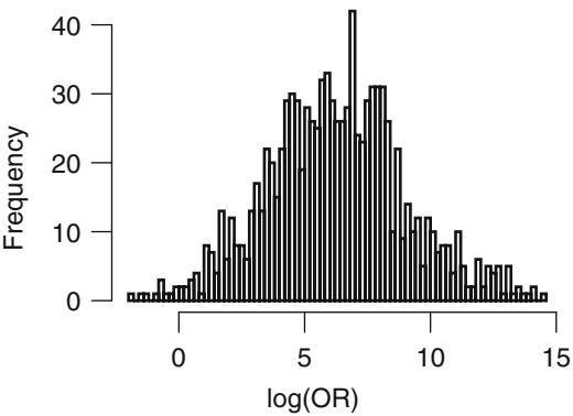

Fig. 9.4 Distribution of 1000 bootstrap x=1:5 log odds ratios

Figure 9.4 shows the distribution of log odds ratios.

Now consider confidence bands for the true log odds that y = 1, across a sequence of x values. The Predict function automatically calculates pointby-point bootstrap percentiles, basic bootstrap, or BCa203 confidence limits when the fit has passed through bootcov. Simultaneous Wald-based confidence intervals307 and Wald intervals substituting the bootstrap covariance matrix estimator are added to the plot when Predict calls the multcomp package (Figure 9.5).

x1s ← seq(0, 5, length =100)
pwald ← Predict(f, x1=x1s)
psand ← Predict( robcov (f), x1=x1s)
pbootcov ← Predict(b, x1=x1s , usebootcoef = FALSE )
pbootnp ← Predict(b, x1=x1s)
pbootbca ← Predict(b, x1=x1s , boot.type = ' bca ' )
pbootbas ← Predict(b, x1=x1s , boot.type = ' basic ' )
psimult ← Predict(b, x1=x1s , conf.type = ' simultaneous ' )

z ← rbind ( ' Boot percentile ' = pbootnp ,
           ' Robust sandwich ' = psand ,
           ' Boot BCa ' = pbootbca ,
           ' Boot covariance+ Wald ' = pbootcov ,
           Wald = pwald ,
           ' Boot basic ' = pbootbas ,
           Simultaneous = psimult)
z$class ← ifelse (z$.set. %in% c( ' Boot percentile ' , ' Boot bca ' ,
             ' Boot basic ' ), ' Other ' , ' Wald ' )
ggplot (z, groups =c( ' .set. ' , ' class ' ),
       conf= ' line ' , ylim=c(-1 , 9), legend.label = FALSE)

See Problems at chapter’s end for a worrisome investigation of bootstrap confidence interval coverage using simulation. It appears that when the model’s log odds distribution is not symmetric and includes very high or very low probabilities, neither the bootstrap percentile nor the bootstrap BCa intervals have good coverage, while the basic bootstrap and ordinary Wald intervals are fairly accuratef . It is difficult in general to know when to trust the bootstrap for logistic and perhaps other models when computing confidence intervals, and the simulation problem suggests that the basic bootstrap should be used more frequently. Similarly, the distribution of bootstrap effect estimates can be suspect. Asymmetry in this distribution does not imply that the true sampling distribution is asymmetric or that the percentile intervals are preferred.

9.8 Further Use of the Log Likelihood

9.8.1 Rating Two Models, Penalizing for Complexity

Suppose that from a single sample two competing models were developed. Let the respective −2 log likelihoods for these models be denoted by L¹ and L2, and let p¹ and p² denote the number of parameters estimated in each model. Suppose that L¹ < L2. It may be tempting to rate model one as the “best” fitting or “best” predicting model. That model may provide a better fit for the data at hand, but if it required many more parameters to be estimated, it may not be better “for the money.” If both models were applied to a new sample, model one’s overfitting of the original dataset may actually result in a worse fit on the new dataset.

^f Limited simulations using the conditional bootstrap and Firth’s penalized likelihood281 did not show significant improvement in confidence interval coverage.

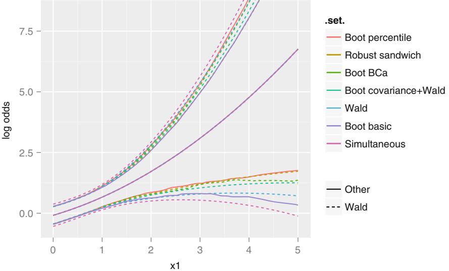
Fig. 9.5 Predicted log odds and confidence bands for seven types of confidence intervals. Seven categories are ordered top to bottom corresponding to order of lower confidence bands at x1=5. Dotted lines are for Wald–type methods that yield symmetric confidence intervals and assume normality of point estimators.

Akaike’s information criterion (AIC33, 359, 633) provides a method for penalizing the log likelihood achieved by a given model for its complexity to obtain a more unbiased assessment of the model’s worth. The penalty is to subtract the number of parameters estimated from the log likelihood, or equivalently to add twice the number of parameters to the −2 log likelihood. The penalized log likelihood is analogous to Mallows’ C^p in ordinary multiple regression. AIC would choose the model by comparing L¹ + 2p¹ to L² + 2p² ¹⁰ and picking the model with the lower value. We often use AIC in “adjusted χ²” form:

\[\text{AIC} = \text{LR} \propto \text{ $\chi$ }^2 - 2p. \tag{9.53}\]

Breiman [66, Section 1.3] and Chatfield [100, Section 4] discuss the fallacy of ¹¹ AIC and C^p for selecting from a series of non-prespecified models.

9.8.2 Testing Whether One Model Is Better than Another

One way to test whether one model (A) is better than another (B) is to embed both models in a more general model (A + B). Then a LR χ² test

can be done to test whether A is better than B by changing the hypothesis to test whether A adds predictive information to B (H⁰ : A + B>B) and whether B adds information to A (H⁰ : A+B>A). The approach of testing A>B via testing A+B>B and A+B>A is especially useful for selecting from competing predictors such as a multivariable model and a subjective assessor.131, 264, 395, 669

Note that LR χ² for H⁰ : A + B>B minus LR χ² for H⁰ : A + B>A equals LR χ² for H⁰ : A has no predictive information minus LR χ² for H⁰ : B has no predictive information,665 the difference in LR χ² for testing each model (set of variables) separately. This gives further support to the use of two separately computed Akaike’s information criteria for rating the two sets of variables. 12

See Section 9.8.4 for an example.

9.8.3 Unitless Index of Predictive Ability

The global likelihood ratio test for regression is useful for determining whether any predictor is associated with the response. If the sample is large enough, even weak associations can be “statistically significant.” Even though a likelihood ratio test does not shed light on a model’s predictive strength, the log likelihood (L.L.) can still be useful here. Consider the following L.L.s:

Best (lowest) possible −2 L.L.:

L^∗ = −2 L.L. for a hypothetical model that perfectly predicts the outcome.

−2 L.L. achieved: L = −2 L.L. for the fitted model.

Worst −2 L.L.:

^L⁰ ⁼ ⁻2 L.L. for a model that has no predictive information.

The last −2 L.L., for a “no information” model, is the −2 L.L. under the null hypothesis that all regression coefficients except for intercepts are zero. A “no information” model often contains only an intercept and some distributional parameters (a variance, for example). ¹³

The quantity ^L⁰ ⁻ ^L is LR, the log likelihood ratio statistic for testing the global null hypothesis that no predictors are related to the response. It is also the −2 log likelihood “explained” by the model. The best (lowest) −2 L.L. is L∗, so the amount of L.L. that is capable of being explained by the model is ^L⁰−L∗. The fraction of ⁻2 L.L. explained that was capable of being explained is

\[(L^0 - L)/(L^0 - L^\*) \quad = \quad LR/(L^0 - L^\*).\tag{9.54}\]

The fraction of log likelihood explained is analogous to R² in an ordinary linear model, although Korn and Simon365, 366 provide a much more precise notion.

Akaike’s information criterion can be used to penalize this measure of association for the number of parameters estimated (p, say) to transform this unitless measure of association into a quantity that is analogous to the adjusted R² or Mallows’ C^p in ordinary linear regression. We let R denote the square root of such a penalized fraction of log likelihood explained. R is defined by

\[R^2 = (LR - 2p)/(L\_0 - L^\*).\tag{9.55}\]

The R index can be used to assess how well the model compares with a “perfect” model, as well as to judge whether a more complex model has predictive strength that justifies its additional parameters. Had p been used in Equation 9.55 rather than 2p, R² is negative if the log likelihood explained is less than what one would expect by chance. R will be the square root of 1 − 2p/(L⁰ − L∗) if the model perfectly predicts the response. This upper limit will be near one if the sample size is large.

Partial R indexes can also be defined by substituting the −2 L.L. explained for a given factor in place of that for the entire model, LR. The “penalty factor” p becomes one. This index Rpartial is defined by

\[R\_{\text{partial}}^2 = (LR\_{\text{partial}} - 2)/(L\_0 - L^\*),\tag{9.56}\]

which is the (penalized) fraction of −2 log likelihood explained by the predictor. Here LRpartial is the log likelihood ratio statistic for testing whether the predictor is associated with the response, after adjustment for the other predictors. Since such likelihood ratio statistics are tedious to compute, the 1 d.f. Wald χ² can be substituted for the LR statistic (keeping in mind that difficulties with the Wald statistic can arise).

Liu and Dyer424 and Cox and Wermuth136 point out difficulties with the R² measure for binary logistic models. Cox and Snell135 and Magee432 used other analogies to derive other R² measures that may have better properties. For a sample of size n and a Wald statistic for testing overall association, they defined

\[\begin{split} R\_W^2 &= \frac{W}{n+W} \\ R\_{\rm LR}^2 &= 1 - \exp(-\rm LR/n) \\ &= 1 - \lambda^{2/n}, \end{split} \tag{9.57}\]

where λ is the null model likelihood divided by the fitted model likelihood. In the case of ordinary least squares with normality both of the above indexes are equal to the traditional R². R² LR is equivalent to Maddala’s index [431, Eq. 2.44]. Cragg and Uhler137 and Nagelkerke471 suggested dividing R² LR by its maximum attainable value

\[R\_{\text{max}}^2 = 1 - \exp(-L^0/n) \tag{9.58}\]

to derive R² ^N which ranges from 0 to 1. This is the form of the R² index we use throughout.

For penalizing for overfitting, see Verweij and van Houwelingen640 for an overfitting-corrected R² that uses a cross-validated likelihood. ¹⁴

9.8.4 Unitless Index of Adequacy of a Subset of Predictors

Log likelihoods are also useful for quantifying the predictive information contained in a subset of the predictors compared with the information contained in the entire set of predictors.264 Let LR again denote the ⁻2 log likelihood ratio statistic for testing the joint significance of the full set of predictors. Let LR^s denote the ⁻2 log likelihood ratio statistic for testing the importance of the subset of predictors of interest, excluding the other predictors from the model. A measure of adequacy of the subset for predicting the response is given by

\[A = LR^s/LR.\tag{9.59}\]

A is then the proportion of log likelihood explained by the subset with reference to the log likelihood explained by the entire set. When A = 1, the subset contains all the predictive information found in the whole set of predictors; that is, the subset is adequate by itself and the additional predictors contain no independent information. When A = 0, the subset contains no predictive information by itself.

Califf et al.89 used the A index to quantify the adequacy (with respect to prognosis) of two competing sets of predictors that each describe the extent of coronary artery disease. The response variable was time until cardiovascular death and the statistical model used was the Cox132 proportional hazards model. Some of their results are reproduced in Table 9.3. A chance-corrected ¹⁵ adequacy measure could be derived by squaring the ratio of the R-index for the subset to the R-index for the whole set. A formal test of superiority of X¹ = maximum % stenosis over X² = jeopardy score can be obtained by testing whether ^X¹ adds to ^X² (LR ^χ² = 57.⁵ ⁻ ⁴².6 = 14.9) and whether ^X² adds to ^X¹ (LR ^χ² = 57.5−51.8=5.7). ^X¹ adds more to ^X² (14.9) than X² adds to X¹ (5.7). The difference 14.9 − 5.7=9.2 equals the difference in single factor ^χ² (51.⁸ ⁻ ⁴².6)665.

Predictors Used	LR	χ2 Adequacy
Coronary jeopardy score	42.6	0.74
Maximum % stenosis in each artery	51.8	0.90
Combined	57.5	1.00

Table 9.3 Completing prognostic markers

9.9 Weighted Maximum Likelihood Estimation

It is commonly the case that data elements represent combinations of values that pertain to a set of individuals. This occurs, for example, when unique combinations of X and Y are determined from a massive dataset, along with the frequency of occurrence of each combination, for the purpose of reducing the size of the dataset to analyze. For the ith combination we have a case weight wⁱ that is a positive integer representing a frequency. Assuming that observations represented by combination i are independent, the likelihood needed to represent all wⁱ observations is computed simply by multiplying all of the likelihood elements (each having value Li), yielding a total likelihood contribution for combination i of L^wⁱ ⁱ or a log likelihood contribution of wⁱ log Li. To obtain a likelihood for the entire dataset one computes the product over all combinations. The total log likelihood is !wⁱ log Li. As an example, the weighted likelihood that would be used to fit a weighted logistic regression model is given by

\[L = \prod\_{i=1}^{n} P\_i^{w\_i Y\_i} (1 - P\_i)^{w\_i (1 - Y\_i)},\tag{9.60}\]

where there are n combinations, !ⁿ ⁱ=1 wⁱ > n, and Pⁱ is Prob[Yⁱ = 1|Xi] as dictated by the model. Note that in general the correct likelihood function cannot be obtained by weighting the data and using an unweighted likelihood.

By a small leap one can obtain weighted maximum likelihood estimates from the above method even if the weights do not represent frequencies or even integers, as long as the weights are non-negative. Non-frequency weights are commonly used in sample surveys to adjust estimates back to better represent a target population when some types of subjects have been oversampled from that population. Analysts should beware of possible losses in efficiency when obtaining weighted estimates in sample surveys.363, 364 Making the regression estimates conditional on sampling strata by including strata as covariables may be preferable to re-weighting the strata. If weighted estimates must be obtained, the weighted likelihood function is generally valid for obtaining properly weighted parameter estimates. However, the variance– covariance matrix obtained by inverting the information matrix from the weighted likelihood will not be correct in general. For one thing, the sum of the weights may be far from the number of subjects in the sample. A rough approximation to the variance–covariance matrix may be obtained by first multiplying each weight by n/!wⁱ and then computing the weighted information matrix, where n is the number of actual subjects in the sample.

9.10 Penalized Maximum Likelihood Estimation

Maximizing the log likelihood provides the best fit to the dataset at hand, but this can also result in fitting noise in the data. For example, a categorical predictor with 20 levels can produce extreme estimates for some of the 19 regression parameters, especially for the small cells (see Section 4.5). A shrinkage approach will often result in regression coefficient estimates that while biased are lower in mean squared error and hence are more likely to be close to the true unknown parameter values. Ridge regression is one approach to shrinkage, but a more general and better developed approach is penalized maximum likelihood estimation,237, 388, 639, 641 which is really a special case ¹⁷ of Bayesian modeling with a Gaussian prior. Letting L denote the usual likelihood function and λ be a penalty factor, we maximize the penalized log likelihood given by

\[\log L - \frac{1}{2}\lambda \sum\_{i=1}^{p} (s\_i \beta\_i)^2,\tag{9.61}\]

where s1, s2,…,s^p are scale factors chosen to make siβⁱ unitless. Most authors standardize the data first and do not have scale factors in the equation, but Equation 9.61 has the advantage of allowing estimation of β on the original scale of the data. The usual methods (e.g., Newton–Raphson) are used to maximize 9.61.

The choice of the scaling constants has received far too little attention in the ridge regression and penalized MLE literature. It is common to use the ¹⁸ standard deviation of each column of the design matrix to scale the corresponding parameter. For models containing nothing but continuous variables that enter the regression linearly, this is usually a reasonable approach. For continuous variables represented with multiple terms (one of which is linear), it is not always reasonable to scale each nonlinear term with its own standard deviation. For dummy variables, scaling using the standard deviation (&d(1 ⁻ ^d), where ^d is the mean of the dummy variable, i.e., the fraction of observations in that cell) is problematic since this will result in high prevalance cells getting more shrinkage than low prevalence ones because the high prevalence cells will dominate the penalty function.

An advantage of the formulation in Equation 9.61 is that one can assign scale constants of zero for parameters for which no shrinkage is desired.237, 639 For example, one may have prior beliefs that a linear additive model will fit the data. In that case, nonlinear and non-additive terms may be penalized.

For a categorical predictor having c levels, users of ridge regression often do not recognize that the amount of shrinkage and the predicted values from the fitted model depend on how the design matrix is coded. For example, one will get different predictions depending on which cell is chosen as the reference cell when constructing dummy variables. The setup in Equation 9.61 has the same problem. For example, if for a three-category factor we use category 1 as the reference cell and have parameters β² and β3, the unscaled penalty function is β² ² + β² ³. If category 3 were used as the reference cell instead, the penalty would be β² ³ + (β² ⁻ ^β3)2. To get around this problem, Verweij and van Houwelingen639 proposed using the penalty function !^c ⁱ (βⁱ ⁻ ^β)2, where β is the mean of all c βs. This causes shrinkage of all parameters toward the mean parameter value. Letting the first category be the reference cell, we use c − 1 dummy variables and define β¹ ≡ 0. For the case c = 3 the sum of squares is 2[β² ² + β² ³ ⁻ ^β2β3]/3. For ^c = 2 the penalty is ^β² ² /2. If no scale constant is used, this is the same as scaling ^β² with ^√² ^× the standard deviation of a binary dummy variable with prevalance of 0.5.

The sum of squares can be written in matrix form as [β2,…, βc] ′ (A − B)[β2,…, βc], where A is a c − 1 × c − 1 identity matrix and B is ^a ^c ⁻ ¹ ^× ^c ⁻ 1 matrix all of whose elements are ¹ ^c ¹⁹ .

For general penalty functions such as that just described, the penalized log likelihood can be generalized to

\[ \log L - \frac{1}{2}\lambda\beta'P\beta. \tag{9.62} \]

For purposes of using the Newton–Raphson procedure, the first derivative of the penalty function with respect to β is −λPβ, and the negative of the second derivative is λP.

²⁰ Another problem in penalized estimation is how the choice of λ is made. Many authors use cross-validation. A limited number of simulation studies in binary logistic regression modeling has shown that for each λ being considered, at least 10-fold cross-validation must be done so as to obtain a reasonable estimate of predictive accuracy. Even then, a smoother207 (“super smoother”) must be used on the (λ, accuracy) pairs to allow location of the optimum value unless one is careful in choosing the initial sub-samples and uses these same splits throughout. Simulation studies have shown that a modified AIC is not only much quicker to compute (since it requires no cross-²¹ validation) but performs better at finding a good value of λ (see below).

For a given λ, the effective number of parameters being estimated is reduced because of shrinkage. Gray [237, Eq. 2.9] and others estimate the effective degrees of freedom by computing the expected value of a global Wald statistic for testing association, when the null hypothesis of no association is true. The d.f. is equal to

\[\text{trace}[I(\hat{\beta}^P)V(\hat{\beta}^P)],\tag{9.63}\]

where βˆ^P is the penalized MLE (the parameters that maximize Equation 9.61), I is the information matrix computed from ignoring the penalty function, and V is the covariance matrix computed by inverting the information matrix that included the second derivatives with respect to β in the penalty function. 22

Gray [237, Eq. 2.6] states that a better estimate of the variance–covariance matrix for βˆ^P than V (βˆ^P ) is

\[V^\* = V(\hat{\beta}^P)I(\hat{\beta}^P)V(\hat{\beta}^P). \tag{9.64}\]

Therneau (personal communication, 2000) has found in a limited number of simulation studies that V ∗ underestimates the true variances, and that a better estimate of the variance–covariance matrix is simply V (βˆ^P ), assuming that the model is correctly specified. This is the covariance matrix used by default in the rms package (the user can request that the sandwich estimator be used instead) and is in fact the one Gray used for Wald tests.

Penalization will bias estimates of β, so hypothesis tests and confidence intervals using βˆ^P may not have a simple interpretation. The same problem arises in score and likelihood ratio tests. So far, penalization is better understood in pure prediction mode unless Bayesian methods are used.

Equation 9.63 can be used to derive a modified AIC (see [639, Eq. 6] and [641, Eq. 7]) on the model χ² scale:

\[\text{LR} \propto \chi^2 - 2 \times \text{ effective d.f.},\tag{9.65}\]

where LR χ² is the likelihood ratio χ² for the penalized model, but ignoring the penalty function. If a variety of λ are tried and one plots the (λ, AIC) pairs, the λ that maximizes AIC will often be a good choice, that is, it is likely to be near the value of λ that maximizes predictive accuracy on a future datasetg.

Note that if one does penalized maximum likelihood estimation where a set of variables being penalized has a negative value for the unpenalized ^χ²−² ^× d.f., the value of λ that will optimize the overall model AIC will be ∞.

As an example, consider some simulated data (n = 100) with one predictor in which the true model is Y = X¹ + ϵ, where ϵ has a standard normal distribution and so does X1. We use a series of penalties (found by trial and error) that give rise to sensible effective d.f., and fit penalized restricted cubic spline functions with five knots. We penalize two ways: all terms in the model including the coefficient of X1, which in reality needs no penalty; and only the nonlinear terms. The following R program, in conjunction with the rms package, does the job.

^g Several examples from simulated datasets have shown that using BIC to choose a penalty results in far too much shrinkage.

set.seed (191)
x1 ← rnorm (100)
y ← x1 + rnorm (100)
pens ← df ← aic ← c(0,.07 ,.5 ,2,6,15,60)
all ← nl ← list ()
for(penalize in 1:2) {
  for(i in 1:length (pens )) {
    f ← ols(y ∼ rcs(x1 ,5), penalty=
              list(simple =if( penalize ==1) pens[i] else 0,
                   nonlinear= pens[i]))
    df[i] ← f$stats[ ' d.f. ' ]
    aic[i] ← AIC(f)
    nam ← paste (if( penalize == 1) ' all ' else ' nl ' ,
                   ' penalty: ' , pens[i], sep= ' ' )
    nam ← as.character ( pens[i])
    p ← Predict(f, x1=seq(-2.5 , 2.5 , length =100),
                  conf.int= FALSE)
    if(penalize == 1) all[[nam]] ← p else nl[[nam]] ← p
  }
  print (rbind (df=df , aic=aic))
}

[,1] [,2] [,3] [,4] [,5] [,6]
df 4.0000 3.213591 2.706069 2.30273 2.029282 1.822758
aic 270.6653 269.154045 268.222855 267.56594 267.288988 267.552915
        [,7]
df 1.513609
aic 270.805033
      [,1] [,2] [,3] [,4] [,5] [,6]
df 4.0000 3.219149 2.728126 2.344807 2.109741 1.960863
aic 270.6653 269.167108 268.287933 267.718681 267.441197 267.347475
        [,7]
df 1.684421
aic 267.892073

all ← do.call( ' rbind ' , all); all$type ← ' Penalize All '
nl ← do.call( ' rbind ' , nl) ; nl$type ← ' Penalize Nonlinear '
both ← as.data.frame(rbind.data.frame(all , nl))
both$Penalty ← both$.set.
ggplot (both , aes(x=x1, y=yhat , color=Penalty )) + geom_line () +
  geom_abline (col=gray(.7)) + facet_grid (∼ type)
# Figure 9.6

The left panel in Figure 9.6 corresponds to penalty = list(simple=a, nonlinear=a) in the R program, meaning that all parameters except the intercept are shrunk by the same amount a (this would be more appropriate had there been multiple predictors). As effective d.f. get smaller (penalty factor gets larger), the regression fits get flatter (too flat for the largest penalties) and confidence bands get narrower. The right graph corresponds to penalty=list(simple=0, nonlinear=a), causing only the cubic spline terms that are nonlinear in X¹ to be shrunk. As the amount of shrinkage increases (d.f. lowered), the fits become more linear and closer to the true regression line (longer dotted line). ²³ Again, confidence intervals become smaller.

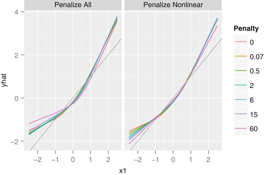
Fig. 9.6 Penalized least squares estimates for an unnecessary five-knot restricted cubic spline function. In the left graph all parameters (except the intercept) are penalized. The effective d.f. are 4, 3.21, 2.71, 2.30, 2.03, 1.82, and 1.51. In the right graph, only parameters associated with nonlinear functions of X¹ are penalized. The effective d.f. are 4, 3.22, 2.73, 2.34, 2.11, 1.96, and 1.68.

9.11 Further Reading

1 Boos60 has some nice generalizations of the score test. Morgan et al.464 show how score test χ² statistics may negative unless the expected information matrix is used.
2 See Marubini and Valsecchi [444, pp. 164–169] for an excellent description of the relationship between the three types of test statistics.
3 References [115,507] have good descriptions of methods used to maximize log L. 4 As Long and Ervin426 argue, for small sample sizes, the usual Huber–White covariance estimator should not be used because there the residuals do not have constant variance even under homoscedasticity. They showed that a simple correction due to Efron and others can result in substantially better estimates. Lin and Wei,410 Binder,55 and Lin407 have applied the Huber estimator to the Cox132 survival model. Freedman206 questioned the use of sandwich estimators because they are often used to obtain the right variances on the wrong parameters when the model doesn’t fit. He also has some excellent background information.
5 Feng et al.188 showed that in the case of cluster correlations arising from repeated measurement data with Gaussian errors, the cluster bootstrap performs excellently even when the number of observations per cluster is large and the number of subjects is small. Xiao and Abrahamowicz676 compared the cluster bootstrap with a two-stage cluster bootstrap in the context of the Cox model.
6 Graubard and Korn235 and Fitzmaurice195 describe the kinds of situations in which the working independence model can be trusted.
7 Minkin,460 Alho,11 Doganaksoy and Schmee,160 and Meeker and Escobar452 discuss the need for LR and score-based confidence intervals. Alho found that score-based intervals are usually more tedious to compute, and provided useful algorithms for the computation of either type of interval (see also [452] and [444, p. 167]). Score and LR intervals require iterative computations and have to deal with the fact that when one parameter is changed (e.g., bⁱ is restricted to be zero), all other parameter estimates change. DiCiccio and Efron157 provide a method for very accurate confidence intervals for exponential families that requires a modest amount of additional computation. Venzon and Moolgavkar provide an efficient general method for computing LR-based intervals.636 Brazzale and Davison65 developed some promising and feasible ways to make unconditional likelihood-based inferences more accurate in small samples.
8 Carpenter and Bithell92 have an excellent overview of several variations on the bootstrap for obtaining confidence limits.
9 Tibshirani and Knight610 developed an easy to program approach for deriving simultaneous confidence sets that is likely to be useful for getting simultaneous confidence regions for the entire vector of model parameters, for population values for an entire sequence of predictor values, and for a set of regression effects (e.g., interquartile-range odds ratios for age for both sexes). The basic idea is that during the, say, 1000 bootstrap repetitions one stores the −2 log likelihood for each model fit, being careful to compute the likelihood at the current bootstrap parameter estimates but with respect to the original data matrix, not the bootstrap sample of the data matrix. To obtain an approximate simultaneous 0.95 confidence set one computes the 0.95 quantile of the −2 log likelihood values and determines which vectors of parameter estimates correspond to −2 log likelihoods that are at least as small as the 0.95 quantile of all −2 log likelihoods. Once the qualifying parameter estimates are found, the quantities of interest are computed from those parameter estimates and an outer envelope of those quantities is found. Computations are facilitated with the rms package confplot function.
10 van Houwelingen and le Cessie [633, Eq. 52] showed, consistent with AIC, that the average optimism in a mean logarithmic (minus log likelihood) quality score for logistic models is p/n.
11 Schwarz560 derived a different penalty using large-sample Bayesian properties of competing models. His Bayesian Information Criterion (BIC) chooses the model having the lowest value of L + 1/2p log n or the highest value of LR ^χ² ⁻ ^p log ⁿ. Kass and Raftery have done several studies of BIC.337 Smith and Spiegelhalter576 and Laud and Ibrahim377 discussed other useful generalizations of likelihood penalties. Zheng and Loh685 studied several penalty measures, and found that AIC does not penalize enough for overfitting in the ordinary regression case. Kass and Raftery [337, p. 790] provide a nice review of this topic, stating that “AIC picks the correct model asymptotically if the complexity of the true model grows with sample size” and that “AIC selects models that are too big even when the sample size is large.” But they also cite other papers that show the existence of cases where AIC can work better than BIC. According to Buckland et al.,80 BIC “assumes that a true model exists and is low-dimensional.”

Hurvich and Tsai314,315 made an improvement in AIC that resulted in much better model selection for small n. They defined the corrected AIC as

\[\text{AIC}\_C = \text{LR } \chi^2 - 2p[1 + \frac{p+1}{n-p-1}].\tag{9.66}\]

In [314] they contrast asymptotically efficient model selection with AIC when the true model has infinitely many parameters with improvements using other indexes such as AIC^C when the model is finite.

One difficulty in applying the Schwarz, AICC, and related criteria is that with censored or binary responses it is not clear that the actual sample size n should be used in the formula.

12 Goldstein,222 Willan et al.,669 and Royston and Thompson534 have nice discussions on comparing non-nested regression models. Schemper’s method549 is useful for testing whether a set of variables provides significantly greater information (using an R² measure) than another set of variables.
13 van Houwelingen and le Cessie [633, Eq. 22] recommended using L/2 (also called the Kullback–Leibler error rate) as a quality index.
14 Schemper549 provides a bootstrap technique for testing for significant differences between correlated R² measures. Mittlb¨ock and Schemper,461 Schemper and Stare,554 Korn and Simon,365,366 Menard,454 and Zheng and Agresti684 have excellent discussions about the pros and cons of various indexes of the predictive value of a model.
15 Al-Radi et al.10 presented another analysis comparing competing predictors using the adequacy index and a receiver operating characteristic curve area approach based on a test for whether one predictor has a higher probability of being “more concordant” than another.
16 [55,97,409] provide good variance–covariance estimators from a weighted maximum likelihood analysis.
17 Huang and Harrington310 developed penalized partial likelihood estimates for Cox models and provided useful background information and theoretical results about improvements in mean squared errors of regression estimates. They used a bootstrap error estimate for selection of the penalty parameter.
18 Sardy538 proposes that the square roots of the diagonals of the inverse of the covariance matrix for the predictors be used for scaling rather than the standard deviations.
19 Park and Hastie483 and articles referenced therein describe how quadratic penalized logistic regression automatically sets coefficient estimates for empty cells to zero and forces the sum of k coefficients for a k-level categorical predictor to equal zero.
20 Greenland241 has a nice discussion of the relationship between penalized maximum likelihood estimation and mixed effects models. He cautions against estimating the shrinkage parameter.
21 See310 for a bootstrap approach to selection of λ.
22 Verweij and van Houwelingen [639, Eq. 4] derived another expression for d.f., but it requires more computation and did not perform any better than Equation 9.63 in choosing λ in several examples tested.
23 See van Houwelingen and Thorogood631 for an approximate empirical Bayes approach to shrinkage. See Tibshirani608 for the use of a non-smooth penalty function that results in variable selection as well as shrinkage (see Section 4.3). Verweij and van Houwelingen640 used a “cross-validated likelihood” based on leave-out-one estimates to penalize for overfitting. Wang and Taylor652 presented some methods for carrying out hypothesis tests and computing confidence limits under penalization. Moons et al.462 presented a case study of penalized estimation and discussed the advantages of penalization.

Variables in Model	χ2 LR
age	100
sex	108
age, sex	111
age2	60
age, age2	102
age, age2, sex	115

Table 9.4 Likelihood ratio global test statistics

9.12 Problems

A sample of size 100 from a normal distribution with unknown mean and standard deviation (µ and σ) yielded the following log likelihood values when computed at two values of µ.

\[\begin{aligned} \log L(\mu = 10, \sigma = 5) &= -800 \\ \log L(\mu = 20, \sigma = 5) &= -820. \end{aligned}\]

What do you know about µ? What do you know about Y ?

1. Several regression models were considered for predicting a response. LR χ² (corrected for the intercept) for models containing various combinations of variables are found in Table 9.4. Compute all possible meaningful LR χ². For each, state the d.f. and an approximate P-value. State which LR χ² involving only one variable is not very meaningful.
1. For each problem below, rank Wald, score, and LR statistics by overall statistical properties and then by computational convenience.
- 1. A forward stepwise variable selection (to be later accounted for with the bootstrap) is desired to determine a concise model that contains most of the independent information in all potential predictors.
- 1. A test of independent association of each variable in a given model (each variable adjusted for the effects of all other variables in the given model) is to be obtained.
- 1. A model that contains only additive effects is fitted. A large number of potential interaction terms are to be tested using a global (multiple d.f.) test.
1. Consider a univariate saturated model in 3 treatments (A, B, C) that is quadratic in age. Write out the model with all the βs, and write in detail the contrast for comparing treatment B with treatment C for 30 year olds. Sketch out the same contrast using the “difference in predictions” approach without simplification.
1. Simulate a binary logistic model for n = 300 with an average fraction of events somewhere between 0.15 and 0.3. Use 5 continuous covariates and assume the model is everywhere linear. Fit an unpenalized model, then solve for the optimum quadratic penalty λ. Relate the resulting effective d.f. to the 15:1 rule of thumb, and compute the heuristic shrinkage coefficient ˆγ for the unpenalized model and for the optimally penalized model, inserting the effective d.f. for the number of non-intercept parameters in the model.
1. For a similar setup as the binary logistic model simulation in Section 9.7, do a Monte Carlo simulation to determine the coverage probabilities for ordinary Wald and for three types of bootstrap confidence intervals for the true x=5 to x=1 log odds ratio. In addition, consider the Wald-type confidence interval arising from the sandwich covariance estimator. Estimate the non-coverage probabilities in both tails. Use a sample size n = 200 with the single predictor x¹ having a standard log-normal distribution, and the true model being logit(Y = 1) = 1 + x1/2. Determine whether increasing the sample size relieves any problem you observed. Some R code for this simulation is on the web site.

Frank E. Harrell, Jr.

Regression Modeling Strategies

Springer Series in Statistics

Regression Modeling Strategies

Preface

Acknowledgments

Contents

Typographical Conventions

Chapter 1 Introduction

1.1 Hypothesis Testing, Estimation, and Prediction

1.2 Examples of Uses of Predictive Multivariable Modeling

1.3 Prediction vs. Classification

1.4 Planning for Modeling

1.4.1 Emphasizing Continuous Variables

1.5 Choice of the Model

1.6 Further Reading 11

1.6 Further Reading

Chapter 2 General Aspects of Fitting Regression Models

2.1 Notation for Multivariable Regression Models

2.2 Model Formulations

2.3 Interpreting Model Parameters

2.3.1 Nominal Predictors

2.3.2 Interactions

2.3.3 Example: Inference for a Simple Model

2.4 Relaxing Linearity Assumption for Continuous Predictors

2.4.1 Avoiding Categorization

2.4.2 Simple Nonlinear Terms

2.4.3 Splines for Estimating Shape of Regression Function and Determining Predictor Transformations

2.4.4 Cubic Spline Functions

2.4.5 Restricted Cubic Splines

2.4.6 Choosing Number and Position of Knots

2.4.7 Nonparametric Regression

2.4.8 Advantages of Regression Splines over Other Methods

2.5 Recursive Partitioning: Tree-Based Models

2.6 Multiple Degree of Freedom Tests of Association

2.7 Assessment of Model Fit

2.7.1 Regression Assumptions

2.7.2 Modeling and Testing Complex Interactions

2.7.3 Fitting Ordinal Predictors

2.7.4 Distributional Assumptions

2.8 Further Reading

2.8 Further Reading 41

2.9 Problems

2.9 Problems 43

Chapter 3 Missing Data

3.1 Types of Missing Data

Informative missing (IM)

3.2 Prelude to Modeling

3.3 Missing Values for Different Types of Response Variables

3.4 Problems with Simple Alternatives to Imputation

3.5 Strategies for Developing an Imputation Model

3.6 Single Conditional Mean Imputation

3.7 Predictive Mean Matching

3.8 Multiple Imputation

3.8.1 The aregImpute and Other Chained Equations Approaches

3.9 Diagnostics

3.10 Summary and Rough Guidelines

3.11 Further Reading

3.12 Problems

Chapter 4 Multivariable Modeling Strategies

4.1 Prespecification of Predictor Complexity Without Later Simplification

4.2 Checking Assumptions of Multiple Predictors Simultaneously

4.3 Variable Selection

4.3 Variable Selection 69

4.4 Sample Size, Overfitting, and Limits on Number of Predictors

4.5 Shrinkage

4.6 Collinearity

4.7 Data Reduction

4.7.1 Redundancy Analysis

4.7.2 Variable Clustering

4.7.3 Transformation and Scaling Variables Without Using Y

4.7.4 Simultaneous Transformation and Imputation

4.7 Data Reduction 85

4.7.5 Simple Scoring of Variable Clusters

4.7.6 Simplifying Cluster Scores

4.7.7 How Much Data Reduction Is Necessary?

4.8 Other Approaches to Predictive Modeling

4.9 Overly Influential Observations

4.10 Comparing Two Models

4.11 Improving the Practice of Multivariable Prediction