The Elements of Statistical Learning

Chapter 10 ~ 18

This is page 337 Printer: Opaque this

10 Boosting and Additive Trees

10.1 Boosting Methods

Boosting is one of the most powerful learning ideas introduced in the last twenty years. It was originally designed for classification problems, but as will be seen in this chapter, it can profitably be extended to regression as well. The motivation for boosting was a procedure that combines the outputs of many “weak” classifiers to produce a powerful “committee.” From this perspective boosting bears a resemblance to bagging and other committee-based approaches (Section 8.8). However we shall see that the connection is at best superficial and that boosting is fundamentally different.

We begin by describing the most popular boosting algorithm due to Freund and Schapire (1997) called “AdaBoost.M1.” Consider a two-class problem, with the output variable coded as Y ∈ {−1, 1}. Given a vector of predictor variables X, a classifier G(X) produces a prediction taking one of the two values {−1, 1}. The error rate on the training sample is

\[\overline{\text{err}} = \frac{1}{N} \sum\_{i=1}^{N} I(y\_i \neq G(x\_i)),\]

and the expected error rate on future predictions is EXY I(Y ̸= G(X)).

A weak classifier is one whose error rate is only slightly better than random guessing. The purpose of boosting is to sequentially apply the weak classification algorithm to repeatedly modified versions of the data, thereby producing a sequence of weak classifiers Gm(x), m = 1, 2,…,M.

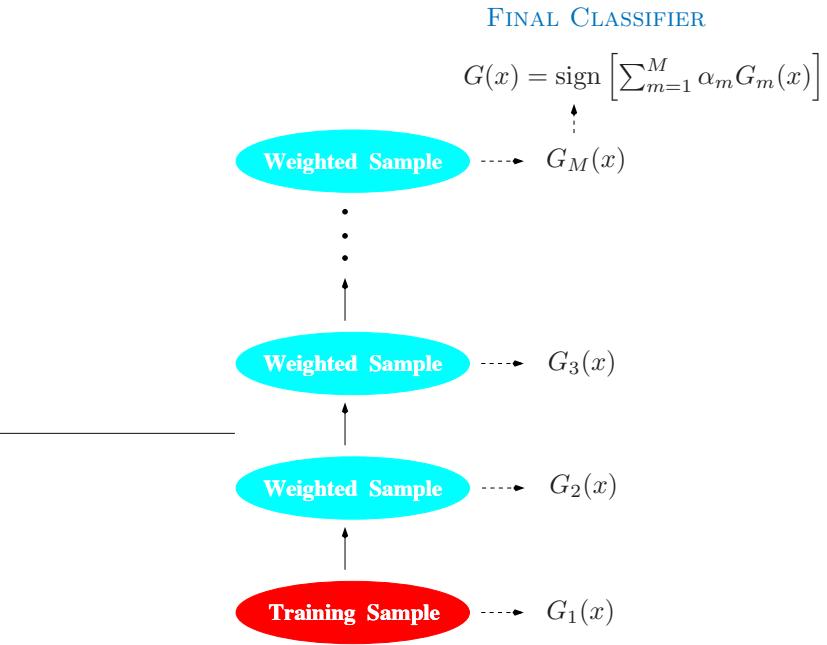
FIGURE 10.1. Schematic of AdaBoost. Classifiers are trained on weighted versions of the dataset, and then combined to produce a final prediction.

The predictions from all of them are then combined through a weighted majority vote to produce the final prediction:

\[G(x) = \text{sign}\left(\sum\_{m=1}^{M} \alpha\_m G\_m(x)\right). \tag{10.1}\]

Here α1, α2,…, α^M are computed by the boosting algorithm, and weight the contribution of each respective Gm(x). Their effect is to give higher influence to the more accurate classifiers in the sequence. Figure 10.1 shows a schematic of the AdaBoost procedure.

The data modifications at each boosting step consist of applying weights w1, w2,…,w^N to each of the training observations (xi, yi), i = 1, 2,…,N. Initially all of the weights are set to wⁱ = 1/N, so that the first step simply trains the classifier on the data in the usual manner. For each successive iteration m = 2, 3,…,M the observation weights are individually modified and the classification algorithm is reapplied to the weighted observations. At step m, those observations that were misclassified by the classifier Gm−1(x) induced at the previous step have their weights increased, whereas the weights are decreased for those that were classified correctly. Thus as iterations proceed, observations that are difficult to classify correctly receive ever-increasing influence. Each successive classifier is thereby forced Algorithm 10.1 AdaBoost.M1.

• 1. Initialize the observation weights wⁱ = 1/N, i = 1, 2,…,N.
• 2. For m = 1 to M:
  • 1. Fit a classifier Gm(x) to the training data using weights wi.
  • 2. Compute

\[\text{err}\_m = \frac{\sum\_{i=1}^N w\_i I(y\_i \neq G\_m(x\_i))}{\sum\_{i=1}^N w\_i}.\]

• 3. Compute α^m = log((1 − errm)/errm).
• 4. Set wⁱ ← wⁱ · exp[α^m · I(yⁱ ̸= Gm(xi))], i = 1, 2,…,N.

\[3.\text{ Output }G(x) = \text{sign}\left[\sum\_{m=1}^{M} \alpha\_m G\_m(x)\right].\]

to concentrate on those training observations that are missed by previous ones in the sequence.

Algorithm 10.1 shows the details of the AdaBoost.M1 algorithm. The current classifier Gm(x) is induced on the weighted observations at line 2a. The resulting weighted error rate is computed at line 2b. Line 2c calculates the weight α^m given to Gm(x) in producing the final classifier G(x) (line 3). The individual weights of each of the observations are updated for the next iteration at line 2d. Observations misclassified by Gm(x) have their weights scaled by a factor exp(αm), increasing their relative influence for inducing the next classifier Gm+1(x) in the sequence.

The AdaBoost.M1 algorithm is known as “Discrete AdaBoost” in Friedman et al. (2000), because the base classifier Gm(x) returns a discrete class label. If the base classifier instead returns a real-valued prediction (e.g., a probability mapped to the interval [−1, 1]), AdaBoost can be modified appropriately (see “Real AdaBoost” in Friedman et al. (2000)).

The power of AdaBoost to dramatically increase the performance of even a very weak classifier is illustrated in Figure 10.2. The features X1,…,X¹⁰ are standard independent Gaussian, and the deterministic target Y is defined by

\[Y = \begin{cases} 1 & \text{if } \sum\_{j=1}^{10} X\_j^2 > \chi\_{10}^2(0.5), \\ -1 & \text{otherwise.} \end{cases} \tag{10.2}\]

Here χ^{2 10}(0.5) = 9.34 is the median of a chi-squared random variable with 10 degrees of freedom (sum of squares of 10 standard Gaussians). There are 2000 training cases, with approximately 1000 cases in each class, and 10,000 test observations. Here the weak classifier is just a “stump”: a two terminalnode classification tree. Applying this classifier alone to the training data set yields a very poor test set error rate of 45.8%, compared to 50% for

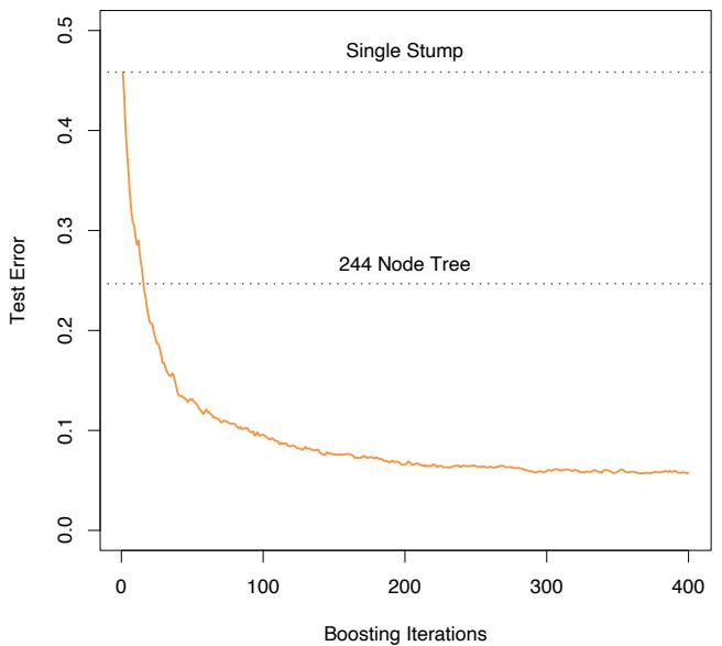
FIGURE 10.2. Simulated data (10.2): test error rate for boosting with stumps, as a function of the number of iterations. Also shown are the test error rate for a single stump, and a 244-node classification tree.

random guessing. However, as boosting iterations proceed the error rate steadily decreases, reaching 5.8% after 400 iterations. Thus, boosting this simple very weak classifier reduces its prediction error rate by almost a factor of four. It also outperforms a single large classification tree (error rate 24.7%). Since its introduction, much has been written to explain the success of AdaBoost in producing accurate classifiers. Most of this work has centered on using classification trees as the “base learner” G(x), where improvements are often most dramatic. In fact, Breiman (NIPS Workshop, 1996) referred to AdaBoost with trees as the “best off-the-shelf classifier in the world” (see also Breiman (1998)). This is especially the case for datamining applications, as discussed more fully in Section 10.7 later in this chapter.

10.1.1 Outline of This Chapter

Here is an outline of the developments in this chapter:

• We show that AdaBoost fits an additive model in a base learner, optimizing a novel exponential loss function. This loss function is very similar to the (negative) binomial log-likelihood (Sections 10.2– 10.4).

• The population minimizer of the exponential loss function is shown to be the log-odds of the class probabilities (Section 10.5).
• We describe loss functions for regression and classification that are more robust than squared error or exponential loss (Section 10.6).
• It is argued that decision trees are an ideal base learner for data mining applications of boosting (Sections 10.7 and 10.9).
• We develop a class of gradient boosted models (GBMs), for boosting trees with any loss function (Section 10.10).
• The importance of “slow learning” is emphasized, and implemented by shrinkage of each new term that enters the model (Section 10.12), as well as randomization (Section 10.12.2).
• Tools for interpretation of the fitted model are described (Section 10.13).

10.2 Boosting Fits an Additive Model

The success of boosting is really not very mysterious. The key lies in expression (10.1). Boosting is a way of fitting an additive expansion in a set of elementary “basis” functions. Here the basis functions are the individual classifiers Gm(x) ∈ {−1, 1}. More generally, basis function expansions take the form

\[f(x) = \sum\_{m=1}^{M} \beta\_m b(x; \gamma\_m),\tag{10.3}\]

where βm, m = 1, 2,…,M are the expansion coefficients, and b(x; γ) ∈ IR are usually simple functions of the multivariate argument x, characterized by a set of parameters γ. We discuss basis expansions in some detail in Chapter 5.

Additive expansions like this are at the heart of many of the learning techniques covered in this book:

• In single-hidden-layer neural networks (Chapter 11), b(x; γ) = σ(γ⁰ + γT ¹ x), where σ(t)=1/(1+e−^t ) is the sigmoid function, and γ parameterizes a linear combination of the input variables.
• In signal processing, wavelets (Section 5.9.1) are a popular choice with γ parameterizing the location and scale shifts of a “mother” wavelet.
• Multivariate adaptive regression splines (Section 9.4) uses truncatedpower spline basis functions where γ parameterizes the variables and values for the knots.

Algorithm 10.2 Forward Stagewise Additive Modeling.

• 1. Initialize f0(x) = 0.
• 2. For m = 1 to M:
  • 1. Compute

\[(\beta\_m, \gamma\_m) = \arg\min\_{\beta, \gamma} \sum\_{i=1}^N L(y\_i, f\_{m-1}(x\_i) + \beta b(x\_i; \gamma)).\]

\[\text{(b) Set } f\_m(x) = f\_{m-1}(x) + \beta\_m b(x; \gamma\_m).\]

• For trees, γ parameterizes the split variables and split points at the internal nodes, and the predictions at the terminal nodes.

Typically these models are fit by minimizing a loss function averaged over the training data, such as the squared-error or a likelihood-based loss function,

\[\min\_{\{\beta\_m, \gamma\_m\}\_1^M} \sum\_{i=1}^N L\left(y\_i, \sum\_{m=1}^M \beta\_m b(x\_i; \gamma\_m)\right). \tag{10.4}\]

For many loss functions L(y, f(x)) and/or basis functions b(x; γ), this requires computationally intensive numerical optimization techniques. However, a simple alternative often can be found when it is feasible to rapidly solve the subproblem of fitting just a single basis function,

\[\min\_{\beta, \gamma} \sum\_{i=1}^{N} L\left(y\_i, \beta b(x\_i; \gamma)\right). \tag{10.5}\]

10.3 Forward Stagewise Additive Modeling

Forward stagewise modeling approximates the solution to (10.4) by sequentially adding new basis functions to the expansion without adjusting the parameters and coefficients of those that have already been added. This is outlined in Algorithm 10.2. At each iteration m, one solves for the optimal basis function b(x; γm) and corresponding coefficient β^m to add to the current expansion fm−1(x). This produces fm(x), and the process is repeated. Previously added terms are not modified.

For squared-error loss

\[L(y, f(x)) = (y - f(x))^2,\tag{10.6}\]

one has

\[\begin{split} L(y\_i, f\_{m-1}(x\_i) + \beta b(x\_i; \gamma)) &= (y\_i - f\_{m-1}(x\_i) - \beta b(x\_i; \gamma))^2 \\ &= (r\_{im} - \beta b(x\_i; \gamma))^2, \end{split} \tag{10.7}\]

where rim = yⁱ − fm−1(xi) is simply the residual of the current model on the ith observation. Thus, for squared-error loss, the term βmb(x; γm) that best fits the current residuals is added to the expansion at each step. This idea is the basis for “least squares” regression boosting discussed in Section 10.10.2. However, as we show near the end of the next section, squared-error loss is generally not a good choice for classification; hence the need to consider other loss criteria.

10.4 Exponential Loss and AdaBoost

We now show that AdaBoost.M1 (Algorithm 10.1) is equivalent to forward stagewise additive modeling (Algorithm 10.2) using the loss function

\[L(y, f(x)) = \exp(-y \, f(x)).\tag{10.8}\]

The appropriateness of this criterion is addressed in the next section.

For AdaBoost the basis functions are the individual classifiers Gm(x) ∈ {−1, 1}. Using the exponential loss function, one must solve

\[(\beta\_m, G\_m) = \arg\min\_{\beta, G} \sum\_{i=1}^N \exp[-y\_i(f\_{m-1}(x\_i) + \beta \, G(x\_i))]\]

for the classifier G^m and corresponding coefficient β^m to be added at each step. This can be expressed as

\[\left(\beta\_m, G\_m\right) = \arg\min\_{\beta, G} \sum\_{i=1}^N w\_i^{(m)} \exp(-\beta \, y\_i \, G(x\_i))\tag{10.9}\]

with w(m) ⁱ = exp(−y^{i f}m−1(xi)). Since each ^w(m) ⁱ depends neither on β nor G(x), it can be regarded as a weight that is applied to each observation. This weight depends on fm−1(xi), and so the individual weight values change with each iteration m.

The solution to (10.9) can be obtained in two steps. First, for any value of β > 0, the solution to (10.9) for Gm(x) is

\[G\_m = \arg\min\_G \sum\_{i=1}^N w\_i^{(m)} I(y\_i \neq G(x\_i)),\tag{10.10}\]

344 10. Boosting and Additive Trees

which is the classifier that minimizes the weighted error rate in predicting y. This can be easily seen by expressing the criterion in (10.9) as

\[e^{-\beta} \cdot \sum\_{y\_i = G(x\_i)} w\_i^{(m)} + e^{\beta} \cdot \sum\_{y\_i \neq G(x\_i)} w\_i^{(m)},\]

which in turn can be written as

\[I\left(e^{\beta} - e^{-\beta}\right) \cdot \sum\_{i=1}^{N} w\_i^{\{m\}} I(y\_i \neq G(x\_i)) + e^{-\beta} \cdot \sum\_{i=1}^{N} w\_i^{\{m\}}.\tag{10.11}\]

Plugging this G^m into (10.9) and solving for β one obtains

\[ \beta\_m = \frac{1}{2} \log \frac{1 - \text{err}\_m}{\text{err}\_m}, \tag{10.12} \]

where err^m is the minimized weighted error rate

\[\text{err}\_m = \frac{\sum\_{i=1}^N w\_i^{(m)} I(y\_i \neq G\_m(x\_i))}{\sum\_{i=1}^N w\_i^{(m)}}.\tag{10.13}\]

The approximation is then updated

\[f\_m(x) = f\_{m-1}(x) + \beta\_m G\_m(x),\]

which causes the weights for the next iteration to be

\[w\_i^{(m+1)} = w\_i^{(m)} \cdot e^{-\beta\_m y\_i G\_m(x\_i)}.\tag{10.14}\]

Using the fact that −yiGm(xi)=2 · I(yⁱ ̸= Gm(xi)) − 1, (10.14) becomes

\[w\_i^{(m+1)} = w\_i^{(m)} \cdot e^{\alpha\_m I(y\_i \neq G\_m(x\_i))} \cdot e^{-\beta\_m},\tag{10.15}\]

where α^m = 2β^m is the quantity defined at line 2c of AdaBoost.M1 (Algorithm 10.1). The factor e⁻β^m in (10.15) multiplies all weights by the same value, so it has no effect. Thus (10.15) is equivalent to line 2(d) of Algorithm 10.1.

One can view line 2(a) of the Adaboost.M1 algorithm as a method for approximately solving the minimization in (10.11) and hence (10.10). Hence we conclude that AdaBoost.M1 minimizes the exponential loss criterion (10.8) via a forward-stagewise additive modeling approach.

Figure 10.3 shows the training-set misclassification error rate and average exponential loss for the simulated data problem (10.2) of Figure 10.2. The training-set misclassification error decreases to zero at around 250 iterations (and remains there), but the exponential loss keeps decreasing. Notice also in Figure 10.2 that the test-set misclassification error continues to improve after iteration 250. Clearly Adaboost is not optimizing trainingset misclassification error; the exponential loss is more sensitive to changes in the estimated class probabilities.

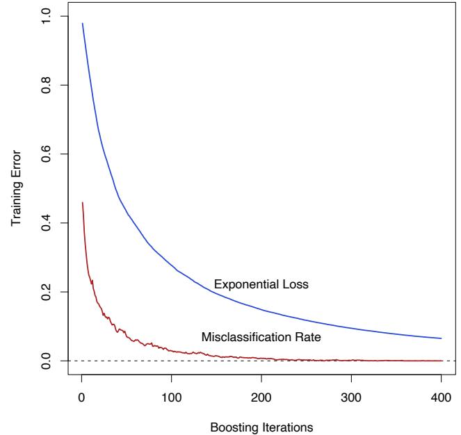
FIGURE 10.3. Simulated data, boosting with stumps: misclassification error rate on the training set, and average exponential loss: (1/N) P^{N i}=1 exp(−yif(xi)). After about 250 iterations, the misclassification error is zero, while the exponential loss continues to decrease.

10.5 Why Exponential Loss?

The AdaBoost.M1 algorithm was originally motivated from a very different perspective than presented in the previous section. Its equivalence to forward stagewise additive modeling based on exponential loss was only discovered five years after its inception. By studying the properties of the exponential loss criterion, one can gain insight into the procedure and discover ways it might be improved.

The principal attraction of exponential loss in the context of additive modeling is computational; it leads to the simple modular reweighting AdaBoost algorithm. However, it is of interest to inquire about its statistical properties. What does it estimate and how well is it being estimated? The first question is answered by seeking its population minimizer.

It is easy to show (Friedman et al., 2000) that

\[f^\*(x) = \arg\min\_{f(x)} \mathcal{E}\_{Y|x}(e^{-Yf(x)}) = \frac{1}{2} \log \frac{\Pr(Y = 1|x)}{\Pr(Y = -1|x)},\tag{10.16}\]

346 10. Boosting and Additive Trees

or equivalently

\[\Pr(Y=1|x) = \frac{1}{1+e^{-2f^\*(x)}}.\]

Thus, the additive expansion produced by AdaBoost is estimating onehalf the log-odds of P(Y = 1|x). This justifies using its sign as the classification rule in (10.1).

Another loss criterion with the same population minimizer is the binomial negative log-likelihood or deviance (also known as cross-entropy), interpreting f as the logit transform. Let

\[p(x) = \Pr(Y = 1 \mid x) = \frac{e^{f(x)}}{e^{-f(x)} + e^{f(x)}} = \frac{1}{1 + e^{-2f(x)}} \tag{10.17}\]

and define ^Y ′ = (^Y + 1)/^{2 ∈} {0, ¹}. Then the binomial log-likelihood loss function is

\[d(Y, p(x)) = Y' \log p(x) + (1 - Y') \log(1 - p(x)),\]

or equivalently the deviance is

\[-l(Y, f(x)) = \log\left(1 + e^{-2Yf(x)}\right). \tag{10.18}\]

Since the population maximizer of log-likelihood is at the true probabilities p(x) = Pr(Y = 1 | x), we see from (10.17) that the population minimizers of the deviance E^{Y |}x[−l(Y,f(x))] and E^{Y |}x[e⁻Y f(x) ] are the same. Thus, using either criterion leads to the same solution at the population level. Note that e⁻Y f itself is not a proper log-likelihood, since it is not the logarithm of any probability mass function for a binary random variable Y ∈ {−1, 1}.

10.6 Loss Functions and Robustness

In this section we examine the different loss functions for classification and regression more closely, and characterize them in terms of their robustness to extreme data.

Robust Loss Functions for Classification

Although both the exponential (10.8) and binomial deviance (10.18) yield the same solution when applied to the population joint distribution, the same is not true for finite data sets. Both criteria are monotone decreasing functions of the “margin” yf(x). In classification (with a −1/1 response) the margin plays a role analogous to the residuals y−f(x) in regression. The classification rule G(x) = sign[f(x)] implies that observations with positive margin yif(xi) > 0 are classified correctly whereas those with negative margin yif(xi) < 0 are misclassified. The decision boundary is defined by

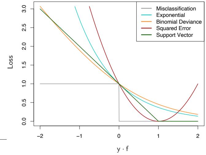
FIGURE 10.4. Loss functions for two-class classification. The response is y = ±1; the prediction is f, with class prediction sign(f). The losses are misclassification: I(sign(f) ̸= y); exponential: exp(−yf); binomial deviance: log(1 + exp(−2yf)); squared error: (y − f) ²; and support vector: (1 ⁻ yf)⁺ (see Section 12.3). Each function has been scaled so that it passes through the point (0, 1).

f(x) = 0. The goal of the classification algorithm is to produce positive margins as frequently as possible. Any loss criterion used for classification should penalize negative margins more heavily than positive ones since positive margin observations are already correctly classified.

Figure 10.4 shows both the exponential (10.8) and binomial deviance criteria as a function of the margin y · f(x). Also shown is misclassification loss L(y, f(x)) = I(y ·f(x) < 0), which gives unit penalty for negative margin values, and no penalty at all for positive ones. Both the exponential and deviance loss can be viewed as monotone continuous approximations to misclassification loss. They continuously penalize increasingly negative margin values more heavily than they reward increasingly positive ones. The difference between them is in degree. The penalty associated with binomial deviance increases linearly for large increasingly negative margin, whereas the exponential criterion increases the influence of such observations exponentially.

At any point in the training process the exponential criterion concentrates much more influence on observations with large negative margins. Binomial deviance concentrates relatively less influence on such observa-

348 10. Boosting and Additive Trees

tions, more evenly spreading the influence among all of the data. It is therefore far more robust in noisy settings where the Bayes error rate is not close to zero, and especially in situations where there is misspecification of the class labels in the training data. The performance of AdaBoost has been empirically observed to dramatically degrade in such situations.

Also shown in the figure is squared-error loss. The minimizer of the corresponding risk on the population is

\[f^\*(x) = \arg\min\_{f(x)} \mathcal{E}\_{Y|x} (Y - f(x))^2 = \mathcal{E}(Y \mid x) = 2 \cdot \Pr(Y = 1 \mid x) - 1. \tag{10.19}\]

As before the classification rule is G(x) = sign[f(x)]. Squared-error loss is not a good surrogate for misclassification error. As seen in Figure 10.4, it is not a monotone decreasing function of increasing margin yf(x). For margin values yif(xi) > 1 it increases quadratically, thereby placing increasing influence (error) on observations that are correctly classified with increasing certainty, thereby reducing the relative influence of those incorrectly classified yif(xi) < 0. Thus, if class assignment is the goal, a monotone decreasing criterion serves as a better surrogate loss function. Figure 12.4 on page 426 in Chapter 12 includes a modification of quadratic loss, the “Huberized” square hinge loss (Rosset et al., 2004b), which enjoys the favorable properties of the binomial deviance, quadratic loss and the SVM hinge loss. It has the same population minimizer as the quadratic (10.19), is zero for y ·f(x) > 1, and becomes linear for y ·f(x) < −1. Since quadratic functions are easier to compute with than exponentials, our experience suggests this to be a useful alternative to the binomial deviance.

With K-class classification, the response Y takes values in the unordered set G = {G1,…, Gk} (see Sections 2.4 and 4.4). We now seek a classifier G(x) taking values in G. It is sufficient to know the class conditional probabilities pk(x) = Pr(Y = Gk|x), k = 1, 2,…,K, for then the Bayes classifier is

\[G(x) = \mathcal{G}\_k \text{ where } k = \arg\max\_{\ell} p\_\ell(x). \tag{10.20}\]

In principal, though, we need not learn the pk(x), but simply which one is largest. However, in data mining applications the interest is often more in the class probabilities pℓ(x), ℓ = 1,…,K themselves, rather than in performing a class assignment. As in Section 4.4, the logistic model generalizes naturally to K classes,

\[p\_k(x) = \frac{e^{f\_k(x)}}{\sum\_{l=1}^K e^{f\_l(x)}},\tag{10.21}\]

which ensures that 0 ≤ pk(x) ≤ 1 and that they sum to one. Note that here we have K different functions, one per class. There is a redundancy in the functions fk(x), since adding an arbitrary h(x) to each leaves the model unchanged. Traditionally one of them is set to zero: for example, fK(x) = 0, as in (4.17). Here we prefer to retain the symmetry, and impose the constraint #^{K k}=1 fk(x) = 0. The binomial deviance extends naturally to the K-class multinomial deviance loss function:

\[\begin{aligned} L(y, p(x)) &= -\sum\_{k=1}^{K} I(y = \mathcal{G}\_k) \log p\_k(x) \\ &= -\sum\_{k=1}^{K} I(y = \mathcal{G}\_k) f\_k(x) + \log \left( \sum\_{\ell=1}^{K} e^{f\_\ell(x)} \right) . \end{aligned} \tag{10.22}\]

As in the two-class case, the criterion (10.22) penalizes incorrect predictions only linearly in their degree of incorrectness.

Zhu et al. (2005) generalize the exponential loss for K-class problems. See Exercise 10.5 for details.

Robust Loss Functions for Regression

In the regression setting, analogous to the relationship between exponential loss and binomial log-likelihood is the relationship between squared-error loss ^L(y, f(x)) = (y−f(x))² and absolute loss ^L(y, f(x)) = ^{| y}−f(x)|. The population solutions are f(x) = E(Y |x) for squared-error loss, and f(x) = median(Y |x) for absolute loss; for symmetric error distributions these are the same. However, on finite samples squared-error loss places much more emphasis on observations with large absolute residuals | yⁱ − f(xi)| during the fitting process. It is thus far less robust, and its performance severely degrades for long-tailed error distributions and especially for grossly mismeasured y-values (“outliers”). Other more robust criteria, such as absolute loss, perform much better in these situations. In the statistical robustness literature, a variety of regression loss criteria have been proposed that provide strong resistance (if not absolute immunity) to gross outliers while being nearly as efficient as least squares for Gaussian errors. They are often better than either for error distributions with moderately heavy tails. One such criterion is the Huber loss criterion used for M-regression (Huber, 1964)

\[L(y, f(x)) = \begin{cases} \begin{array}{c} [y - f(x)]^2 \\ 2\delta |y - f(x)| - \delta^2 \end{array} & \text{otherwise.} \end{cases} \tag{10.23}\]

Figure 10.5 compares these three loss functions.

These considerations suggest than when robustness is a concern, as is especially the case in data mining applications (see Section 10.7), squarederror loss for regression and exponential loss for classification are not the best criteria from a statistical perspective. However, they both lead to the elegant modular boosting algorithms in the context of forward stagewise additive modeling. For squared-error loss one simply fits the base learner to the residuals from the current model yⁱ − fm−1(xi) at each step. For

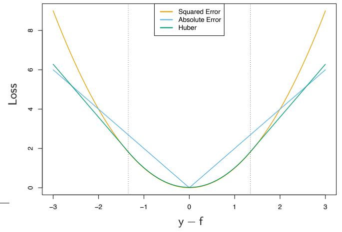
FIGURE 10.5. A comparison of three loss functions for regression, plotted as a function of the margin y−f. The Huber loss function combines the good properties of squared-error loss near zero and absolute error loss when |y − f| is large.

exponential loss one performs a weighted fit of the base learner to the output values yi, with weights wⁱ = exp(−yifm−1(xi)). Using other more robust criteria directly in their place does not give rise to such simple feasible boosting algorithms. However, in Section 10.10.2 we show how one can derive simple elegant boosting algorithms based on any differentiable loss criterion, thereby producing highly robust boosting procedures for data mining.

10.7 “Off-the-Shelf” Procedures for Data Mining

Predictive learning is an important aspect of data mining. As can be seen from this book, a wide variety of methods have been developed for predictive learning from data. For each particular method there are situations for which it is particularly well suited, and others where it performs badly compared to the best that can be done with that data. We have attempted to characterize appropriate situations in our discussions of each of the respective methods. However, it is seldom known in advance which procedure will perform best or even well for any given problem. Table 10.1 summarizes some of the characteristics of a number of learning methods.

Industrial and commercial data mining applications tend to be especially challenging in terms of the requirements placed on learning procedures. Data sets are often very large in terms of number of observations and number of variables measured on each of them. Thus, computational con-

Characteristic	Neural	SVM	Trees	MARS	k-NN,
	Nets				Kernels
Natural handling of data of “mixed” type	▼	▼	▲	▲	▼
Handling of missing values	▼	▼	▲	▲	▲
Robustness to outliers in input space	▼	▼	▲	▼	▲
Insensitive to monotone transformations of inputs	▼	▼	▲	▼	▼
Computational scalability (large N)	▼	▼	▲	▲	▼
Ability to deal with irrel evant inputs	▼	▼	▲	▲	▼
Ability to extract linear combinations of features	▲	▲	▼	▼	◆
Interpretability	▼	▼	◆	▲	▼
Predictive power	▲	▲	▼	◆	▲

TABLE 10.1. Some characteristics of different learning methods. Key: ▲= good, ◆=fair, and ▼=poor.

siderations play an important role. Also, the data are usually messy: the inputs tend to be mixtures of quantitative, binary, and categorical variables, the latter often with many levels. There are generally many missing values, complete observations being rare. Distributions of numeric predictor and response variables are often long-tailed and highly skewed. This is the case for the spam data (Section 9.1.2); when fitting a generalized additive model, we first log-transformed each of the predictors in order to get a reasonable fit. In addition they usually contain a substantial fraction of gross mis-measurements (outliers). The predictor variables are generally measured on very different scales.

In data mining applications, usually only a small fraction of the large number of predictor variables that have been included in the analysis are actually relevant to prediction. Also, unlike many applications such as pattern recognition, there is seldom reliable domain knowledge to help create especially relevant features and/or filter out the irrelevant ones, the inclusion of which dramatically degrades the performance of many methods.

In addition, data mining applications generally require interpretable models. It is not enough to simply produce predictions. It is also desirable to have information providing qualitative understanding of the relationship

352 10. Boosting and Additive Trees

between joint values of the input variables and the resulting predicted response value. Thus, black box methods such as neural networks, which can be quite useful in purely predictive settings such as pattern recognition, are far less useful for data mining.

These requirements of speed, interpretability and the messy nature of the data sharply limit the usefulness of most learning procedures as offthe-shelf methods for data mining. An “off-the-shelf” method is one that can be directly applied to the data without requiring a great deal of timeconsuming data preprocessing or careful tuning of the learning procedure.

Of all the well-known learning methods, decision trees come closest to meeting the requirements for serving as an off-the-shelf procedure for data mining. They are relatively fast to construct and they produce interpretable models (if the trees are small). As discussed in Section 9.2, they naturally incorporate mixtures of numeric and categorical predictor variables and missing values. They are invariant under (strictly monotone) transformations of the individual predictors. As a result, scaling and/or more general transformations are not an issue, and they are immune to the effects of predictor outliers. They perform internal feature selection as an integral part of the procedure. They are thereby resistant, if not completely immune, to the inclusion of many irrelevant predictor variables. These properties of decision trees are largely the reason that they have emerged as the most popular learning method for data mining.

Trees have one aspect that prevents them from being the ideal tool for predictive learning, namely inaccuracy. They seldom provide predictive accuracy comparable to the best that can be achieved with the data at hand. As seen in Section 10.1, boosting decision trees improves their accuracy, often dramatically. At the same time it maintains most of their desirable properties for data mining. Some advantages of trees that are sacrificed by boosting are speed, interpretability, and, for AdaBoost, robustness against overlapping class distributions and especially mislabeling of the training data. A gradient boosted model (GBM) is a generalization of tree boosting that attempts to mitigate these problems, so as to produce an accurate and effective off-the-shelf procedure for data mining.

10.8 Example: Spam Data

Before we go into the details of gradient boosting, we demonstrate its abilities on a two-class classification problem. The spam data are introduced in Chapter 1, and used as an example for many of the procedures in Chapter 9 (Sections 9.1.2, 9.2.5, 9.3.1 and 9.4.1).

Applying gradient boosting to these data resulted in a test error rate of 4.5%, using the same test set as was used in Section 9.1.2. By comparison, an additive logistic regression achieved 5.5%, a CART tree fully grown and pruned by cross-validation 8.7%, and MARS 5.5%. The standard error of these estimates is around 0.6%, although gradient boosting is significantly better than all of them using the McNemar test (Exercise 10.6).

In Section 10.13 below we develop a relative importance measure for each predictor, as well as a partial dependence plot describing a predictor’s contribution to the fitted model. We now illustrate these for the spam data.

Figure 10.6 displays the relative importance spectrum for all 57 predictor variables. Clearly some predictors are more important than others in separating spam from email. The frequencies of the character strings !, $, hp, and remove are estimated to be the four most relevant predictor variables. At the other end of the spectrum, the character strings 857, 415, table, and 3d have virtually no relevance.

The quantity being modeled here is the log-odds of spam versus email

\[f(x) = \log \frac{\Pr(\mathsf{spam}|x)}{\Pr(\mathsf{email}|x)} \tag{10.24}\]

(see Section 10.13 below). Figure 10.7 shows the partial dependence of the log-odds on selected important predictors, two positively associated with spam (! and remove), and two negatively associated (edu and hp). These particular dependencies are seen to be essentially monotonic. There is a general agreement with the corresponding functions found by the additive logistic regression model; see Figure 9.1 on page 303.

Running a gradient boosted model on these data with J = 2 terminalnode trees produces a purely additive (main effects) model for the logodds, with a corresponding error rate of 4.7%, as compared to 4.5% for the full gradient boosted model (with J = 5 terminal-node trees). Although not significant, this slightly higher error rate suggests that there may be interactions among some of the important predictor variables. This can be diagnosed through two-variable partial dependence plots. Figure 10.8 shows one of the several such plots displaying strong interaction effects.

One sees that for very low frequencies of hp, the log-odds of spam are greatly increased. For high frequencies of hp, the log-odds of spam tend to be much lower and roughly constant as a function of !. As the frequency of hp decreases, the functional relationship with ! strengthens.

10.9 Boosting Trees

Regression and classification trees are discussed in detail in Section 9.2. They partition the space of all joint predictor variable values into disjoint regions R^j , j = 1, 2,…,J, as represented by the terminal nodes of the tree. A constant γ^j is assigned to each such region and the predictive rule is

\[x \in R\_j \Rightarrow f(x) = \gamma\_j.\]

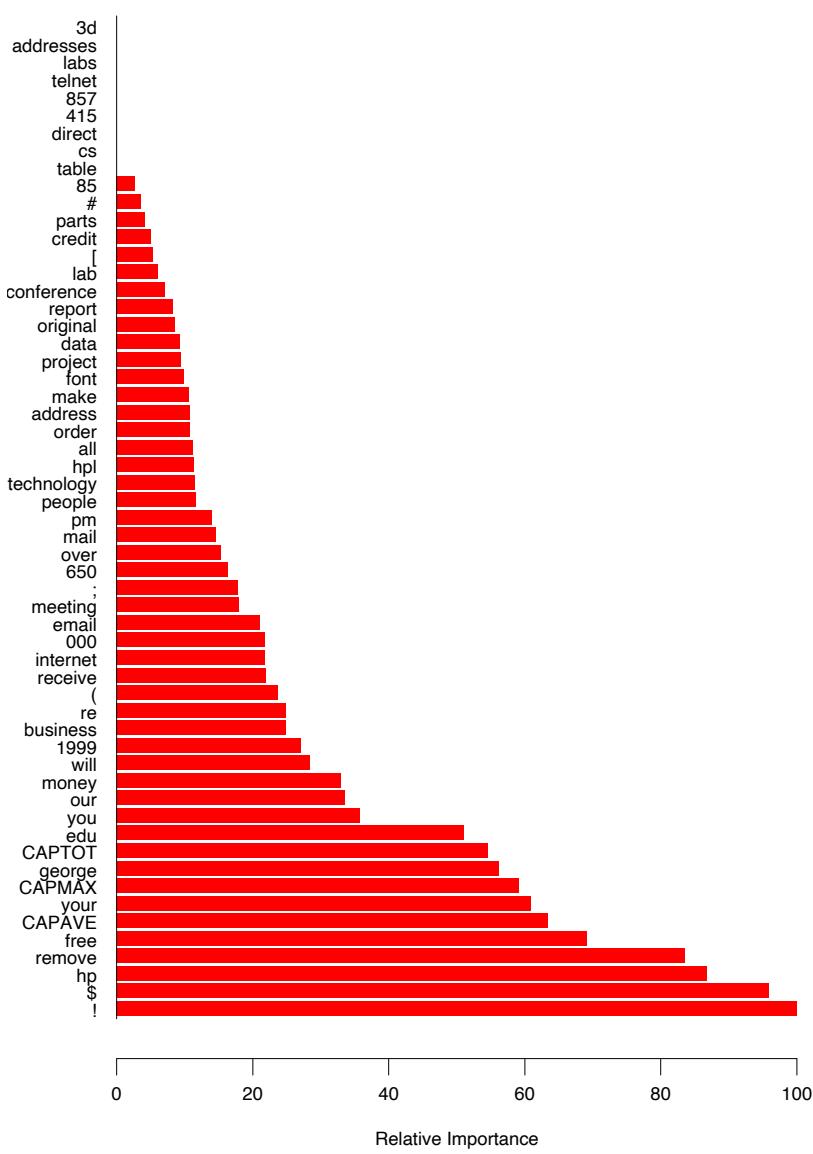
FIGURE 10.6. Predictor variable importance spectrum for the spam data. The variable names are written on the vertical axis.

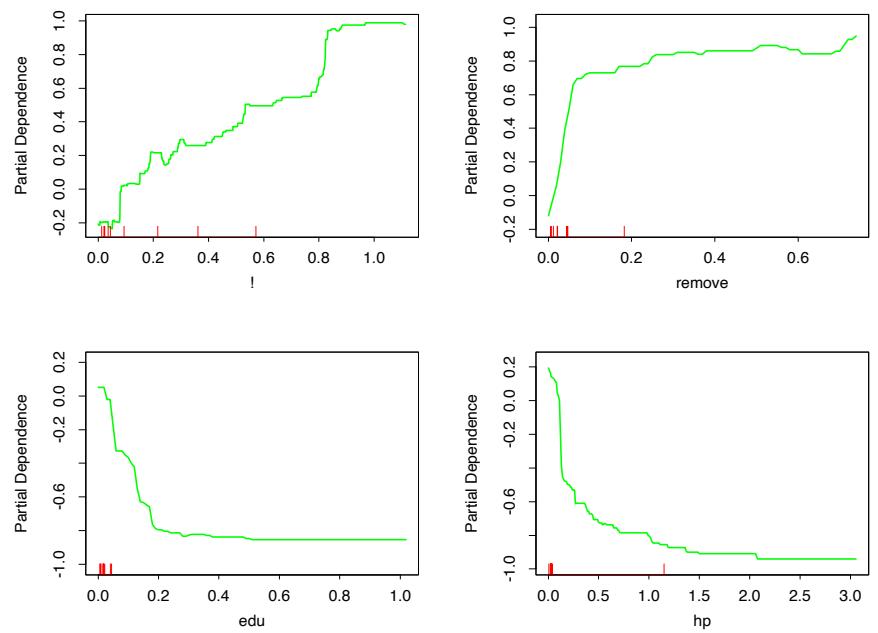
FIGURE 10.7. Partial dependence of log-odds of spam on four important predictors. The red ticks at the base of the plots are deciles of the input variable.

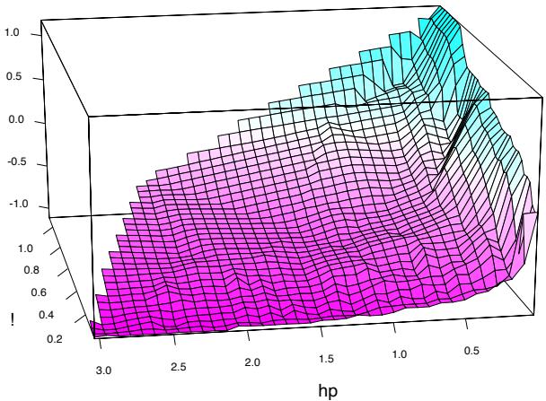
FIGURE 10.8. Partial dependence of the log-odds of spam vs. email as a function of joint frequencies of hp and the character !.

356 10. Boosting and Additive Trees

Thus a tree can be formally expressed as

\[T(x; \Theta) = \sum\_{j=1}^{J} \gamma\_j I(x \in R\_j),\tag{10.25}\]

with parameters ^{Θ =} {R^j , ^γj}^{J 1} . J is usually treated as a meta-parameter. The parameters are found by minimizing the empirical risk

\[\hat{\Theta} = \arg\min\_{\Theta} \sum\_{j=1}^{J} \sum\_{x\_i \in R\_j} L(y\_i, \gamma\_j). \tag{10.26}\]

This is a formidable combinatorial optimization problem, and we usually settle for approximate suboptimal solutions. It is useful to divide the optimization problem into two parts:

• Finding γ^j given R^j : Given the R^j , estimating the γ^j is typically trivial, and often ˆγ^j = ¯y^j , the mean of the yⁱ falling in region R^j . For misclassification loss, ˆγ^j is the modal class of the observations falling in region R^j .
• Finding R^j : This is the difficult part, for which approximate solutions are found. Note also that finding the R^j entails estimating the γ^j as well. A typical strategy is to use a greedy, top-down recursive partitioning algorithm to find the R^j . In addition, it is sometimes necessary to approximate (10.26) by a smoother and more convenient criterion for optimizing the R^j :

\[\tilde{\Theta} = \arg\min\_{\Theta} \sum\_{i=1}^{N} \tilde{L}(y\_i, T(x\_i, \Theta)). \tag{10.27}\]

Then given the Rˆ^j = R˜^j , the γ^j can be estimated more precisely using the original criterion.

In Section 9.2 we described such a strategy for classification trees. The Gini index replaced misclassification loss in the growing of the tree (identifying the R^j ).

The boosted tree model is a sum of such trees,

\[f\_M(x) = \sum\_{m=1}^M T(x; \Theta\_m),\tag{10.28}\]

induced in a forward stagewise manner (Algorithm 10.2). At each step in the forward stagewise procedure one must solve

\[\hat{\Theta}\_m = \arg\min\_{\Theta\_m} \sum\_{i=1}^N L\left(y\_i, f\_{m-1}(x\_i) + T(x\_i; \Theta\_m)\right) \tag{10.29}\]

for the region set and constants ^{Θm =} {Rjm, ^γjm}J^{m 1} of the next tree, given the current model fm−1(x).

Given the regions Rjm, finding the optimal constants γjm in each region is typically straightforward:

\[\hat{\gamma}\_{jm} = \arg\min\_{\gamma\_{jm}} \sum\_{x\_i \in R\_{jm}} L\left(y\_i, f\_{m-1}(x\_i) + \gamma\_{jm}\right). \tag{10.30}\]

Finding the regions is difficult, and even more difficult than for a single tree. For a few special cases, the problem simplifies.

For squared-error loss, the solution to (10.29) is no harder than for a single tree. It is simply the regression tree that best predicts the current residuals yⁱ − fm−1(xi), and ˆγjm is the mean of these residuals in each corresponding region.

For two-class classification and exponential loss, this stagewise approach gives rise to the AdaBoost method for boosting classification trees (Algorithm 10.1). In particular, if the trees T(x; Θm) are restricted to be scaled classification trees, then we showed in Section 10.4 that the solution to (10.29) is the tree that minimizes the weighted error rate #^{N i}=1 ^w(m) ⁱ I(yⁱ ̸= T(xi; Θm)) with weights w(m) ⁱ = e⁻yifm−1(xi) . By a scaled classification tree, we mean βmT(x; Θm), with the restriction that γjm ∈ {−1, 1}).

Without this restriction, (10.29) still simplifies for exponential loss to a weighted exponential criterion for the new tree:

\[\hat{\Theta}\_m = \arg\min\_{\Theta\_m} \sum\_{i=1}^N w\_i^{(m)} \exp[-y\_i T(x\_i; \Theta\_m)].\tag{10.31}\]

It is straightforward to implement a greedy recursive-partitioning algorithm using this weighted exponential loss as a splitting criterion. Given the Rjm, one can show (Exercise 10.7) that the solution to (10.30) is the weighted log-odds in each corresponding region

\[\hat{\gamma}\_{jm} = \log \frac{\sum\_{x\_i \in R\_{jm}} w\_i^{(m)} I(y\_i = 1)}{\sum\_{x\_i \in R\_{jm}} w\_i^{(m)} I(y\_i = -1)}. \tag{10.32}\]

This requires a specialized tree-growing algorithm; in practice, we prefer the approximation presented below that uses a weighted least squares regression tree.

Using loss criteria such as the absolute error or the Huber loss (10.23) in place of squared-error loss for regression, and the deviance (10.22) in place of exponential loss for classification, will serve to robustify boosting trees. Unfortunately, unlike their nonrobust counterparts, these robust criteria do not give rise to simple fast boosting algorithms.

For more general loss criteria the solution to (10.30), given the Rjm, is typically straightforward since it is a simple “location” estimate. For

358 10. Boosting and Additive Trees

absolute loss it is just the median of the residuals in each respective region. For the other criteria fast iterative algorithms exist for solving (10.30), and usually their faster “single-step” approximations are adequate. The problem is tree induction. Simple fast algorithms do not exist for solving (10.29) for these more general loss criteria, and approximations like (10.27) become essential.

10.10 Numerical Optimization via Gradient Boosting

Fast approximate algorithms for solving (10.29) with any differentiable loss criterion can be derived by analogy to numerical optimization. The loss in using f(x) to predict y on the training data is

\[L(f) = \sum\_{i=1}^{N} L(y\_i, f(x\_i)).\tag{10.33}\]

The goal is to minimize L(f) with respect to f, where here f(x) is constrained to be a sum of trees (10.28). Ignoring this constraint, minimizing (10.33) can be viewed as a numerical optimization

\[ \hat{\mathbf{f}} = \arg\min\_{\mathbf{f}} L(\mathbf{f}), \tag{10.34} \]

where the “parameters” ^{f ∈} IR^N are the values of the approximating function f(xi) at each of the N data points xi:

\[\mathbf{f} = \{f(x\_1), f(x\_2)), \dots, f(x\_N)\}.\]

Numerical optimization procedures solve (10.34) as a sum of component vectors

\[\mathbf{f}\_M = \sum\_{m=0}^M \mathbf{h}\_m \,, \quad \mathbf{h}\_m \in \mathbb{R}^N,\]

where f⁰ = h⁰ is an initial guess, and each successive f^m is induced based on the current parameter vector fm−1, which is the sum of the previously induced updates. Numerical optimization methods differ in their prescriptions for computing each increment vector h^m (“step”).

10.10.1 Steepest Descent

Steepest descent chooses ^{hm = −}ρmg^m where ^ρm is a scalar and ^{gm ∈} IR^N is the gradient of L(f) evaluated at f = fm−1. The components of the gradient g^m are

\[g\_{im} = \left[\frac{\partial L(y\_i, f(x\_i))}{\partial f(x\_i)}\right]\_{f(x\_i) = f\_{m-1}(x\_i)}\tag{10.35}\]

The step length ρ^m is the solution to

\[\rho\_m = \arg\min\_{\rho} L(\mathbf{f}\_{m-1} - \rho \mathbf{g}\_m). \tag{10.36}\]

The current solution is then updated

\[\mathbf{f}\_m = \mathbf{f}\_{m-1} - \rho\_m \mathbf{g}\_m\]

and the process repeated at the next iteration. Steepest descent can be viewed as a very greedy strategy, since ⁻g^m is the local direction in IR^N for which L(f) is most rapidly decreasing at f = fm−1.

10.10.2 Gradient Boosting

Forward stagewise boosting (Algorithm 10.2) is also a very greedy strategy. At each step the solution tree is the one that maximally reduces (10.29), given the current model fm−¹ and its fits fm−1(xi). Thus, the tree predictions T(xi; Θm) are analogous to the components of the negative gradient (10.35). The principal difference between them is that the tree components t^m = (T(x1; Θm),…,T(x^N ; Θm) are not independent. They are constrained to be the predictions of a Jm-terminal node decision tree, whereas the negative gradient is the unconstrained maximal descent direction.

The solution to (10.30) in the stagewise approach is analogous to the line search (10.36) in steepest descent. The difference is that (10.30) performs a separate line search for those components of t^m that correspond to each separate terminal region {T(xi; Θm)}^xi∈Rjm.

If minimizing loss on the training data (10.33) were the only goal, steepest descent would be the preferred strategy. The gradient (10.35) is trivial to calculate for any differentiable loss function L(y, f(x)), whereas solving (10.29) is difficult for the robust criteria discussed in Section 10.6. Unfortunately the gradient (10.35) is defined only at the training data points xi, whereas the ultimate goal is to generalize fM(x) to new data not represented in the training set.

A possible resolution to this dilemma is to induce a tree T(x; Θm) at the mth iteration whose predictions t^m are as close as possible to the negative gradient. Using squared error to measure closeness, this leads us to

\[\tilde{\Theta}\_m = \arg\min\_{\Theta} \sum\_{i=1}^N \left( -g\_{im} - T(x\_i; \Theta) \right)^2. \tag{10.37}\]

That is, one fits the tree T to the negative gradient values (10.35) by least squares. As noted in Section 10.9 fast algorithms exist for least squares decision tree induction. Although the solution regions R˜jm to (10.37) will not be identical to the regions Rjm that solve (10.29), it is generally similar enough to serve the same purpose. In any case, the forward stagewise

Setting	Loss Function	−∂L(yi, f(xi))/∂f(xi)
Regression	1 − f(xi)]2 2 [yi	yi − f(xi)
Regression	yi − f(xi)	sign[yi − f(xi)]
Regression	Huber	yi − f(xi) for yi − f(xi) ≤ δm δmsign[yi − f(xi)] for yi − f(xi) > δm where δm = αth-quantile{ yi − f(xi) }
Classification	Deviance	kth component: I(yi = Gk) − pk(xi)

TABLE 10.2. Gradients for commonly used loss functions.

boosting procedure, and top-down decision tree induction, are themselves approximation procedures. After constructing the tree (10.37), the corresponding constants in each region are given by (10.30).

Table 10.2 summarizes the gradients for commonly used loss functions. For squared error loss, the negative gradient is just the ordinary residual −gim = yⁱ − fm−1(xi), so that (10.37) on its own is equivalent standard least squares boosting. With absolute error loss, the negative gradient is the sign of the residual, so at each iteration (10.37) fits the tree to the sign of the current residuals by least squares. For Huber M-regression, the negative gradient is a compromise between these two (see the table).

For classification the loss function is the multinomial deviance (10.22), and K least squares trees are constructed at each iteration. Each tree Tkm is fit to its respective negative gradient vector gkm,

\[\begin{aligned} -g\_{ikm} &= \frac{\partial L\left(y\_i, f\_{1m}(x\_i), \dots, f\_{1m}(x\_i)\right)}{\partial f\_{km}(x\_i)}\\ &= \quad I(y\_i = \mathcal{G}\_k) - p\_k(x\_i), \end{aligned} \tag{10.38}\]

with pk(x) given by (10.21). Although K separate trees are built at each iteration, they are related through (10.21). For binary classification (K = 2), only one tree is needed (exercise 10.10).

10.10.3 Implementations of Gradient Boosting

Algorithm 10.3 presents the generic gradient tree-boosting algorithm for regression. Specific algorithms are obtained by inserting different loss criteria L(y, f(x)). The first line of the algorithm initializes to the optimal constant model, which is just a single terminal node tree. The components of the negative gradient computed at line 2(a) are referred to as generalized or pseudo residuals, r. Gradients for commonly used loss functions are summarized in Table 10.2.

.

Algorithm 10.3 Gradient Tree Boosting Algorithm.

• 1. Initialize f0(x) = arg min^γ #^{N i}=1 L(yi, γ).
• 2. For m = 1 to M:
  • 1. For i = 1, 2,…,N compute

\[r\_{im} = -\left[\frac{\partial L(y\_i, f(x\_i))}{\partial f(x\_i)}\right]\_{f = f\_{m-1}}\]

• 2. Fit a regression tree to the targets rim giving terminal regions Rjm, j = 1, 2,…,Jm.
• 3. For j = 1, 2,…,J^m compute

\[\gamma\_{jm} = \arg\min\_{\gamma} \sum\_{x\_i \in R\_{jm}} L\left(y\_i, f\_{m-1}(x\_i) + \gamma\right).\]

• 4. Update fm(x) = fm−1(x) + #^{Jm j}=1 γjmI(x ∈ Rjm).
• 3. Output ˆf(x) = fM(x).

The algorithm for classification is similar. Lines 2(a)–(d) are repeated K times at each iteration m, once for each class using (10.38). The result at line 3 is K different (coupled) tree expansions fkM(x), k = 1, 2,…,K. These produce probabilities via (10.21) or do classification as in (10.20). Details are given in Exercise 10.9. Two basic tuning parameters are the number of iterations M and the sizes of each of the constituent trees Jm, m = 1, 2,…,M.

The original implementation of this algorithm was called MART for “multiple additive regression trees,” and was referred to in the first edition of this book. Many of the figures in this chapter were produced by MART. Gradient boosting as described here is implemented in the R gbm package (Ridgeway, 1999, “Gradient Boosted Models”), and is freely available. The gbm package is used in Section 10.14.2, and extensively in Chapters 16 and 15. Another R implementation of boosting is mboost (Hothorn and B¨uhlmann, 2006). A commercial implementation of gradient boosting/MART called TreeNet is available from Salford Systems, Inc.

10.11 Right-Sized Trees for Boosting

Historically, boosting was considered to be a technique for combining models, here trees. As such, the tree building algorithm was regarded as a

362 10. Boosting and Additive Trees

primitive that produced models to be combined by the boosting procedure. In this scenario, the optimal size of each tree is estimated separately in the usual manner when it is built (Section 9.2). A very large (oversized) tree is first induced, and then a bottom-up procedure is employed to prune it to the estimated optimal number of terminal nodes. This approach assumes implicitly that each tree is the last one in the expansion (10.28). Except perhaps for the very last tree, this is clearly a very poor assumption. The result is that trees tend to be much too large, especially during the early iterations. This substantially degrades performance and increases computation.

The simplest strategy for avoiding this problem is to restrict all trees to be the same size, J^m = J ∀m. At each iteration a J-terminal node regression tree is induced. Thus J becomes a meta-parameter of the entire boosting procedure, to be adjusted to maximize estimated performance for the data at hand.

One can get an idea of useful values for J by considering the properties of the “target” function

\[\eta = \arg\min\_{f} \mathcal{E}\_{XY} L(Y, f(X)). \tag{10.39}\]

Here the expected value is over the population joint distribution of (X, Y ). The target function η(x) is the one with minimum prediction risk on future data. This is the function we are trying to approximate.

One relevant property of η(X) is the degree to which the coordinate variables X^T = (X1, X2,…,Xp) interact with one another. This is captured by its ANOVA (analysis of variance) expansion

\[\eta(X) = \sum\_{j} \eta\_{j}(X\_{j}) + \sum\_{jk} \eta\_{jk}(X\_{j}, X\_{k}) + \sum\_{jkl} \eta\_{jkl}(X\_{j}, X\_{k}, X\_{l}) + \cdots \text{ (10.40)}\]

The first sum in (10.40) is over functions of only a single predictor variable X^j . The particular functions η^j (X^j ) are those that jointly best approximate η(X) under the loss criterion being used. Each such η^j (X^j ) is called the “main effect” of X^j . The second sum is over those two-variable functions that when added to the main effects best fit η(X). These are called the second-order interactions of each respective variable pair (X^j , Xk). The third sum represents third-order interactions, and so on. For many problems encountered in practice, low-order interaction effects tend to dominate. When this is the case, models that produce strong higher-order interaction effects, such as large decision trees, suffer in accuracy.

The interaction level of tree-based approximations is limited by the tree size J. Namely, no interaction effects of level greater that J − 1 are possible. Since boosted models are additive in the trees (10.28), this limit extends to them as well. Setting J = 2 (single split “decision stump”) produces boosted models with only main effects; no interactions are permitted. With J = 3, two-variable interaction effects are also allowed, and

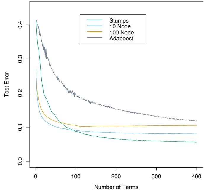
FIGURE 10.9. Boosting with different sized trees, applied to the example (10.2) used in Figure 10.2. Since the generative model is additive, stumps perform the best. The boosting algorithm used the binomial deviance loss in Algorithm 10.3; shown for comparison is the AdaBoost Algorithm 10.1.

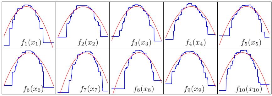
so on. This suggests that the value chosen for J should reflect the level of dominant interactions of η(x). This is of course generally unknown, but in most situations it will tend to be low. Figure 10.9 illustrates the effect of interaction order (choice of J) on the simulation example (10.2). The generative function is additive (sum of quadratic monomials), so boosting models with J > 2 incurs unnecessary variance and hence the higher test error. Figure 10.10 compares the coordinate functions found by boosted stumps with the true functions.

Although in many applications J = 2 will be insufficient, it is unlikely that J > 10 will be required. Experience so far indicates that 4 ≤ J ≤ 8 works well in the context of boosting, with results being fairly insensitive to particular choices in this range. One can fine-tune the value for J by trying several different values and choosing the one that produces the lowest risk on a validation sample. However, this seldom provides significant improvement over using J ≃ 6.

Coordinate Functions for Additive Logistic Trees

FIGURE 10.10. Coordinate functions estimated by boosting stumps for the simulated example used in Figure 10.9. The true quadratic functions are shown for comparison.

10.12 Regularization

Besides the size of the constituent trees, J, the other meta-parameter of gradient boosting is the number of boosting iterations M. Each iteration usually reduces the training risk L(fM), so that for M large enough this risk can be made arbitrarily small. However, fitting the training data too well can lead to overfitting, which degrades the risk on future predictions. Thus, there is an optimal number M^∗ minimizing future risk that is application dependent. A convenient way to estimate M^∗ is to monitor prediction risk as a function of M on a validation sample. The value of M that minimizes this risk is taken to be an estimate of M^∗. This is analogous to the early stopping strategy often used with neural networks (Section 11.4).

10.12.1 Shrinkage

Controlling the value of M is not the only possible regularization strategy. As with ridge regression and neural networks, shrinkage techniques can be employed as well (see Sections 3.4.1 and 11.5). The simplest implementation of shrinkage in the context of boosting is to scale the contribution of each tree by a factor 0 < ν < 1 when it is added to the current approximation. That is, line 2(d) of Algorithm 10.3 is replaced by

\[f\_m(x) = f\_{m-1}(x) + \nu \cdot \sum\_{j=1}^{J} \gamma\_{jm} I(x \in R\_{jm}).\tag{10.41}\]

The parameter ν can be regarded as controlling the learning rate of the boosting procedure. Smaller values of ν (more shrinkage) result in larger training risk for the same number of iterations M. Thus, both ν and M control prediction risk on the training data. However, these parameters do not operate independently. Smaller values of ν lead to larger values of M for the same training risk, so that there is a tradeoff between them.

Empirically it has been found (Friedman, 2001) that smaller values of ν favor better test error, and require correspondingly larger values of M. In fact, the best strategy appears to be to set ν to be very small (ν < 0.1) and then choose M by early stopping. This yields dramatic improvements (over no shrinkage ν = 1) for regression and for probability estimation. The corresponding improvements in misclassification risk via (10.20) are less, but still substantial. The price paid for these improvements is computational: smaller values of ν give rise to larger values of M, and computation is proportional to the latter. However, as seen below, many iterations are generally computationally feasible even on very large data sets. This is partly due to the fact that small trees are induced at each step with no pruning.

Figure 10.11 shows test error curves for the simulated example (10.2) of Figure 10.2. A gradient boosted model (MART) was trained using binomial deviance, using either stumps or six terminal-node trees, and with or without shrinkage. The benefits of shrinkage are evident, especially when the binomial deviance is tracked. With shrinkage, each test error curve reaches a lower value, and stays there for many iterations.

Section 16.2.1 draws a connection between forward stagewise shrinkage in boosting and the use of an L¹ penalty for regularizing model parameters (the “lasso”). We argue that L¹ penalties may be superior to the L² penalties used by methods such as the support vector machine.

10.12.2 Subsampling

We saw in Section 8.7 that bootstrap averaging (bagging) improves the performance of a noisy classifier through averaging. Chapter 15 discusses in some detail the variance-reduction mechanism of this sampling followed by averaging. We can exploit the same device in gradient boosting, both to improve performance and computational efficiency.

With stochastic gradient boosting (Friedman, 1999), at each iteration we sample a fraction η of the training observations (without replacement), and grow the next tree using that subsample. The rest of the algorithm is identical. A typical value for η can be ^{1 2} , although for large N, η can be substantially smaller than ¹ 2 .

Not only does the sampling reduce the computing time by the same fraction η, but in many cases it actually produces a more accurate model.

Figure 10.12 illustrates the effect of subsampling using the simulated example (10.2), both as a classification and as a regression example. We see in both cases that sampling along with shrinkage slightly outperformed the rest. It appears here that subsampling without shrinkage does poorly.

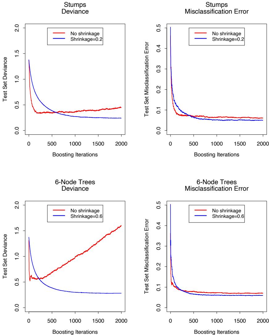
FIGURE 10.11. Test error curves for simulated example (10.2) of Figure 10.9, using gradient boosting (MART). The models were trained using binomial deviance, either stumps or six terminal-node trees, and with or without shrinkage. The left panels report test deviance, while the right panels show misclassification error. The beneficial effect of shrinkage can be seen in all cases, especially for deviance in the left panels.

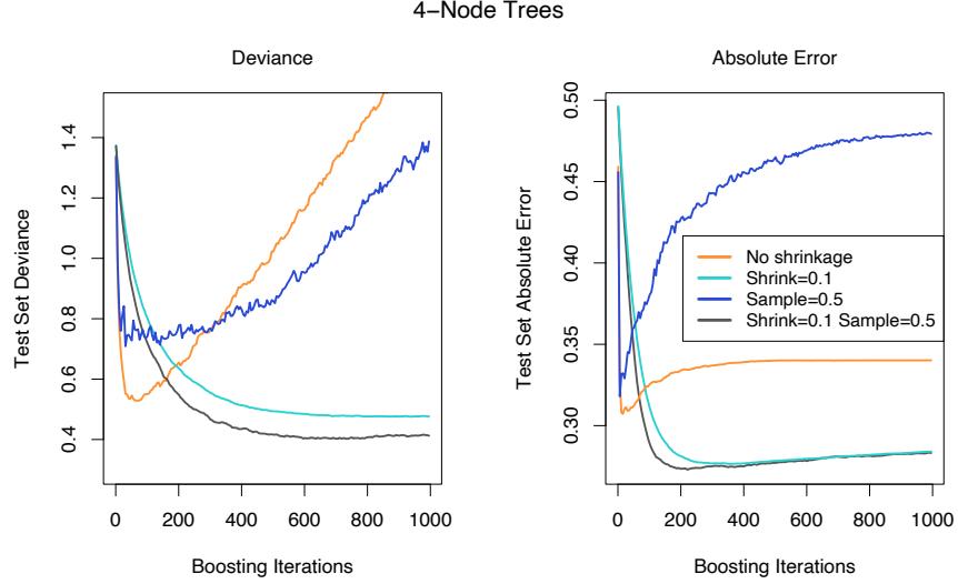
FIGURE 10.12. Test-error curves for the simulated example (10.2), showing the effect of stochasticity. For the curves labeled “Sample= 0.5”, a different 50% subsample of the training data was used each time a tree was grown. In the left panel the models were fit by gbm using a binomial deviance loss function; in the right-hand panel using square-error loss.

The downside is that we now have four parameters to set: J, M, ν and η. Typically some early explorations determine suitable values for J, ν and η, leaving M as the primary parameter.

10.13 Interpretation

Single decision trees are highly interpretable. The entire model can be completely represented by a simple two-dimensional graphic (binary tree) that is easily visualized. Linear combinations of trees (10.28) lose this important feature, and must therefore be interpreted in a different way.

10.13.1 Relative Importance of Predictor Variables

In data mining applications the input predictor variables are seldom equally relevant. Often only a few of them have substantial influence on the response; the vast majority are irrelevant and could just as well have not been included. It is often useful to learn the relative importance or contribution of each input variable in predicting the response.

368 10. Boosting and Additive Trees

For a single decision tree T, Breiman et al. (1984) proposed

\[\mathcal{T}\_{\ell}^{2}(T) = \sum\_{t=1}^{J-1} i\_{t}^{2} \, I(v(t) = \ell) \tag{10.42}\]

as a measure of relevance for each predictor variable Xℓ. The sum is over the J − 1 internal nodes of the tree. At each such node t, one of the input variables Xv(t) is used to partition the region associated with that node into two subregions; within each a separate constant is fit to the response values. The particular variable chosen is the one that gives maximal estimated improvement ˆı 2 ^t in squared error risk over that for a constant fit over the entire region. The squared relative importance of variable X^ℓ is the sum of such squared improvements over all internal nodes for which it was chosen as the splitting variable.

This importance measure is easily generalized to additive tree expansions (10.28); it is simply averaged over the trees

\[\mathcal{T}\_{\ell}^{2} = \frac{1}{M} \sum\_{m=1}^{M} \mathcal{T}\_{\ell}^{2}(T\_{m}). \tag{10.43}\]

Due to the stabilizing effect of averaging, this measure turns out to be more reliable than is its counterpart (10.42) for a single tree. Also, because of shrinkage (Section 10.12.1) the masking of important variables by others with which they are highly correlated is much less of a problem. Note that (10.42) and (10.43) refer to squared relevance; the actual relevances are their respective square roots. Since these measures are relative, it is customary to assign the largest a value of 100 and then scale the others accordingly. Figure 10.6 shows the relevant importance of the 57 inputs in predicting spam versus email.

For K-class classification, K separate models fk(x), k = 1, 2,…,K are induced, each consisting of a sum of trees

\[f\_k(x) = \sum\_{m=1}^{M} T\_{km}(x). \tag{10.44}\]

In this case (10.43) generalizes to

\[\mathcal{T}\_{\ell k}^{2} = \frac{1}{M} \sum\_{m=1}^{M} \mathcal{T}\_{\ell}^{2}(T\_{km}). \tag{10.45}\]

Here Iℓ^k is the relevance of X^ℓ in separating the class k observations from the other classes. The overall relevance of X^ℓ is obtained by averaging over all of the classes

\[\mathcal{T}\_{\ell}^{2} = \frac{1}{K} \sum\_{k=1}^{K} \mathcal{T}\_{\ell k}^{2}. \tag{10.46}\]

Figures 10.23 and 10.24 illustrate the use of these averaged and separate relative importances.

10.13.2 Partial Dependence Plots

After the most relevant variables have been identified, the next step is to attempt to understand the nature of the dependence of the approximation f(X) on their joint values. Graphical renderings of the f(X) as a function of its arguments provides a comprehensive summary of its dependence on the joint values of the input variables.

Unfortunately, such visualization is limited to low-dimensional views. We can easily display functions of one or two arguments, either continuous or discrete (or mixed), in a variety of different ways; this book is filled with such displays. Functions of slightly higher dimensions can be plotted by conditioning on particular sets of values of all but one or two of the arguments, producing a trellis of plots (Becker et al., 1996).¹

For more than two or three variables, viewing functions of the corresponding higher-dimensional arguments is more difficult. A useful alternative can sometimes be to view a collection of plots, each one of which shows the partial dependence of the approximation f(X) on a selected small subset of the input variables. Although such a collection can seldom provide a comprehensive depiction of the approximation, it can often produce helpful clues, especially when f(x) is dominated by low-order interactions (10.40).

Consider the subvector X^S of ℓ < p of the input predictor variables X^T = (X1, X2,…,Xp), indexed by S ⊂ {1, 2,…,p}. Let C be the complement set, with S ∪ C = {1, 2,…,p}. A general function f(X) will in principle depend on all of the input variables: f(X) = f(X^S , XC). One way to define the average or partial dependence of f(X) on X^S is

\[f\_{\mathcal{S}}(X\_{\mathcal{S}}) = \mathcal{E}\_{X\_{\mathcal{C}}} f(X\_{\mathcal{S}}, X\_{\mathcal{C}}).\tag{10.47}\]

This is a marginal average of f, and can serve as a useful description of the effect of the chosen subset on f(X) when, for example, the variables in X^S do not have strong interactions with those in XC.

Partial dependence functions can be used to interpret the results of any “black box” learning method. They can be estimated by

\[\bar{f}\_{\mathcal{S}}(X\_{\mathcal{S}}) = \frac{1}{N} \sum\_{i=1}^{N} f(X\_{\mathcal{S}}, x\_{i\mathcal{C}}),\tag{10.48}\]

where {x1C, x2C,…,xNC} are the values of X^C occurring in the training data. This requires a pass over the data for each set of joint values of X^S for which ¯f^S (X^S ) is to be evaluated. This can be computationally intensive,

¹lattice in R.

370 10. Boosting and Additive Trees

even for moderately sized data sets. Fortunately with decision trees, ¯f^S (X^S ) (10.48) can be rapidly computed from the tree itself without reference to the data (Exercise 10.11).

It is important to note that partial dependence functions defined in (10.47) represent the effect of X^S on f(X) after accounting for the (average) effects of the other variables X^C on f(X). They are not the effect of X^S on f(X) ignoring the effects of XC. The latter is given by the conditional expectation

\[\tilde{f}\_{\mathcal{S}}(X\_{\mathcal{S}}) = \operatorname{E}(f(X\_{\mathcal{S}}, X\_{\mathcal{C}}) | X\_{\mathcal{S}}),\tag{10.49}\]

and is the best least squares approximation to f(X) by a function of X^S alone. The quantities ˜f^S (X^S ) and ¯f^S (X^S ) will be the same only in the unlikely event that X^S and X^C are independent. For example, if the effect of the chosen variable subset happens to be purely additive,

\[f(X) = h\_1(X\_{\mathcal{S}}) + h\_2(X\_{\mathcal{C}}).\tag{10.50}\]

Then (10.47) produces the h1(X^S ) up to an additive constant. If the effect is purely multiplicative,

\[f(X) = h\_1(X\_{\mathcal{S}}) \cdot h\_2(X\_{\mathcal{C}}),\tag{10.51}\]

then (10.47) produces h1(X^S ) up to a multiplicative constant factor. On the other hand, (10.49) will not produce h1(X^S ) in either case. In fact, (10.49) can produce strong effects on variable subsets for which f(X) has no dependence at all.

Viewing plots of the partial dependence of the boosted-tree approximation (10.28) on selected variables subsets can help to provide a qualitative description of its properties. Illustrations are shown in Sections 10.8 and 10.14. Owing to the limitations of computer graphics, and human perception, the size of the subsets X^S must be small (l ≈ 1, 2, 3). There are of course a large number of such subsets, but only those chosen from among the usually much smaller set of highly relevant predictors are likely to be informative. Also, those subsets whose effect on f(X) is approximately additive (10.50) or multiplicative (10.51) will be most revealing.

For K-class classification, there are K separate models (10.44), one for each class. Each one is related to the respective probabilities (10.21) through

\[f\_k(X) = \log p\_k(X) - \frac{1}{K} \sum\_{l=1}^{K} \log p\_l(X). \tag{10.52}\]

Thus each fk(X) is a monotone increasing function of its respective probability on a logarithmic scale. Partial dependence plots of each respective fk(X) (10.44) on its most relevant predictors (10.45) can help reveal how the log-odds of realizing that class depend on the respective input variables.

10.14 Illustrations

In this section we illustrate gradient boosting on a number of larger datasets, using different loss functions as appropriate.

10.14.1 California Housing

This data set (Pace and Barry, 1997) is available from the Carnegie-Mellon StatLib repository2. It consists of aggregated data from each of 20,460 neighborhoods (1990 census block groups) in California. The response variable Y is the median house value in each neighborhood measured in units of $100,000. The predictor variables are demographics such as median income MedInc, housing density as reflected by the number of houses House, and the average occupancy in each house AveOccup. Also included as predictors are the location of each neighborhood (longitude and latitude), and several quantities reflecting the properties of the houses in the neighborhood: average number of rooms AveRooms and bedrooms AveBedrms. There are thus a total of eight predictors, all numeric.

We fit a gradient boosting model using the MART procedure, with J = 6 terminal nodes, a learning rate (10.41) of ν = 0.1, and the Huber loss criterion for predicting the numeric response. We randomly divided the dataset into a training set (80%) and a test set (20%).

Figure 10.13 shows the average absolute error

\[AAE = \mathbb{E}\left|y - \hat{f}\_M(x)\right|\tag{10.53}\]

as a function for number of iterations M on both the training data and test data. The test error is seen to decrease monotonically with increasing M, more rapidly during the early stages and then leveling off to being nearly constant as iterations increase. Thus, the choice of a particular value of M is not critical, as long as it is not too small. This tends to be the case in many applications. The shrinkage strategy (10.41) tends to eliminate the problem of overfitting, especially for larger data sets.

The value of AAE after 800 iterations is 0.31. This can be compared to that of the optimal constant predictor median{yi} which is 0.89. In terms of more familiar quantities, the squared multiple correlation coefficient of this model is R² = 0.84. Pace and Barry (1997) use a sophisticated spatial autoregression procedure, where prediction for each neighborhood is based on median house values in nearby neighborhoods, using the other predictors as covariates. Experimenting with transformations they achieved R² = 0.85, predicting log Y . Using log Y as the response the corresponding value for gradient boosting was R² = 0.86.

²http://lib.stat.cmu.edu.

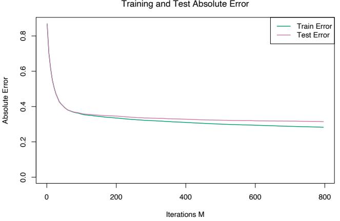
FIGURE 10.13. Average-absolute error as a function of number of iterations for the California housing data.

Figure 10.14 displays the relative variable importances for each of the eight predictor variables. Not surprisingly, median income in the neighborhood is the most relevant predictor. Longitude, latitude, and average occupancy all have roughly half the relevance of income, whereas the others are somewhat less influential.

Figure 10.15 shows single-variable partial dependence plots on the most relevant nonlocation predictors. Note that the plots are not strictly smooth. This is a consequence of using tree-based models. Decision trees produce discontinuous piecewise constant models (10.25). This carries over to sums of trees (10.28), with of course many more pieces. Unlike most of the methods discussed in this book, there is no smoothness constraint imposed on the result. Arbitrarily sharp discontinuities can be modeled. The fact that these curves generally exhibit a smooth trend is because that is what is estimated to best predict the response for this problem. This is often the case.

The hash marks at the base of each plot delineate the deciles of the data distribution of the corresponding variables. Note that here the data density is lower near the edges, especially for larger values. This causes the curves to be somewhat less well determined in those regions. The vertical scales of the plots are the same, and give a visual comparison of the relative importance of the different variables.

The partial dependence of median house value on median income is monotonic increasing, being nearly linear over the main body of data. House value is generally monotonic decreasing with increasing average occupancy, except perhaps for average occupancy rates less than one. Median house

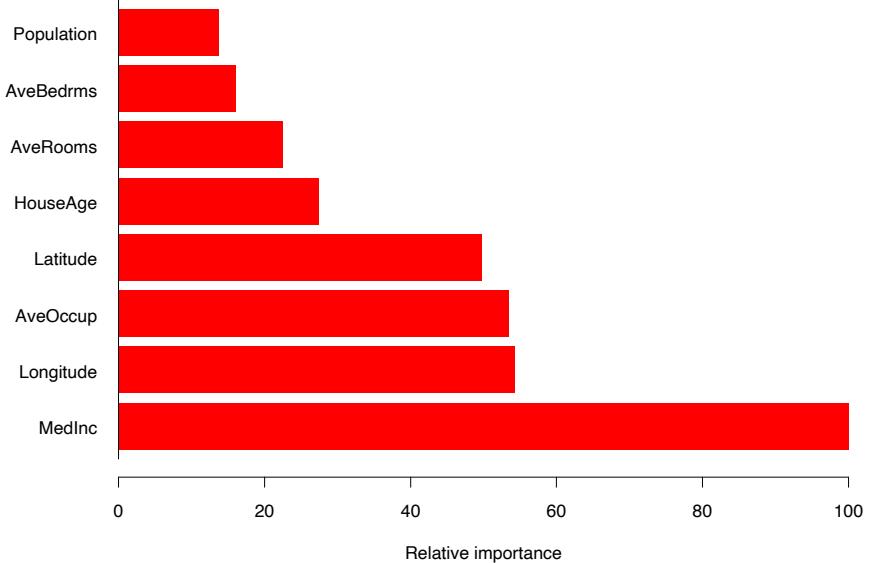
FIGURE 10.14. Relative importance of the predictors for the California housing data.

value has a nonmonotonic partial dependence on average number of rooms. It has a minimum at approximately three rooms and is increasing both for smaller and larger values.

Median house value is seen to have a very weak partial dependence on house age that is inconsistent with its importance ranking (Figure 10.14). This suggests that this weak main effect may be masking stronger interaction effects with other variables. Figure 10.16 shows the two-variable partial dependence of housing value on joint values of median age and average occupancy. An interaction between these two variables is apparent. For values of average occupancy greater than two, house value is nearly independent of median age, whereas for values less than two there is a strong dependence on age.

Figure 10.17 shows the two-variable partial dependence of the fitted model on joint values of longitude and latitude, displayed as a shaded contour plot. There is clearly a very strong dependence of median house value on the neighborhood location in California. Note that Figure 10.17 is not a plot of house value versus location ignoring the effects of the other predictors (10.49). Like all partial dependence plots, it represents the effect of location after accounting for the effects of the other neighborhood and house attributes (10.47). It can be viewed as representing an extra premium one pays for location. This premium is seen to be relatively large near the Pacific coast especially in the Bay Area and Los Angeles–San Diego re-

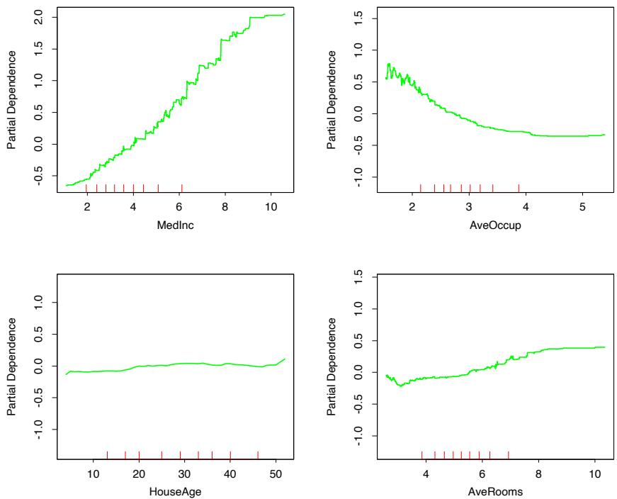
FIGURE 10.15. Partial dependence of housing value on the nonlocation variables for the California housing data. The red ticks at the base of the plot are deciles of the input variables.

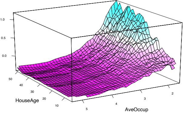
FIGURE 10.16. Partial dependence of house value on median age and average occupancy. There appears to be a strong interaction effect between these two variables.

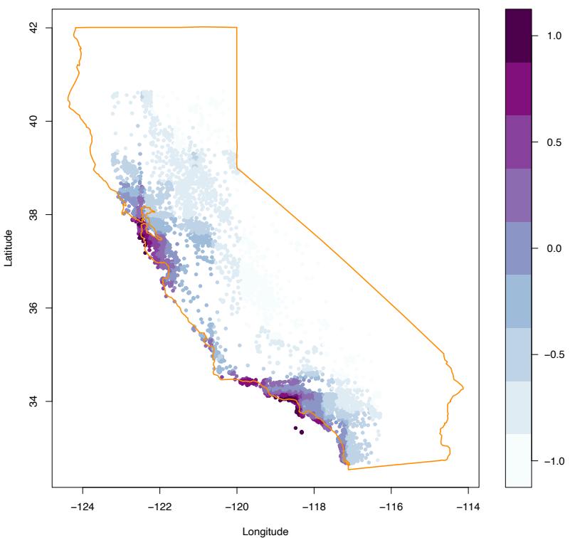
FIGURE 10.17. Partial dependence of median house value on location in California. One unit is $100, 000, at 1990 prices, and the values plotted are relative to the overall median of $180, 000.

gions. In the northern, central valley, and southeastern desert regions of California, location costs considerably less.

10.14.2 New Zealand Fish

Plant and animal ecologists use regression models to predict species presence, abundance and richness as a function of environmental variables. Although for many years simple linear and parametric models were popular, recent literature shows increasing interest in more sophisticated models such as generalized additive models (Section 9.1, GAM), multivariate adaptive regression splines (Section 9.4, MARS) and boosted regression trees (Leathwick et al., 2005; Leathwick et al., 2006). Here we model the

376 10. Boosting and Additive Trees

presence and abundance of the Black Oreo Dory, a marine fish found in the oceanic waters around New Zealand.³

Figure 10.18 shows the locations of 17,000 trawls (deep-water net fishing, with a maximum depth of 2km), and the red points indicate those 2353 trawls for which the Black Oreo was present, one of over a hundred species regularly recorded. The catch size in kg for each species was recorded for each trawl. Along with the species catch, a number of environmental measurements are available for each trawl. These include the average depth of the trawl (AvgDepth), and the temperature and salinity of the water. Since the latter two are strongly correlated with depth, Leathwick et al. (2006) derived instead TempResid and SalResid, the residuals obtained when these two measures are adjusted for depth (via separate non-parametric regressions). SSTGrad is a measure of the gradient of the sea surface temperature, and Chla is a broad indicator of ecosytem productivity via satellite-image measurements. SusPartMatter provides a measure of suspended particulate matter, particularly in coastal waters, and is also satellite derived.

The goal of this analysis is to estimate the probability of finding Black Oreo in a trawl, as well as the expected catch size, standardized to take into account the effects of variation in trawl speed and distance, as well as the mesh size of the trawl net. The authors used logistic regression for estimating the probability. For the catch size, it might seem natural to assume a Poisson distribution and model the log of the mean count, but this is often not appropriate because of the excessive number of zeros. Although specialized approaches have been developed, such as the zeroinflated Poisson (Lambert, 1992), they chose a simpler approach. If Y is the (non-negative) catch size,

\[\operatorname{E}(Y|X) = \operatorname{E}(Y|Y>0, X) \cdot \Pr(Y>0|X). \tag{10.54}\]

The second term is estimated by the logistic regression, and the first term can be estimated using only the 2353 trawls with a positive catch.

For the logistic regression the authors used a gradient boosted model (GBM)⁴ with binomial deviance loss function, depth-10 trees, and a shrinkage factor ν = 0.025. For the positive-catch regression, they modeled log(Y ) using a GBM with squared-error loss (also depth-10 trees, but ν = 0.01), and un-logged the predictions. In both cases they used 10-fold cross-validation for selecting the number of terms, as well as the shrinkage factor.

³The models, data, and maps shown here were kindly provided by Dr John Leathwick of the National Institute of Water and Atmospheric Research in New Zealand, and Dr Jane Elith, School of Botany, University of Melbourne. The collection of the research trawl data took place from 1979–2005, and was funded by the New Zealand Ministry of Fisheries.

⁴Version 1.5-7 of package gbm in R, ver. 2.2.0.

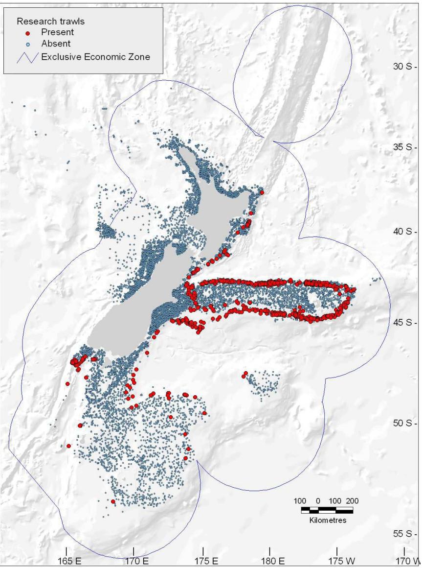
FIGURE 10.18. Map of New Zealand and its surrounding exclusive economic zone, showing the locations of 17,000 trawls (small blue dots) taken between 1979 and 2005. The red points indicate trawls for which the species Black Oreo Dory were present.

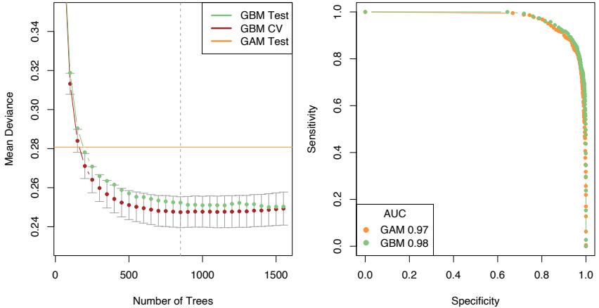
FIGURE 10.19. The left panel shows the mean deviance as a function of the number of trees for the GBM logistic regression model fit to the presence/absence data. Shown are 10-fold cross-validation on the training data (and 1 × s.e. bars), and test deviance on the test data. Also shown for comparison is the test deviance using a GAM model with 8 df for each term. The right panel shows ROC curves on the test data for the chosen GBM model (vertical line in left plot) and the GAM model.

Figure 10.19 (left panel) shows the mean binomial deviance for the sequence of GBM models, both for 10-fold CV and test data. There is a modest improvement over the performance of a GAM model, fit using smoothing splines with 8 degrees-of-freedom (df) per term. The right panel shows the ROC curves (see Section 9.2.5) for both models, which measures predictive performance. From this point of view, the performance looks very similar, with GBM perhaps having a slight edge as summarized by the AUC (area under the curve). At the point of equal sensitivity/specificity, GBM achieves 91%, and GAM 90%.

Figure 10.20 summarizes the contributions of the variables in the logistic GBM fit. We see that there is a well-defined depth range over which Black Oreo are caught, with much more frequent capture in colder waters. We do not give details of the quantitative catch model; the important variables were much the same.

All the predictors used in these models are available on a fine geographical grid; in fact they were derived from environmental atlases, satellite images and the like—see Leathwick et al. (2006) for details. This also means that predictions can be made on this grid, and imported into GIS mapping systems. Figure 10.21 shows prediction maps for both presence and catch size, with both standardized to a common set of trawl conditions; since the predictors vary in a continuous fashion with geographical location, so do the predictions.

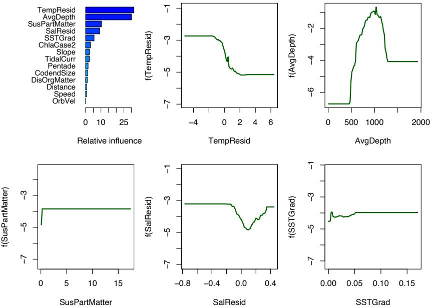
FIGURE 10.20. The top-left panel shows the relative influence computed from the GBM logistic regression model. The remaining panels show the partial dependence plots for the leading five variables, all plotted on the same scale for comparison.

Because of their ability to model interactions and automatically select variables, as well as robustness to outliers and missing data, GBM models are rapidly gaining popularity in this data-rich and enthusiastic community.

10.14.3 Demographics Data

In this section we illustrate gradient boosting on a multiclass classification problem, using MART. The data come from 9243 questionnaires filled out by shopping mall customers in the San Francisco Bay Area (Impact Resources, Inc., Columbus, OH). Among the questions are 14 concerning demographics. For this illustration the goal is to predict occupation using the other 13 variables as predictors, and hence identify demographic variables that discriminate between different occupational categories. We randomly divided the data into a training set (80%) and test set (20%), and used J = 6 node trees with a learning rate ν = 0.1.

Figure 10.22 shows the K = 9 occupation class values along with their corresponding error rates. The overall error rate is 42.5%, which can be compared to the null rate of 69% obtained by predicting the most numerous

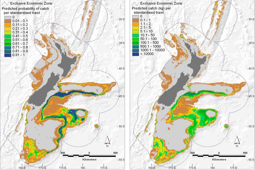
FIGURE 10.21. Geological prediction maps of the presence probability (left map) and catch size (right map) obtained from the gradient boosted models.

class Prof/Man (Professional/Managerial). The four best predicted classes are seen to be Retired, Student, Prof/Man, and Homemaker.

Figure 10.23 shows the relative predictor variable importances as averaged over all classes (10.46). Figure 10.24 displays the individual relative importance distributions (10.45) for each of the four best predicted classes. One sees that the most relevant predictors are generally different for each respective class. An exception is age which is among the three most relevant for predicting Retired, Student, and Prof/Man.

Figure 10.25 shows the partial dependence of the log-odds (10.52) on age for these three classes. The abscissa values are ordered codes for respective equally spaced age intervals. One sees that after accounting for the contributions of the other variables, the odds of being retired are higher for older people, whereas the opposite is the case for being a student. The odds of being professional/managerial are highest for middle-aged people. These results are of course not surprising. They illustrate that inspecting partial dependences separately for each class can lead to sensible results.

Bibliographic Notes

Schapire (1990) developed the first simple boosting procedure in the PAC learning framework (Valiant, 1984; Kearns and Vazirani, 1994). Schapire

Overall Error Rate = 0.425

FIGURE 10.22. Error rate for each occupation in the demographics data.

FIGURE 10.23. Relative importance of the predictors as averaged over all classes for the demographics data.

FIGURE 10.24. Predictor variable importances separately for each of the four classes with lowest error rate for the demographics data.

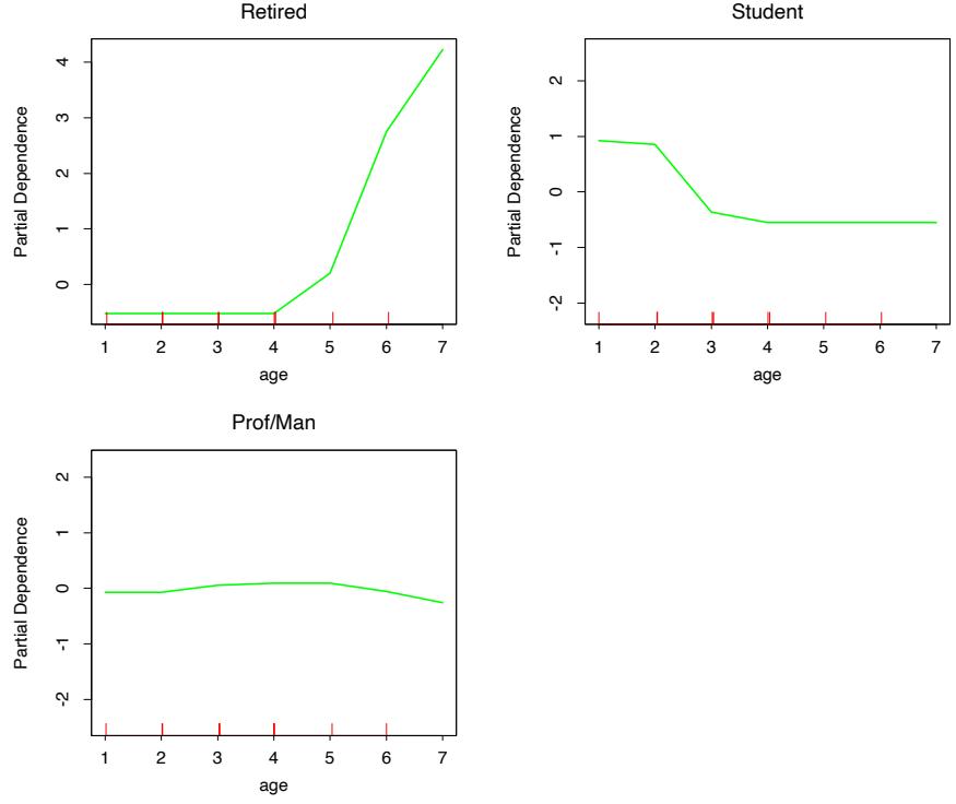
FIGURE 10.25. Partial dependence of the odds of three different occupations on age, for the demographics data.

showed that a weak learner could always improve its performance by training two additional classifiers on filtered versions of the input data stream. A weak learner is an algorithm for producing a two-class classifier with performance guaranteed (with high probability) to be significantly better than a coin-flip. After learning an initial classifier G¹ on the first N training points,

• G² is learned on a new sample of N points, half of which are misclassified by G1;
• G³ is learned on N points for which G¹ and G² disagree;
• the boosted classifier is G^B = majority vote(G1, G2, G3).

Schapire’s “Strength of Weak Learnability” theorem proves that G^B has improved performance over G1.

Freund (1995) proposed a “boost by majority” variation which combined many weak learners simultaneously and improved the performance of the simple boosting algorithm of Schapire. The theory supporting both of these

384 10. Boosting and Additive Trees

algorithms requires the weak learner to produce a classifier with a fixed error rate. This led to the more adaptive and realistic AdaBoost (Freund and Schapire, 1996a) and its offspring, where this assumption was dropped.

Freund and Schapire (1996a) and Schapire and Singer (1999) provide some theory to support their algorithms, in the form of upper bounds on generalization error. This theory has evolved in the computational learning community, initially based on the concepts of PAC learning. Other theories attempting to explain boosting come from game theory (Freund and Schapire, 1996b; Breiman, 1999; Breiman, 1998), and VC theory (Schapire et al., 1998). The bounds and the theory associated with the AdaBoost algorithms are interesting, but tend to be too loose to be of practical importance. In practice, boosting achieves results far more impressive than the bounds would imply. Schapire (2002) and Meir and R¨atsch (2003) give useful overviews more recent than the first edition of this book.

Friedman et al. (2000) and Friedman (2001) form the basis for our exposition in this chapter. Friedman et al. (2000) analyze AdaBoost statistically, derive the exponential criterion, and show that it estimates the log-odds of the class probability. They propose additive tree models, the right-sized trees and ANOVA representation of Section 10.11, and the multiclass logit formulation. Friedman (2001) developed gradient boosting and shrinkage for classification and regression, while Friedman (1999) explored stochastic variants of boosting. Mason et al. (2000) also embraced a gradient approach to boosting. As the published discussions of Friedman et al. (2000) shows, there is some controversy about how and why boosting works.

Since the publication of the first edition of this book, these debates have continued, and spread into the statistical community with a series of papers on consistency of boosting (Jiang, 2004; Lugosi and Vayatis, 2004; Zhang and Yu, 2005; Bartlett and Traskin, 2007). Mease and Wyner (2008), through a series of simulation examples, challenge some of our interpretations of boosting; our response (Friedman et al., 2008a) puts most of these objections to rest. A recent survey by B¨uhlmann and Hothorn (2007) supports our approach to boosting.

Exercises

Ex. 10.1 Derive expression (10.12) for the update parameter in AdaBoost.

Ex. 10.2 Prove result (10.16), that is, the minimizer of the population version of the AdaBoost criterion, is one-half of the log odds.

Ex. 10.3 Show that the marginal average (10.47) recovers additive and multiplicative functions (10.50) and (10.51), while the conditional expectation (10.49) does not.

Ex. 10.4

• 1. Write a program implementing AdaBoost with trees.
• 2. Redo the computations for the example of Figure 10.2. Plot the training error as well as test error, and discuss its behavior.
• 3. Investigate the number of iterations needed to make the test error finally start to rise.
• 4. Change the setup of this example as follows: define two classes, with the features in Class 1 being X1, X2,…,X10, standard independent Gaussian variates. In Class 2, the features X1, X2,…,X¹⁰ are also standard independent Gaussian, but conditioned on the event # ^j X^{2 j} > 12. Now the classes have significant overlap in feature space. Repeat the AdaBoost experiments as in Figure 10.2 and discuss the results.

Ex. 10.5 Multiclass exponential loss (Zhu et al., 2005). For a K-class classification problem, consider the coding Y = (Y1,…,YK)^T with

\[Y\_k = \begin{cases} 1, & \text{if } G = \mathcal{G}\_k \\ -\frac{1}{K-1}, & \text{otherwise.} \end{cases} \tag{10.55}\]

Let f = (f1,…,fK)^T with #^{K k}=1 f^k = 0, and define

\[L(Y, f) = \exp\left(-\frac{1}{K}Y^T f\right). \tag{10.56}\]

• 1. Using Lagrange multipliers, derive the population minimizer f ^∗ of E(Y,f), subject to the zero-sum constraint, and relate these to the class probabilities.
• 2. Show that a multiclass boosting using this loss function leads to a reweighting algorithm similar to Adaboost, as in Section 10.4.

Ex. 10.6 McNemar test (Agresti, 1996). We report the test error rates on the spam data to be 5.5% for a generalized additive model (GAM), and 4.5% for gradient boosting (GBM), with a test sample of size 1536.

1. Show that the standard error of these estimates is about 0.6%.

Since the same test data are used for both methods, the error rates are correlated, and we cannot perform a two-sample t-test. We can compare the methods directly on each test observation, leading to the summary

	GBM
GAM	Correct	Error
Correct	1434	18
Error	33	51

The McNemar test focuses on the discordant errors, 33 vs. 18.

2. Conduct a test to show that GAM makes significantly more errors than gradient boosting, with a two-sided p-value of 0.036.

Ex. 10.7 Derive expression (10.32).

Ex. 10.8 Consider a K-class problem where the targets yik are coded as 1 if observation i is in class k and zero otherwise. Suppose we have a current model fk(x), k = 1,…,K, with #^{K k}=1 fk(x) = 0 (see (10.21) in Section 10.6). We wish to update the model for observations in a region R in predictor space, by adding constants fk(x) + γk, with γ^K = 0.

• 1. Write down the multinomial log-likelihood for this problem, and its first and second derivatives.
• 2. Using only the diagonal of the Hessian matrix in (1), and starting from γ^k = 0 ∀k, show that a one-step approximate Newton update for γ^k is

\[\gamma\_k^1 = \frac{\sum\_{x\_i \in R} (y\_{ik} - p\_{ik})}{\sum\_{x\_i \in R} p\_{ik}(1 - p\_{ik})}, \ k = 1, \dots, K - 1,\tag{10.57}\]

where pik = exp(fk(xi))/( #^{K ℓ}=1 fℓ(xi)).

3. We prefer our update to sum to zero, as the current model does. Using symmetry arguments, show that

\[\hat{\gamma}\_k = \frac{K-1}{K} (\gamma\_k^1 - \frac{1}{K} \sum\_{\ell=1}^K \gamma\_\ell^1), \ k = 1, \dots, K \tag{10.58}\]

is an appropriate update, where γ^{1 k} is defined as in (10.57) for all k = 1,…,K.

Ex. 10.9 Consider a K-class problem where the targets yik are coded as 1 if observation i is in class k and zero otherwise. Using the multinomial deviance loss function (10.22) and the symmetric logistic transform, use the arguments leading to the gradient boosting Algorithm 10.3 to derive Algorithm 10.4. Hint: See exercise 10.8 for step 2(b)iii.

Ex. 10.10 Show that for K = 2 class classification, only one tree needs to be grown at each gradient-boosting iteration.

Ex. 10.11 Show how to compute the partial dependence function f^S (X^S ) in (10.47) efficiently.

Ex. 10.12 Referring to (10.49), let S = {1} and C = {2}, with f(X1, X2) = X1. Assume X¹ and X² are bivariate Gaussian, each with mean zero, variance one, and E(X1, X2) = ρ. Show that E(f(X1, X2|X2) = ρX2, even though f is not a function of X2.

Algorithm 10.4 Gradient Boosting for K-class Classification.

• 1. Initialize fk0(x)=0, k = 1, 2,…,K.
• 2. For m=1 to M:
  • 1. Set

\[p\_k(x) = \frac{e^{f\_k(x)}}{\sum\_{\ell=1}^K e^{f\_\ell(x)}}, \ k = 1, 2, \dots, K.\]

• 2. For k = 1 to K:
  • 1. Compute rikm = yik − pk(xi), i = 1, 2,…,N.
  • 2. Fit a regression tree to the targets rikm, i = 1, 2,…,N, giving terminal regions Rjkm, j = 1, 2,…,Jm.
  • 3. Compute

\[\gamma\_{jkm} = \frac{K-1}{K} \frac{\sum\_{x\_i \in R\_{jkm}} r\_{ikm}}{\sum\_{x\_i \in R\_{jkm}} |r\_{ikm}|(1 - |r\_{ikm}|)}, \; j = 1, 2, \dots, J\_m.\]

4. Update fkm(x) = fk,m−1(x) + #^{Jm j}=1 γjkmI(x ∈ Rjkm).

3. Output ˆfk(x) = fkM(x), k = 1, 2,…,K.

388 10. Boosting and Additive Trees

This is page 389 Printer: Opaque this

11 Neural Networks

11.1 Introduction

In this chapter we describe a class of learning methods that was developed separately in different fields—statistics and artificial intelligence—based on essentially identical models. The central idea is to extract linear combinations of the inputs as derived features, and then model the target as a nonlinear function of these features. The result is a powerful learning method, with widespread applications in many fields. We first discuss the projection pursuit model, which evolved in the domain of semiparametric statistics and smoothing. The rest of the chapter is devoted to neural network models.

11.2 Projection Pursuit Regression

As in our generic supervised learning problem, assume we have an input vector X with p components, and a target Y . Let ωm, m = 1, 2,…,M, be unit p-vectors of unknown parameters. The projection pursuit regression (PPR) model has the form

\[f(X) = \sum\_{m=1}^{M} g\_m(\omega\_m^T X). \tag{11.1}\]

This is an additive model, but in the derived features V^m = ω^{T m}X rather than the inputs themselves. The functions g^m are unspecified and are esti-

FIGURE 11.1. Perspective plots of two ridge functions. (Left:) g(V )=1/[1 + exp(−5(V − 0.5))], where V = (X¹ + X2)/ ^√2. (Right:) g(V )=(V + 0.1) sin(1/(V /3+0.1)), where V = X1.

mated along with the directions ω^m using some flexible smoothing method (see below).

The function gm(ω^{T m}X) is called a ridge function in IR^p. It varies only in the direction defined by the vector ωm. The scalar variable V^m = ω^{T m}X is the projection of X onto the unit vector ωm, and we seek ω^m so that the model fits well, hence the name “projection pursuit.” Figure 11.1 shows some examples of ridge functions. In the example on the left ω = (1/ ^√2)(1, 1)^T , so that the function only varies in the direction X¹ + X2. In the example on the right, ω = (1, 0).

The PPR model (11.1) is very general, since the operation of forming nonlinear functions of linear combinations generates a surprisingly large class of models. For example, the product X¹ · X² can be written as [(X¹ + ^X2)^{2 −} (X^{1 − X}2)²]/4, and higher-order products can be represented similarly.

In fact, if M is taken arbitrarily large, for appropriate choice of g^m the PPR model can approximate any continuous function in IR^p arbitrarily well. Such a class of models is called a universal approximator. However this generality comes at a price. Interpretation of the fitted model is usually difficult, because each input enters into the model in a complex and multifaceted way. As a result, the PPR model is most useful for prediction, and not very useful for producing an understandable model for the data. The M = 1 model, known as the single index model in econometrics, is an exception. It is slightly more general than the linear regression model, and offers a similar interpretation.

How do we fit a PPR model, given training data (xi, yi), i = 1, 2,…,N? We seek the approximate minimizers of the error function

\[\sum\_{i=1}^{N} \left[ y\_i - \sum\_{m=1}^{M} g\_m(\omega\_m^T x\_i) \right]^2 \tag{11.2}\]

over functions g^m and direction vectors ωm, m = 1, 2,…,M. As in other smoothing problems, we need either explicitly or implicitly to impose complexity constraints on the gm, to avoid overfit solutions.

Consider just one term (M = 1, and drop the subscript). Given the direction vector ω, we form the derived variables vⁱ = ω^T xi. Then we have a one-dimensional smoothing problem, and we can apply any scatterplot smoother, such as a smoothing spline, to obtain an estimate of g.

On the other hand, given g, we want to minimize (11.2) over ω. A Gauss– Newton search is convenient for this task. This is a quasi-Newton method, in which the part of the Hessian involving the second derivative of g is discarded. It can be simply derived as follows. Let ωold be the current estimate for ω. We write

\[g(\omega^T x\_i) \approx g(\omega\_{\text{old}}^T x\_i) + g'(\omega\_{\text{old}}^T x\_i)(\omega - \omega\_{\text{old}})^T x\_i \tag{11.3}\]

to give

\[\sum\_{i=1}^{N} \left[ y\_i - g(\boldsymbol{\omega}^T \boldsymbol{x}\_i) \right]^2 \approx \sum\_{i=1}^{N} g'(\boldsymbol{\omega}\_{\text{old}}^T \boldsymbol{x}\_i)^2 \left[ \left( \boldsymbol{\omega}\_{\text{old}}^T \boldsymbol{x}\_i + \frac{y\_i - g(\boldsymbol{\omega}\_{\text{old}}^T \boldsymbol{x}\_i)}{g'(\boldsymbol{\omega}\_{\text{old}}^T \boldsymbol{x}\_i)} \right) - \boldsymbol{\omega}^T \boldsymbol{x}\_i \right]^2 \. \tag{11.4}\]

To minimize the right-hand side, we carry out a least squares regression with target ω^T oldxi+(yi−g(ω^T oldxi))/g′ (ω^T oldxi) on the input xi, with weights g′ (ω^T oldxi)² and no intercept (bias) term. This produces the updated coefficient vector ωnew.

These two steps, estimation of g and ω, are iterated until convergence. With more than one term in the PPR model, the model is built in a forward stage-wise manner, adding a pair (ωm, gm) at each stage.

There are a number of implementation details.

• Although any smoothing method can in principle be used, it is convenient if the method provides derivatives. Local regression and smoothing splines are convenient.
• After each step the gm’s from previous steps can be readjusted using the backfitting procedure described in Chapter 9. While this may lead ultimately to fewer terms, it is not clear whether it improves prediction performance.
• Usually the ω^m are not readjusted (partly to avoid excessive computation), although in principle they could be as well.
• The number of terms M is usually estimated as part of the forward stage-wise strategy. The model building stops when the next term does not appreciably improve the fit of the model. Cross-validation can also be used to determine M.

392 Neural Networks

There are many other applications, such as density estimation (Friedman et al., 1984; Friedman, 1987), where the projection pursuit idea can be used. In particular, see the discussion of ICA in Section 14.7 and its relationship with exploratory projection pursuit. However the projection pursuit regression model has not been widely used in the field of statistics, perhaps because at the time of its introduction (1981), its computational demands exceeded the capabilities of most readily available computers. But it does represent an important intellectual advance, one that has blossomed in its reincarnation in the field of neural networks, the topic of the rest of this chapter.

11.3 Neural Networks

The term neural network has evolved to encompass a large class of models and learning methods. Here we describe the most widely used “vanilla” neural net, sometimes called the single hidden layer back-propagation network, or single layer perceptron. There has been a great deal of hype surrounding neural networks, making them seem magical and mysterious. As we make clear in this section, they are just nonlinear statistical models, much like the projection pursuit regression model discussed above.

A neural network is a two-stage regression or classification model, typically represented by a network diagram as in Figure 11.2. This network applies both to regression or classification. For regression, typically K = 1 and there is only one output unit Y¹ at the top. However, these networks can handle multiple quantitative responses in a seamless fashion, so we will deal with the general case.

For K-class classification, there are K units at the top, with the kth unit modeling the probability of class k. There are K target measurements Yk, k = 1,…,K, each being coded as a 0 − 1 variable for the kth class.

Derived features Z^m are created from linear combinations of the inputs, and then the target Y^k is modeled as a function of linear combinations of the Zm,

\[\begin{aligned} Z\_m &= \sigma(\alpha\_{0m} + \alpha\_m^T X), \ m = 1, \dots, M, \\ T\_k &= \beta\_{0k} + \beta\_k^T Z, \ k = 1, \dots, K, \\ f\_k(X) &= g\_k(T), \ k = 1, \dots, K, \end{aligned} \tag{11.5}\]

where Z = (Z1, Z2,…,ZM), and T = (T1, T2,…,TK).

The activation function σ(v) is usually chosen to be the sigmoid σ(v) = 1/(1 + e−v); see Figure 11.3 for a plot of 1/(1 + e−v). Sometimes Gaussian radial basis functions (Chapter 6) are used for the σ(v), producing what is known as a radial basis function network.

Neural network diagrams like Figure 11.2 are sometimes drawn with an additional bias unit feeding into every unit in the hidden and output layers.

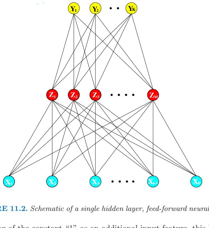
FIGURE 11.2. Schematic of a single hidden layer, feed-forward neural network.

Thinking of the constant “1” as an additional input feature, this bias unit captures the intercepts α0^m and β0^k in model (11.5).

The output function gk(T) allows a final transformation of the vector of outputs T. For regression we typically choose the identity function gk(T) = Tk. Early work in K-class classification also used the identity function, but this was later abandoned in favor of the softmax function

\[g\_k(T) = \frac{e^{T\_k}}{\sum\_{\ell=1}^K e^{T\_\ell}}.\tag{11.6}\]

This is of course exactly the transformation used in the multilogit model (Section 4.4), and produces positive estimates that sum to one. In Section 4.2 we discuss other problems with linear activation functions, in particular potentially severe masking effects.

The units in the middle of the network, computing the derived features Zm, are called hidden units because the values Z^m are not directly observed. In general there can be more than one hidden layer, as illustrated in the example at the end of this chapter. We can think of the Z^m as a basis expansion of the original inputs X; the neural network is then a standard linear model, or linear multilogit model, using these transformations as inputs. There is, however, an important enhancement over the basisexpansion techniques discussed in Chapter 5; here the parameters of the basis functions are learned from the data.

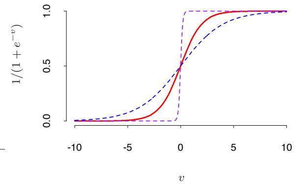
FIGURE 11.3. Plot of the sigmoid function σ(v)=1/(1+exp(−v)) (red curve), commonly used in the hidden layer of a neural network. Included are σ(sv) for s = ^{1 2} (blue curve) and s = 10 (purple curve). The scale parameter s controls the activation rate, and we can see that large s amounts to a hard activation at v = 0. Note that σ(s(v − v0)) shifts the activation threshold from 0 to v0.

Notice that if σ is the identity function, then the entire model collapses to a linear model in the inputs. Hence a neural network can be thought of as a nonlinear generalization of the linear model, both for regression and classification. By introducing the nonlinear transformation σ, it greatly enlarges the class of linear models. In Figure 11.3 we see that the rate of activation of the sigmoid depends on the norm of αm, and if ∥αm∥ is very small, the unit will indeed be operating in the linear part of its activation function.

Notice also that the neural network model with one hidden layer has exactly the same form as the projection pursuit model described above. The difference is that the PPR model uses nonparametric functions gm(v), while the neural network uses a far simpler function based on σ(v), with three free parameters in its argument. In detail, viewing the neural network model as a PPR model, we identify

\[\begin{aligned} g\_m(\omega\_m^T X) &= \beta\_m \sigma(\alpha\_{0m} + \alpha\_m^T X) \\ &= \beta\_m \sigma(\alpha\_{0m} + ||\alpha\_m||(\omega\_m^T X)), \end{aligned} \tag{11.7}\]

where ω^m = αm/∥αm∥ is the mth unit-vector. Since σβ,α0,s(v) = βσ(α⁰ + sv) has lower complexity than a more general nonparametric g(v), it is not surprising that a neural network might use 20 or 100 such functions, while the PPR model typically uses fewer terms (M = 5 or 10, for example).

Finally, we note that the name “neural networks” derives from the fact that they were first developed as models for the human brain. Each unit represents a neuron, and the connections (links in Figure 11.2) represent synapses. In early models, the neurons fired when the total signal passed to that unit exceeded a certain threshold. In the model above, this corresponds to use of a step function for σ(Z) and gm(T). Later the neural network was recognized as a useful tool for nonlinear statistical modeling, and for this purpose the step function is not smooth enough for optimization. Hence the step function was replaced by a smoother threshold function, the sigmoid in Figure 11.3.

11.4 Fitting Neural Networks

The neural network model has unknown parameters, often called weights, and we seek values for them that make the model fit the training data well. We denote the complete set of weights by θ, which consists of

\[\begin{aligned} \{\alpha\_{0m}, \alpha\_m; \ m &= 1, 2, \dots, M\} & &M(p+1) \text{ weights},\\ \{\beta\_{0k}, \beta\_k; \ k &= 1, 2, \dots, K\} & &K(M+1) \text{ weights}. \end{aligned} \tag{11.8}\]

For regression, we use sum-of-squared errors as our measure of fit (error function)

\[R(\theta) = \sum\_{k=1}^{K} \sum\_{i=1}^{N} (y\_{ik} - f\_k(x\_i))^2. \tag{11.9}\]

For classification we use either squared error or cross-entropy (deviance):

\[R(\theta) = -\sum\_{i=1}^{N} \sum\_{k=1}^{K} y\_{ik} \log f\_k(x\_i),\tag{11.10}\]

and the corresponding classifier is G(x) = argmaxkfk(x). With the softmax activation function and the cross-entropy error function, the neural network model is exactly a linear logistic regression model in the hidden units, and all the parameters are estimated by maximum likelihood.

Typically we don’t want the global minimizer of R(θ), as this is likely to be an overfit solution. Instead some regularization is needed: this is achieved directly through a penalty term, or indirectly by early stopping. Details are given in the next section.

The generic approach to minimizing R(θ) is by gradient descent, called back-propagation in this setting. Because of the compositional form of the model, the gradient can be easily derived using the chain rule for differentiation. This can be computed by a forward and backward sweep over the network, keeping track only of quantities local to each unit.

396 Neural Networks

Here is back-propagation in detail for squared error loss. Let zmi = σ(α0^m + α^{T m}xi), from (11.5) and let zⁱ = (z1i, z2i,…,zM i). Then we have

\[\begin{aligned} R(\theta) & \equiv \sum\_{i=1}^{N} R\_i \\ &= \sum\_{i=1}^{N} \sum\_{k=1}^{K} (y\_{ik} - f\_k(x\_i))^2, \end{aligned} \tag{11.11}\]

with derivatives

\[\begin{split} \frac{\partial R\_i}{\partial \beta\_{km}} &= -2(y\_{ik} - f\_k(x\_i))g\_k'(\beta\_k^T z\_i)z\_{mi}, \\ \frac{\partial R\_i}{\partial \alpha\_{m\ell}} &= -\sum\_{k=1}^K 2(y\_{ik} - f\_k(x\_i))g\_k'(\beta\_k^T z\_i)\beta\_{km}\sigma'(\alpha\_m^T x\_i)x\_{i\ell}. \end{split} \tag{11.12}\]

Given these derivatives, a gradient descent update at the (r + 1)st iteration has the form

\[\begin{split} \beta\_{km}^{(r+1)} &= \beta\_{km}^{(r)} - \gamma\_r \sum\_{i=1}^{N} \frac{\partial R\_i}{\partial \beta\_{km}^{(r)}}, \\ \alpha\_{m\ell}^{(r+1)} &= \alpha\_{m\ell}^{(r)} - \gamma\_r \sum\_{i=1}^{N} \frac{\partial R\_i}{\partial \alpha\_{m\ell}^{(r)}}, \end{split} \tag{11.13}\]

where γ^r is the learning rate, discussed below.

Now write (11.12) as

\[\begin{aligned} \frac{\partial R\_i}{\partial \beta\_{km}} &= \delta\_{ki} z\_{mi}, \\ \frac{\partial R\_i}{\partial \alpha\_{m\ell}} &= s\_{mi} x\_{i\ell}. \end{aligned} \tag{11.14}\]

The quantities δki and smi are “errors” from the current model at the output and hidden layer units, respectively. From their definitions, these errors satisfy

\[s\_{mi} = \sigma'(\alpha\_m^T x\_i) \sum\_{k=1}^K \beta\_{km} \delta\_{ki},\tag{11.15}\]

known as the back-propagation equations. Using this, the updates in (11.13) can be implemented with a two-pass algorithm. In the forward pass, the current weights are fixed and the predicted values ˆfk(xi) are computed from formula (11.5). In the backward pass, the errors δki are computed, and then back-propagated via (11.15) to give the errors smi. Both sets of errors are then used to compute the gradients for the updates in (11.13), via (11.14).

This two-pass procedure is what is known as back-propagation. It has also been called the delta rule (Widrow and Hoff, 1960). The computational components for cross-entropy have the same form as those for the sum of squares error function, and are derived in Exercise 11.3.

The advantages of back-propagation are its simple, local nature. In the back propagation algorithm, each hidden unit passes and receives information only to and from units that share a connection. Hence it can be implemented efficiently on a parallel architecture computer.

The updates in (11.13) are a kind of batch learning, with the parameter updates being a sum over all of the training cases. Learning can also be carried out online—processing each observation one at a time, updating the gradient after each training case, and cycling through the training cases many times. In this case, the sums in equations (11.13) are replaced by a single summand. A training epoch refers to one sweep through the entire training set. Online training allows the network to handle very large training sets, and also to update the weights as new observations come in.

The learning rate γ^r for batch learning is usually taken to be a constant, and can also be optimized by a line search that minimizes the error function at each update. With online learning γ^r should decrease to zero as the iteration r → ∞. This learning is a form of stochastic approximation (Robbins and Munro, 1951); results in this field ensure convergence if ^{γr →} 0, # ^{r γr = ∞}, and # ^r γ^{2 r} < ∞ (satisfied, for example, by γ^r = 1/r).

Back-propagation can be very slow, and for that reason is usually not the method of choice. Second-order techniques such as Newton’s method are not attractive here, because the second derivative matrix of R (the Hessian) can be very large. Better approaches to fitting include conjugate gradients and variable metric methods. These avoid explicit computation of the second derivative matrix while still providing faster convergence.

11.5 Some Issues in Training Neural Networks

There is quite an art in training neural networks. The model is generally overparametrized, and the optimization problem is nonconvex and unstable unless certain guidelines are followed. In this section we summarize some of the important issues.

11.5.1 Starting Values

Note that if the weights are near zero, then the operative part of the sigmoid (Figure 11.3) is roughly linear, and hence the neural network collapses into an approximately linear model (Exercise 11.2). Usually starting values for weights are chosen to be random values near zero. Hence the model starts out nearly linear, and becomes nonlinear as the weights increase. Individual

398 Neural Networks

units localize to directions and introduce nonlinearities where needed. Use of exact zero weights leads to zero derivatives and perfect symmetry, and the algorithm never moves. Starting instead with large weights often leads to poor solutions.

11.5.2 Overfitting

Often neural networks have too many weights and will overfit the data at the global minimum of R. In early developments of neural networks, either by design or by accident, an early stopping rule was used to avoid overfitting. Here we train the model only for a while, and stop well before we approach the global minimum. Since the weights start at a highly regularized (linear) solution, this has the effect of shrinking the final model toward a linear model. A validation dataset is useful for determining when to stop, since we expect the validation error to start increasing.

A more explicit method for regularization is weight decay, which is analogous to ridge regression used for linear models (Section 3.4.1). We add a penalty to the error function R(θ) + λJ(θ), where

\[J(\theta) = \sum\_{km} \beta\_{km}^2 + \sum\_{m\ell} \alpha\_{m\ell}^2 \tag{11.16}\]

and λ ≥ 0 is a tuning parameter. Larger values of λ will tend to shrink the weights toward zero: typically cross-validation is used to estimate λ. The effect of the penalty is to simply add terms 2βkm and 2αm^ℓ to the respective gradient expressions (11.13). Other forms for the penalty have been proposed, for example,

\[J(\theta) = \sum\_{km} \frac{\beta\_{km}^2}{1 + \beta\_{km}^2} + \sum\_{m\ell} \frac{\alpha\_{m\ell}^2}{1 + \alpha\_{m\ell}^2},\tag{11.17}\]

known as the weight elimination penalty. This has the effect of shrinking smaller weights more than (11.16) does.

Figure 11.4 shows the result of training a neural network with ten hidden units, without weight decay (upper panel) and with weight decay (lower panel), to the mixture example of Chapter 2. Weight decay has clearly improved the prediction. Figure 11.5 shows heat maps of the estimated weights from the training (grayscale versions of these are called Hinton diagrams.) We see that weight decay has dampened the weights in both layers: the resulting weights are spread fairly evenly over the ten hidden units.

11.5.3 Scaling of the Inputs

Since the scaling of the inputs determines the effective scaling of the weights in the bottom layer, it can have a large effect on the quality of the final

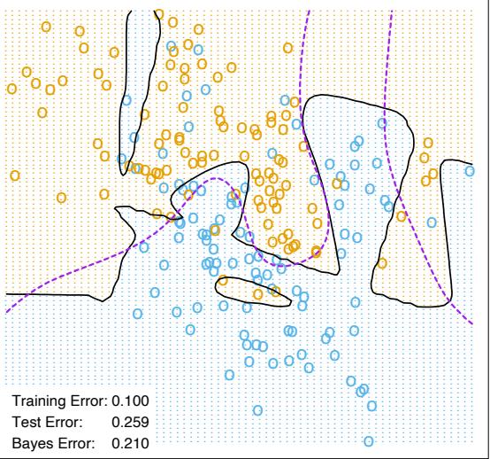
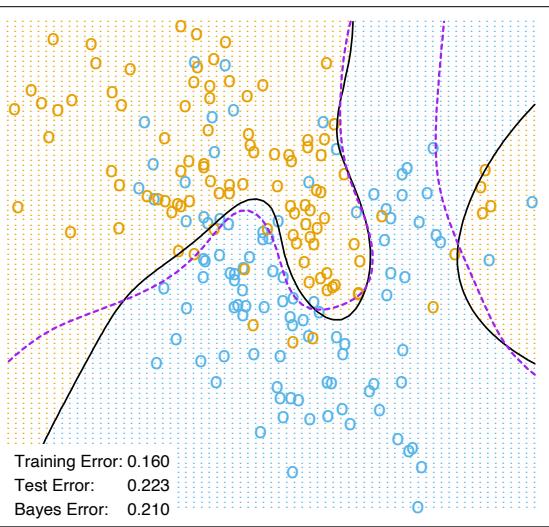
400 Neural Networks

FIGURE 11.5. Heat maps of the estimated weights from the training of neural networks from Figure 11.4. The display ranges from bright green (negative) to bright red (positive).

solution. At the outset it is best to standardize all inputs to have mean zero and standard deviation one. This ensures all inputs are treated equally in the regularization process, and allows one to choose a meaningful range for the random starting weights. With standardized inputs, it is typical to take random uniform weights over the range [−0.7, +0.7].

11.5.4 Number of Hidden Units and Layers

Generally speaking it is better to have too many hidden units than too few. With too few hidden units, the model might not have enough flexibility to capture the nonlinearities in the data; with too many hidden units, the extra weights can be shrunk toward zero if appropriate regularization is used. Typically the number of hidden units is somewhere in the range of 5 to 100, with the number increasing with the number of inputs and number of training cases. It is most common to put down a reasonably large number of units and train them with regularization. Some researchers use cross-validation to estimate the optimal number, but this seems unnecessary if cross-validation is used to estimate the regularization parameter. Choice of the number of hidden layers is guided by background knowledge and experimentation. Each layer extracts features of the input for regression or classification. Use of multiple hidden layers allows construction of hierarchical features at different levels of resolution. An example of the effective use of multiple layers is given in Section 11.6.

11.5.5 Multiple Minima

The error function R(θ) is nonconvex, possessing many local minima. As a result, the final solution obtained is quite dependent on the choice of starting weights. One must at least try a number of random starting configurations, and choose the solution giving lowest (penalized) error. Probably a better approach is to use the average predictions over the collection of networks as the final prediction (Ripley, 1996). This is preferable to averaging the weights, since the nonlinearity of the model implies that this averaged solution could be quite poor. Another approach is via bagging, which averages the predictions of networks training from randomly perturbed versions of the training data. This is described in Section 8.7.

11.6 Example: Simulated Data

We generated data from two additive error models Y = f(X) + ε:

\[\begin{aligned} \text{Sum of signals:} \ Y &= \ \sigma(a\_1^T X) + \sigma(a\_2^T X) + \varepsilon\_1; \\ \text{Radial:} \ Y &= \ \prod\_{m=1}^{10} \phi(X\_m) + \varepsilon\_2. \end{aligned}\]

Here X^T = (X1, X2,…,Xp), each X^j being a standard Gaussian variate, with p = 2 in the first model, and p = 10 in the second.

For the sigmoid model, a¹ = (3, 3), a² = (3, −3); for the radial model, ^φ(t) = (1/2π)¹/² exp(−^{t 2}/2). Both ε¹ and ε² are Gaussian errors, with variance chosen so that the signal-to-noise ratio

\[\frac{\text{Var}(\mathcal{E}(Y|X))}{\text{Var}(Y - \mathcal{E}(Y|X))} = \frac{\text{Var}(f(X))}{\text{Var}(\varepsilon)}\tag{11.18}\]

is 4 in both models. We took a training sample of size 100 and a test sample of size 10, 000. We fit neural networks with weight decay and various numbers of hidden units, and recorded the average test error ETest(^{Y − ˆ}f(X))² for each of 10 random starting weights. Only one training set was generated, but the results are typical for an “average” training set. The test errors are shown in Figure 11.6. Note that the zero hidden unit model refers to linear least squares regression. The neural network is perfectly suited to the sum of sigmoids model, and the two-unit model does perform the best, achieving an error close to the Bayes rate. (Recall that the Bayes rate for regression with squared error is the error variance; in the figures, we report test error relative to the Bayes error). Notice, however, that with more hidden units, overfitting quickly creeps in, and with some starting weights the model does worse than the linear model (zero hidden unit) model. Even with two hidden units, two of the ten starting weight configurations produced results no better than the linear model, confirming the importance of multiple starting values.

A radial function is in a sense the most difficult for the neural net, as it is spherically symmetric and with no preferred directions. We see in the right

FIGURE 11.6. Boxplots of test error, for simulated data example, relative to the Bayes error (broken horizontal line). True function is a sum of two sigmoids on the left, and a radial function is on the right. The test error is displayed for 10 different starting weights, for a single hidden layer neural network with the number of units as indicated.

panel of Figure 11.6 that it does poorly in this case, with the test error staying well above the Bayes error (note the different vertical scale from the left panel). In fact, since a constant fit (such as the sample average) achieves a relative error of 5 (when the SNR is 4), we see that the neural networks perform increasingly worse than the mean.

In this example we used a fixed weight decay parameter of 0.0005, representing a mild amount of regularization. The results in the left panel of Figure 11.6 suggest that more regularization is needed with greater numbers of hidden units.

In Figure 11.7 we repeated the experiment for the sum of sigmoids model, with no weight decay in the left panel, and stronger weight decay (λ = 0.1) in the right panel. With no weight decay, overfitting becomes even more severe for larger numbers of hidden units. The weight decay value λ = 0.1 produces good results for all numbers of hidden units, and there does not appear to be overfitting as the number of units increase. Finally, Figure 11.8 shows the test error for a ten hidden unit network, varying the weight decay parameter over a wide range. The value 0.1 is approximately optimal.

In summary, there are two free parameters to select: the weight decay λ and number of hidden units M. As a learning strategy, one could fix either parameter at the value corresponding to the least constrained model, to ensure that the model is rich enough, and use cross-validation to choose the other parameter. Here the least constrained values are zero weight decay and ten hidden units. Comparing the left panel of Figure 11.7 to Figure 11.8, we see that the test error is less sensitive to the value of the weight

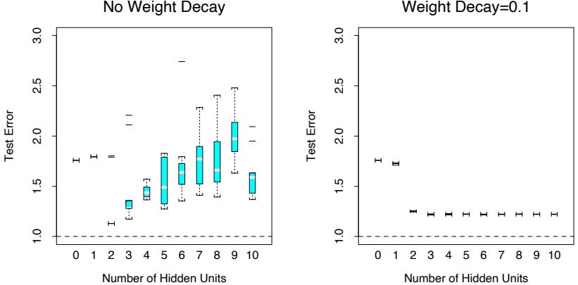
FIGURE 11.7. Boxplots of test error, for simulated data example, relative to the Bayes error. True function is a sum of two sigmoids. The test error is displayed for ten different starting weights, for a single hidden layer neural network with the number units as indicated. The two panels represent no weight decay (left) and strong weight decay λ = 0.1 (right).

FIGURE 11.8. Boxplots of test error, for simulated data example. True function is a sum of two sigmoids. The test error is displayed for ten different starting weights, for a single hidden layer neural network with ten hidden units and weight decay parameter value as indicated.

FIGURE 11.9. Examples of training cases from ZIP code data. Each image is a 16 × 16 8-bit grayscale representation of a handwritten digit.

decay parameter, and hence cross-validation of this parameter would be preferred.

11.7 Example: ZIP Code Data

This example is a character recognition task: classification of handwritten numerals. This problem captured the attention of the machine learning and neural network community for many years, and has remained a benchmark problem in the field. Figure 11.9 shows some examples of normalized handwritten digits, automatically scanned from envelopes by the U.S. Postal Service. The original scanned digits are binary and of different sizes and orientations; the images shown here have been deslanted and size normalized, resulting in 16× 16 grayscale images (Le Cun et al., 1990). These 256 pixel values are used as inputs to the neural network classifier.

A black box neural network is not ideally suited to this pattern recognition task, partly because the pixel representation of the images lack certain invariances (such as small rotations of the image). Consequently early attempts with neural networks yielded misclassification rates around 4.5% on various examples of the problem. In this section we show some of the pioneering efforts to handcraft the neural network to overcome some these deficiencies (Le Cun, 1989), which ultimately led to the state of the art in neural network performance(Le Cun et al., 1998)1.

Although current digit datasets have tens of thousands of training and test examples, the sample size here is deliberately modest in order to em-

¹The figures and tables in this example were recreated from Le Cun (1989).

FIGURE 11.10. Architecture of the five networks used in the ZIP code example.

phasize the effects. The examples were obtained by scanning some actual hand-drawn digits, and then generating additional images by random horizontal shifts. Details may be found in Le Cun (1989). There are 320 digits in the training set, and 160 in the test set.

Five different networks were fit to the data:

Net-1: No hidden layer, equivalent to multinomial logistic regression.

Net-2: One hidden layer, 12 hidden units fully connected.

Net-3: Two hidden layers locally connected.

Net-4: Two hidden layers, locally connected with weight sharing.

Net-5: Two hidden layers, locally connected, two levels of weight sharing.

These are depicted in Figure 11.10. Net-1 for example has 256 inputs, one each for the 16×16 input pixels, and ten output units for each of the digits 0–9. The predicted value ˆfk(x) represents the estimated probability that an image x has digit class k, for k = 0, 1, 2,…, 9.

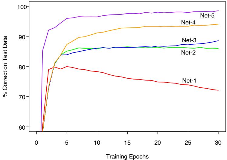
FIGURE 11.11. Test performance curves, as a function of the number of training epochs, for the five networks of Table 11.1 applied to the ZIP code data. (Le Cun, 1989)

The networks all have sigmoidal output units, and were all fit with the sum-of-squares error function. The first network has no hidden layer, and hence is nearly equivalent to a linear multinomial regression model (Exercise 11.4). Net-2 is a single hidden layer network with 12 hidden units, of the kind described above.

The training set error for all of the networks was 0%, since in all cases there are more parameters than training observations. The evolution of the test error during the training epochs is shown in Figure 11.11. The linear network (Net-1) starts to overfit fairly quickly, while test performance of the others level off at successively superior values.

The other three networks have additional features which demonstrate the power and flexibility of the neural network paradigm. They introduce constraints on the network, natural for the problem at hand, which allow for more complex connectivity but fewer parameters.

Net-3 uses local connectivity: this means that each hidden unit is connected to only a small patch of units in the layer below. In the first hidden layer (an 8×8 array), each unit takes inputs from a 3×3 patch of the input layer; for units in the first hidden layer that are one unit apart, their receptive fields overlap by one row or column, and hence are two pixels apart. In the second hidden layer, inputs are from a 5 × 5 patch, and again units that are one unit apart have receptive fields that are two units apart. The weights for all other connections are set to zero. Local connectivity makes each unit responsible for extracting local features from the layer below, and

	Network Architecture	Links	Weights	% Correct
Net-1:	Single layer network	2570	2570	80.0%
Net-2:	Two layer network	3214	3214	87.0%
Net-3:	Locally connected	1226	1226	88.5%
Net-4:	Constrained network 1	2266	1132	94.0%
Net-5:	Constrained network 2	5194	1060	98.4%

TABLE 11.1. Test set performance of five different neural networks on a handwritten digit classification example (Le Cun, 1989).

reduces considerably the total number of weights. With many more hidden units than Net-2, Net-3 has fewer links and hence weights (1226 vs. 3214), and achieves similar performance.

Net-4 and Net-5 have local connectivity with shared weights. All units in a local feature map perform the same operation on different parts of the image, achieved by sharing the same weights. The first hidden layer of Net-4 has two 8×8 arrays, and each unit takes input from a 3×3 patch just like in Net-3. However, each of the units in a single 8×8 feature map share the same set of nine weights (but have their own bias parameter). This forces the extracted features in different parts of the image to be computed by the same linear functional, and consequently these networks are sometimes known as convolutional networks. The second hidden layer of Net-4 has no weight sharing, and is the same as in Net-3. The gradient of the error function R with respect to a shared weight is the sum of the gradients of R with respect to each connection controlled by the weights in question.

Table 11.1 gives the number of links, the number of weights and the optimal test performance for each of the networks. We see that Net-4 has more links but fewer weights than Net-3, and superior test performance. Net-5 has four 4 × 4 feature maps in the second hidden layer, each unit connected to a 5 × 5 local patch in the layer below. Weights are shared in each of these feature maps. We see that Net-5 does the best, having errors of only 1.6%, compared to 13% for the “vanilla” network Net-2. The clever design of network Net-5, motivated by the fact that features of handwriting style should appear in more than one part of a digit, was the result of many person years of experimentation. This and similar networks gave better performance on ZIP code problems than any other learning method at that time (early 1990s). This example also shows that neural networks are not a fully automatic tool, as they are sometimes advertised. As with all statistical models, subject matter knowledge can and should be used to improve their performance.

This network was later outperformed by the tangent distance approach (Simard et al., 1993) described in Section 13.3.3, which explicitly incorporates natural affine invariances. At this point the digit recognition datasets become test beds for every new learning procedure, and researchers worked

408 Neural Networks

hard to drive down the error rates. As of this writing, the best error rates on a large database (60, 000 training, 10, 000 test observations), derived from standard NIST² databases, were reported to be the following: (Le Cun et al., 1998):

• 1.1% for tangent distance with a 1-nearest neighbor classifier (Section 13.3.3);
• 0.8% for a degree-9 polynomial SVM (Section 12.3);
• 0.8% for LeNet-5, a more complex version of the convolutional network described here;
• 0.7% for boosted LeNet-4. Boosting is described in Chapter 8. LeNet-4 is a predecessor of LeNet-5.

Le Cun et al. (1998) report a much larger table of performance results, and it is evident that many groups have been working very hard to bring these test error rates down. They report a standard error of 0.1% on the error estimates, which is based on a binomial average with N = 10, 000 and p ≈ 0.01. This implies that error rates within 0.1—0.2% of one another are statistically equivalent. Realistically the standard error is even higher, since the test data has been implicitly used in the tuning of the various procedures.

11.8 Discussion

Both projection pursuit regression and neural networks take nonlinear functions of linear combinations (“derived features”) of the inputs. This is a powerful and very general approach for regression and classification, and has been shown to compete well with the best learning methods on many problems.

These tools are especially effective in problems with a high signal-to-noise ratio and settings where prediction without interpretation is the goal. They are less effective for problems where the goal is to describe the physical process that generated the data and the roles of individual inputs. Each input enters into the model in many places, in a nonlinear fashion. Some authors (Hinton, 1989) plot a diagram of the estimated weights into each hidden unit, to try to understand the feature that each unit is extracting. This is limited however by the lack of identifiability of the parameter vectors αm, m = 1,…,M. Often there are solutions with α^m spanning the same linear space as the ones found during training, giving predicted values that

²The National Institute of Standards and Technology maintain large databases, including handwritten character databases; http://www.nist.gov/srd/.

are roughly the same. Some authors suggest carrying out a principal component analysis of these weights, to try to find an interpretable solution. In general, the difficulty of interpreting these models has limited their use in fields like medicine, where interpretation of the model is very important.

There has been a great deal of research on the training of neural networks. Unlike methods like CART and MARS, neural networks are smooth functions of real-valued parameters. This facilitates the development of Bayesian inference for these models. The next sections discusses a successful Bayesian implementation of neural networks.

11.9 Bayesian Neural Nets and the NIPS 2003 Challenge

A classification competition was held in 2003, in which five labeled training datasets were provided to participants. It was organized for a Neural Information Processing Systems (NIPS) workshop. Each of the data sets constituted a two-class classification problems, with different sizes and from a variety of domains (see Table 11.2). Feature measurements for a validation dataset were also available.

Participants developed and applied statistical learning procedures to make predictions on the datasets, and could submit predictions to a website on the validation set for a period of 12 weeks. With this feedback, participants were then asked to submit predictions for a separate test set and they received their results. Finally, the class labels for the validation set were released and participants had one week to train their algorithms on the combined training and validation sets, and submit their final predictions to the competition website. A total of 75 groups participated, with 20 and 16 eventually making submissions on the validation and test sets, respectively.

There was an emphasis on feature extraction in the competition. Artificial “probes” were added to the data: these are noise features with distributions resembling the real features but independent of the class labels. The percentage of probes that were added to each dataset, relative to the total set of features, is shown on Table 11.2. Thus each learning algorithm had to figure out a way of identifying the probes and downweighting or eliminating them.

A number of metrics were used to evaluate the entries, including the percentage correct on the test set, the area under the ROC curve, and a combined score that compared each pair of classifiers head-to-head. The results of the competition are very interesting and are detailed in Guyon et al. (2006). The most notable result: the entries of Neal and Zhang (2006) were the clear overall winners. In the final competition they finished first

410 Neural Networks

TABLE 11.2. NIPS 2003 challenge data sets. The column labeled p is the number of features. For the Dorothea dataset the features are binary. Ntr, Nval and Nte are the number of training, validation and test cases, respectively

Dataset	Domain	Feature Type	p	Percent Probes	Ntr	Nval	Nte
Arcene	Mass spectrometry	Dense	10,000	30	100	100	700
Dexter	Text classification	Sparse	20,000	50	300	300	2000
Dorothea	Drug discovery	Sparse	100,000	50	800	350	800
Gisette	Digit recognition	Dense	5000	30	6000	1000	6500
Madelon	Artificial	Dense	500	96	2000	600	1800

in three of the five datasets, and were 5th and 7th on the remaining two datasets.

In their winning entries, Neal and Zhang (2006) used a series of preprocessing feature-selection steps, followed by Bayesian neural networks, Dirichlet diffusion trees, and combinations of these methods. Here we focus only on the Bayesian neural network approach, and try to discern which aspects of their approach were important for its success. We rerun their programs and compare the results to boosted neural networks and boosted trees, and other related methods.

11.9.1 Bayes, Boosting and Bagging

Let us first review briefly the Bayesian approach to inference and its application to neural networks. Given training data Xtr, ytr, we assume a sampling model with parameters θ; Neal and Zhang (2006) use a two-hiddenlayer neural network, with output nodes the class probabilities Pr(Y |X, θ) for the binary outcomes. Given a prior distribution Pr(θ), the posterior distribution for the parameters is

\[\Pr(\theta|\mathbf{X\_{tr}}, \mathbf{y\_{tr}}) = \frac{\Pr(\theta)\Pr(\mathbf{y\_{tr}}|\mathbf{X\_{tr}}, \theta)}{\int \Pr(\theta)\Pr(\mathbf{y\_{tr}}|\mathbf{X\_{tr}}, \theta)d\theta} \tag{11.19}\]

For a test case with features Xnew, the predictive distribution for the label Ynew is

\[\Pr(Y\_{\text{new}}|X\_{\text{new}}, \mathbf{X}\_{\text{tr}}, \mathbf{y}\_{\text{tr}}) = \int \Pr(Y\_{\text{new}}|X\_{\text{new}}, \theta) \Pr(\theta|\mathbf{X}\_{\text{tr}}, \mathbf{y}\_{\text{tr}}) d\theta \tag{11.20}\]

(c.f. equation 8.24). Since the integral in (11.20) is intractable, sophisticated Markov Chain Monte Carlo (MCMC) methods are used to sample from the posterior distribution Pr(Ynew|Xnew, Xtr, ytr). A few hundred values θ are generated and then a simple average of these values estimates the integral. Neal and Zhang (2006) use diffuse Gaussian priors for all of the parameters. The particular MCMC approach that was used is called hybrid Monte Carlo, and may be important for the success of the method. It includes an auxiliary momentum vector and implements Hamiltonian dynamics in which the potential function is the target density. This is done to avoid random walk behavior; the successive candidates move across the sample space in larger steps. They tend to be less correlated and hence converge to the target distribution more rapidly.

Neal and Zhang (2006) also tried different forms of pre-processing of the features:

1. univariate screening using t-tests, and

2. automatic relevance determination.

In the latter method (ARD), the weights (coefficients) for the jth feature to each of the first hidden layer units all share a common prior variance σ2 ^j , and prior mean zero. The posterior distributions for each variance σ² j are computed, and the features whose posterior variance concentrates on small values are discarded.

There are thus three main features of this approach that could be important for its success:

• 1. the feature selection and pre-processing,
• 2. the neural network model, and
• 3. the Bayesian inference for the model using MCMC.

According to Neal and Zhang (2006), feature screening in (a) is carried out purely for computational efficiency; the MCMC procedure is slow with a large number of features. There is no need to use feature selection to avoid overfitting. The posterior average (11.20) takes care of this automatically.

We would like to understand the reasons for the success of the Bayesian method. In our view, power of modern Bayesian methods does not lie in their use as a formal inference procedure; most people would not believe that the priors in a high-dimensional, complex neural network model are actually correct. Rather the Bayesian/MCMC approach gives an efficient way of sampling the relevant parts of model space, and then averaging the predictions for the high-probability models.

Bagging and boosting are non-Bayesian procedures that have some similarity to MCMC in a Bayesian model. The Bayesian approach fixes the data and perturbs the parameters, according to current estimate of the posterior distribution. Bagging perturbs the data in an i.i.d fashion and then re-estimates the model to give a new set of model parameters. At the end, a simple average of the model predictions from different bagged samples is computed. Boosting is similar to bagging, but fits a model that is additive in the models of each individual base learner, which are learned using non i.i.d. samples. We can write all of these models in the form

\[\hat{f}(\mathbf{x}\_{\text{new}}) = \sum\_{\ell=1}^{L} w\_{\ell} \mathbf{E}(Y\_{\text{new}} | \mathbf{x}\_{\text{new}}, \hat{\theta}\_{\ell}) \tag{11.21}\]

412 Neural Networks

In all cases the ˆθ^ℓ are a large collection of model parameters. For the Bayesian model the w^ℓ = 1/L, and the average estimates the posterior mean (11.21) by sampling θ^ℓ from the posterior distribution. For bagging, w^ℓ = 1/L as well, and the ˆθ^ℓ are the parameters refit to bootstrap resamples of the training data. For boosting, the weights are all equal to 1, but the ˆθ^ℓ are typically chosen in a nonrandom sequential fashion to constantly improve the fit.

11.9.2 Performance Comparisons

Based on the similarities above, we decided to compare Bayesian neural networks to boosted trees, boosted neural networks, random forests and bagged neural networks on the five datasets in Table 11.2. Bagging and boosting of neural networks are not methods that we have previously used in our work. We decided to try them here, because of the success of Bayesian neural networks in this competition, and the good performance of bagging and boosting with trees. We also felt that by bagging and boosting neural nets, we could assess both the choice of model as well as the model search strategy.

Here are the details of the learning methods that were compared:

• Bayesian neural nets. The results here are taken from Neal and Zhang (2006), using their Bayesian approach to fitting neural networks. The models had two hidden layers of 20 and 8 units. We re-ran some networks for timing purposes only.
• Boosted trees. We used the gbm package (version 1.5-7) in the R language. Tree depth and shrinkage factors varied from dataset to dataset. We consistently bagged 80% of the data at each boosting iteration (the default is 50%). Shrinkage was between 0.001 and 0.1. Tree depth was between 2 and 9.
• Boosted neural networks. Since boosting is typically most effective with “weak” learners, we boosted a single hidden layer neural network with two or four units, fit with the nnet package (version 7.2-36) in R.
• Random forests. We used the R package randomForest (version 4.5-16) with default settings for the parameters.
• Bagged neural networks. We used the same architecture as in the Bayesian neural network above (two hidden layers of 20 and 8 units), fit using both Neal’s C language package “Flexible Bayesian Modeling” (2004- 11-10 release), and Matlab neural-net toolbox (version 5.1).

FIGURE 11.12. Performance of different learning methods on five problems, using both univariate screening of features (top panel) and a reduced feature set from automatic relevance determination. The error bars at the top of each plot have width equal to one standard error of the difference between two error rates. On most of the problems several competitors are within this error bound.

This analysis was carried out by Nicholas Johnson, and full details may be found in Johnson (2008)³. The results are shown in Figure 11.12 and Table 11.3.

The figure and table show Bayesian, boosted and bagged neural networks, boosted trees, and random forests, using both the screened and reduced features sets. The error bars at the top of each plot indicate one standard error of the difference between two error rates. Bayesian neural networks again emerge as the winner, although for some datasets the differences between the test error rates is not statistically significant. Random forests performs the best among the competitors using the selected feature set, while the boosted neural networks perform best with the reduced feature set, and nearly match the Bayesian neural net.

The superiority of boosted neural networks over boosted trees suggest that the neural network model is better suited to these particular problems. Specifically, individual features might not be good predictors here

³We also thank Isabelle Guyon for help in preparing the results of this section.

414 Neural Networks

TABLE 11.3. Performance of different methods. Values are average rank of test error across the five problems (low is good), and mean computation time and standard error of the mean, in minutes.

	Screened Features ARD Reduced Features
Method	Average	Average	Average	Average
	Rank	Time	Rank	Time
Bayesian neural networks	1.5	384(138)	1.6	600(186)
Boosted trees	3.4	3.03(2.5)	4.0	34.1(32.4)
Boosted neural networks	3.8	9.4(8.6)	2.2	35.6(33.5)
Random forests	2.7	1.9(1.7)	3.2	11.2(9.3)
Bagged neural networks	3.6	3.5(1.1)	4.0	6.4(4.4)

and linear combinations of features work better. However the impressive performance of random forests is at odds with this explanation, and came as a surprise to us.

Since the reduced feature sets come from the Bayesian neural network approach, only the methods that use the screened features are legitimate, self-contained procedures. However, this does suggest that better methods for internal feature selection might help the overall performance of boosted neural networks.

The table also shows the approximate training time required for each method. Here the non-Bayesian methods show a clear advantage.

Overall, the superior performance of Bayesian neural networks here may be due to the fact that

• 1. the neural network model is well suited to these five problems, and
• 2. the MCMC approach provides an efficient way of exploring the important part of the parameter space, and then averaging the resulting models according to their quality.

The Bayesian approach works well for smoothly parametrized models like neural nets; it is not yet clear that it works as well for non-smooth models like trees.

11.10 Computational Considerations

With N observations, p predictors, M hidden units and L training epochs, a neural network fit typically requires O(N pML) operations. There are many packages available for fitting neural networks, probably many more than exist for mainstream statistical methods. Because the available software varies widely in quality, and the learning problem for neural networks is sensitive to issues such as input scaling, such software should be carefully chosen and tested.

Bibliographic Notes

Projection pursuit was proposed by Friedman and Tukey (1974), and specialized to regression by Friedman and Stuetzle (1981). Huber (1985) gives a scholarly overview, and Roosen and Hastie (1994) present a formulation using smoothing splines. The motivation for neural networks dates back to McCulloch and Pitts (1943), Widrow and Hoff (1960) (reprinted in Anderson and Rosenfeld (1988)) and Rosenblatt (1962). Hebb (1949) heavily influenced the development of learning algorithms. The resurgence of neural networks in the mid 1980s was due to Werbos (1974), Parker (1985) and Rumelhart et al. (1986), who proposed the back-propagation algorithm. Today there are many books written on the topic, for a broad range of audiences. For readers of this book, Hertz et al. (1991), Bishop (1995) and Ripley (1996) may be the most informative. Bayesian learning for neural networks is described in Neal (1996). The ZIP code example was taken from Le Cun (1989); see also Le Cun et al. (1990) and Le Cun et al. (1998).

We do not discuss theoretical topics such as approximation properties of neural networks, such as the work of Barron (1993), Girosi et al. (1995) and Jones (1992). Some of these results are summarized by Ripley (1996).

Exercises

Ex. 11.1 Establish the exact correspondence between the projection pursuit regression model (11.1) and the neural network (11.5). In particular, show that the single-layer regression network is equivalent to a PPR model with gm(ω^{T m}x) = βmσ(α0^m + sm(ω^{T m}x)), where ω^m is the mth unit vector. Establish a similar equivalence for a classification network.

Ex. 11.2 Consider a neural network for a quantitative outcome as in (11.5), using squared-error loss and identity output function gk(t) = t. Suppose that the weights α^m from the input to hidden layer are nearly zero. Show that the resulting model is nearly linear in the inputs.

Ex. 11.3 Derive the forward and backward propagation equations for the cross-entropy loss function.

Ex. 11.4 Consider a neural network for a K class outcome that uses crossentropy loss. If the network has no hidden layer, show that the model is equivalent to the multinomial logistic model described in Chapter 4.

Ex. 11.5

1. Write a program to fit a single hidden layer neural network (ten hidden units) via back-propagation and weight decay.

416 Neural Networks

2. Apply it to 100 observations from the model

\[Y = \sigma(a\_1^T X) + (a\_2^T X)^2 + 0.30 \cdot Z,\]

where σ is the sigmoid function, Z is standard normal, X^T = (X1, X2), each X^j being independent standard normal, and a¹ = (3, 3), a² = (3, −3). Generate a test sample of size 1000, and plot the training and test error curves as a function of the number of training epochs, for different values of the weight decay parameter. Discuss the overfitting behavior in each case.

3. Vary the number of hidden units in the network, from 1 up to 10, and determine the minimum number needed to perform well for this task.

Ex. 11.6 Write a program to carry out projection pursuit regression, using cubic smoothing splines with fixed degrees of freedom. Fit it to the data from the previous exercise, for various values of the smoothing parameter and number of model terms. Find the minimum number of model terms necessary for the model to perform well and compare this to the number of hidden units from the previous exercise.

Ex. 11.7 Fit a neural network to the spam data of Section 9.1.2, and compare the results to those for the additive model given in that chapter. Compare both the classification performance and interpretability of the final model.

This is page 417 Printer: Opaque this

12

Support Vector Machines and Flexible Discriminants

12.1 Introduction

In this chapter we describe generalizations of linear decision boundaries for classification. Optimal separating hyperplanes are introduced in Chapter 4 for the case when two classes are linearly separable. Here we cover extensions to the nonseparable case, where the classes overlap. These techniques are then generalized to what is known as the support vector machine, which produces nonlinear boundaries by constructing a linear boundary in a large, transformed version of the feature space. The second set of methods generalize Fisher’s linear discriminant analysis (LDA). The generalizations include flexible discriminant analysis which facilitates construction of nonlinear boundaries in a manner very similar to the support vector machines, penalized discriminant analysis for problems such as signal and image classification where the large number of features are highly correlated, and mixture discriminant analysis for irregularly shaped classes.

12.2 The Support Vector Classifier

In Chapter 4 we discussed a technique for constructing an optimal separating hyperplane between two perfectly separated classes. We review this and generalize to the nonseparable case, where the classes may not be separable by a linear boundary.

FIGURE 12.1. Support vector classifiers. The left panel shows the separable case. The decision boundary is the solid line, while broken lines bound the shaded maximal margin of width 2M = 2/∥β∥. The right panel shows the nonseparable (overlap) case. The points labeled ξ^{∗ j} are on the wrong side of their margin by an amount ξ^{∗ j} = Mξ^j ; points on the correct side have ξ^{∗ j} = 0. The margin is maximized subject to a total budget ^Pξ^{i ≤} constant. Hence ^Pξ^{∗ j} is the total distance of points on the wrong side of their margin.

Our training data consists of N pairs (x1, y1),(x2, y2),…,(x^N , y^N ), with ^{xi ∈} IR^p and ^{yi ∈} {−1, ¹}. Define a hyperplane by

\[\{x \colon f(x) = x^T \beta + \beta\_0 = 0\},\tag{12.1}\]

where β is a unit vector: ∥β∥ = 1. A classification rule induced by f(x) is

\[G(x) = \text{sign}[x^T \beta + \beta\_0].\tag{12.2}\]

The geometry of hyperplanes is reviewed in Section 4.5, where we show that f(x) in (12.1) gives the signed distance from a point x to the hyperplane f(x) = x^T β+β⁰ = 0. Since the classes are separable, we can find a function ^f(x) = ^{xT β + β0} with ^yif(xi) ^&gt; ^{0 ∀}i. Hence we are able to find the hyperplane that creates the biggest margin between the training points for class 1 and −1 (see Figure 12.1). The optimization problem

\[\begin{aligned} \max\_{\beta, \beta\_0, \|\beta\| = 1} M\\ \text{subject to } y\_i(x\_i^T \beta + \beta\_0) \ge M, \ i = 1, \ldots, N, \end{aligned} \tag{12.3}\]

captures this concept. The band in the figure is M units away from the hyperplane on either side, and hence 2M units wide. It is called the margin.

We showed that this problem can be more conveniently rephrased as

\[\begin{aligned} \min\_{\beta, \beta\_0} & \|\beta\|\\ \text{subject to } y\_i(x\_i^T \beta + \beta\_0) \ge 1, \ i = 1, \dots, N, \end{aligned} \tag{12.4}\]

where we have dropped the norm constraint on β. Note that M = 1/∥β∥. Expression (12.4) is the usual way of writing the support vector criterion for separated data. This is a convex optimization problem (quadratic criterion, linear inequality constraints), and the solution is characterized in Section 4.5.2.

Suppose now that the classes overlap in feature space. One way to deal with the overlap is to still maximize M, but allow for some points to be on the wrong side of the margin. Define the slack variables ξ = (ξ1, ξ2,…, ξ^N ). There are two natural ways to modify the constraint in (12.3):

\[y\_i(x\_i^T\beta + \beta\_0) \quad \ge \quad M - \xi\_i,\tag{12.5}\]

\[\text{or}\]

\[\|y\_i(x\_i^T\beta + \beta\_0)\| \quad \ge \quad M(1-\xi\_i),\tag{12.6}\]

∀i, ξⁱ ≥ 0, #^{N i}=1 ξⁱ ≤ constant. The two choices lead to different solutions. The first choice seems more natural, since it measures overlap in actual distance from the margin; the second choice measures the overlap in relative distance, which changes with the width of the margin M. However, the first choice results in a nonconvex optimization problem, while the second is convex; thus (12.6) leads to the “standard” support vector classifier, which we use from here on.

Here is the idea of the formulation. The value ξⁱ in the constraint yi(x^{T i} β+ β0) ≥ M(1 − ξi) is the proportional amount by which the prediction f(xi) = x^{T i} β+β⁰ is on the wrong side of its margin. Hence by bounding the sum #ξi, we bound the total proportional amount by which predictions fall on the wrong side of their margin. Misclassifications occur when ξⁱ > 1, so bounding #ξⁱ at a value K say, bounds the total number of training misclassifications at K.

As in (4.48) in Section 4.5.2, we can drop the norm constraint on β, define M = 1/∥β∥, and write (12.4) in the equivalent form

\[\min \|\beta\| \quad \text{subject to} \begin{cases} \quad y\_i(x\_i^T \beta + \beta\_0) \ge 1 - \xi\_i \,\forall i, \\\quad \xi\_i \ge 0, \,\,\sum \xi\_i \le \text{constant}. \end{cases} \tag{12.7}\]

This is the usual way the support vector classifier is defined for the nonseparable case. However we find confusing the presence of the fixed scale “1” in the constraint yi(x^{T i} β +β0) ≥ 1−ξi, and prefer to start with (12.6). The right panel of Figure 12.1 illustrates this overlapping case.

By the nature of the criterion (12.7), we see that points well inside their class boundary do not play a big role in shaping the boundary. This seems like an attractive property, and one that differentiates it from linear discriminant analysis (Section 4.3). In LDA, the decision boundary is determined by the covariance of the class distributions and the positions of the class centroids. We will see in Section 12.3.3 that logistic regression is more similar to the support vector classifier in this regard.

420 12. Flexible Discriminants

12.2.1 Computing the Support Vector Classifier

The problem (12.7) is quadratic with linear inequality constraints, hence it is a convex optimization problem. We describe a quadratic programming solution using Lagrange multipliers. Computationally it is convenient to re-express (12.7) in the equivalent form

\[\begin{aligned} \min\_{\beta, \beta\_0} &\frac{1}{2} \|\beta\|^2 + C \sum\_{i=1}^N \xi\_i \\ \text{subject to} &\quad \xi\_i \ge 0, \ y\_i(x\_i^T \beta + \beta\_0) \ge 1 - \xi\_i \,\forall i, \end{aligned} \tag{12.8}\]

where the “cost” parameter C replaces the constant in (12.7); the separable case corresponds to C = ∞.

The Lagrange (primal) function is

\[L\_P = \frac{1}{2} \|\beta\|^2 + C \sum\_{i=1}^{N} \xi\_i - \sum\_{i=1}^{N} \alpha\_i [y\_i(x\_i^T \beta + \beta\_0) - (1 - \xi\_i)] - \sum\_{i=1}^{N} \mu\_i \xi\_i,\tag{12.9}\]

which we minimize w.r.t β, β⁰ and ξi. Setting the respective derivatives to zero, we get

\[\beta\_{\pm} = \sum\_{\substack{i=1 \\ \dots}}^{N} \alpha\_i y\_i x\_i,\tag{12.10}\]

\[0 \quad = \sum\_{i=1}^{N} \alpha\_i y\_i,\tag{12.11}\]

\[ \alpha\_i \quad = \ C - \mu\_i, \ \forall i,\tag{12.12} \]

as well as the positivity constraints αi, µi, ξⁱ ≥ 0 ∀i. By substituting (12.10)–(12.12) into (12.9), we obtain the Lagrangian (Wolfe) dual objective function

\[L\_D = \sum\_{i=1}^{N} \alpha\_i - \frac{1}{2} \sum\_{i=1}^{N} \sum\_{i'=1}^{N} \alpha\_i \alpha\_{i'} y\_i y\_{i'} x\_i^T x\_{i'},\tag{12.13}\]

which gives a lower bound on the objective function (12.8) for any feasible point. We maximize ^LD subject to 0 ^{≤ αi ≤ C} and #^{N i}=1 αiyⁱ = 0. In addition to (12.10)–(12.12), the Karush–Kuhn–Tucker conditions include the constraints

\[ \alpha\_i [y\_i(x\_i^T \beta + \beta\_0) - (1 - \xi\_i)] \quad = \quad 0,\tag{12.14} \]

\[ \mu\_i \xi\_i \quad = \quad 0,\tag{12.15} \]

\[y\_i(x\_i^T\beta + \beta\_0) - (1 - \xi\_i) \quad \ge \quad 0,\tag{12.16}\]

for i = 1,…,N. Together these equations (12.10)–(12.16) uniquely characterize the solution to the primal and dual problem.

From (12.10) we see that the solution for β has the form

\[ \hat{\beta} = \sum\_{i=1}^{N} \hat{\alpha}\_i y\_i x\_i,\tag{12.17} \]

with nonzero coefficients ˆαⁱ only for those observations i for which the constraints in (12.16) are exactly met (due to (12.14)). These observations are called the support vectors, since βˆ is represented in terms of them alone. Among these support points, some will lie on the edge of the margin (ˆξⁱ = 0), and hence from (12.15) and (12.12) will be characterized by 0 < αˆⁱ < C; the remainder (ˆξⁱ > 0) have ˆαⁱ = C. From (12.14) we can see that any of these margin points (0 < αˆi, ˆξⁱ = 0) can be used to solve for β0, and we typically use an average of all the solutions for numerical stability.

Maximizing the dual (12.13) is a simpler convex quadratic programming problem than the primal (12.9), and can be solved with standard techniques (Murray et al., 1981, for example).

Given the solutions βˆ⁰ and βˆ, the decision function can be written as

\[\begin{aligned} \hat{G}(x) &= \text{sign}[\hat{f}(x)] \\ &= \text{sign}[x^T \hat{\beta} + \hat{\beta}\_0]. \end{aligned} \tag{12.18}\]

The tuning parameter of this procedure is the cost parameter C.

12.2.2 Mixture Example (Continued)

Figure 12.2 shows the support vector boundary for the mixture example of Figure 2.5 on page 21, with two overlapping classes, for two different values of the cost parameter C. The classifiers are rather similar in their performance. Points on the wrong side of the boundary are support vectors. In addition, points on the correct side of the boundary but close to it (in the margin), are also support vectors. The margin is larger for C = 0.01 than it is for C = 10, 000. Hence larger values of C focus attention more on (correctly classified) points near the decision boundary, while smaller values involve data further away. Either way, misclassified points are given weight, no matter how far away. In this example the procedure is not very sensitive to choices of C, because of the rigidity of a linear boundary.

The optimal value for C can be estimated by cross-validation, as discussed in Chapter 7. Interestingly, the leave-one-out cross-validation error can be bounded above by the proportion of support points in the data. The reason is that leaving out an observation that is not a support vector will not change the solution. Hence these observations, being classified correctly by the original boundary, will be classified correctly in the cross-validation process. However this bound tends to be too high, and not generally useful for choosing C (62% and 85%, respectively, in our examples).

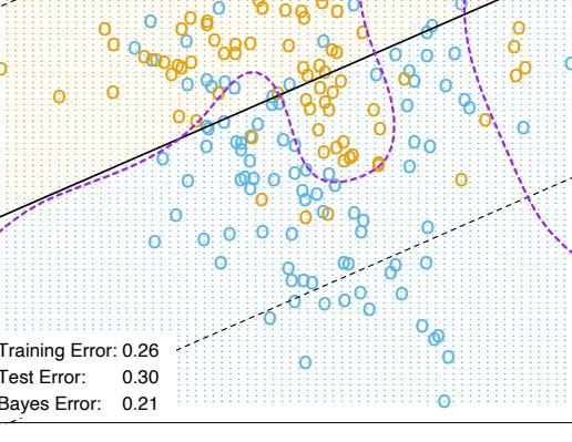
12.3 Support Vector Machines and Kernels

The support vector classifier described so far finds linear boundaries in the input feature space. As with other linear methods, we can make the procedure more flexible by enlarging the feature space using basis expansions such as polynomials or splines (Chapter 5). Generally linear boundaries in the enlarged space achieve better training-class separation, and translate to nonlinear boundaries in the original space. Once the basis functions hm(x), m = 1,…,M are selected, the procedure is the same as before. We fit the SV classifier using input features h(xi)=(h1(xi), h2(xi),…,hM(xi)), i = 1,…,N, and produce the (nonlinear) function ˆf(x) = h(x)^T βˆ + βˆ 0. The classifier is Gˆ(x) = sign( ˆf(x)) as before.

The support vector machine classifier is an extension of this idea, where the dimension of the enlarged space is allowed to get very large, infinite in some cases. It might seem that the computations would become prohibitive. It would also seem that with sufficient basis functions, the data would be separable, and overfitting would occur. We first show how the SVM technology deals with these issues. We then see that in fact the SVM classifier is solving a function-fitting problem using a particular criterion and form of regularization, and is part of a much bigger class of problems that includes the smoothing splines of Chapter 5. The reader may wish to consult Section 5.8, which provides background material and overlaps somewhat with the next two sections.

12.3.1 Computing the SVM for Classification

We can represent the optimization problem (12.9) and its solution in a special way that only involves the input features via inner products. We do this directly for the transformed feature vectors h(xi). We then see that for particular choices of h, these inner products can be computed very cheaply.

The Lagrange dual function (12.13) has the form

\[L\_D = \sum\_{i=1}^{N} \alpha\_i - \frac{1}{2} \sum\_{i=1}^{N} \sum\_{i'=1}^{N} \alpha\_i \alpha\_{i'} y\_i y\_{i'} \langle h(x\_i), h(x\_{i'}) \rangle. \tag{12.19}\]

From (12.10) we see that the solution function f(x) can be written

\[\begin{aligned} f(x) &= -h(x)^T \beta + \beta\_0 \\ &= \sum\_{i=1}^N \alpha\_i y\_i \langle h(x), h(x\_i) \rangle + \beta\_0. \end{aligned} \tag{12.20}\]

As before, given αi, β⁰ can be determined by solving yif(xi) = 1 in (12.20) for any (or all) xⁱ for which 0 < αⁱ < C.

424 12. Flexible Discriminants

So both (12.19) and (12.20) involve h(x) only through inner products. In fact, we need not specify the transformation h(x) at all, but require only knowledge of the kernel function

\[K(x, x') = \langle h(x), h(x') \rangle \tag{12.21}\]

that computes inner products in the transformed space. K should be a symmetric positive (semi-) definite function; see Section 5.8.1.

Three popular choices for K in the SVM literature are

\[\begin{aligned} d\text{th-Degree polynomial: } &K(x, x') = \left(1 + \langle x, x'\rangle\right)^d, \\ &\text{Radial basis: } &K(x, x') = \exp(-\gamma \|x - x'\|^2), \\ &\text{Neural network: } &K(x, x') = \tanh(\kappa\_1 \langle x, x'\rangle + \kappa\_2). \end{aligned} \tag{12.22}\]

Consider for example a feature space with two inputs X¹ and X2, and a polynomial kernel of degree 2. Then

\[\begin{split} K(X, X') &= (1 + \langle X, X' \rangle)^2 \\ &= (1 + X\_1 X\_1' + X\_2 X\_2')^2 \\ &= 1 + 2X\_1 X\_1' + 2X\_2 X\_2' + (X\_1 X\_1')^2 + (X\_2 X\_2')^2 + 2X\_1 X\_1' X\_2 X\_2'. \end{split} \tag{12.23}\]

Then ^M = 6, and if we choose ^h1(X) = 1, ^h2(X) = ^√ √ 2X1, h3(X) = 2X2, h4(X) = X^{2 1} , h5(X) = X^{2 2} , and ^h6(X) = ^√2X1X2, then ^K(X, X′ ) = ⟨h(X), h(X′ )⟩. From (12.20) we see that the solution can be written

\[\hat{f}(x) = \sum\_{i=1}^{N} \hat{\alpha}\_i y\_i K(x, x\_i) + \hat{\beta}\_0. \tag{12.24}\]

The role of the parameter C is clearer in an enlarged feature space, since perfect separation is often achievable there. A large value of C will discourage any positive ξi, and lead to an overfit wiggly boundary in the original feature space; a small value of C will encourage a small value of ∥β∥, which in turn causes f(x) and hence the boundary to be smoother. Figure 12.3 show two nonlinear support vector machines applied to the mixture example of Chapter 2. The regularization parameter was chosen in both cases to achieve good test error. The radial basis kernel produces a boundary quite similar to the Bayes optimal boundary for this example; compare Figure 2.5.

In the early literature on support vectors, there were claims that the kernel property of the support vector machine is unique to it and allows one to finesse the curse of dimensionality. Neither of these claims is true, and we go into both of these issues in the next three subsections.

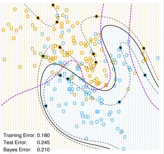
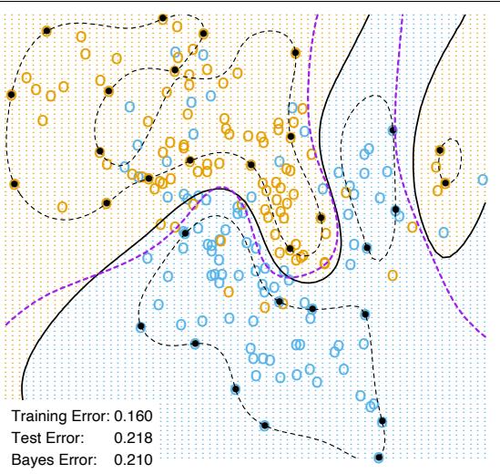
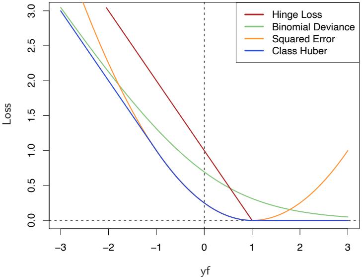
FIGURE 12.4. The support vector loss function (hinge loss), compared to the negative log-likelihood loss (binomial deviance) for logistic regression, squared-error loss, and a “Huberized” version of the squared hinge loss. All are shown as a function of yf rather than f, because of the symmetry between the y = +1 and y = −1 case. The deviance and Huber have the same asymptotes as the SVM loss, but are rounded in the interior. All are scaled to have the limiting left-tail slope of −1.

12.3.2 The SVM as a Penalization Method

With f(x) = h(x)^T β + β0, consider the optimization problem

\[\min\_{\beta\_0, \beta} \sum\_{i=1}^{N} [1 - y\_i f(x\_i)]\_+ + \frac{\lambda}{2} ||\beta||^2 \tag{12.25}\]

where the subscript “+” indicates positive part. This has the form loss + penalty, which is a familiar paradigm in function estimation. It is easy to show (Exercise 12.1) that the solution to (12.25), with λ = 1/C, is the same as that for (12.8).

Examination of the “hinge” loss function L(y, f) = [1 − yf]⁺ shows that it is reasonable for two-class classification, when compared to other more traditional loss functions. Figure 12.4 compares it to the log-likelihood loss for logistic regression, as well as squared-error loss and a variant thereof. The (negative) log-likelihood or binomial deviance has similar tails as the SVM loss, giving zero penalty to points well inside their margin, and a

TABLE 12.1. The population minimizers for the different loss functions in Figure 12.4. Logistic regression uses the binomial log-likelihood or deviance. Linear discriminant analysis (Exercise 4.2) uses squared-error loss. The SVM hinge loss estimates the mode of the posterior class probabilities, whereas the others estimate a linear transformation of these probabilities.

Loss Function	L[y, f(x)]	Minimizing Function
Binomial Deviance	log[1 + e−yf(x) ]	f(x) = log Pr(Y = +1 x) Pr(Y = -1 x)
SVM Hinge Loss	[1 − yf(x)]+	f(x) = sign[Pr(Y = +1 x) − 1 2 ]
Squared Error	[y − f(x)]2 = [1 − yf(x)]2	f(x) = 2Pr(Y = +1 x) − 1
“Huberised” Square Hinge Loss	−4yf(x), yf(x) < -1 [1 − yf(x)]2 otherwise +	f(x) = 2Pr(Y = +1 x) − 1

linear penalty to points on the wrong side and far away. Squared-error, on the other hand gives a quadratic penalty, and points well inside their own margin have a strong influence on the model as well. The squared hinge loss L(y, f) = [1 − yf] 2 ⁺ is like the quadratic, except it is zero for points inside their margin. It still rises quadratically in the left tail, and will be less robust than hinge or deviance to misclassified observations. Recently Rosset and Zhu (2007) proposed a “Huberized” version of the squared hinge loss, which converts smoothly to a linear loss at yf = −1.

We can characterize these loss functions in terms of what they are estimating at the population level. We consider minimizing EL(Y,f(X)). Table 12.1 summarizes the results. Whereas the hinge loss estimates the classifier G(x) itself, all the others estimate a transformation of the class posterior probabilities. The “Huberized” square hinge loss shares attractive properties of logistic regression (smooth loss function, estimates probabilities), as well as the SVM hinge loss (support points).

Formulation (12.25) casts the SVM as a regularized function estimation problem, where the coefficients of the linear expansion f(x) = β⁰ +h(x)^T β are shrunk toward zero (excluding the constant). If h(x) represents a hierarchical basis having some ordered structure (such as ordered in roughness),

428 12. Flexible Discriminants

then the uniform shrinkage makes more sense if the rougher elements h^j in the vector h have smaller norm.

All the loss-function in Table 12.1 except squared-error are so called “margin maximizing loss-functions” (Rosset et al., 2004b). This means that if the data are separable, then the limit of ^βˆ^λ in (12.25) as ^{λ →} 0 defines the optimal separating hyperplane1.

12.3.3 Function Estimation and Reproducing Kernels

Here we describe SVMs in terms of function estimation in reproducing kernel Hilbert spaces, where the kernel property abounds. This material is discussed in some detail in Section 5.8. This provides another view of the support vector classifier, and helps to clarify how it works.

Suppose the basis h arises from the (possibly finite) eigen-expansion of a positive definite kernel K,

\[K(x, x') = \sum\_{m=1}^{\infty} \phi\_m(x)\phi\_m(x')\delta\_m \tag{12.26}\]

and ^hm(x) = ^√δmφm(x). Then with ^{θm = √}δmβm, we can write (12.25) as

\[\min\_{\beta\_0, \theta} \sum\_{i=1}^{N} \left[ 1 - y\_i(\beta\_0 + \sum\_{m=1}^{\infty} \theta\_m \phi\_m(x\_i)) \right]\_+ + \frac{\lambda}{2} \sum\_{m=1}^{\infty} \frac{\theta\_m^2}{\delta\_m}. \tag{12.27}\]

Now (12.27) is identical in form to (5.49) on page 169 in Section 5.8, and the theory of reproducing kernel Hilbert spaces described there guarantees a finite-dimensional solution of the form

\[f(x) = \beta\_0 + \sum\_{i=1}^{N} \alpha\_i K(x, x\_i). \tag{12.28}\]

In particular we see there an equivalent version of the optimization criterion (12.19) [Equation (5.67) in Section 5.8.2; see also Wahba et al. (2000)],

\[\min\_{\beta\_0, \alpha} \sum\_{i=1}^N (1 - y\_i f(x\_i))\_+ + \frac{\lambda}{2} \alpha^T \mathbf{K} \alpha,\tag{12.29}\]

where K is the N × N matrix of kernel evaluations for all pairs of training features (Exercise 12.2).

These models are quite general, and include, for example, the entire family of smoothing splines, additive and interaction spline models discussed

¹For logistic regression with separable data, βˆ^λ diverges, but βˆλ/||βˆ^λ converges to the optimal separating direction.

in Chapters 5 and 9, and in more detail in Wahba (1990) and Hastie and Tibshirani (1990). They can be expressed more generally as

\[\min\_{f \in \mathcal{H}} \sum\_{i=1}^{N} [1 - y\_i f(x\_i)]\_+ + \lambda J(f), \tag{12.30}\]

where H is the structured space of functions, and J(f) an appropriate regularizer on that space. For example, suppose H is the space of additive functions f(x) = #^{p j}=1 ^fj (x^j ), and ^J(f) = # j 5 {f′′ ^j (x^j )}2dx^j . Then the solution to (12.30) is an additive cubic spline, and has a kernel representation (12.28) with K(x, x′ ) = #^{p j}=1 K^j (x^j , x′ ^j ). Each of the K^j is the kernel appropriate for the univariate smoothing spline in x^j (Wahba, 1990).

Conversely this discussion also shows that, for example, any of the kernels described in (12.22) above can be used with any convex loss function, and will also lead to a finite-dimensional representation of the form (12.28). Figure 12.5 uses the same kernel functions as in Figure 12.3, except using the binomial log-likelihood as a loss function². The fitted function is hence an estimate of the log-odds,

\[\begin{aligned} \hat{f}(x) &= \quad \log \frac{\hat{\Pr}(Y=+1|x)}{\hat{\Pr}(Y=-1|x)}\\ &= \quad \hat{\beta}\_0 + \sum\_{i=1}^N \hat{\alpha}\_i K(x, x\_i), \end{aligned} \tag{12.31}\]

or conversely we get an estimate of the class probabilities

\[\hat{\Pr}(Y=+1|x) = \frac{1}{1 + e^{-\hat{\beta}\_0 - \sum\_{i=1}^{N} \hat{\alpha}\_i K(x, x\_i)}}. \tag{12.32}\]

The fitted models are quite similar in shape and performance. Examples and more details are given in Section 5.8.

It does happen that for SVMs, a sizable fraction of the N values of αⁱ can be zero (the nonsupport points). In the two examples in Figure 12.3, these fractions are 42% and 45%, respectively. This is a consequence of the piecewise linear nature of the first part of the criterion (12.25). The lower the class overlap (on the training data), the greater this fraction will be. Reducing λ will generally reduce the overlap (allowing a more flexible f). A small number of support points means that ˆf(x) can be evaluated more quickly, which is important at lookup time. Of course, reducing the overlap too much can lead to poor generalization.

²Ji Zhu assisted in the preparation of these examples.

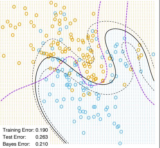
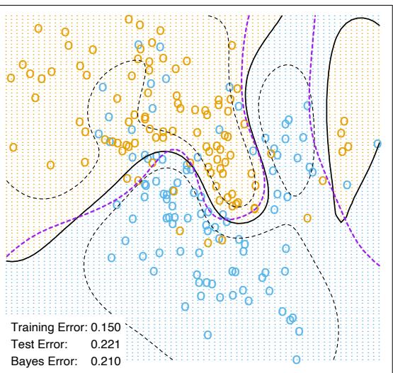
		Test Error (SE)
	Method	No Noise Features	Six Noise Features
1	SV Classifier	0.450 (0.003)	0.472 (0.003)
2	SVM/poly 2	0.078 (0.003)	0.152 (0.004)
3	SVM/poly 5	0.180 (0.004)	0.370 (0.004)
4	SVM/poly 10	0.230 (0.003)	0.434 (0.002)
5	BRUTO	0.084 (0.003)	0.090 (0.003)
6	MARS	0.156 (0.004)	0.173 (0.005)
	Bayes	0.029	0.029

TABLE 12.2. Skin of the orange: Shown are mean (standard error of the mean) of the test error over 50 simulations. BRUTO fits an additive spline model adaptively, while MARS fits a low-order interaction model adaptively.

12.3.4 SVMs and the Curse of Dimensionality

In this section, we address the question of whether SVMs have some edge on the curse of dimensionality. Notice that in expression (12.23) we are not allowed a fully general inner product in the space of powers and products. For example, all terms of the form 2XjX′ ^j are given equal weight, and the kernel cannot adapt itself to concentrate on subspaces. If the number of features p were large, but the class separation occurred only in the linear subspace spanned by say X¹ and X2, this kernel would not easily find the structure and would suffer from having many dimensions to search over. One would have to build knowledge about the subspace into the kernel; that is, tell it to ignore all but the first two inputs. If such knowledge were available a priori, much of statistical learning would be made much easier. A major goal of adaptive methods is to discover such structure.

We support these statements with an illustrative example. We generated 100 observations in each of two classes. The first class has four standard normal independent features X1, X2, X3, X4. The second class also has four standard normal independent features, but conditioned on 9 ^≤ #X^{2 j} ≤ 16. This is a relatively easy problem. As a second harder problem, we augmented the features with an additional six standard Gaussian noise features. Hence the second class almost completely surrounds the first, like the skin surrounding the orange, in a four-dimensional subspace. The Bayes error rate for this problem is 0.029 (irrespective of dimension). We generated 1000 test observations to compare different procedures. The average test errors over 50 simulations, with and without noise features, are shown in Table 12.2.

Line 1 uses the support vector classifier in the original feature space. Lines 2–4 refer to the support vector machine with a 2-, 5- and 10-dimensional polynomial kernel. For all support vector procedures, we chose the cost parameter C to minimize the test error, to be as fair as possible to the

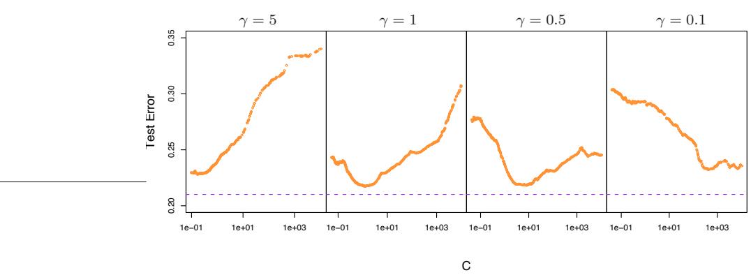
Test Error Curves − SVM with Radial Kernel

FIGURE 12.6. Test-error curves as a function of the cost parameter C for the radial-kernel SVM classifier on the mixture data. At the top of each plot is the scale parameter ^γ for the radial kernel: ^Kγ(x, y) = exp ⁻γ||^{x − y}||². The optimal value for C depends quite strongly on the scale of the kernel. The Bayes error rate is indicated by the broken horizontal lines.

method. Line 5 fits an additive spline model to the (−1, +1) response by least squares, using the BRUTO algorithm for additive models, described in Hastie and Tibshirani (1990). Line 6 uses MARS (multivariate adaptive regression splines) allowing interaction of all orders, as described in Chapter 9; as such it is comparable with the SVM/poly 10. Both BRUTO and MARS have the ability to ignore redundant variables. Test error was not used to choose the smoothing parameters in either of lines 5 or 6.

In the original feature space, a hyperplane cannot separate the classes, and the support vector classifier (line 1) does poorly. The polynomial support vector machine makes a substantial improvement in test error rate, but is adversely affected by the six noise features. It is also very sensitive to the choice of kernel: the second degree polynomial kernel (line 2) does best, since the true decision boundary is a second-degree polynomial. However, higher-degree polynomial kernels (lines 3 and 4) do much worse. BRUTO performs well, since the boundary is additive. BRUTO and MARS adapt well: their performance does not deteriorate much in the presence of noise.

12.3.5 A Path Algorithm for the SVM Classifier

The regularization parameter for the SVM classifier is the cost parameter C, or its inverse λ in (12.25). Common usage is to set C high, leading often to somewhat overfit classifiers.

Figure 12.6 shows the test error on the mixture data as a function of C, using different radial-kernel parameters γ. When γ = 5 (narrow peaked kernels), the heaviest regularization (small C) is called for. With γ = 1

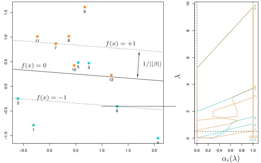
FIGURE 12.7. A simple example illustrates the SVM path algorithm. (left panel:) This plot illustrates the state of the model at λ = 0.05. The ’’+1” points are orange, the “−1” blue. λ = 1/2, and the width of the soft margin is 2/||β|| = 2 × 0.587. Two blue points {3, 5} are misclassified, while the two orange points {10, 12} are correctly classified, but on the wrong side of their margin f(x) = +1; each of these has yif(xi) < 1. The three square shaped points {2, 6, 7} are exactly on their margins. (right panel:) This plot shows the piecewise linear profiles αi(λ). The horizontal broken line at λ = 1/2 indicates the state of the αⁱ for the model in the left plot.

(the value used in Figure 12.3), an intermediate value of C is required. Clearly in situations such as these, we need to determine a good choice for C, perhaps by cross-validation. Here we describe a path algorithm (in the spirit of Section 3.8) for efficiently fitting the entire sequence of SVM models obtained by varying C.

It is convenient to use the loss+penalty formulation (12.25), along with Figure 12.4. This leads to a solution for β at a given value of λ:

\[ \beta\_{\lambda} = \frac{1}{\lambda} \sum\_{i=1}^{N} \alpha\_i y\_i x\_i. \tag{12.33} \]

The αⁱ are again Lagrange multipliers, but in this case they all lie in [0, 1].

Figure 12.7 illustrates the setup. It can be shown that the KKT optimality conditions imply that the labeled points (xi, yi) fall into three distinct groups:

434 12. Flexible Discriminants

• Observations correctly classified and outside their margins. They have yif(xi) > 1, and Lagrange multipliers αⁱ = 0. Examples are the orange points 8, 9 and 11, and the blue points 1 and 4.
• Observations sitting on their margins with yif(xi) = 1, with Lagrange multipliers αⁱ ∈ [0, 1]. Examples are the orange 7 and the blue 2 and 8.
• Observations inside their margins have yif(xi) < 1, with αⁱ = 1. Examples are the blue 3 and 5, and the orange 10 and 12.

The idea for the path algorithm is as follows. Initially λ is large, the margin 1/||βλ|| is wide, and all points are inside their margin and have αⁱ = 1. As λ decreases, 1/||βλ|| decreases, and the margin gets narrower. Some points will move from inside their margins to outside their margins, and their αⁱ will change from 1 to 0. By continuity of the αi(λ), these points will linger on the margin during this transition. From (12.33) we see that the points with αⁱ = 1 make fixed contributions to β(λ), and those with αⁱ = 0 make no contribution. So all that changes as λ decreases are the αⁱ ∈ [0, 1] of those (small number) of points on the margin. Since all these points have yif(xi) = 1, this results in a small set of linear equations that prescribe how αi(λ) and hence β^λ changes during these transitions. This results in piecewise linear paths for each of the αi(λ). The breaks occur when points cross the margin. Figure 12.7 (right panel) shows the αi(λ) profiles for the small example in the left panel.

Although we have described this for linear SVMs, exactly the same idea works for nonlinear models, in which (12.33) is replaced by

\[f\_{\lambda}(x) = \frac{1}{\lambda} \sum\_{i=1}^{N} \alpha\_i y\_i K(x, x\_i). \tag{12.34}\]

Details can be found in Hastie et al. (2004). An R package svmpath is available on CRAN for fitting these models.

12.3.6 Support Vector Machines for Regression

In this section we show how SVMs can be adapted for regression with a quantitative response, in ways that inherit some of the properties of the SVM classifier. We first discuss the linear regression model

\[f(x) = x^T \beta + \beta\_0,\tag{12.35}\]

and then handle nonlinear generalizations. To estimate β, we consider minimization of

\[H(\beta, \beta\_0) = \sum\_{i=1}^{N} V(y\_i - f(x\_i)) + \frac{\lambda}{2} ||\beta||^2,\tag{12.36}\]

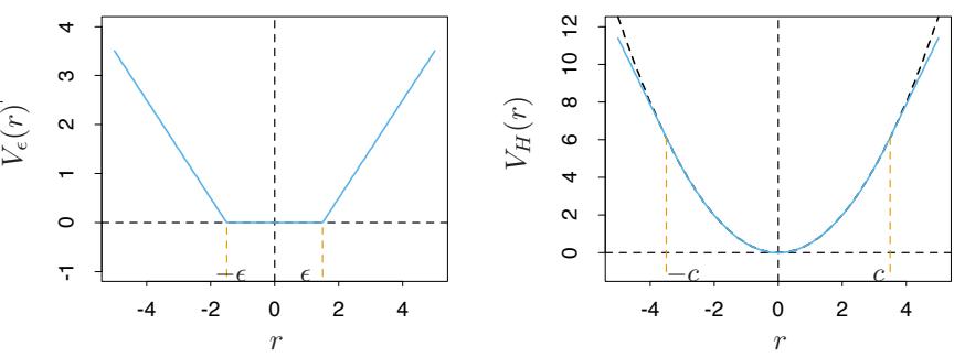
FIGURE 12.8. The left panel shows the ϵ-insensitive error function used by the support vector regression machine. The right panel shows the error function used in Huber’s robust regression (blue curve). Beyond |c|, the function changes from quadratic to linear.

where

\[V\_{\epsilon}(r) = \begin{cases} 0 & \text{if } |r| < \epsilon, \\ |r| - \epsilon, & \text{otherwise.} \end{cases} \tag{12.37}\]

This is an “ϵ-insensitive” error measure, ignoring errors of size less than ϵ (left panel of Figure 12.8). There is a rough analogy with the support vector classification setup, where points on the correct side of the decision boundary and far away from it, are ignored in the optimization. In regression, these “low error” points are the ones with small residuals.

It is interesting to contrast this with error measures used in robust regression in statistics. The most popular, due to Huber (1964), has the form

\[V\_H(r) = \begin{cases} r^2/2 & \text{if } |r| \le c, \\ c|r| - c^2/2, \quad |r| > c, \end{cases} \tag{12.38}\]

shown in the right panel of Figure 12.8. This function reduces from quadratic to linear the contributions of observations with absolute residual greater than a prechosen constant c. This makes the fitting less sensitive to outliers. The support vector error measure (12.37) also has linear tails (beyond ϵ), but in addition it flattens the contributions of those cases with small residuals.

If βˆ, βˆ⁰ are the minimizers of H, the solution function can be shown to have the form

\[\hat{\beta}^{\quad} \quad = \sum\_{i=1}^{N} (\hat{\alpha}\_i^\* - \hat{\alpha}\_i) x\_i,\tag{12.39}\]

\[\hat{f}(x) \quad = \sum\_{i=1}^{N} (\hat{\alpha}\_i^\* - \hat{\alpha}\_i) \langle x, x\_i \rangle + \beta\_0,\tag{12.40}\]

436 12. Flexible Discriminants

where ˆαi, αˆ^{∗ i} are positive and solve the quadratic programming problem

\[\min\_{\alpha\_{i},\alpha\_{i}^{\*}} \epsilon \sum\_{i=1}^{N} (\alpha\_{i}^{\*} + \alpha\_{i}) - \sum\_{i=1}^{N} y\_{i} (\alpha\_{i}^{\*} - \alpha\_{i}) + \frac{1}{2} \sum\_{i,i'=1}^{N} (\alpha\_{i}^{\*} - \alpha\_{i})(\alpha\_{i'}^{\*} - \alpha\_{i'}) \langle x\_{i}, x\_{i'} \rangle\]

subject to the constraints

\[\begin{aligned} 0 \le \alpha\_i, &\alpha\_i^\* \le 1/\lambda, \\ \sum\_{i=1}^N (\alpha\_i^\* - \alpha\_i) &= 0, \\ \alpha\_i \alpha\_i^\* &= 0. \end{aligned} \tag{12.41}\]

Due to the nature of these constraints, typically only a subset of the solution values (ˆα^{∗ i} − αˆi) are nonzero, and the associated data values are called the support vectors. As was the case in the classification setting, the solution depends on the input values only through the inner products ⟨xi, xi′ ⟩. Thus we can generalize the methods to richer spaces by defining an appropriate inner product, for example, one of those defined in (12.22).

Note that there are parameters, ϵ and λ, associated with the criterion (12.36). These seem to play different roles. ϵ is a parameter of the loss function Vϵ, just like c is for VH. Note that both V^ϵ and V^H depend on the scale of y and hence r. If we scale our response (and hence use VH(r/σ) and Vϵ(r/σ) instead), then we might consider using preset values for c and ϵ (the value c = 1.345 achieves 95% efficiency for the Gaussian). The quantity λ is a more traditional regularization parameter, and can be estimated for example by cross-validation.

12.3.7 Regression and Kernels

As discussed in Section 12.3.3, this kernel property is not unique to support vector machines. Suppose we consider approximation of the regression function in terms of a set of basis functions {hm(x)}, m = 1, 2,…,M:

\[f(x) = \sum\_{m=1}^{M} \beta\_m h\_m(x) + \beta\_0. \tag{12.42}\]

To estimate β and β⁰ we minimize

\[H(\beta, \beta\_0) = \sum\_{i=1}^{N} V(y\_i - f(x\_i)) + \frac{\lambda}{2} \sum \beta\_m^2 \tag{12.43}\]

for some general error measure V (r). For any choice of V (r), the solution ˆf(x) = #βˆmhm(x) + βˆ⁰ has the form

\[\hat{f}(x) = \sum\_{i=1}^{N} \hat{a}\_i K(x, x\_i) \tag{12.44}\]

with K(x, y) = #^{M m}=1 hm(x)hm(y). Notice that this has the same form as both the radial basis function expansion and a regularization estimate, discussed in Chapters 5 and 6.

For concreteness, let’s work out the case ^V (r) = ^r2. Let ^H be the ^{N ×M} basis matrix with imth element hm(xi), and suppose that M>N is large. For simplicity we assume that β⁰ = 0, or that the constant is absorbed in h; see Exercise 12.3 for an alternative.

We estimate β by minimizing the penalized least squares criterion

\[H(\beta) = \left(\mathbf{y} - \mathbf{H}\beta\right)^T \left(\mathbf{y} - \mathbf{H}\beta\right) + \lambda \left\|\beta\right\|^2. \tag{12.45}\]

The solution is

\[ \hat{\mathbf{y}} = \mathbf{H}\hat{\boldsymbol{\beta}}\tag{12.46} \]

with βˆ determined by

\[-\mathbf{H}^T(\mathbf{y} - \mathbf{H}\hat{\boldsymbol{\beta}}) + \lambda\hat{\boldsymbol{\beta}} = 0.\tag{12.47}\]

From this it appears that we need to evaluate the M × M matrix of inner products in the transformed space. However, we can premultiply by H to give

\[\mathbf{H}\hat{\boldsymbol{\beta}} = (\mathbf{H}\mathbf{H}^T + \lambda\mathbf{I})^{-1}\mathbf{H}\mathbf{H}^T\mathbf{y}.\tag{12.48}\]

The ^{N × N} matrix HH^T consists of inner products between pairs of observations i, i′ ; that is, the evaluation of an inner product kernel {HH^T }i,i′ ⁼ K(xi, xi′ ). It is easy to show (12.44) directly in this case, that the predicted values at an arbitrary x satisfy

\[\begin{aligned} \hat{f}(x) &= \quad h(x)^T \hat{\beta} \\ &= \quad \sum\_{i=1}^N \hat{\alpha}\_i K(x, x\_i), \end{aligned} \tag{12.49}\]

where ˆα = (HH^T +λI)⁻1y. As in the support vector machine, we need not specify or evaluate the large set of functions h1(x), h2(x),…,hM(x). Only the inner product kernel K(xi, xi′ ) need be evaluated, at the N training points for each i, i′ and at points x for predictions there. Careful choice of h^m (such as the eigenfunctions of particular, easy-to-evaluate kernels K) means, for example, that HH^T can be computed at a cost of N2/2 evaluations of K, rather than the direct cost N2M.

Note, however, that this property depends on the choice of squared norm ^∥β∥² in the penalty. It does not hold, for example, for the ^L1 norm ^|β|, which may lead to a superior model.

438 12. Flexible Discriminants

12.3.8 Discussion

The support vector machine can be extended to multiclass problems, essentially by solving many two-class problems. A classifier is built for each pair of classes, and the final classifier is the one that dominates the most (Kressel, 1999; Friedman, 1996; Hastie and Tibshirani, 1998). Alternatively, one could use the multinomial loss function along with a suitable kernel, as in Section 12.3.3. SVMs have applications in many other supervised and unsupervised learning problems. At the time of this writing, empirical evidence suggests that it performs well in many real learning problems.

Finally, we mention the connection of the support vector machine and structural risk minimization (7.9). Suppose the training points (or their basis expansion) are contained in a sphere of radius R, and let G(x) = sign[f(x)] = sign[β^T x + β0] as in (12.2). Then one can show that the class of functions {G(x), ∥β∥ ≤ A} has VC-dimension h satisfying

\[h \le R^2 A^2. \tag{12.50}\]

If f(x) separates the training data, optimally for ∥β∥ ≤ A, then with probability at least 1 − η over training sets (Vapnik, 1996, page 139):

\[\text{Error}\_{\text{Test}} \le 4 \frac{h[\log\left(2N/h\right) + 1] - \log\left(\eta/4\right)}{N}.\tag{12.51}\]

The support vector classifier was one of the first practical learning procedures for which useful bounds on the VC dimension could be obtained, and hence the SRM program could be carried out. However in the derivation, balls are put around the data points—a process that depends on the observed values of the features. Hence in a strict sense, the VC complexity of the class is not fixed a priori, before seeing the features.

The regularization parameter C controls an upper bound on the VC dimension of the classifier. Following the SRM paradigm, we could choose C by minimizing the upper bound on the test error, given in (12.51). However, it is not clear that this has any advantage over the use of cross-validation for choice of C.

12.4 Generalizing Linear Discriminant Analysis

In Section 4.3 we discussed linear discriminant analysis (LDA), a fundamental tool for classification. For the remainder of this chapter we discuss a class of techniques that produce better classifiers than LDA by directly generalizing LDA.

Some of the virtues of LDA are as follows:

• It is a simple prototype classifier. A new observation is classified to the class with closest centroid. A slight twist is that distance is measured in the Mahalanobis metric, using a pooled covariance estimate.

• LDA is the estimated Bayes classifier if the observations are multivariate Gaussian in each class, with a common covariance matrix. Since this assumption is unlikely to be true, this might not seem to be much of a virtue.
• The decision boundaries created by LDA are linear, leading to decision rules that are simple to describe and implement.
• LDA provides natural low-dimensional views of the data. For example, Figure 12.12 is an informative two-dimensional view of data in 256 dimensions with ten classes.
• Often LDA produces the best classification results, because of its simplicity and low variance. LDA was among the top three classifiers for 11 of the 22 datasets studied in the STATLOG project (Michie et al., 1994)³.

Unfortunately the simplicity of LDA causes it to fail in a number of situations as well:

• Often linear decision boundaries do not adequately separate the classes. When N is large, it is possible to estimate more complex decision boundaries. Quadratic discriminant analysis (QDA) is often useful here, and allows for quadratic decision boundaries. More generally we would like to be able to model irregular decision boundaries.
• The aforementioned shortcoming of LDA can often be paraphrased by saying that a single prototype per class is insufficient. LDA uses a single prototype (class centroid) plus a common covariance matrix to describe the spread of the data in each class. In many situations, several prototypes are more appropriate.
• At the other end of the spectrum, we may have way too many (correlated) predictors, for example, in the case of digitized analogue signals and images. In this case LDA uses too many parameters, which are estimated with high variance, and its performance suffers. In cases such as this we need to restrict or regularize LDA even further.

In the remainder of this chapter we describe a class of techniques that attend to all these issues by generalizing the LDA model. This is achieved largely by three different ideas.

The first idea is to recast the LDA problem as a linear regression problem. Many techniques exist for generalizing linear regression to more flexible, nonparametric forms of regression. This in turn leads to more flexible forms of discriminant analysis, which we call FDA. In most cases of interest, the

³This study predated the emergence of SVMs.

440 12. Flexible Discriminants

regression procedures can be seen to identify an enlarged set of predictors via basis expansions. FDA amounts to LDA in this enlarged space, the same paradigm used in SVMs.

In the case of too many predictors, such as the pixels of a digitized image, we do not want to expand the set: it is already too large. The second idea is to fit an LDA model, but penalize its coefficients to be smooth or otherwise coherent in the spatial domain, that is, as an image. We call this procedure penalized discriminant analysis or PDA. With FDA itself, the expanded basis set is often so large that regularization is also required (again as in SVMs). Both of these can be achieved via a suitably regularized regression in the context of the FDA model.

The third idea is to model each class by a mixture of two or more Gaussians with different centroids, but with every component Gaussian, both within and between classes, sharing the same covariance matrix. This allows for more complex decision boundaries, and allows for subspace reduction as in LDA. We call this extension mixture discriminant analysis or MDA.

All three of these generalizations use a common framework by exploiting their connection with LDA.

12.5 Flexible Discriminant Analysis

In this section we describe a method for performing LDA using linear regression on derived responses. This in turn leads to nonparametric and flexible alternatives to LDA. As in Chapter 4, we assume we have observations with a quantitative response G falling into one of K classes G = {1,…,K}, each having measured features ^X. Suppose ^θ : ^G 5→ IR¹ is a function that assigns scores to the classes, such that the transformed class labels are optimally predicted by linear regression on X: If our training sample has the form (gi, xi), i = 1, 2,…,N, then we solve

\[\min\_{\beta, \theta} \sum\_{i=1}^{N} \left( \theta(g\_i) - x\_i^T \beta \right)^2,\tag{12.52}\]

with restrictions on θ to avoid a trivial solution (mean zero and unit variance over the training data). This produces a one-dimensional separation between the classes.

More generally, we can find up to L ≤ K −1 sets of independent scorings for the class labels, θ1, θ2,…, θL, and L corresponding linear maps ηℓ(X) = X^T βℓ, ℓ = 1,…,L, chosen to be optimal for multiple regression in IRp. The scores θℓ(g) and the maps β^ℓ are chosen to minimize the average squared residual,

\[ASR = \frac{1}{N} \sum\_{\ell=1}^{L} \left[ \sum\_{i=1}^{N} \left( \theta\_{\ell}(g\_i) - x\_i^T \beta\_{\ell} \right)^2 \right]. \tag{12.53}\]

The set of scores are assumed to be mutually orthogonal and normalized with respect to an appropriate inner product to prevent trivial zero solutions.

Why are we going down this road? It can be shown that the sequence of discriminant (canonical) vectors ν^ℓ derived in Section 4.3.3 are identical to the sequence β^ℓ up to a constant (Mardia et al., 1979; Hastie et al., 1995). Moreover, the Mahalanobis distance of a test point x to the kth class centroid ˆµ^k is given by

\[\delta\_J(x,\hat{\mu}\_k) = \sum\_{\ell=1}^{K-1} w\_\ell (\hat{\eta}\_\ell(x) - \bar{\eta}\_\ell^k)^2 + D(x),\tag{12.54}\]

where ¯η^{k ℓ} is the mean of the ˆηℓ(xi) in the kth class, and D(x) does not depend on k. Here w^ℓ are coordinate weights that are defined in terms of the mean squared residual r^{2 ℓ} of the ℓth optimally scored fit

\[w\_{\ell} = \frac{1}{r\_{\ell}^2 (1 - r\_{\ell}^2)}.\tag{12.55}\]

In Section 4.3.2 we saw that these canonical distances are all that is needed for classification in the Gaussian setup, with equal covariances in each class. To summarize:

LDA can be performed by a sequence of linear regressions, followed by classification to the closest class centroid in the space of fits. The analogy applies both to the reduced rank version, or the full rank case when L = K − 1.

The real power of this result is in the generalizations that it invites. We can replace the linear regression fits ηℓ(x) = x^T β^ℓ by far more flexible, nonparametric fits, and by analogy achieve a more flexible classifier than LDA. We have in mind generalized additive fits, spline functions, MARS models and the like. In this more general form the regression problems are defined via the criterion

\[ASR(\{\theta\_\ell, \eta\_\ell\}\_{\ell=1}^L) = \frac{1}{N} \sum\_{\ell=1}^L \left[ \sum\_{i=1}^N \left( \theta\_\ell(g\_i) - \eta\_\ell(x\_i) \right)^2 + \lambda J(\eta\_\ell) \right],\tag{12.56}\]

where J is a regularizer appropriate for some forms of nonparametric regression, such as smoothing splines, additive splines and lower-order ANOVA spline models. Also included are the classes of functions and associated penalties generated by kernels, as in Section 12.3.3.

Before we describe the computations involved in this generalization, let us consider a very simple example. Suppose we use degree-2 polynomial regression for each ηℓ. The decision boundaries implied by the (12.54) will be quadratic surfaces, since each of the fitted functions is quadratic, and as

FIGURE 12.9. The data consist of 50 points generated from each of N(0, I) and N(0, ^{9 4} I). The solid black ellipse is the decision boundary found by FDA using degree-two polynomial regression. The dashed purple circle is the Bayes decision boundary.

in LDA their squares cancel out when comparing distances. We could have achieved identical quadratic boundaries in a more conventional way, by augmenting our original predictors with their squares and cross-products. In the enlarged space one performs an LDA, and the linear boundaries in the enlarged space map down to quadratic boundaries in the original space. A classic example is a pair of multivariate Gaussians centered at the origin, one having covariance matrix I, and the other cI for c > 1; Figure 12.9 illustrates. The Bayes decision boundary is the sphere ^∥x^{∥ =} pc log ^c 2(c−1) , which is a linear boundary in the enlarged space.

Many nonparametric regression procedures operate by generating a basis expansion of derived variables, and then performing a linear regression in the enlarged space. The MARS procedure (Chapter 9) is exactly of this form. Smoothing splines and additive spline models generate an extremely large basis set (N ×p basis functions for additive splines), but then perform a penalized regression fit in the enlarged space. SVMs do as well; see also the kernel-based regression example in Section 12.3.7. FDA in this case can be shown to perform a penalized linear discriminant analysis in the enlarged space. We elaborate in Section 12.6. Linear boundaries in the enlarged space map down to nonlinear boundaries in the reduced space. This is exactly the same paradigm that is used with support vector machines (Section 12.3).

We illustrate FDA on the speech recognition example used in Chapter 4.), with K = 11 classes and p = 10 predictors. The classes correspond to

FIGURE 12.10. The left plot shows the first two LDA canonical variates for the vowel training data. The right plot shows the corresponding projection when FDA/BRUTO is used to fit the model; plotted are the fitted regression functions ηˆ1(xi) and ηˆ2(xi). Notice the improved separation. The colors represent the eleven different vowel sounds.

11 vowel sounds, each contained in 11 different words. Here are the words, preceded by the symbols that represent them:

Vowel	Word	Vowel	Word	Vowel	Word	Vowel	Word
i:	heed	O	hod	I	hid	C:	hoard
E	head	U	hood	A	had	u:	who’d
a:	hard	3:	heard	Y	hud

Each of eight speakers spoke each word six times in the training set, and likewise seven speakers in the test set. The ten predictors are derived from the digitized speech in a rather complicated way, but standard in the speech recognition world. There are thus 528 training observations, and 462 test observations. Figure 12.10 shows two-dimensional projections produced by LDA and FDA. The FDA model used adaptive additive-spline regression functions to model the ηℓ(x), and the points plotted in the right plot have coordinates ˆη1(xi) and ˆη2(xi). The routine used in S-PLUS is called bruto, hence the heading on the plot and in Table 12.3. We see that flexible modeling has helped to separate the classes in this case. Table 12.3 shows training and test error rates for a number of classification techniques. FDA/MARS refers to Friedman’s multivariate adaptive regression splines; degree = 2 means pairwise products are permitted. Notice that for FDA/MARS, the best classification results are obtained in a reduced-rank subspace.

444 12. Flexible Discriminants

TABLE 12.3. Vowel recognition data performance results. The results for neural networks are the best among a much larger set, taken from a neural network archive. The notation FDA/BRUTO refers to the regression method used with FDA.

Technique		Error Rates
		Training	Test
(1)	LDA	0.32	0.56
	Softmax	0.48	0.67
(2)	QDA	0.01	0.53
(3)	CART	0.05	0.56
(4)	CART (linear combination splits)	0.05	0.54
(5)	Single-layer perceptron		0.67
(6)	Multi-layer perceptron (88 hidden units)		0.49
(7)	Gaussian node network (528 hidden units)		0.45
(8)	Nearest neighbor		0.44
(9)	FDA/BRUTO	0.06	0.44
	Softmax	0.11	0.50
(10)	FDA/MARS (degree = 1)	0.09	0.45
	Best reduced dimension (=2)	0.18	0.42
	Softmax	0.14	0.48
(11)	FDA/MARS (degree = 2)	0.02	0.42
	Best reduced dimension (=6)	0.13	0.39
	Softmax	0.10	0.50

12.5.1 Computing the FDA Estimates

The computations for the FDA coordinates can be simplified in many important cases, in particular when the nonparametric regression procedure can be represented as a linear operator. We will denote this operator by Sλ; that is, yˆ = Sλy, where y is the vector of responses and yˆ the vector of fits. Additive splines have this property, if the smoothing parameters are fixed, as does MARS once the basis functions are selected. The subscript λ denotes the entire set of smoothing parameters. In this case optimal scoring is equivalent to a canonical correlation problem, and the solution can be computed by a single eigen-decomposition. This is pursued in Exercise 12.6, and the resulting algorithm is presented here.

We create an N × K indicator response matrix Y from the responses gi, such that yik = 1 if gⁱ = k, otherwise yik = 0. For a five-class problem Y might look like the following:

	C1	C2	C3	C4	C5
g1 =2	0 0	1	0	0	0 1
g2 =1	1	0	0	0	0
g3 =1	BB 1	0	0	0	CC 0
g4 =5	BB 0	0	0	0	CC 1
g5 =4	BB 0	0	0	1	CC 0
	BB				CC
gN =3	B@ 0	0	1	0	CA 0

Here are the computational steps:

• 1. Multivariate nonparametric regression. Fit a multiresponse, adaptive nonparametric regression of Y on X, giving fitted values Yˆ . Let S^λ be the linear operator that fits the final chosen model, and η^∗(x) be the vector of fitted regression functions.
• 2. Optimal scores. Compute the eigen-decomposition of Y^T Yˆ = Y^T SλY, where the eigenvectors Θ are normalized: Θ^T DπΘ = I. Here D^π = Y^T Y/N is a diagonal matrix of the estimated class prior probabilities.
• 3. Update the model from step 1 using the optimal scores: η(x) = Θ^T η^∗(x).

The first of the K functions in η(x) is the constant function— a trivial solution; the remaining K −1 functions are the discriminant functions. The constant function, along with the normalization, causes all the remaining functions to be centered.

Again S^λ can correspond to any regression method. When S^λ = HX, the linear regression projection operator, then FDA is linear discriminant analysis. The software that we reference in the Computational Considerations section on page 455 makes good use of this modularity; the fda function has a method= argument that allows one to supply any regression function, as long as it follows some natural conventions. The regression functions we provide allow for polynomial regression, adaptive additive models and MARS. They all efficiently handle multiple responses, so step (1) is a single call to a regression routine. The eigen-decomposition in step (2) simultaneously computes all the optimal scoring functions.

In Section 4.2 we discussed the pitfalls of using linear regression on an indicator response matrix as a method for classification. In particular, severe masking can occur with three or more classes. FDA uses the fits from such a regression in step (1), but then transforms them further to produce useful discriminant functions that are devoid of these pitfalls. Exercise 12.9 takes another view of this phenomenon.

446 12. Flexible Discriminants

12.6 Penalized Discriminant Analysis

Although FDA is motivated by generalizing optimal scoring, it can also be viewed directly as a form of regularized discriminant analysis. Suppose the regression procedure used in FDA amounts to a linear regression onto a basis expansion h(X), with a quadratic penalty on the coefficients:

\[ASR(\{\theta\_\ell, \beta\_\ell\}\_{\ell=1}^L) = \frac{1}{N} \sum\_{\ell=1}^L \left[ \sum\_{i=1}^N (\theta\_\ell(g\_i) - h^T(x\_i)\beta\_\ell)^2 + \lambda \beta\_\ell^T \Omega \beta\_\ell \right]. \tag{12.57}\]

The choice of Ω depends on the problem. If ηℓ(x) = h(x)β^ℓ is an expansion on spline basis functions, Ω might constrain η^ℓ to be smooth over IRp. In the case of additive splines, there are N spline basis functions for each coordinate, resulting in a total of N p basis functions in h(x); Ω in this case is N p × N p and block diagonal.

The steps in FDA can then be viewed as a generalized form of LDA, which we call penalized discriminant analysis, or PDA:

• Enlarge the set of predictors X via a basis expansion h(X).
• Use (penalized) LDA in the enlarged space, where the penalized Mahalanobis distance is given by

\[D(x,\mu) = (h(x) - h(\mu))^T (\Sigma\_W + \lambda \Omega)^{-1} (h(x) - h(\mu)),\qquad(12.58)\]

where Σ^W is the within-class covariance matrix of the derived variables h(xi).

• Decompose the classification subspace using a penalized metric:

max u^T ΣBetu subject to u^T (Σ^W + λΩ)u = 1.

Loosely speaking, the penalized Mahalanobis distance tends to give less weight to “rough” coordinates, and more weight to “smooth” ones; since the penalty is not diagonal, the same applies to linear combinations that are rough or smooth.

For some classes of problems, the first step, involving the basis expansion, is not needed; we already have far too many (correlated) predictors. A leading example is when the objects to be classified are digitized analog signals:

• the log-periodogram of a fragment of spoken speech, sampled at a set of 256 frequencies; see Figure 5.5 on page 149.
• the grayscale pixel values in a digitized image of a handwritten digit.

FIGURE 12.11. The images appear in pairs, and represent the nine discriminant coefficient functions for the digit recognition problem. The left member of each pair is the LDA coefficient, while the right member is the PDA coefficient, regularized to enforce spatial smoothness.

It is also intuitively clear in these cases why regularization is needed. Take the digitized image as an example. Neighboring pixel values will tend to be correlated, being often almost the same. This implies that the pair of corresponding LDA coefficients for these pixels can be wildly different and opposite in sign, and thus cancel when applied to similar pixel values. Positively correlated predictors lead to noisy, negatively correlated coefficient estimates, and this noise results in unwanted sampling variance. A reasonable strategy is to regularize the coefficients to be smooth over the spatial domain, as with images. This is what PDA does. The computations proceed just as for FDA, except that an appropriate penalized regression method is used. Here h^T (X)β^ℓ = Xβℓ, and Ω is chosen so that β^{T ℓ} Ωβ^ℓ penalizes roughness in β^ℓ when viewed as an image. Figure 1.2 on page 4 shows some examples of handwritten digits. Figure 12.11 shows the discriminant variates using LDA and PDA. Those produced by LDA appear as salt-and-pepper images, while those produced by PDA are smooth images. The first smooth image can be seen as the coefficients of a linear contrast functional for separating images with a dark central vertical strip (ones, possibly sevens) from images that are hollow in the middle (zeros, some fours). Figure 12.12 supports this interpretation, and with more difficulty allows an interpretation of the second coordinate. This and other

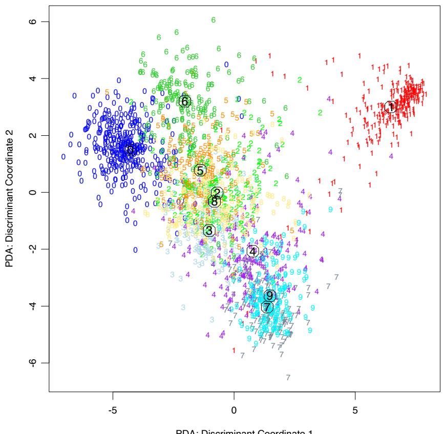
PDA: Discriminant Coordinate 1

FIGURE 12.12. The first two penalized canonical variates, evaluated for the test data. The circles indicate the class centroids. The first coordinate contrasts mainly 0’s and 1’s, while the second contrasts 6’s and 7/9’s.

examples are discussed in more detail in Hastie et al. (1995), who also show that the regularization improves the classification performance of LDA on independent test data by a factor of around 25% in the cases they tried.

12.7 Mixture Discriminant Analysis

Linear discriminant analysis can be viewed as a prototype classifier. Each class is represented by its centroid, and we classify to the closest using an appropriate metric. In many situations a single prototype is not sufficient to represent inhomogeneous classes, and mixture models are more appropriate. In this section we review Gaussian mixture models and show how they can be generalized via the FDA and PDA methods discussed earlier. A Gaussian mixture model for the kth class has density

\[P(X|G=k) = \sum\_{r=1}^{R\_k} \pi\_{kr} \phi(X; \mu\_{kr}, \Sigma),\tag{12.59}\]

where the mixing proportions πkr sum to one. This has R^k prototypes for the kth class, and in our specification, the same covariance matrix Σ is used as the metric throughout. Given such a model for each class, the class posterior probabilities are given by

\[P(G=k|X=x) = \frac{\sum\_{r=1}^{R\_k} \pi\_{kr} \phi(X; \mu\_{kr}, \Sigma) \Pi\_k}{\sum\_{\ell=1}^{K} \sum\_{r=1}^{R\_\ell} \pi\_{\ell r} \phi(X; \mu\_{\ell r}, \Sigma) \Pi\_\ell},\tag{12.60}\]

where Π^k represent the class prior probabilities.

We saw these calculations for the special case of two components in Chapter 8. As in LDA, we estimate the parameters by maximum likelihood, using the joint log-likelihood based on P(G, X):

\[\sum\_{k=1}^{K} \sum\_{g\_i=k} \log \left[ \sum\_{r=1}^{R\_k} \pi\_{kr} \phi(x\_i; \mu\_{kr}, \Sigma) \Pi\_k \right]. \tag{12.61}\]

The sum within the log makes this a rather messy optimization problem if tackled directly. The classical and natural method for computing the maximum-likelihood estimates (MLEs) for mixture distributions is the EM algorithm (Dempster et al., 1977), which is known to possess good convergence properties. EM alternates between the two steps:

450 12. Flexible Discriminants

E-step: Given the current parameters, compute the responsibility of subclass ckr within class k for each of the class-k observations (gⁱ = k):

\[W(c\_{kr}|x\_i, g\_i) = \frac{\pi\_{kr}\phi(x\_i; \mu\_{kr}, \Sigma)}{\sum\_{\ell=1}^{R\_k} \pi\_{k\ell}\phi(x\_i; \mu\_{k\ell}, \Sigma)}. \tag{12.62}\]

M-step: Compute the weighted MLEs for the parameters of each of the component Gaussians within each of the classes, using the weights from the E-step.

In the E-step, the algorithm apportions the unit weight of an observation in class k to the various subclasses assigned to that class. If it is close to the centroid of a particular subclass, and far from the others, it will receive a mass close to one for that subclass. On the other hand, observations halfway between two subclasses will get approximately equal weight for both.

In the M-step, an observation in class k is used R^k times, to estimate the parameters in each of the R^k component densities, with a different weight for each. The EM algorithm is studied in detail in Chapter 8. The algorithm requires initialization, which can have an impact, since mixture likelihoods are generally multimodal. Our software (referenced in the Computational Considerations on page 455) allows several strategies; here we describe the default. The user supplies the number R^k of subclasses per class. Within class k, a k-means clustering model, with multiple random starts, is fitted to the data. This partitions the observations into R^k disjoint groups, from which an initial weight matrix, consisting of zeros and ones, is created.

Our assumption of an equal component covariance matrix Σ throughout buys an additional simplicity; we can incorporate rank restrictions in the mixture formulation just like in LDA. To understand this, we review a littleknown fact about LDA. The rank-L LDA fit (Section 4.3.3) is equivalent to the maximum-likelihood fit of a Gaussian model,where the different mean vectors in each class are confined to a rank-L subspace of IR^p (Exercise 4.8). We can inherit this property for the mixture model, and maximize the loglikelihood (12.61) subject to rank constraints on all the # ^k R^k centroids: rank{µkℓ} = L.

Again the EM algorithm is available, and the M-step turns out to be a weighted version of LDA, with R = #^{K k}=1 R^k “classes.” Furthermore, we can use optimal scoring as before to solve the weighted LDA problem, which allows us to use a weighted version of FDA or PDA at this stage. One would expect, in addition to an increase in the number of “classes,” a similar increase in the number of “observations” in the kth class by a factor of Rk. It turns out that this is not the case if linear operators are used for the optimal scoring regression. The enlarged indicator Y matrix collapses in this case to a blurred response matrix Z, which is intuitively pleasing. For example, suppose there are K = 3 classes, and R^k = 3 subclasses per class. Then Z might be

\[\begin{array}{l} g\_1 = 2 \\ g\_2 = 1 \\ g\_3 = 1 \\ g\_4 = 3 \\ g\_5 = 2 \\ \vdots \\ g\_N = 3 \end{array} \left( \begin{array}{l} 0 & 0 & 0 & 0 & 0.3 & 0.5 & 0.2 & 0 & 0 & 0 \\ 0.9 & 0.1 & 0.0 & 0 & 0 & 0 & 0 & 0 \\ 0.1 & 0.8 & 0.1 & 0 & 0 & 0 & 0 & 0 \\ 0 & 0 & 0 & 0 & 0 & 0 & 0.5 & 0.4 & 0.1 \\ 0 & 0 & 0 & 0.7 & 0.1 & 0.2 & 0 & 0 & 0 \\ & & & & & & \\ & & & & & & \\ g\_N = 3 \end{array} \right), \tag{12.63}\]

where the entries in a class-k row correspond to W(ckr|x, gi). The remaining steps are the same:

\[\begin{aligned} \hat{\mathbf{Z}} &= \mathbf{S} \mathbf{Z} \\ \mathbf{Z}^T \hat{\mathbf{Z}} &= \boldsymbol{\Theta} \mathbf{D} \boldsymbol{\Theta}^T \\ \text{Update } \pi \text{s and IIs} \end{aligned} \quad \text{ $M$ -step of MAD.}\]

These simple modifications add considerable flexibility to the mixture model:

• The dimension reduction step in LDA, FDA or PDA is limited by the number of classes; in particular, for K = 2 classes no reduction is possible. MDA substitutes subclasses for classes, and then allows us to look at low-dimensional views of the subspace spanned by these subclass centroids. This subspace will often be an important one for discrimination.
• By using FDA or PDA in the M-step, we can adapt even more to particular situations. For example, we can fit MDA models to digitized analog signals and images, with smoothness constraints built in.

Figure 12.13 compares FDA and MDA on the mixture example.

12.7.1 Example: Waveform Data

We now illustrate some of these ideas on a popular simulated example, taken from Breiman et al. (1984, pages 49–55), and used in Hastie and Tibshirani (1996b) and elsewhere. It is a three-class problem with 21 variables, and is considered to be a difficult pattern recognition problem. The predictors are defined by

\[\begin{array}{rclrcl}X\_j &=& Uh\_1(j) + (1-U)h\_2(j) + \epsilon\_j & \text{Class 1,} \\ X\_j &=& Uh\_1(j) + (1-U)h\_3(j) + \epsilon\_j & \text{Class 2,} \\ X\_j &=& Uh\_2(j) + (1-U)h\_3(j) + \epsilon\_j & \text{Class 3,} \end{array} \tag{12.64}\]

where j = 1, 2,…, 21, U is uniform on (0, 1), ϵ^j are standard normal variates, and the h^ℓ are the shifted triangular waveforms: h1(j) = max(6 −

FIGURE 12.14. Some examples of the waveforms generated from model (12.64) before the Gaussian noise is added.

|j − 11|, 0), h2(j) = h1(j − 4) and h3(j) = h1(j + 4). Figure 12.14 shows some example waveforms from each class.

Table 12.4 shows the results of MDA applied to the waveform data, as well as several other methods from this and other chapters. Each training sample has 300 observations, and equal priors were used, so there are roughly 100 observations in each class. We used test samples of size 500. The two MDA models are described in the caption.

Figure 12.15 shows the leading canonical variates for the penalized MDA model, evaluated at the test data. As we might have guessed, the classes appear to lie on the edges of a triangle. This is because the h^j (i) are represented by three points in 21-space, thereby forming vertices of a triangle, and each class is represented as a convex combination of a pair of vertices, and hence lie on an edge. Also it is clear visually that all the information lies in the first two dimensions; the percentage of variance explained by the first two coordinates is 99.8%, and we would lose nothing by truncating the solution there. The Bayes risk for this problem has been estimated to be about 0.14 (Breiman et al., 1984). MDA comes close to the optimal rate, which is not surprising since the structure of the MDA model is similar to the generating model.

454 12. Flexible Discriminants

TABLE 12.4. Results for waveform data. The values are averages over ten simulations, with the standard error of the average in parentheses. The five entries above the line are taken from Hastie et al. (1994). The first model below the line is MDA with three subclasses per class. The next line is the same, except that the discriminant coefficients are penalized via a roughness penalty to effectively 4df. The third is the corresponding penalized LDA or PDA model.

Technique	Error Rates
	Training	Test
LDA	0.121(0.006)	0.191(0.006)
QDA	0.039(0.004)	0.205(0.006)
CART	0.072(0.003)	0.289(0.004)
FDA/MARS (degree = 1)	0.100(0.006)	0.191(0.006)
FDA/MARS (degree = 2)	0.068(0.004)	0.215(0.002)
MDA (3 subclasses)	0.087(0.005)	0.169(0.006)
MDA (3 subclasses, penalized 4 df)	0.137(0.006)	0.157(0.005)
PDA (penalized 4 df)	0.150(0.005)	0.171(0.005)
Bayes		0.140

FIGURE 12.15. Some two-dimensional views of the MDA model fitted to a sample of the waveform model. The points are independent test data, projected on to the leading two canonical coordinates (left panel), and the third and fourth (right panel). The subclass centers are indicated.

Computational Considerations

With N training cases, p predictors, and m support vectors, the support vector machine requires ^{m3 +} mN ⁺ mpN operations, assuming ^{m ≈ N}. They do not scale well with N, although computational shortcuts are available (Platt, 1999). Since these are evolving rapidly, the reader is urged to search the web for the latest technology.

LDA requires N p² + p³ operations, as does PDA. The complexity of FDA depends on the regression method used. Many techniques are linear in N, such as additive models and MARS. General splines and kernel-based regression methods will typically require N³ operations.

Software is available for fitting FDA, PDA and MDA models in the R package mda, which is also available in S-PLUS.

Bibliographic Notes

The theory behind support vector machines is due to Vapnik and is described in Vapnik (1996). There is a burgeoning literature on SVMs; an online bibliography, created and maintained by Alex Smola and Bernhard Sch¨olkopf, can be found at:

http://www.kernel-machines.org.

Our treatment is based on Wahba et al. (2000) and Evgeniou et al. (2000), and the tutorial by Burges (Burges, 1998).

Linear discriminant analysis is due to Fisher (1936) and Rao (1973). The connection with optimal scoring dates back at least to Breiman and Ihaka (1984), and in a simple form to Fisher (1936). There are strong connections with correspondence analysis (Greenacre, 1984). The description of flexible, penalized and mixture discriminant analysis is taken from Hastie et al. (1994), Hastie et al. (1995) and Hastie and Tibshirani (1996b), and all three are summarized in Hastie et al. (1998); see also Ripley (1996).

Exercises

Ex. 12.1 Show that the criteria (12.25) and (12.8) are equivalent.

Ex. 12.2 Show that the solution to (12.29) is the same as the solution to (12.25) for a particular kernel.

Ex. 12.3 Consider a modification to (12.43) where you do not penalize the constant. Formulate the problem, and characterize its solution.

Ex. 12.4 Suppose you perform a reduced-subspace linear discriminant analysis for a K-group problem. You compute the canonical variables of dimension ^{L ≤ K −} 1 given by ^{z = UT x}, where ^U is the ^{p × L} matrix of discriminant coefficients, and p>K is the dimension of x.

1. If L = K − 1 show that

\[\left\| \left| z - \bar{z}\_k \right| \right\|^2 - \left\| z - \bar{z}\_{k'} \right\|^2 = \left\| x - \bar{x}\_k \right\|\_W^2 - \left\| x - \bar{x}\_{k'} \right\|\_W^2,\]

where ∥·∥^W denotes Mahalanobis distance with respect to the covariance W.

2. If L<K − 1, show that the same expression on the left measures the difference in Mahalanobis squared distances for the distributions projected onto the subspace spanned by U.

Ex. 12.5 The data in phoneme.subset, available from this book’s website

http://www-stat.stanford.edu/ElemStatLearn

consists of digitized log-periodograms for phonemes uttered by 60 speakers, each speaker having produced phonemes from each of five classes. It is appropriate to plot each vector of 256 “features” against the frequencies 0–255.

• 1. Produce a separate plot of all the phoneme curves against frequency for each class.
• 2. You plan to use a nearest prototype classification scheme to classify the curves into phoneme classes. In particular, you will use a K-means clustering algorithm in each class (kmeans() in R), and then classify observations to the class of the closest cluster center. The curves are high-dimensional and you have a rather small sample-size-to-variables ratio. You decide to restrict all the prototypes to be smooth functions of frequency. In particular, you decide to represent each prototype m as m = Bθ where B is a 256 × J matrix of natural spline basis functions with J knots uniformly chosen in (0, 255) and boundary knots at 0 and 255. Describe how to proceed analytically, and in particular, how to avoid costly high-dimensional fitting procedures. (Hint: It may help to restrict B to be orthogonal.)
• 3. Implement your procedure on the phoneme data, and try it out. Divide the data into a training set and a test set (50-50), making sure that speakers are not split across sets (why?). Use K = 1, 3, 5, 7 centers per class, and for each use J = 5, 10, 15 knots (taking care to start the K-means procedure at the same starting values for each value of J), and compare the results.

Ex. 12.6 Suppose that the regression procedure used in FDA (Section 12.5.1) is a linear expansion of basis functions hm(x), m = 1,…,M. Let D^π = Y^T Y/N be the diagonal matrix of class proportions.

1. Show that the optimal scoring problem (12.52) can be written in vector notation as

\[\min\_{\theta, \beta} \left\| \mathbf{Y}\theta - \mathbf{H}\beta \right\|^2,\tag{12.65}\]

where θ is a vector of K real numbers, and H is the N × M matrix of evaluations h^j (xi).

• 2. Suppose that the normalization on θ is θ^T Dπ1 = 0 and θ^T Dπθ = 1. Interpret these normalizations in terms of the original scored θ(gi).
• 3. Show that, with this normalization, (12.65) can be partially optimized w.r.t. β, and leads to

\[\max\_{\boldsymbol{\theta}} \boldsymbol{\theta}^T \mathbf{S} \boldsymbol{\theta}, \tag{12.66}\]

subject to the normalization constraints, where S is the projection operator corresponding to the basis matrix H.

• 4. Suppose that the h^j include the constant function. Show that the largest eigenvalue of S is 1.
• 5. Let Θ be a K × K matrix of scores (in columns), and suppose the normalization is Θ^T DπΘ = I. Show that the solution to (12.53) is given by the complete set of eigenvectors of S; the first eigenvector is trivial, and takes care of the centering of the scores. The remainder characterize the optimal scoring solution.

Ex. 12.7 Derive the solution to the penalized optimal scoring problem (12.57).

Ex. 12.8 Show that coefficients β^ℓ found by optimal scoring are proportional to the discriminant directions ν^ℓ found by linear discriminant analysis.

Ex. 12.9 Let ^{Yˆ =} XB^ˆ be the fitted ^{N × K} indicator response matrix after linear regression on the N ×p matrix X, where p>K. Consider the reduced features x^{∗ i = Bˆ T x}i. Show that LDA using ^{x∗ i} is equivalent to LDA in the original space.

Ex. 12.10 Kernels and linear discriminant analysis. Suppose you wish to carry out a linear discriminant analysis (two classes) using a vector of transformations of the input variables h(x). Since h(x) is high-dimensional, you will use a regularized within-class covariance matrix W^h + γI. Show that the model can be estimated using only the inner products K(xi, xi′ ) = ⟨h(xi), h(xi′ )⟩. Hence the kernel property of support vector machines is also shared by regularized linear discriminant analysis.

Ex. 12.11 The MDA procedure models each class as a mixture of Gaussians. Hence each mixture center belongs to one and only one class. A more general model allows each mixture center to be shared by all classes. We take the joint density of labels and features to be

458 12. Flexible Discriminants

\[P(G,X) = \sum\_{r=1}^{R} \pi\_r P\_r(G,X),\tag{12.67}\]

a mixture of joint densities. Furthermore we assume

\[P\_r(G, X) = P\_r(G) \phi(X; \mu\_r, \Sigma). \tag{12.68}\]

This model consists of regions centered at µr, and for each there is a class profile Pr(G). The posterior class distribution is given by

\[P(G=k|X=x) = \frac{\sum\_{r=1}^{R} \pi\_r P\_r(G=k) \phi(x; \mu\_r, \Sigma)}{\sum\_{r=1}^{R} \pi\_r \phi(x; \mu\_r, \Sigma)},\tag{12.69}\]

where the denominator is the marginal distribution P(X).

1. Show that this model (called MDA2) can be viewed as a generalization of MDA since

\[P(X|G=k) = \frac{\sum\_{r=1}^{R} \pi\_r P\_r(G=k) \phi(x; \mu\_r, \Sigma)}{\sum\_{r=1}^{R} \pi\_r P\_r(G=k)},\tag{12.70}\]

where πrk = πrPr(G = k)/ #^{R r}=1 πrPr(G = k) corresponds to the mixing proportions for the kth class.

• 2. Derive the EM algorithm for MDA2.
• 3. Show that if the initial weight matrix is constructed as in MDA, involving separate k-means clustering in each class, then the algorithm for MDA2 is identical to the original MDA procedure.

This is page 459 Printer: Opaque this

13 Prototype Methods and Nearest-Neighbors

13.1 Introduction

In this chapter we discuss some simple and essentially model-free methods for classification and pattern recognition. Because they are highly unstructured, they typically are not useful for understanding the nature of the relationship between the features and class outcome. However, as black box prediction engines, they can be very effective, and are often among the best performers in real data problems. The nearest-neighbor technique can also be used in regression; this was touched on in Chapter 2 and works reasonably well for low-dimensional problems. However, with high-dimensional features, the bias–variance tradeoff does not work as favorably for nearestneighbor regression as it does for classification.

13.2 Prototype Methods

Throughout this chapter, our training data consists of the N pairs (x1, g1), …, (xn, g^N ) where gⁱ is a class label taking values in {1, 2,…,K}. Prototype methods represent the training data by a set of points in feature space. These prototypes are typically not examples from the training sample, except in the case of 1-nearest-neighbor classification discussed later.

Each prototype has an associated class label, and classification of a query point x is made to the class of the closest prototype. “Closest” is usually defined by Euclidean distance in the feature space, after each feature has

460 13. Prototypes and Nearest-Neighbors

been standardized to have overall mean 0 and variance 1 in the training sample. Euclidean distance is appropriate for quantitative features. We discuss distance measures between qualitative and other kinds of feature values in Chapter 14.

These methods can be very effective if the prototypes are well positioned to capture the distribution of each class. Irregular class boundaries can be represented, with enough prototypes in the right places in feature space. The main challenge is to figure out how many prototypes to use and where to put them. Methods differ according to the number and way in which prototypes are selected.

13.2.1 K-means Clustering

K-means clustering is a method for finding clusters and cluster centers in a set of unlabeled data. One chooses the desired number of cluster centers, say R, and the K-means procedure iteratively moves the centers to minimize the total within cluster variance.¹ Given an initial set of centers, the Kmeans algorithm alternates the two steps:

• for each center we identify the subset of training points (its cluster) that is closer to it than any other center;
• the means of each feature for the data points in each cluster are computed, and this mean vector becomes the new center for that cluster.

These two steps are iterated until convergence. Typically the initial centers are R randomly chosen observations from the training data. Details of the K-means procedure, as well as generalizations allowing for different variable types and more general distance measures, are given in Chapter 14.

To use K-means clustering for classification of labeled data, the steps are:

• apply K-means clustering to the training data in each class separately, using R prototypes per class;
• assign a class label to each of the K × R prototypes;
• classify a new feature x to the class of the closest prototype.

Figure 13.1 (upper panel) shows a simulated example with three classes and two features. We used R = 5 prototypes per class, and show the classification regions and the decision boundary. Notice that a number of the

¹The “K” in K-means refers to the number of cluster centers. Since we have already reserved K to denote the number of classes, we denote the number of clusters by R.

462 13. Prototypes and Nearest-Neighbors

				Algorithm 13.1 Learning Vector Quantization—LVQ.
–	–	–	–	————————————————–	–

• 1. Choose R initial prototypes for each class: m1(k), m2(k),…,mR(k), k = 1, 2,…,K, for example, by sampling R training points at random from each class.
• 2. Sample a training point xⁱ randomly (with replacement), and let (j, k) index the closest prototype m^j (k) to xi.
  • 1. If gⁱ = k (i.e., they are in the same class), move the prototype towards the training point:

\[m\_j(k) \leftarrow m\_j(k) + \epsilon(x\_i - m\_j(k)),\]

where ϵ is the learning rate.

2. If gⁱ ̸= k (i.e., they are in different classes), move the prototype away from the training point:

\[m\_j(k) \leftarrow m\_j(k) - \epsilon(x\_i - m\_j(k)).\]

3. Repeat step 2, decreasing the learning rate ϵ with each iteration towards zero.

prototypes are near the class boundaries, leading to potential misclassification errors for points near these boundaries. This results from an obvious shortcoming with this method: for each class, the other classes do not have a say in the positioning of the prototypes for that class. A better approach, discussed next, uses all of the data to position all prototypes.

13.2.2 Learning Vector Quantization

In this technique due to Kohonen (1989), prototypes are placed strategically with respect to the decision boundaries in an ad-hoc way. LVQ is an online algorithm—observations are processed one at a time.

The idea is that the training points attract prototypes of the correct class, and repel other prototypes. When the iterations settle down, prototypes should be close to the training points in their class. The learning rate ϵ is decreased to zero with each iteration, following the guidelines for stochastic approximation learning rates (Section 11.4.)

Figure 13.1 (lower panel) shows the result of LVQ, using the K-means solution as starting values. The prototypes have tended to move away from the decision boundaries, and away from prototypes of competing classes.

The procedure just described is actually called LVQ1. Modifications (LVQ2, LVQ3, etc.) have been proposed, that can sometimes improve performance. A drawback of learning vector quantization methods is the fact that they are defined by algorithms, rather than optimization of some fixed criteria; this makes it difficult to understand their properties.

13.2.3 Gaussian Mixtures

The Gaussian mixture model can also be thought of as a prototype method, similar in spirit to K-means and LVQ. We discuss Gaussian mixtures in some detail in Sections 6.8, 8.5 and 12.7. Each cluster is described in terms of a Gaussian density, which has a centroid (as in K-means), and a covariance matrix. The comparison becomes crisper if we restrict the component Gaussians to have a scalar covariance matrix (Exercise 13.1). The two steps of the alternating EM algorithm are very similar to the two steps in Kmeans:

• In the E-step, each observation is assigned a responsibility or weight for each cluster, based on the likelihood of each of the corresponding Gaussians. Observations close to the center of a cluster will most likely get weight 1 for that cluster, and weight 0 for every other cluster. Observations half-way between two clusters divide their weight accordingly.
• In the M-step, each observation contributes to the weighted means (and covariances) for every cluster.

As a consequence, the Gaussian mixture model is often referred to as a soft clustering method, while K-means is hard.

Similarly, when Gaussian mixture models are used to represent the feature density in each class, it produces smooth posterior probabilities ˆp(x) = {pˆ1(x),…, pˆK(x)} for classifying x (see (12.60) on page 449.) Often this is interpreted as a soft classification, while in fact the classification rule is Gˆ(x) = arg max^k pˆk(x). Figure 13.2 compares the results of K-means and Gaussian mixtures on the simulated mixture problem of Chapter 2. We see that although the decision boundaries are roughly similar, those for the mixture model are smoother (although the prototypes are in approximately the same positions.) We also see that while both procedures devote a blue prototype (incorrectly) to a region in the northwest, the Gaussian mixture classifier can ultimately ignore this region, while K-means cannot. LVQ gave very similar results to K-means on this example, and is not shown.

13.3 k-Nearest-Neighbor Classifiers

These classifiers are memory-based, and require no model to be fit. Given a query point x0, we find the k training points x(r), r = 1,…,k closest in distance to x0, and then classify using majority vote among the k neighbors.

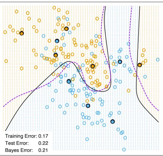
Ties are broken at random. For simplicity we will assume that the features are real-valued, and we use Euclidean distance in feature space:

\[d\_{(i)} = ||x\_{(i)} - x\_0||.\tag{13.1}\]

Typically we first standardize each of the features to have mean zero and variance 1, since it is possible that they are measured in different units. In Chapter 14 we discuss distance measures appropriate for qualitative and ordinal features, and how to combine them for mixed data. Adaptively chosen distance metrics are discussed later in this chapter.

Despite its simplicity, k-nearest-neighbors has been successful in a large number of classification problems, including handwritten digits, satellite image scenes and EKG patterns. It is often successful where each class has many possible prototypes, and the decision boundary is very irregular. Figure 13.3 (upper panel) shows the decision boundary of a 15-nearestneighbor classifier applied to the three-class simulated data. The decision boundary is fairly smooth compared to the lower panel, where a 1-nearestneighbor classifier was used. There is a close relationship between nearestneighbor and prototype methods: in 1-nearest-neighbor classification, each training point is a prototype.

Figure 13.4 shows the training, test and tenfold cross-validation errors as a function of the neighborhood size, for the two-class mixture problem. Since the tenfold CV errors are averages of ten numbers, we can estimate a standard error.

Because it uses only the training point closest to the query point, the bias of the 1-nearest-neighbor estimate is often low, but the variance is high. A famous result of Cover and Hart (1967) shows that asymptotically the error rate of the 1-nearest-neighbor classifier is never more than twice the Bayes rate. The rough idea of the proof is as follows (using squared-error loss). We assume that the query point coincides with one of the training points, so that the bias is zero. This is true asymptotically if the dimension of the feature space is fixed and the training data fills up the space in a dense fashion. Then the error of the Bayes rule is just the variance of a Bernoulli random variate (the target at the query point), while the error of 1-nearest-neighbor rule is twice the variance of a Bernoulli random variate, one contribution each for the training and query targets.

We now give more detail for misclassification loss. At x let k^∗ be the dominant class, and pk(x) the true conditional probability for class k. Then

\[\text{Bayes error} \quad = \quad 1 - p\_{k^\*} (x), \tag{13.2}\]

\[1\text{-nearest-neighbor error}\,\,=\,\,\sum\_{k=1}^{K}p\_k(x)(1-p\_k(x)),\tag{13.3}\]

\[\geq \begin{array}{c} k=1\\ 1-p\_{k^\*}(x). \end{array} \tag{13.4}\]

The asymptotic 1-nearest-neighbor error rate is that of a random rule; we pick both the classification and the test point at random with probabili-

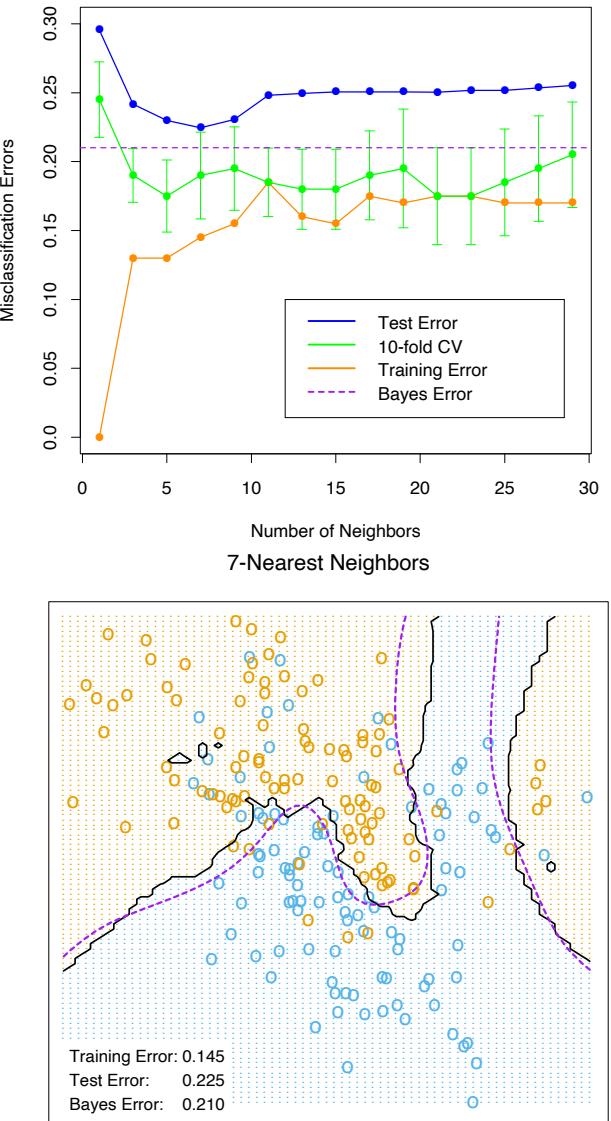
468 13. Prototypes and Nearest-Neighbors

ties pk(x), k = 1,…,K. For K = 2 the 1-nearest-neighbor error rate is 2pk^∗ (x)(1 − pk^∗ (x)) ≤ 2(1 − pk^∗ (x)) (twice the Bayes error rate). More generally, one can show (Exercise 13.3)

\[\sum\_{k=1}^{K} p\_k(x)(1 - p\_k(x)) \le 2(1 - p\_{k^\*}(x)) - \frac{K}{K - 1}(1 - p\_{k^\*}(x))^2. \tag{13.5}\]

Many additional results of this kind have been derived; Ripley (1996) summarizes a number of them.

This result can provide a rough idea about the best performance that is possible in a given problem. For example, if the 1-nearest-neighbor rule has a 10% error rate, then asymptotically the Bayes error rate is at least 5%. The kicker here is the asymptotic part, which assumes the bias of the nearest-neighbor rule is zero. In real problems the bias can be substantial. The adaptive nearest-neighbor rules, described later in this chapter, are an attempt to alleviate this bias. For simple nearest-neighbors, the bias and variance characteristics can dictate the optimal number of near neighbors for a given problem. This is illustrated in the next example.

13.3.1 Example: A Comparative Study

We tested the nearest-neighbors, K-means and LVQ classifiers on two simulated problems. There are 10 independent features X^j , each uniformly distributed on [0, 1]. The two-class 0-1 target variable is defined as follows:

\[\begin{aligned} Y &= I\left(X\_1 > \frac{1}{2}\right); \quad \text{problem 1: "easy"},\\ Y &= I\left(\text{sign}\left\{\prod\_{j=1}^3 \left(X\_j - \frac{1}{2}\right)\right\} > 0\right); \quad \text{problem 2: "differenti."} \end{aligned} \tag{13.6}\]

Hence in the first problem the two classes are separated by the hyperplane X¹ = 1/2; in the second problem, the two classes form a checkerboard pattern in the hypercube defined by the first three features. The Bayes error rate is zero in both problems. There were 100 training and 1000 test observations.

Figure 13.5 shows the mean and standard error of the misclassification error for nearest-neighbors, K-means and LVQ over ten realizations, as the tuning parameters are varied. We see that K-means and LVQ give nearly identical results. For the best choices of their tuning parameters, K-means and LVQ outperform nearest-neighbors for the first problem, and they perform similarly for the second problem. Notice that the best value of each tuning parameter is clearly situation dependent. For example 25 nearest-neighbors outperforms 1-nearest-neighbor by a factor of 70% in the

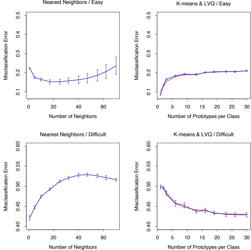
FIGURE 13.5. Mean ± one standard error of misclassification error for nearest-neighbors, K-means (blue) and LVQ (red) over ten realizations for two simulated problems: “easy” and “difficult,” described in the text.

470 13. Prototypes and Nearest-Neighbors

FIGURE 13.6. The first four panels are LANDSAT images for an agricultural area in four spectral bands, depicted by heatmap shading. The remaining two panels give the actual land usage (color coded) and the predicted land usage using a five-nearest-neighbor rule described in the text.

first problem, while 1-nearest-neighbor is best in the second problem by a factor of 18%. These results underline the importance of using an objective, data-based method like cross-validation to estimate the best value of a tuning parameter (see Figure 13.4 and Chapter 7).

13.3.2 Example: k-Nearest-Neighbors and Image Scene Classification

The STATLOG project (Michie et al., 1994) used part of a LANDSAT image as a benchmark for classification (82×100 pixels). Figure 13.6 shows four heat-map images, two in the visible spectrum and two in the infrared, for an area of agricultural land in Australia. Each pixel has a class label from the 7-element set G = {red soil, cotton, vegetation stubble, mixture, gray soil, damp gray soil, very damp gray soil}, determined manually by research assistants surveying the area. The lower middle panel shows the actual land usage, shaded by different colors to indicate the classes. The objective is to classify the land usage at a pixel, based on the information in the four spectral bands.

Five-nearest-neighbors produced the predicted map shown in the bottom right panel, and was computed as follows. For each pixel we extracted an 8-neighbor feature map—the pixel itself and its 8 immediate neighbors

N	N	N
N	X	N
N	N	N

FIGURE 13.7. A pixel and its 8-neighbor feature map.

(see Figure 13.7). This is done separately in the four spectral bands, giving (1+ 8)×4 = 36 input features per pixel. Then five-nearest-neighbors classification was carried out in this 36-dimensional feature space. The resulting test error rate was about 9.5% (see Figure 13.8). Of all the methods used in the STATLOG project, including LVQ, CART, neural networks, linear discriminant analysis and many others, k-nearest-neighbors performed best on this task. Hence it is likely that the decision boundaries in IR³⁶ are quite irregular.

13.3.3 Invariant Metrics and Tangent Distance

In some problems, the training features are invariant under certain natural transformations. The nearest-neighbor classifier can exploit such invariances by incorporating them into the metric used to measure the distances between objects. Here we give an example where this idea was used with great success, and the resulting classifier outperformed all others at the time of its development (Simard et al., 1993).

The problem is handwritten digit recognition, as discussed is Chapter 1 and Section 11.7. The inputs are grayscale images with 16 × 16 = 256 pixels; some examples are shown in Figure 13.9. At the top of Figure 13.10, a “3” is shown, in its actual orientation (middle) and rotated 7.5◦ and 15◦ in either direction. Such rotations can often occur in real handwriting, and it is obvious to our eye that this “3” is still a “3” after small rotations. Hence we want our nearest-neighbor classifier to consider these two “3”s to be close together (similar). However the 256 grayscale pixel values for a rotated “3” will look quite different from those in the original image, and hence the two objects can be far apart in Euclidean distance in IR256.

We wish to remove the effect of rotation in measuring distances between two digits of the same class. Consider the set of pixel values consisting of the original “3” and its rotated versions. This is a one-dimensional curve in IR256, depicted by the green curve passing through the “3” in Figure 13.10. Figure 13.11 shows a stylized version of IR256, with two images indicated by xⁱ and xi′ . These might be two different “3”s, for example. Through each image we have drawn the curve of rotated versions of that image, called

STATLOG results

FIGURE 13.8. Test-error performance for a number of classifiers, as reported by the STATLOG project. The entry DANN is a variant of k-nearest neighbors, using an adaptive metric (Section 13.4.2).

FIGURE 13.9. Examples of grayscale images of handwritten digits.

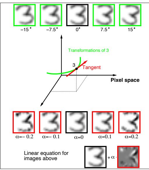
FIGURE 13.10. The top row shows a ” 3” in its original orientation (middle) and rotated versions of it. The green curve in the middle of the figure depicts this set of rotated ” 3” in 256-dimensional space. The red line is the tangent line to the curve at the original image, with some ” 3”s on this tangent line, and its equation shown at the bottom of the figure.

invariance manifolds in this context. Now, rather than using the usual Euclidean distance between the two images, we use the shortest distance between the two curves. In other words, the distance between the two images is taken to be the shortest Euclidean distance between any rotated version of first image, and any rotated version of the second image. This distance is called an invariant metric.

In principle one could carry out 1-nearest-neighbor classification using this invariant metric. However there are two problems with it. First, it is very difficult to calculate for real images. Second, it allows large transformations that can lead to poor performance. For example a “6” would be considered close to a “9” after a rotation of 180◦. We need to restrict attention to small rotations.

The use of tangent distance solves both of these problems. As shown in Figure 13.10, we can approximate the invariance manifold of the image “3” by its tangent at the original image. This tangent can be computed by estimating the direction vector from small rotations of the image, or by more sophisticated spatial smoothing methods (Exercise 13.4.) For large rotations, the tangent image no longer looks like a “3,” so the problem with large transformations is alleviated.

474 13. Prototypes and Nearest-Neighbors

FIGURE 13.11. Tangent distance computation for two images xⁱ and xi′ . Rather than using the Euclidean distance between xⁱ and xi′ , or the shortest distance between the two curves, we use the shortest distance between the two tangent lines.

The idea then is to compute the invariant tangent line for each training image. For a query image to be classified, we compute its invariant tangent line, and find the closest line to it among the lines in the training set. The class (digit) corresponding to this closest line is our predicted class for the query image. In Figure 13.11 the two tangent lines intersect, but this is only because we have been forced to draw a two-dimensional representation of the actual 256-dimensional situation. In IR²⁵⁶ the probability of two such lines intersecting is effectively zero.

Now a simpler way to achieve this invariance would be to add into the training set a number of rotated versions of each training image, and then just use a standard nearest-neighbor classifier. This idea is called “hints” in Abu-Mostafa (1995), and works well when the space of invariances is small. So far we have presented a simplified version of the problem. In addition to rotation, there are six other types of transformations under which we would like our classifier to be invariant. There are translation (two directions), scaling (two directions), sheer, and character thickness. Hence the curves and tangent lines in Figures 13.10 and 13.11 are actually 7-dimensional manifolds and hyperplanes. It is infeasible to add transformed versions of each training image to capture all of these possibilities. The tangent manifolds provide an elegant way of capturing the invariances.

Table 13.1 shows the test misclassification error for a problem with 7291 training images and 2007 test digits (the U.S. Postal Services database), for a carefully constructed neural network, and simple 1-nearest-neighbor and

Method	Error rate
Neural-net	0.049
1-nearest-neighbor/Euclidean distance	0.055
1-nearest-neighbor/tangent distance	0.026

TABLE 13.1. Test error rates for the handwritten ZIP code problem.

tangent distance 1-nearest-neighbor rules. The tangent distance nearestneighbor classifier works remarkably well, with test error rates near those for the human eye (this is a notoriously difficult test set). In practice, it turned out that nearest-neighbors are too slow for online classification in this application (see Section 13.5), and neural network classifiers were subsequently developed to mimic it.

13.4 Adaptive Nearest-Neighbor Methods

When nearest-neighbor classification is carried out in a high-dimensional feature space, the nearest neighbors of a point can be very far away, causing bias and degrading the performance of the rule.

To quantify this, consider N data points uniformly distributed in the unit cube [−^{1 2} , ¹ 2 ] ^p. Let R be the radius of a 1-nearest-neighborhood centered at the origin. Then

\[\text{median}(R) = v\_p^{-1/p} \left( 1 - \frac{1}{2}^{1/N} \right)^{1/p},\tag{13.7}\]

where vpr^p is the volume of the sphere of radius r in p dimensions. Figure 13.12 shows the median radius for various training sample sizes and dimensions. We see that median radius quickly approaches 0.5, the distance to the edge of the cube.

What can be done about this problem? Consider the two-class situation in Figure 13.13. There are two features, and a nearest-neighborhood at a query point is depicted by the circular region. Implicit in near-neighbor classification is the assumption that the class probabilities are roughly constant in the neighborhood, and hence simple averages give good estimates. However, in this example the class probabilities vary only in the horizontal direction. If we knew this, we would stretch the neighborhood in the vertical direction, as shown by the tall rectangular region. This will reduce the bias of our estimate and leave the variance the same.

In general, this calls for adapting the metric used in nearest-neighbor classification, so that the resulting neighborhoods stretch out in directions for which the class probabilities don’t change much. In high-dimensional feature space, the class probabilities might change only a low-dimensional subspace and hence there can be considerable advantage to adapting the metric.

FIGURE 13.12. Median radius of a 1-nearest-neighborhood, for uniform data with N observations in p dimensions.

FIGURE 13.13. The points are uniform in the cube, with the vertical line separating class red and green. The vertical strip denotes the 5-nearest-neighbor region using only the horizontal coordinate to find the nearest-neighbors for the target point (solid dot). The sphere shows the 5-nearest-neighbor region using both coordinates, and we see in this case it has extended into the class-red region (and is dominated by the wrong class in this instance).

Friedman (1994a) proposed a method in which rectangular neighborhoods are found adaptively by successively carving away edges of a box containing the training data. Here we describe the discriminant adaptive nearest-neighbor (DANN) rule of Hastie and Tibshirani (1996a). Earlier, related proposals appear in Short and Fukunaga (1981) and Myles and Hand (1990).

At each query point a neighborhood of say 50 points is formed, and the class distribution among the points is used to decide how to deform the neighborhood—that is, to adapt the metric. The adapted metric is then used in a nearest-neighbor rule at the query point. Thus at each query point a potentially different metric is used.

In Figure 13.13 it is clear that the neighborhood should be stretched in the direction orthogonal to line joining the class centroids. This direction also coincides with the linear discriminant boundary, and is the direction in which the class probabilities change the least. In general this direction of maximum change will not be orthogonal to the line joining the class centroids (see Figure 4.9 on page 116.) Assuming a local discriminant model, the information contained in the local within- and between-class covariance matrices is all that is needed to determine the optimal shape of the neighborhood.

The discriminant adaptive nearest-neighbor (DANN) metric at a query point x⁰ is defined by

\[D(x, x\_0) = (x - x\_0)^T \Sigma (x - x\_0),\tag{13.8}\]

where

\[\begin{split} \boldsymbol{\Sigma} &=& \mathbf{W}^{-1/2} [\mathbf{W}^{-1/2} \mathbf{B} \mathbf{W}^{-1/2} + \epsilon \mathbf{I}] \mathbf{W}^{-1/2} \\ &=& \mathbf{W}^{-1/2} [\mathbf{B}^\* + \epsilon \mathbf{I}] \mathbf{W}^{-1/2} . \end{split} \tag{13.9}\]

Here W is the pooled within-class covariance matrix #^{K k}=1 πkW^k and B is the between class covariance matrix #^{K k}=1 ^πk(¯x^{k − x}¯)(¯x^{k − x}¯)^T , with W and B computed using only the 50 nearest neighbors around x0. After computation of the metric, it is used in a nearest-neighbor rule at x0.

This complicated formula is actually quite simple in its operation. It first spheres the data with respect to W, and then stretches the neighborhood in the zero-eigenvalue directions of B^∗ (the between-matrix for the sphered data ). This makes sense, since locally the observed class means do not differ in these directions. The ϵ parameter rounds the neighborhood, from an infinite strip to an ellipsoid, to avoid using points far away from the query point. The value of ϵ = 1 seems to work well in general. Figure 13.14 shows the resulting neighborhoods for a problem where the classes form two concentric circles. Notice how the neighborhoods stretch out orthogonally to the decision boundaries when both classes are present in the neighborhood. In the pure regions with only one class, the neighborhoods remain circular;

478 13. Prototypes and Nearest-Neighbors

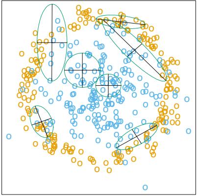
FIGURE 13.14. Neighborhoods found by the DANN procedure, at various query points (centers of the crosses). There are two classes in the data, with one class surrounding the other. 50 nearest-neighbors were used to estimate the local metrics. Shown are the resulting metrics used to form 15-nearest-neighborhoods.

in these cases the between matrix B = 0, and the Σ in (13.8) is the identity matrix.

13.4.1 Example

Here we generate two-class data in ten dimensions, analogous to the twodimensional example of Figure 13.14. All ten predictors in class 1 are independent standard normal, conditioned on the radius being greater than 22.4 and less than 40, while the predictors in class 2 are independent standard normal without the restriction. There are 250 observations in each class. Hence the first class almost completely surrounds the second class in the full ten-dimensional space.

In this example there are no pure noise variables, the kind that a nearestneighbor subset selection rule might be able to weed out. At any given point in the feature space, the class discrimination occurs along only one direction. However, this direction changes as we move across the feature space and all variables are important somewhere in the space.

Figure 13.15 shows boxplots of the test error rates over ten realizations, for standard 5-nearest-neighbors, LVQ, and discriminant adaptive 5-nearest-neighbors. We used 50 prototypes per class for LVQ, to make it comparable to 5 nearest-neighbors (since 250/5 = 50). The adaptive metric significantly reduces the error rate, compared to LVQ or standard nearest-neighbors.

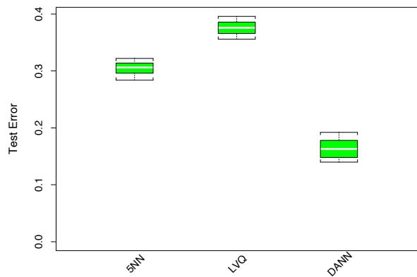
FIGURE 13.15. Ten-dimensional simulated example: boxplots of the test error rates over ten realizations, for standard 5-nearest-neighbors, LVQ with 50 centers, and discriminant-adaptive 5-nearest-neighbors

13.4.2 Global Dimension Reduction for Nearest-Neighbors

The discriminant-adaptive nearest-neighbor method carries out local dimension reduction—that is, dimension reduction separately at each query point. In many problems we can also benefit from global dimension reduction, that is, apply a nearest-neighbor rule in some optimally chosen subspace of the original feature space. For example, suppose that the two classes form two nested spheres in four dimensions of feature space, and there are an additional six noise features whose distribution is independent of class. Then we would like to discover the important four-dimensional subspace, and carry out nearest-neighbor classification in that reduced subspace. Hastie and Tibshirani (1996a) discuss a variation of the discriminantadaptive nearest-neighbor method for this purpose. At each training point xi, the between-centroids sum of squares matrix Bⁱ is computed, and then these matrices are averaged over all training points:

\[ \bar{\mathbf{B}} = \frac{1}{N} \sum\_{i=1}^{N} \mathbf{B}\_i. \tag{13.10} \]

Let e1, e2,…,e^p be the eigenvectors of the matrix B¯ , ordered from largest to smallest eigenvalue θk. Then these eigenvectors span the optimal subspaces for global subspace reduction. The derivation is based on the fact that the best rank-L approximation to B¯ , B¯ [L] = #^{L ℓ}=1 θℓeℓe^{T ℓ} , solves the least squares problem

\[\min\_{\text{rank}(\mathbf{M})=L} \sum\_{i=1}^{N} \text{trace}[(\mathbf{B}\_i - \mathbf{M})^2]. \tag{13.11}\]

Since each Bⁱ contains information on (a) the local discriminant subspace, and (b) the strength of discrimination in that subspace, (13.11) can be seen

480 13. Prototypes and Nearest-Neighbors

as a way of finding the best approximating subspace of dimension L to a series of N subspaces by weighted least squares (Exercise 13.5.)

In the four-dimensional sphere example mentioned above and examined in Hastie and Tibshirani (1996a), four of the eigenvalues θ^ℓ turn out to be large (having eigenvectors nearly spanning the interesting subspace), and the remaining six are near zero. Operationally, we project the data into the leading four-dimensional subspace, and then carry out nearest neighbor classification. In the satellite image classification example in Section 13.3.2, the technique labeled DANN in Figure 13.8 used 5-nearest-neighbors in a globally reduced subspace. There are also connections of this technique with the sliced inverse regression proposal of Duan and Li (1991). These authors use similar ideas in the regression setting, but do global rather than local computations. They assume and exploit spherical symmetry of the feature distribution to estimate interesting subspaces.

13.5 Computational Considerations

One drawback of nearest-neighbor rules in general is the computational load, both in finding the neighbors and storing the entire training set. With N observations and p predictors, nearest-neighbor classification requires N p operations to find the neighbors per query point. There are fast algorithms for finding nearest-neighbors (Friedman et al., 1975; Friedman et al., 1977) which can reduce this load somewhat. Hastie and Simard (1998) reduce the computations for tangent distance by developing analogs of K-means clustering in the context of this invariant metric.

Reducing the storage requirements is more difficult, and various editing and condensing procedures have been proposed. The idea is to isolate a subset of the training set that suffices for nearest-neighbor predictions, and throw away the remaining training data. Intuitively, it seems important to keep the training points that are near the decision boundaries and on the correct side of those boundaries, while some points far from the boundaries could be discarded.

The multi-edit algorithm of Devijver and Kittler (1982) divides the data cyclically into training and test sets, computing a nearest neighbor rule on the training set and deleting test points that are misclassified. The idea is to keep homogeneous clusters of training observations.

The condensing procedure of Hart (1968) goes further, trying to keep only important exterior points of these clusters. Starting with a single randomly chosen observation as the training set, each additional data item is processed one at a time, adding it to the training set only if it is misclassified by a nearest-neighbor rule computed on the current training set.

These procedures are surveyed in Dasarathy (1991) and Ripley (1996). They can also be applied to other learning procedures besides nearestneighbors. While such methods are sometimes useful, we have not had much practical experience with them, nor have we found any systematic comparison of their performance in the literature.

Bibliographic Notes

The nearest-neighbor method goes back at least to Fix and Hodges (1951). The extensive literature on the topic is reviewed by Dasarathy (1991); Chapter 6 of Ripley (1996) contains a good summary. K-means clustering is due to Lloyd (1957) and MacQueen (1967). Kohonen (1989) introduced learning vector quantization. The tangent distance method is due to Simard et al. (1993). Hastie and Tibshirani (1996a) proposed the discriminant adaptive nearest-neighbor technique.

Exercises

Ex. 13.1 Consider a Gaussian mixture model where the covariance matrices are assumed to be scalar: Σ^r = σI ∀r = 1,…,R, and σ is a fixed parameter. Discuss the analogy between the K-means clustering algorithm and the EM algorithm for fitting this mixture model in detail. Show that in the limit σ → 0 the two methods coincide.

Ex. 13.2 Derive formula (13.7) for the median radius of the 1-nearestneighborhood.

Ex. 13.3 Let E^∗ be the error rate of the Bayes rule in a K-class problem, where the true class probabilities are given by pk(x), k = 1,…,K. Assuming the test point and training point have identical features x, prove (13.5)

\[\sum\_{k=1}^{K} p\_k(x)(1 - p\_k(x)) \le 2(1 - p\_{k^\*}(x)) - \frac{K}{K - 1}(1 - p\_{k^\*}(x))^2.\]

where k^∗ = arg max^k pk(x). Hence argue that the error rate of the 1 nearest-neighbor rule converges in L1, as the size of the training set increases, to a value E1, bounded above by

\[E^\* \left( 2 - E^\* \frac{K}{K-1} \right). \tag{13.12}\]

[This statement of the theorem of Cover and Hart (1967) is taken from Chapter 6 of Ripley (1996), where a short proof is also given].

482 13. Prototypes and Nearest-Neighbors

Ex. 13.4 Consider an image to be a function ^F(x) : IR² 5→ IR¹ over the twodimensional spatial domain (paper coordinates). Then F(c+x0+A(x−x0)) represents an affine transformation of the image F, where A is a 2 × 2 matrix.

• 1. Decompose A (via Q-R) in such a way that parameters identifying the four affine transformations (two scale, shear and rotation) are clearly identified.
• 2. Using the chain rule, show that the derivative of F(c+x0+A(x−x0)) w.r.t. each of these parameters can be represented in terms of the two spatial derivatives of F.
• 3. Using a two-dimensional kernel smoother (Chapter 6), describe how to implement this procedure when the images are quantized to 16×16 pixels.

Ex. 13.5 Let Bi, i = 1, 2,…,N be square p × p positive semi-definite matrices and let B¯ = (1/N) #Bi. Write the eigen-decomposition of ^B¯ # as ^{p ℓ}=1 θℓeℓe^{T ℓ} with θ^ℓ ≥ θℓ−¹ ≥ ··· ≥ θ1. Show that the best rank-L approximation for the Bi,

\[\min\_{\text{rank}(\mathbf{M})=L} \sum\_{i=1}^{N} \text{trace}[(\mathbf{B}\_i - \mathbf{M})^2],\]

is given by B¯ [L] = #^{L ℓ}=1 θℓeℓe^{T ℓ} . (Hint: Write #^{N i}=1 trace[(B^{i − M})²] as

\[\sum\_{i=1}^{N} \text{trace}[(\mathbf{B}\_i - \bar{\mathbf{B}})^2] + \sum\_{i=1}^{N} \text{trace}[(\mathbf{M} - \bar{\mathbf{B}})^2]).\]

Ex. 13.6 Here we consider the problem of shape averaging. In particular, ^Li, i = 1,…,M are each ^{N ×} 2 matrices of points in IR², each sampled from corresponding positions of handwritten (cursive) letters. We seek an ^affine invariant average ^V, also ^{N ×} 2, ^{VT V = I}, of the ^M letters ^Li with the following property: V minimizes

\[\sum\_{j=1}^{M} \min\_{\mathbf{A}\_j} \left\| \mathbf{L}\_j - \mathbf{V} \mathbf{A}\_j \right\|^2.\]

Characterize the solution.

This solution can suffer if some of the letters are big and dominate the average. An alternative approach is to minimize instead:

\[\sum\_{j=1}^{M} \min\_{\mathbf{A}\_j} \left\| \mathbf{L}\_j \mathbf{A}\_j^\* - \mathbf{V} \right\|^2.\]

Derive the solution to this problem. How do the criteria differ? Use the SVD of the L^j to simplify the comparison of the two approaches.

Ex. 13.7 Consider the application of nearest-neighbors to the “easy” and “hard” problems in the left panel of Figure 13.5.

• 1. Replicate the results in the left panel of Figure 13.5.
• 2. Estimate the misclassification errors using fivefold cross-validation, and compare the error rate curves to those in 1.
• 3. Consider an “AIC-like” penalization of the training set misclassification error. Specifically, add 2t/N to the training set misclassification error, where t is the approximate number of parameters N/r, r being the number of nearest-neighbors. Compare plots of the resulting penalized misclassification error to those in 1 and 2. Which method gives a better estimate of the optimal number of nearest-neighbors: cross-validation or AIC?

Ex. 13.8 Generate data in two classes, with two features. These features are all independent Gaussian variates with standard deviation 1. Their mean vectors are (−1, −1) in class 1 and (1, 1) in class 2. To each feature vector apply a random rotation of angle θ, θ chosen uniformly from 0 to 2π. Generate 50 observations from each class to form the training set, and 500 in each class as the test set. Apply four different classifiers:

• 1. Nearest-neighbors.
• 2. Nearest-neighbors with hints: ten randomly rotated versions of each data point are added to the training set before applying nearestneighbors.
• 3. Invariant metric nearest-neighbors, using Euclidean distance invariant to rotations about the origin.
• 4. Tangent distance nearest-neighbors.

In each case choose the number of neighbors by tenfold cross-validation. Compare the results.

484 13. Prototypes and Nearest-Neighbors

This is page 485 Printer: Opaque this

14 Unsupervised Learning

14.1 Introduction

The previous chapters have been concerned with predicting the values of one or more outputs or response variables Y = (Y1,…,Ym) for a given set of input or predictor variables X^T = (X1,…,Xp). Denote by xT ⁱ = (xi1,…,xip) the inputs for the ith training case, and let yⁱ be a response measurement. The predictions are based on the training sample (x1, y1),…,(x^N , y^N ) of previously solved cases, where the joint values of all of the variables are known. This is called supervised learning or “learning with a teacher.” Under this metaphor the “student” presents an answer ˆyⁱ for each xⁱ in the training sample, and the supervisor or “teacher” provides either the correct answer and/or an error associated with the student’s answer. This is usually characterized by some loss function L(y, yˆ), for example, ^L(y, ^yˆ)=(^{y − y}ˆ)².

If one supposes that (X, Y ) are random variables represented by some joint probability density Pr(X, Y ), then supervised learning can be formally characterized as a density estimation problem where one is concerned with determining properties of the conditional density Pr(Y |X). Usually the properties of interest are the “location” parameters µ that minimize the expected error at each x,

\[\mu(x) = \operatorname\*{argmin}\_{\theta} E\_{Y|X} L(Y, \theta). \tag{14.1}\]

486 14. Unsupervised Learning

Conditioning one has

\[\Pr(X, Y) = \Pr(Y|X) \cdot \Pr(X),\]

where Pr(X) is the joint marginal density of the X values alone. In supervised learning Pr(X) is typically of no direct concern. One is interested mainly in the properties of the conditional density Pr(Y |X). Since Y is often of low dimension (usually one), and only its location µ(x) is of interest, the problem is greatly simplified. As discussed in the previous chapters, there are many approaches for successfully addressing supervised learning in a variety of contexts.

In this chapter we address unsupervised learning or “learning without a teacher.” In this case one has a set of N observations (x1, x2,…,x^N ) of a random p-vector X having joint density Pr(X). The goal is to directly infer the properties of this probability density without the help of a supervisor or teacher providing correct answers or degree-of-error for each observation. The dimension of X is sometimes much higher than in supervised learning, and the properties of interest are often more complicated than simple location estimates. These factors are somewhat mitigated by the fact that X represents all of the variables under consideration; one is not required to infer how the properties of Pr(X) change, conditioned on the changing values of another set of variables.

In low-dimensional problems (say p ≤ 3), there are a variety of effective nonparametric methods for directly estimating the density Pr(X) itself at all X-values, and representing it graphically (Silverman, 1986, e.g.). Owing to the curse of dimensionality, these methods fail in high dimensions. One must settle for estimating rather crude global models, such as Gaussian mixtures or various simple descriptive statistics that characterize Pr(X).

Generally, these descriptive statistics attempt to characterize X-values, or collections of such values, where Pr(X) is relatively large. Principal components, multidimensional scaling, self-organizing maps, and principal curves, for example, attempt to identify low-dimensional manifolds within the X-space that represent high data density. This provides information about the associations among the variables and whether or not they can be considered as functions of a smaller set of “latent” variables. Cluster analysis attempts to find multiple convex regions of the X-space that contain modes of Pr(X). This can tell whether or not Pr(X) can be represented by a mixture of simpler densities representing distinct types or classes of observations. Mixture modeling has a similar goal. Association rules attempt to construct simple descriptions (conjunctive rules) that describe regions of high density in the special case of very high dimensional binary-valued data.

With supervised learning there is a clear measure of success, or lack thereof, that can be used to judge adequacy in particular situations and to compare the effectiveness of different methods over various situations. Lack of success is directly measured by expected loss over the joint distribution Pr(X, Y ). This can be estimated in a variety of ways including cross-validation. In the context of unsupervised learning, there is no such direct measure of success. It is difficult to ascertain the validity of inferences drawn from the output of most unsupervised learning algorithms. One must resort to heuristic arguments not only for motivating the algorithms, as is often the case in supervised learning as well, but also for judgments as to the quality of the results. This uncomfortable situation has led to heavy proliferation of proposed methods, since effectiveness is a matter of opinion and cannot be verified directly.

In this chapter we present those unsupervised learning techniques that are among the most commonly used in practice, and additionally, a few others that are favored by the authors.

14.2 Association Rules

Association rule analysis has emerged as a popular tool for mining commercial data bases. The goal is to find joint values of the variables X = (X1, X2,…,Xp) that appear most frequently in the data base. It is most often applied to binary-valued data X^j ∈ {0, 1}, where it is referred to as “market basket” analysis. In this context the observations are sales transactions, such as those occurring at the checkout counter of a store. The variables represent all of the items sold in the store. For observation i, each variable X^j is assigned one of two values; xij = 1 if the jth item is purchased as part of the transaction, whereas xij = 0 if it was not purchased. Those variables that frequently have joint values of one represent items that are frequently purchased together. This information can be quite useful for stocking shelves, cross-marketing in sales promotions, catalog design, and consumer segmentation based on buying patterns.

More generally, the basic goal of association rule analysis is to find a collection of prototype X-values v1,…,v^L for the feature vector X, such that the probability density Pr(vl) evaluated at each of those values is relatively large. In this general framework, the problem can be viewed as “mode finding” or “bump hunting.” As formulated, this problem is impossibly difficult. A natural estimator for each Pr(vl) is the fraction of observations for which X = vl. For problems that involve more than a small number of variables, each of which can assume more than a small number of values, the number of observations for which X = v^l will nearly always be too small for reliable estimation. In order to have a tractable problem, both the goals of the analysis and the generality of the data to which it is applied must be greatly simplified.

The first simplification modifies the goal. Instead of seeking values x where Pr(x) is large, one seeks regions of the X-space with high probability

488 14. Unsupervised Learning

content relative to their size or support. Let S^j represent the set of all possible values of the jth variable (its support), and let s^j ⊆ S^j be a subset of these values. The modified goal can be stated as attempting to find subsets of variable values s1,…,s^p such that the probability of each of the variables simultaneously assuming a value within its respective subset,

\[\Pr\left[\bigcap\_{j=1}^{p} (X\_j \in s\_j)\right],\tag{14.2}\]

is relatively large. The intersection of subsets ^{∩p j}=1(X^j ∈ s^j ) is called a conjunctive rule. For quantitative variables the subsets s^j are contiguous intervals; for categorical variables the subsets are delineated explicitly. Note that if the subset s^j is in fact the entire set of values s^j = S^j , as is often the case, the variable X^j is said not to appear in the rule (14.2).

14.2.1 Market Basket Analysis

General approaches to solving (14.2) are discussed in Section 14.2.5. These can be quite useful in many applications. However, they are not feasible for the very large (^{p ≈ 104}, ^{N ≈ 108}) commercial data bases to which market basket analysis is often applied. Several further simplifications of (14.2) are required. First, only two types of subsets are considered; either s^j consists of a single value of X^j , s^j = v0^j , or it consists of the entire set of values that X^j can assume, s^j = S^j . This simplifies the problem (14.2) to finding subsets of the integers J ⊂ {1,…,p}, and corresponding values v0^j , j ∈ J , such that

\[\Pr\left[\bigcap\_{j\in\mathcal{J}} (X\_j = v\_{0j})\right] \tag{14.3}\]

is large. Figure 14.1 illustrates this assumption.

One can apply the technique of dummy variables to turn (14.3) into a problem involving only binary-valued variables. Here we assume that the support S^j is finite for each variable X^j . Specifically, a new set of variables Z1,…,Z^K is created, one such variable for each of the values vlj attainable by each of the original variables X1,…,Xp. The number of dummy variables K is

\[K = \sum\_{j=1}^{p} |\mathcal{S}\_j|,\]

where |S^j | is the number of distinct values attainable by X^j . Each dummy variable is assigned the value Z^k = 1 if the variable with which it is associated takes on the corresponding value to which Z^k is assigned, and Z^k = 0 otherwise. This transforms (14.3) to finding a subset of the integers K ⊂ {1,…,K} such that

FIGURE 14.1. Simplifications for association rules. Here there are two inputs X¹ and X2, taking four and six distinct values, respectively. The red squares indicate areas of high density. To simplify the computations, we assume that the derived subset corresponds to either a single value of an input or all values. With this assumption we could find either the middle or right pattern, but not the left one.

\[\Pr\left[\bigcap\_{k\in\mathcal{K}} (Z\_k = 1)\right] = \Pr\left[\prod\_{k\in\mathcal{K}} Z\_k = 1\right] \tag{14.4}\]

is large. This is the standard formulation of the market basket problem. The set K is called an “item set.” The number of variables Z^k in the item set is called its “size” (note that the size is no bigger than p). The estimated value of (14.4) is taken to be the fraction of observations in the data base for which the conjunction in (14.4) is true:

\[\widehat{\mathrm{Pr}}\left[\prod\_{k\in\mathcal{K}}(Z\_k=1)\right] = \frac{1}{N}\sum\_{i=1}^{N}\prod\_{k\in\mathcal{K}}z\_{ik}.\tag{14.5}\]

Here zik is the value of Z^k for this ith case. This is called the “support” or “prevalence” ^T(K) of the item set ^K. An observation ⁱ for which ^{K k}∈^K zik = 1 is said to “contain” the item set K.

In association rule mining a lower support bound t is specified, and one seeks all item sets K^l that can be formed from the variables Z1,…,Z^K with support in the data base greater than this lower bound t

\[\{\mathcal{K}\_l | T(\mathcal{K}\_l) > t\}.\tag{14.6}\]

14.2.2 The Apriori Algorithm

The solution to this problem (14.6) can be obtained with feasible computation for very large data bases provided the threshold t is adjusted so that (14.6) consists of only a small fraction of all 2^K possible item sets. The “Apriori” algorithm (Agrawal et al., 1995) exploits several aspects of the

490 14. Unsupervised Learning

curse of dimensionality to solve (14.6) with a small number of passes over the data. Specifically, for a given support threshold t:

• The cardinality |{K| T(K) > t}| is relatively small.
• Any item set L consisting of a subset of the items in K must have support greater than or equal to that of K, L ⊆ K ⇒ T(L) ≥ T(K).

The first pass over the data computes the support of all single-item sets. Those whose support is less than the threshold are discarded. The second pass computes the support of all item sets of size two that can be formed from pairs of the single items surviving the first pass. In other words, to generate all frequent itemsets with |K| = m, we need to consider only candidates such that all of their m ancestral item sets of size m − 1 are frequent. Those size-two item sets with support less than the threshold are discarded. Each successive pass over the data considers only those item sets that can be formed by combining those that survived the previous pass with those retained from the first pass. Passes over the data continue until all candidate rules from the previous pass have support less than the specified threshold. The Apriori algorithm requires only one pass over the data for each value of |K|, which is crucial since we assume the data cannot be fitted into a computer’s main memory. If the data are sufficiently sparse (or if the threshold t is high enough), then the process will terminate in reasonable time even for huge data sets.

There are many additional tricks that can be used as part of this strategy to increase speed and convergence (Agrawal et al., 1995). The Apriori algorithm represents one of the major advances in data mining technology.

Each high support item set K (14.6) returned by the Apriori algorithm is cast into a set of “association rules.” The items Zk, k ∈ K, are partitioned into two disjoint subsets, A ∪ B = K, and written

\[A \Rightarrow B.\tag{14.7}\]

The first item subset A is called the “antecedent” and the second B the “consequent.” Association rules are defined to have several properties based on the prevalence of the antecedent and consequent item sets in the data base. The “support” of the rule T(A ⇒ B) is the fraction of observations in the union of the antecedent and consequent, which is just the support of the item set K from which they were derived. It can be viewed as an estimate (14.5) of the probability of simultaneously observing both item sets Pr(A and B) in a randomly selected market basket. The “confidence” or “predictability” C(A ⇒ B) of the rule is its support divided by the support of the antecedent

\[C(A \Rightarrow B) = \frac{T(A \Rightarrow B)}{T(A)},\tag{14.8}\]

which can be viewed as an estimate of Pr(B | A). The notation Pr(A), the probability of an item set A occurring in a basket, is an abbreviation for Pr(K ^k∈^A Z^k = 1). The “expected confidence” is defined as the support of the consequent T(B), which is an estimate of the unconditional probability Pr(B). Finally, the “lift” of the rule is defined as the confidence divided by the expected confidence

\[L(A \Rightarrow B) = \frac{C(A \Rightarrow B)}{T(B)}.\]

This is an estimate of the association measure Pr(A and B)/Pr(A)Pr(B).

As an example, suppose the item set K = {peanut butter, jelly, bread} and consider the rule {peanut butter, jelly} ⇒ {bread}. A support value of 0.03 for this rule means that peanut butter, jelly, and bread appeared together in 3% of the market baskets. A confidence of 0.82 for this rule implies that when peanut butter and jelly were purchased, 82% of the time bread was also purchased. If bread appeared in 43% of all market baskets then the rule {peanut butter, jelly} ⇒ {bread} would have a lift of 1.95.

The goal of this analysis is to produce association rules (14.7) with both high values of support and confidence (14.8). The Apriori algorithm returns all item sets with high support as defined by the support threshold t (14.6). A confidence threshold c is set, and all rules that can be formed from those item sets (14.6) with confidence greater than this value

\[\{A \Rightarrow B \mid C(A \Rightarrow B) > c\}\tag{14.9}\]

are reported. For each item set ^K of size |K| there are 2|K|−^{1 −} 1 rules of the form A ⇒ (K − A), A ⊂ K. Agrawal et al. (1995) present a variant of the Apriori algorithm that can rapidly determine which rules survive the confidence threshold (14.9) from all possible rules that can be formed from the solution item sets (14.6).

The output of the entire analysis is a collection of association rules (14.7) that satisfy the constraints

\[T(A \Rightarrow B) > t \quad \text{and} \quad C(A \Rightarrow B) > c.\]

These are generally stored in a data base that can be queried by the user. Typical requests might be to display the rules in sorted order of confidence, lift or support. More specifically, one might request such a list conditioned on particular items in the antecedent or especially the consequent. For example, a request might be the following:

Display all transactions in which ice skates are the consequent that have confidence over 80% and support of more than 2%.

This could provide information on those items (antecedent) that predicate sales of ice skates. Focusing on a particular consequent casts the problem into the framework of supervised learning.

Association rules have become a popular tool for analyzing very large commercial data bases in settings where market basket is relevant. That is

492 14. Unsupervised Learning

when the data can be cast in the form of a multidimensional contingency table. The output is in the form of conjunctive rules (14.4) that are easily understood and interpreted. The Apriori algorithm allows this analysis to be applied to huge data bases, much larger that are amenable to other types of analyses. Association rules are among data mining’s biggest successes.

Besides the restrictive form of the data to which they can be applied, association rules have other limitations. Critical to computational feasibility is the support threshold (14.6). The number of solution item sets, their size, and the number of passes required over the data can grow exponentially with decreasing size of this lower bound. Thus, rules with high confidence or lift, but low support, will not be discovered. For example, a high confidence rule such as vodka ⇒ caviar will not be uncovered owing to the low sales volume of the consequent caviar.

14.2.3 Example: Market Basket Analysis

We illustrate the use of Apriori on a moderately sized demographics data base. This data set consists of N = 9409 questionnaires filled out by shopping mall customers in the San Francisco Bay Area (Impact Resources, Inc., Columbus OH, 1987). Here we use answers to the first 14 questions, relating to demographics, for illustration. These questions are listed in Table 14.1. The data are seen to consist of a mixture of ordinal and (unordered) categorical variables, many of the latter having more than a few values. There are many missing values.

We used a freeware implementation of the Apriori algorithm due to Christian Borgelt¹. After removing observations with missing values, each ordinal predictor was cut at its median and coded by two dummy variables; each categorical predictor with k categories was coded by k dummy variables. This resulted in a 6876 × 50 matrix of 6876 observations on 50 dummy variables.

The algorithm found a total of 6288 association rules, involving ≤ 5 predictors, with support of at least 10%. Understanding this large set of rules is itself a challenging data analysis task. We will not attempt this here, but only illustrate in Figure 14.2 the relative frequency of each dummy variable in the data (top) and the association rules (bottom). Prevalent categories tend to appear more often in the rules, for example, the first category in language (English). However, others such as occupation are under-represented, with the exception of the first and fifth level.

Here are three examples of association rules found by the Apriori algorithm:

Association rule 1: Support 25%, confidence 99.7% and lift 1.03.

¹See http://fuzzy.cs.uni-magdeburg.de/∼borgelt.

FIGURE 14.2. Market basket analysis: relative frequency of each dummy variable (coding an input category) in the data (top), and the association rules found by the Apriori algorithm (bottom).

Feature	Demographic	# Values	Type
1	Sex	2	Categorical
2	Marital status	5	Categorical
3	Age	7	Ordinal
4	Education	6	Ordinal
5	Occupation	9	Categorical
6	Income	9	Ordinal
7	Years in Bay Area	5	Ordinal
8	Dual incomes	3	Categorical
9	Number in household	9	Ordinal
10	Number of children	9	Ordinal
11	Householder status	3	Categorical
12	Type of home	5	Categorical
13	Ethnic classification	8	Categorical
14	Language in home	3	Categorical

TABLE 14.1. Inputs for the demographic data.

, number in household = 1 number of children = 0 - ⇓ language in home = English

Association rule 2: Support 13.4%, confidence 80.8%, and lift 2.13.

\[ \begin{bmatrix} \text{langugage in home} & = &English \\ \text{householder status} & = & own \\ \text{occupation} & = & \{profission/managerial\} \\ & & \Downarrow \\ & & \text{income} \ge \\$40,000 \end{bmatrix} \]

Association rule 3: Support 26.5%, confidence 82.8% and lift 2.15.

⎡ ⎢ ⎢ ⎣ language in home = English income < $40,000 marital status = not married number of children = 0 ⎤ ⎥ ⎥ ⎦ ⇓

education ∈/ {college graduate, graduate study}

We chose the first and third rules based on their high support. The second rule is an association rule with a high-income consequent, and could be used to try to target high-income individuals.

As stated above, we created dummy variables for each category of the input predictors, for example, Z¹ = I(income < $40, 000) and Z² = I(income ≥ $40, 000) for below and above the median income. If we were interested only in finding associations with the high-income category, we would include Z² but not Z1. This is often the case in actual market basket problems, where we are interested in finding associations with the presence of a relatively rare item, but not associations with its absence.

14.2.4 Unsupervised as Supervised Learning

Here we discuss a technique for transforming the density estimation problem into one of supervised function approximation. This forms the basis for the generalized association rules described in the next section.

Let g(x) be the unknown data probability density to be estimated, and g0(x) be a specified probability density function used for reference. For example, g0(x) might be the uniform density over the range of the variables. Other possibilities are discussed below. The data set x1, x2,…,x^N is presumed to be an i.i.d. random sample drawn from g(x). A sample of size N⁰ can be drawn from g0(x) using Monte Carlo methods. Pooling these two data sets, and assigning mass w = N0/(N + N0) to those drawn from g(x), and w⁰ = N/(N + N0) to those drawn from g0(x), results in a random sample drawn from the mixture density (g(x) + g0(x)) /2. If one assigns the value Y = 1 to each sample point drawn from g(x) and Y = 0 those drawn from g0(x), then

\[\begin{aligned} \mu(x) &= E(Y \mid x) &= \frac{g(x)}{g(x) + g\_0(x)} \\ &= \frac{g(x)/g\_0(x)}{1 + g(x)/g\_0(x)} \end{aligned} \tag{14.10}\]

can be estimated by supervised learning using the combined sample

\[((y\_1, x\_1), (y\_2, x\_2), \dots, (y\_{N+N\_0}, x\_{N+N\_0})\tag{14.11}\]

as training data. The resulting estimate ˆµ(x) can be inverted to provide an estimate for g(x)

\[ \hat{g}(x) = g\_0(x) \frac{\hat{\mu}(x)}{1 - \hat{\mu}(x)}.\tag{14.12} \]

Generalized versions of logistic regression (Section 4.4) are especially well suited for this application since the log-odds,

\[f(x) = \log \frac{g(x)}{g\_0(x)},\tag{14.13}\]

are estimated directly. In this case one has

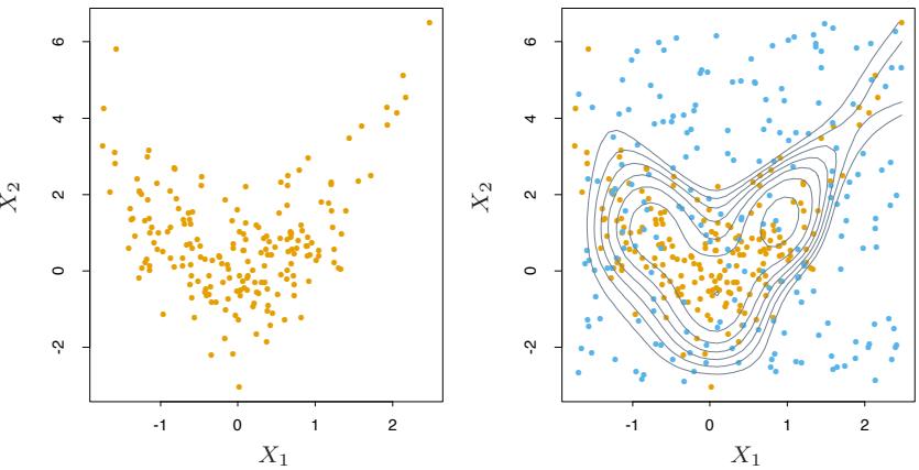
FIGURE 14.3. Density estimation via classification. (Left panel:) Training set of 200 data points. (Right panel:) Training set plus 200 reference data points, generated uniformly over the rectangle containing the training data. The training sample was labeled as class 1, and the reference sample class 0, and a semiparametric logistic regression model was fit to the data. Some contours for gˆ(x) are shown.

\[ \hat{g}(x) = g\_0(x) \, e^{\hat{f}(x)}.\tag{14.14} \]

An example is shown in Figure 14.3. We generated a training set of size 200 shown in the left panel. The right panel shows the reference data (blue) generated uniformly over the rectangle containing the training data. The training sample was labeled as class 1, and the reference sample class 0, and a logistic regression model, using a tensor product of natural splines (Section 5.2.1), was fit to the data. Some probability contours of ˆµ(x) are shown in the right panel; these are also the contours of the density estimate gˆ(x), since ˆg(x)=ˆµ(x)/(1 − µˆ(x)), is a monotone function. The contours roughly capture the data density.

In principle any reference density can be used for g0(x) in (14.14). In practice the accuracy of the estimate ˆg(x) can depend greatly on particular choices. Good choices will depend on the data density g(x) and the procedure used to estimate (14.10) or (14.13). If accuracy is the goal, g0(x) should be chosen so that the resulting functions µ(x) or f(x) are approximated easily by the method being used. However, accuracy is not always the primary goal. Both µ(x) and f(x) are monotonic functions of the density ratio g(x)/g0(x). They can thus be viewed as “contrast” statistics that provide information concerning departures of the data density g(x) from the chosen reference density g0(x). Therefore, in data analytic settings, a choice for g0(x) is dictated by types of departures that are deemed most interesting in the context of the specific problem at hand. For example, if departures from uniformity are of interest, g0(x) might be the a uniform density over the range of the variables. If departures from joint normality are of interest, a good choice for g0(x) would be a Gaussian distribution with the same mean vector and covariance matrix as the data. Departures from independence could be investigated by using

\[g\_0(x) = \prod\_{j=1}^p g\_j(x\_j),\tag{14.15}\]

where g^j (x^j ) is the marginal data density of X^j , the jth coordinate of X. A sample from this independent density (14.15) is easily generated from the data itself by applying a different random permutation to the data values of each of the variables.

As discussed above, unsupervised learning is concerned with revealing properties of the data density g(x). Each technique focuses on a particular property or set of properties. Although this approach of transforming the problem to one of supervised learning (14.10)–(14.14) seems to have been part of the statistics folklore for some time, it does not appear to have had much impact despite its potential to bring well-developed supervised learning methodology to bear on unsupervised learning problems. One reason may be that the problem must be enlarged with a simulated data set generated by Monte Carlo techniques. Since the size of this data set should be at least as large as the data sample N⁰ ≥ N, the computation and memory requirements of the estimation procedure are at least doubled. Also, substantial computation may be required to generate the Monte Carlo sample itself. Although perhaps a deterrent in the past, these increased computational requirements are becoming much less of a burden as increased resources become routinely available. We illustrate the use of supervising learning methods for unsupervised learning in the next section.

14.2.5 Generalized Association Rules

The more general problem (14.2) of finding high-density regions in the data space can be addressed using the supervised learning approach described above. Although not applicable to the huge data bases for which market basket analysis is feasible, useful information can be obtained from moderately sized data sets. The problem (14.2) can be formulated as finding subsets of the integers J ⊂ {1, 2,…,p} and corresponding value subsets s^j , j ∈ J for the corresponding variables X^j , such that

\[\widehat{\Pr}\left(\bigcap\_{j\in\mathcal{J}}(X\_j\in s\_j)\right) = \frac{1}{N}\sum\_{i=1}^N I\left(\bigcap\_{j\in\mathcal{J}}(x\_{ij}\in s\_j)\right) \tag{14.16}\]

is large. Following the nomenclature of association rule analysis, {(X^j ∈ s^j )}j∈^J will be called a “generalized” item set. The subsets s^j corresponding to quantitative variables are taken to be contiguous intervals within

498 14. Unsupervised Learning

their range of values, and subsets for categorical variables can involve more than a single value. The ambitious nature of this formulation precludes a thorough search for all generalized item sets with support (14.16) greater than a specified minimum threshold, as was possible in the more restrictive setting of market basket analysis. Heuristic search methods must be employed, and the most one can hope for is to find a useful collection of such generalized item sets.

Both market basket analysis (14.5) and the generalized formulation (14.16) implicitly reference the uniform probability distribution. One seeks item sets that are more frequent than would be expected if all joint data values (x1, x2,…,x^N ) were uniformly distributed. This favors the discovery of item sets whose marginal constituents (X^j ∈ s^j ) are individually frequent, that is, the quantity

\[\frac{1}{N} \sum\_{i=1}^{N} I(x\_{ij} \in s\_j) \tag{14.17}\]

is large. Conjunctions of frequent subsets (14.17) will tend to appear more often among item sets of high support (14.16) than conjunctions of marginally less frequent subsets. This is why the rule vodka ⇒ caviar is not likely to be discovered in spite of a high association (lift); neither item has high marginal support, so that their joint support is especially small. Reference to the uniform distribution can cause highly frequent item sets with low associations among their constituents to dominate the collection of highest support item sets.

Highly frequent subsets s^j are formed as disjunctions of the most frequent X^j -values. Using the product of the variable marginal data densities (14.15) as a reference distribution removes the preference for highly frequent values of the individual variables in the discovered item sets. This is because the density ratio g(x)/g0(x) is uniform if there are no associations among the variables (complete independence), regardless of the frequency distribution of the individual variable values. Rules like vodka ⇒ caviar would have a chance to emerge. It is not clear however, how to incorporate reference distributions other than the uniform into the Apriori algorithm. As explained in Section 14.2.4, it is straightforward to generate a sample from the product density (14.15), given the original data set.

After choosing a reference distribution, and drawing a sample from it as in (14.11), one has a supervised learning problem with a binary-valued output variable Y ∈ {0, 1}. The goal is to use this training data to find regions

\[R = \bigcap\_{j \in \mathcal{J}} (X\_j \in s\_j) \tag{14.18}\]

for which the target function µ(x) = E(Y | x) is relatively large. In addition, one might wish to require that the data support of these regions

14.2 Association Rules 499

\[T(R) = \int\_{x \in R} g(x) \, dx \tag{14.19}\]

not be too small.

14.2.6 Choice of Supervised Learning Method

The regions (14.18) are defined by conjunctive rules. Hence supervised methods that learn such rules would be most appropriate in this context. The terminal nodes of a CART decision tree are defined by rules precisely of the form (14.18). Applying CART to the pooled data (14.11) will produce a decision tree that attempts to model the target (14.10) over the entire data space by a disjoint set of regions (terminal nodes). Each region is defined by a rule of the form (14.18). Those terminal nodes t with high average y-values

\[ \bar{y}\_t = \text{ave}(y\_i \mid x\_i \in t), \]

are candidates for high-support generalized item sets (14.16). The actual (data) support is given by

\[T(R) = \bar{y}\_t \cdot \frac{N\_t}{N + N\_0},\]

where N^t is the number of (pooled) observations within the region represented by the terminal node. By examining the resulting decision tree, one might discover interesting generalized item sets of relatively high-support. These can then be partitioned into antecedents and consequents in a search for generalized association rules of high confidence and/or lift.

Another natural learning method for this purpose is the patient rule induction method PRIM described in Section 9.3. PRIM also produces rules precisely of the form (14.18), but it is especially designed for finding high-support regions that maximize the average target (14.10) value within them, rather than trying to model the target function over the entire data space. It also provides more control over the support/average-target-value tradeoff.

Exercise 14.3 addresses an issue that arises with either of these methods when we generate random data from the product of the marginal distributions.

14.2.7 Example: Market Basket Analysis (Continued)

We illustrate the use of PRIM on the demographics data of Table 14.1.

Three of the high-support generalized item sets emerging from the PRIM analysis were the following:

Item set 1: Support= 24%.

500 14. Unsupervised Learning

⎡ ⎣

marital status = married householder status = own type of home ̸= apartment ⎤ ⎦

Item set 2: Support= 24%.

⎡ ⎢ ⎢ ⎣ age ≤ 24 marital status ∈ {living together-not married, single} occupation ∈/ {professional, homemaker, retired} householder status ∈ {rent, live with family}

⎤ ⎥ ⎥ ⎦

⎤ ⎥ ⎥ ⎥ ⎥ ⎥ ⎥ ⎦

Item set 3: Support= 15%.

⎡	householder status	=	rent
⎢	type of home	̸=	house
⎢ ⎢	number in household	≤	2
⎢ ⎢	number of children	=	0
⎢ ⎣	occupation	∈/	{homemaker, student, unemployed}
	income	∈	[$20,000, $150,000]

Generalized association rules derived from these item sets with confidence (14.8) greater than 95% are the following:

Association rule 1: Support 25%, confidence 99.7% and lift 1.35.

, marital status = married householder status = own - ⇓ type of home ̸= apartment

Association rule 2: Support 25%, confidence 98.7% and lift 1.97.

⎡ ⎣ age ≤ 24 occupation ∈/ {professional, homemaker, retired} householder status ∈ {rent, live with family} ⎤ ⎦ ⇓

marital status ∈ {single, living together-not married}

Association rule 3: Support 25%, confidence 95.9% and lift 2.61.

, householder status = own type of home ̸⁼ apartment - ⇓ marital status = married

⎤ ⎥ ⎥ ⎥ ⎥ ⎦

Association rule 4: Support 15%, confidence 95.4% and lift 1.50.

⎡ ⎢ ⎢ ⎢ ⎢ ⎣ householder status = rent type of home ̸= house number in household ≤ 2 occupation ∈/ {homemaker, student, unemployed} income ∈ [$20,000, $150,000] ⇓

number of children = 0

There are no great surprises among these particular rules. For the most part they verify intuition. In other contexts where there is less prior information available, unexpected results have a greater chance to emerge. These results do illustrate the type of information generalized association rules can provide, and that the supervised learning approach, coupled with a ruled induction method such as CART or PRIM, can uncover item sets exhibiting high associations among their constituents.

How do these generalized association rules compare to those found earlier by the Apriori algorithm? Since the Apriori procedure gives thousands of rules, it is difficult to compare them. However some general points can be made. The Apriori algorithm is exhaustive—it finds all rules with support greater than a specified amount. In contrast, PRIM is a greedy algorithm and is not guaranteed to give an “optimal” set of rules. On the other hand, the Apriori algorithm can deal only with dummy variables and hence could not find some of the above rules. For example, since type of home is a categorical input, with a dummy variable for each level, Apriori could not find a rule involving the set

type of home ̸= apartment.

To find this set, we would have to code a dummy variable for apartment versus the other categories of type of home. It will not generally be feasible to precode all such potentially interesting comparisons.

14.3 Cluster Analysis

Cluster analysis, also called data segmentation, has a variety of goals. All relate to grouping or segmenting a collection of objects into subsets or “clusters,” such that those within each cluster are more closely related to one another than objects assigned to different clusters. An object can be described by a set of measurements, or by its relation to other objects. In addition, the goal is sometimes to arrange the clusters into a natural hierarchy. This involves successively grouping the clusters themselves so

FIGURE 14.4. Simulated data in the plane, clustered into three classes (represented by orange, blue and green) by the K-means clustering algorithm

that at each level of the hierarchy, clusters within the same group are more similar to each other than those in different groups.

Cluster analysis is also used to form descriptive statistics to ascertain whether or not the data consists of a set distinct subgroups, each group representing objects with substantially different properties. This latter goal requires an assessment of the degree of difference between the objects assigned to the respective clusters.

Central to all of the goals of cluster analysis is the notion of the degree of similarity (or dissimilarity) between the individual objects being clustered. A clustering method attempts to group the objects based on the definition of similarity supplied to it. This can only come from subject matter considerations. The situation is somewhat similar to the specification of a loss or cost function in prediction problems (supervised learning). There the cost associated with an inaccurate prediction depends on considerations outside the data.

Figure 14.4 shows some simulated data clustered into three groups via the popular K-means algorithm. In this case two of the clusters are not well separated, so that “segmentation” more accurately describes the part of this process than “clustering.” K-means clustering starts with guesses for the three cluster centers. Then it alternates the following steps until convergence:

• for each data point, the closest cluster center (in Euclidean distance) is identified;

• each cluster center is replaced by the coordinate-wise average of all data points that are closest to it.

We describe K-means clustering in more detail later, including the problem of how to choose the number of clusters (three in this example). Kmeans clustering is a top-down procedure, while other cluster approaches that we discuss are bottom-up. Fundamental to all clustering techniques is the choice of distance or dissimilarity measure between two objects. We first discuss distance measures before describing a variety of algorithms for clustering.

14.3.1 Proximity Matrices

Sometimes the data is represented directly in terms of the proximity (alikeness or affinity) between pairs of objects. These can be either similarities or dissimilarities (difference or lack of affinity). For example, in social science experiments, participants are asked to judge by how much certain objects differ from one another. Dissimilarities can then be computed by averaging over the collection of such judgments. This type of data can be represented by an N ×N matrix D, where N is the number of objects, and each element dii′ records the proximity between the ith and i ′ th objects. This matrix is then provided as input to the clustering algorithm.

Most algorithms presume a matrix of dissimilarities with nonnegative entries and zero diagonal elements: dii = 0, i = 1, 2,…,N. If the original data were collected as similarities, a suitable monotone-decreasing function can be used to convert them to dissimilarities. Also, most algorithms assume symmetric dissimilarity matrices, so if the original matrix D is not symmetric it must be replaced by (D+D^T )/2. Subjectively judged dissimilarities are seldom distances in the strict sense, since the triangle inequality dii′ ≤ dik+di′k, for all k ∈ {1,…,N} does not hold. Thus, some algorithms that assume distances cannot be used with such data.

14.3.2 Dissimilarities Based on Attributes

Most often we have measurements xij for i = 1, 2,…,N, on variables j = 1, 2,…,p (also called attributes). Since most of the popular clustering algorithms take a dissimilarity matrix as their input, we must first construct pairwise dissimilarities between the observations. In the most common case, we define a dissimilarity d^j (xij , xi′^j ) between values of the jth attribute, and then define

\[D(x\_i, x\_{i'}) = \sum\_{j=1}^{p} d\_j(x\_{ij}, x\_{i'j}) \tag{14.20}\]

as the dissimilarity between objects i and i ′ . By far the most common choice is squared distance

504 14. Unsupervised Learning

\[d\_j(x\_{ij}, x\_{i'j}) = (x\_{ij} - x\_{i'j})^2. \tag{14.21}\]

However, other choices are possible, and can lead to potentially different results. For nonquantitative attributes (e.g., categorical data), squared distance may not be appropriate. In addition, it is sometimes desirable to weigh attributes differently rather than giving them equal weight as in (14.20).

We first discuss alternatives in terms of the attribute type:

Quantitative variables. Measurements of this type of variable or attribute are represented by continuous real-valued numbers. It is natural to define the “error” between them as a monotone-increasing function of their absolute difference

\[d(x\_i, x\_{i'}) = l(|x\_i - x\_{i'}|).\]

Besides squared-error loss (x^{i −}xi′ )², a common choice is the identity (absolute error). The former places more emphasis on larger differences than smaller ones. Alternatively, clustering can be based on the correlation

\[\rho(x\_i, x\_{i'}) = \frac{\sum\_j (x\_{ij} - \bar{x}\_i)(x\_{i'j} - \bar{x}\_{i'})}{\sqrt{\sum\_j (x\_{ij} - \bar{x}\_i)^2 \sum\_j (x\_{i'j} - \bar{x}\_{i'})^2}},\tag{14.22}\]

with ¯xⁱ = # ^j xij/p. Note that this is averaged over variables, not observations. If the observations are first standardized, then # ^j (xij − ^xi′^j )^{2 ∝} 2(1−ρ(xi, xi′ )). Hence clustering based on correlation (similarity) is equivalent to that based on squared distance (dissimilarity).

Ordinal variables. The values of this type of variable are often represented as contiguous integers, and the realizable values are considered to be an ordered set. Examples are academic grades (A, B, C, D, F), degree of preference (can’t stand, dislike, OK, like, terrific). Rank data are a special kind of ordinal data. Error measures for ordinal variables are generally defined by replacing their M original values with

\[\frac{i - 1/2}{M}, \ i = 1, \ldots, M \tag{14.23}\]

in the prescribed order of their original values. They are then treated as quantitative variables on this scale.

Categorical variables. With unordered categorical (also called nominal) variables, the degree-of-difference between pairs of values must be delineated explicitly. If the variable assumes M distinct values, these can be arranged in a symmetric M ×M matrix with elements Lrr′ = Lr′r, Lrr = 0, Lrr′ ≥ 0. The most common choice is Lrr′ = 1 for all ^r ̸^{= r}′ , while unequal losses can be used to emphasize some errors more than others.

14.3.3 Object Dissimilarity

Next we define a procedure for combining the p-individual attribute dissimilarities d^j (xij , xi′^j ), j = 1, 2,…,p into a single overall measure of dissimilarity D(xi, xi′ ) between two objects or observations (xi, xi′ ) possessing the respective attribute values. This is nearly always done by means of a weighted average (convex combination)

\[D(x\_i, x\_{i'}) = \sum\_{j=1}^p w\_j \cdot d\_j(x\_{ij}, x\_{i'j}); \quad \sum\_{j=1}^p w\_j = 1. \tag{14.24}\]

Here w^j is a weight assigned to the jth attribute regulating the relative influence of that variable in determining the overall dissimilarity between objects. This choice should be based on subject matter considerations.

It is important to realize that setting the weight w^j to the same value for each variable (say, w^j = 1 ∀ j) does not necessarily give all attributes equal influence. The influence of the jth attribute X^j on object dissimilarity D(xi, xi′ ) (14.24) depends upon its relative contribution to the average object dissimilarity measure over all pairs of observations in the data set

\[\bar{D} = \frac{1}{N^2} \sum\_{i=1}^{N} \sum\_{i'=1}^{N} D(x\_i, x\_{i'}) = \sum\_{j=1}^{p} w\_j \cdot \bar{d}\_j,\]

with

\[\bar{d}\_{j} = \frac{1}{N^{2}} \sum\_{i=1}^{N} \sum\_{i'=1}^{N} d\_{j}(x\_{ij}, x\_{i'j}) \tag{14.25}\]

being the average dissimilarity on the jth attribute. Thus, the relative influence of the ^jth variable is ^wj · ¯ ^dj , and setting ^{wj ∼ 1}/ ¯ d^j would give all attributes equal influence in characterizing overall dissimilarity between objects. For example, with p quantitative variables and squared-error distance used for each coordinate, then (14.24) becomes the (weighted) squared Euclidean distance

\[D\_I(x\_i, x\_{i'}) = \sum\_{j=1}^p w\_j \cdot (x\_{ij} - x\_{i'j})^2 \tag{14.26}\]

between pairs of points in an IRp, with the quantitative variables as axes. In this case (14.25) becomes

\[\bar{d}\_{j} = \frac{1}{N^{2}} \sum\_{i=1}^{N} \sum\_{i'=1}^{N} (x\_{ij} - x\_{i'j})^{2} = 2 \cdot \text{var}\_{j},\tag{14.27}\]

where var^j is the sample estimate of Var(X^j ). Thus, the relative importance of each such variable is proportional to its variance over the data

FIGURE 14.5. Simulated data: on the left, K-means clustering (with K=2) has been applied to the raw data. The two colors indicate the cluster memberships. On the right, the features were first standardized before clustering. This is equivalent to using feature weights 1/[2 · var(X^j )]. The standardization has obscured the two well-separated groups. Note that each plot uses the same units in the horizontal and vertical axes.

set. In general, setting w^j = 1/ ¯ d^j for all attributes, irrespective of type, will cause each one of them to equally influence the overall dissimilarity between pairs of objects (xi, xi′ ). Although this may seem reasonable, and is often recommended, it can be highly counterproductive. If the goal is to segment the data into groups of similar objects, all attributes may not contribute equally to the (problem-dependent) notion of dissimilarity between objects. Some attribute value differences may reflect greater actual object dissimilarity in the context of the problem domain.

If the goal is to discover natural groupings in the data, some attributes may exhibit more of a grouping tendency than others. Variables that are more relevant in separating the groups should be assigned a higher influence in defining object dissimilarity. Giving all attributes equal influence in this case will tend to obscure the groups to the point where a clustering algorithm cannot uncover them. Figure 14.5 shows an example.

Although simple generic prescriptions for choosing the individual attribute dissimilarities d^j (xij , xi′^j ) and their weights w^j can be comforting, there is no substitute for careful thought in the context of each individual problem. Specifying an appropriate dissimilarity measure is far more important in obtaining success with clustering than choice of clustering algorithm. This aspect of the problem is emphasized less in the clustering literature than the algorithms themselves, since it depends on domain knowledge specifics and is less amenable to general research.

Finally, often observations have missing values in one or more of the attributes. The most common method of incorporating missing values in dissimilarity calculations (14.24) is to omit each observation pair xij , xi′^j having at least one value missing, when computing the dissimilarity between observations xⁱ and x′ ⁱ. This method can fail in the circumstance when both observations have no measured values in common. In this case both observations could be deleted from the analysis. Alternatively, the missing values could be imputed using the mean or median of each attribute over the nonmissing data. For categorical variables, one could consider the value “missing” as just another categorical value, if it were reasonable to consider two objects as being similar if they both have missing values on the same variables.

14.3.4 Clustering Algorithms

The goal of cluster analysis is to partition the observations into groups (“clusters”) so that the pairwise dissimilarities between those assigned to the same cluster tend to be smaller than those in different clusters. Clustering algorithms fall into three distinct types: combinatorial algorithms, mixture modeling, and mode seeking.

Combinatorial algorithms work directly on the observed data with no direct reference to an underlying probability model. Mixture modeling supposes that the data is an i.i.d sample from some population described by a probability density function. This density function is characterized by a parameterized model taken to be a mixture of component density functions; each component density describes one of the clusters. This model is then fit to the data by maximum likelihood or corresponding Bayesian approaches. Mode seekers (“bump hunters”) take a nonparametric perspective, attempting to directly estimate distinct modes of the probability density function. Observations “closest” to each respective mode then define the individual clusters.

Mixture modeling is described in Section 6.8. The PRIM algorithm, discussed in Sections 9.3 and 14.2.5, is an example of mode seeking or “bump hunting.” We discuss combinatorial algorithms next.

14.3.5 Combinatorial Algorithms

The most popular clustering algorithms directly assign each observation to a group or cluster without regard to a probability model describing the data. Each observation is uniquely labeled by an integer i ∈ {1, ···, N}. A prespecified number of clusters K<N is postulated, and each one is labeled by an integer k ∈ {1,…,K}. Each observation is assigned to one and only one cluster. These assignments can be characterized by a manyto-one mapping, or encoder k = C(i), that assigns the ith observation to the kth cluster. One seeks the particular encoder C∗(i) that achieves the

508 14. Unsupervised Learning

required goal (details below), based on the dissimilarities d(xi, xi′ ) between every pair of observations. These are specified by the user as described above. Generally, the encoder C(i) is explicitly delineated by giving its value (cluster assignment) for each observation i. Thus, the “parameters” of the procedure are the individual cluster assignments for each of the N observations. These are adjusted so as to minimize a “loss” function that characterizes the degree to which the clustering goal is not met.

One approach is to directly specify a mathematical loss function and attempt to minimize it through some combinatorial optimization algorithm. Since the goal is to assign close points to the same cluster, a natural loss (or “energy”) function would be

\[W(C) = \frac{1}{2} \sum\_{k=1}^{K} \sum\_{C(i)=k} \sum\_{C(i')=k} d(x\_i, x\_{i'}).\tag{14.28}\]

This criterion characterizes the extent to which observations assigned to the same cluster tend to be close to one another. It is sometimes referred to as the “within cluster” point scatter since

\[T = \frac{1}{2} \sum\_{i=1}^{N} \sum\_{i'=1}^{N} d\_{ii'} = \frac{1}{2} \sum\_{k=1}^{K} \sum\_{C(i)=k} \left( \sum\_{C(i')=k} d\_{ii'} + \sum\_{C(i') \neq k} d\_{ii'} \right),\]

or

\[T = W(C) + B(C),\]

where dii′ = d(xi, xi′ ). Here T is the total point scatter, which is a constant given the data, independent of cluster assignment. The quantity

\[B(C) = \frac{1}{2} \sum\_{k=1}^{K} \sum\_{C(i)=k} \sum\_{C(i') \neq k} d\_{ii'} \tag{14.29}\]

is the between-cluster point scatter. This will tend to be large when observations assigned to different clusters are far apart. Thus one has

\[W(C) = T - B(C)\]

and minimizing W(C) is equivalent to maximizing B(C).

Cluster analysis by combinatorial optimization is straightforward in principle. One simply minimizes W or equivalently maximizes B over all possible assignments of the N data points to K clusters. Unfortunately, such optimization by complete enumeration is feasible only for very small data sets. The number of distinct assignments is (Jain and Dubes, 1988)

\[S(N,K) = \frac{1}{K!} \sum\_{k=1}^{K} (-1)^{K-k} \binom{K}{k} k^N. \tag{14.30}\]

For example, S(10, 4) = 34, 105 which is quite feasible. But, S(N,K) grows very rapidly with increasing values of its arguments. Already S(19, 4) ≃ 1010, and most clustering problems involve much larger data sets than N = 19. For this reason, practical clustering algorithms are able to examine only a very small fraction of all possible encoders k = C(i). The goal is to identify a small subset that is likely to contain the optimal one, or at least a good suboptimal partition.

Such feasible strategies are based on iterative greedy descent. An initial partition is specified. At each iterative step, the cluster assignments are changed in such a way that the value of the criterion is improved from its previous value. Clustering algorithms of this type differ in their prescriptions for modifying the cluster assignments at each iteration. When the prescription is unable to provide an improvement, the algorithm terminates with the current assignments as its solution. Since the assignment of observations to clusters at any iteration is a perturbation of that for the previous iteration, only a very small fraction of all possible assignments (14.30) are examined. However, these algorithms converge to local optima which may be highly suboptimal when compared to the global optimum.

14.3.6 K-means

The K-means algorithm is one of the most popular iterative descent clustering methods. It is intended for situations in which all variables are of the quantitative type, and squared Euclidean distance

\[d(x\_i, x\_{i'}) = \sum\_{j=1}^{p} (x\_{ij} - x\_{i'j})^2 = ||x\_i - x\_{i'}||^2\]

is chosen as the dissimilarity measure. Note that weighted Euclidean distance can be used by redefining the xij values (Exercise 14.1).

The within-point scatter (14.28) can be written as

\[\begin{aligned} W(C) &= \frac{1}{2} \sum\_{k=1}^{K} \sum\_{C(i)=k} \sum\_{C(i')=k} ||x\_i - x\_{i'}||^2 \\ &= \sum\_{k=1}^{K} N\_k \sum\_{C(i)=k} ||x\_i - \bar{x}\_k||^2, \end{aligned} \tag{14.31}\]

where ¯x^k = (¯x1k,…, x¯pk) is the mean vector associated with the kth cluster, and N^k = #^{N i}=1 I(C(i) = k). Thus, the criterion is minimized by assigning the N observations to the K clusters in such a way that within each cluster the average dissimilarity of the observations from the cluster mean, as defined by the points in that cluster, is minimized.

An iterative descent algorithm for solving

510 14. Unsupervised Learning

Algorithm 14.1 K-means Clustering.

• 1. For a given cluster assignment C, the total cluster variance (14.33) is minimized with respect to {m1,…,mK} yielding the means of the currently assigned clusters (14.32).
• 2. Given a current set of means {m1,…,mK}, (14.33) is minimized by assigning each observation to the closest (current) cluster mean. That is,

\[C(i) = \underset{1 \le k \le K}{\text{argmin}} \, ||x\_i - m\_k||^2. \tag{14.34}\]

3. Steps 1 and 2 are iterated until the assignments do not change.

\[C^\* = \min\_C \sum\_{k=1}^K N\_k \sum\_{C(i)=k} ||x\_i - \bar{x}\_k||^2\]

can be obtained by noting that for any set of observations S

\[\bar{x}\_S = \underset{m}{\text{argmin}} \sum\_{i \in S} ||x\_i - m||^2. \tag{14.32}\]

Hence we can obtain C^∗ by solving the enlarged optimization problem

\[\min\_{\{C, \{m\_k\}\_1^K\}} \sum\_{k=1}^K N\_k \sum\_{C(i)=k} ||x\_i - m\_k||^2. \tag{14.33}\]

This can be minimized by an alternating optimization procedure given in Algorithm 14.1.

Each of steps 1 and 2 reduces the value of the criterion (14.33), so that convergence is assured. However, the result may represent a suboptimal local minimum. The algorithm of Hartigan and Wong (1979) goes further, and ensures that there is no single switch of an observation from one group to another group that will decrease the objective. In addition, one should start the algorithm with many different random choices for the starting means, and choose the solution having smallest value of the objective function.

Figure 14.6 shows some of the K-means iterations for the simulated data of Figure 14.4. The centroids are depicted by “O”s. The straight lines show the partitioning of points, each sector being the set of points closest to each centroid. This partitioning is called the Voronoi tessellation. After 20 iterations the procedure has converged.

14.3.7 Gaussian Mixtures as Soft K-means Clustering

The K-means clustering procedure is closely related to the EM algorithm for estimating a certain Gaussian mixture model. (Sections 6.8 and 8.5.1).

512 14. Unsupervised Learning

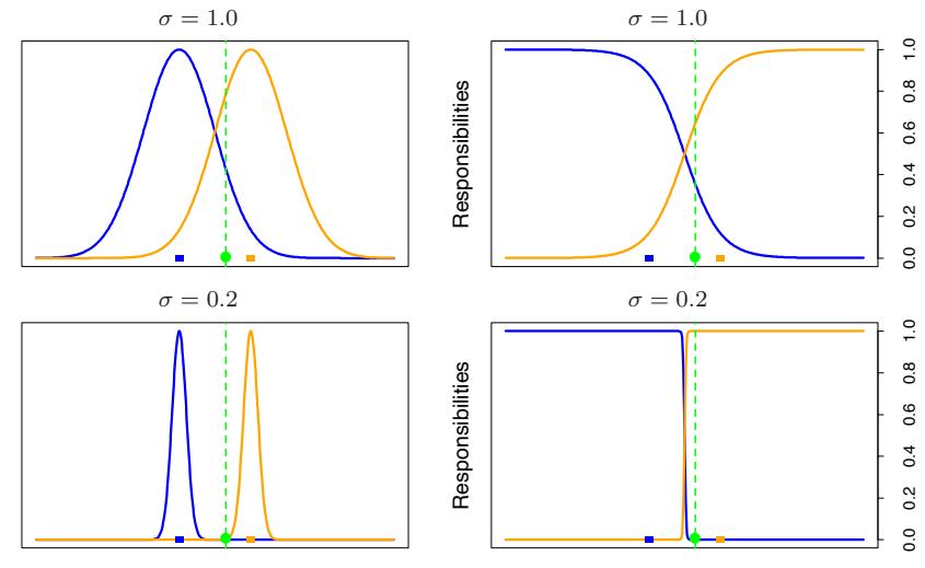
FIGURE 14.7. (Left panels:) two Gaussian densities g0(x) and g1(x) (blue and orange) on the real line, and a single data point (green dot) at x = 0.5. The colored squares are plotted at x = −1.0 and x = 1.0, the means of each density. (Right panels:) the relative densities g0(x)/(g0(x) + g1(x)) and g1(x)/(g0(x) + g1(x)), called the “responsibilities” of each cluster, for this data point. In the top panels, the Gaussian standard deviation σ = 1.0; in the bottom panels σ = 0.2. The EM algorithm uses these responsibilities to make a “soft” assignment of each data point to each of the two clusters. When σ is fairly large, the responsibilities can be near 0.5 (they are 0.36 and 0.64 in the top right panel). As σ → 0, the responsibilities → 1, for the cluster center closest to the target point, and 0 for all other clusters. This “hard” assignment is seen in the bottom right panel.

The E-step of the EM algorithm assigns “responsibilities” for each data point based in its relative density under each mixture component, while the M-step recomputes the component density parameters based on the current responsibilities. Suppose we specify K mixture components, each with a Gaussian density having scalar covariance matrix σ²I. Then the relative density under each mixture component is a monotone function of the Euclidean distance between the data point and the mixture center. Hence in this setup EM is a “soft” version of K-means clustering, making probabilistic (rather than deterministic) assignments of points to cluster centers. As the variance ^{σ2 →} 0, these probabilities become 0 and 1, and the two methods coincide. Details are given in Exercise 14.2. Figure 14.7 illustrates this result for two clusters on the real line.

14.3.8 Example: Human Tumor Microarray Data

We apply K-means clustering to the human tumor microarray data described in Chapter 1. This is an example of high-dimensional clustering.

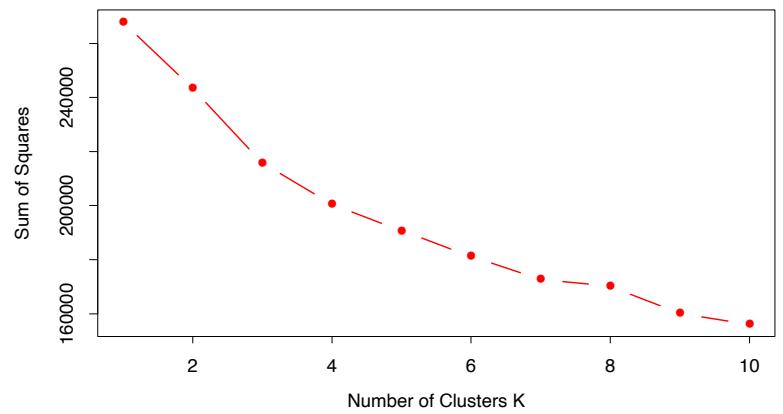
FIGURE 14.8. Total within-cluster sum of squares for K-means clustering applied to the human tumor microarray data.

TABLE 14.2. Human tumor data: number of cancer cases of each type, in each of the three clusters from K-means clustering.

Cluster	Breast	CNS	Colon	K562	Leukemia	MCF7
1	3	5	0	0	0	0
2	2	0	0	2	6	2
3	2	0	7	0	0	0
Cluster	Melanoma	NSCLC	Ovarian	Prostate	Renal	Unknown
1	1	7	6	2	9	1
2	7	2	0	0	0	0
3	0	0	0	0	0	0

The data are a 6830 × 64 matrix of real numbers, each representing an expression measurement for a gene (row) and sample (column). Here we cluster the samples, each of which is a vector of length 6830, corresponding to expression values for the 6830 genes. Each sample has a label such as breast (for breast cancer), melanoma, and so on; we don’t use these labels in the clustering, but will examine posthoc which labels fall into which clusters.

We applied K-means clustering with K running from 1 to 10, and computed the total within-sum of squares for each clustering, shown in Figure 14.8. Typically one looks for a kink in the sum of squares curve (or its logarithm) to locate the optimal number of clusters (see Section 14.3.11). Here there is no clear indication: for illustration we chose K = 3 giving the three clusters shown in Table 14.2.

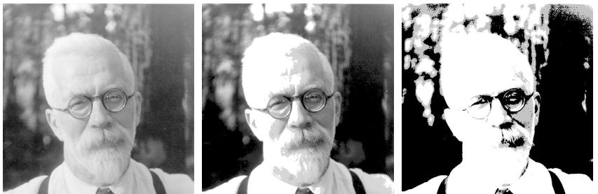
FIGURE 14.9. Sir Ronald A. Fisher (1890 − 1962) was one of the founders of modern day statistics, to whom we owe maximum-likelihood, sufficiency, and many other fundamental concepts. The image on the left is a 1024×1024 grayscale image at 8 bits per pixel. The center image is the result of 2 × 2 block VQ, using 200 code vectors, with a compression rate of 1.9 bits/pixel. The right image uses only four code vectors, with a compression rate of 0.50 bits/pixel

We see that the procedure is successful at grouping together samples of the same cancer. In fact, the two breast cancers in the second cluster were later found to be misdiagnosed and were melanomas that had metastasized. However, K-means clustering has shortcomings in this application. For one, it does not give a linear ordering of objects within a cluster: we have simply listed them in alphabetic order above. Secondly, as the number of clusters K is changed, the cluster memberships can change in arbitrary ways. That is, with say four clusters, the clusters need not be nested within the three clusters above. For these reasons, hierarchical clustering (described later), is probably preferable for this application.

14.3.9 Vector Quantization

The K-means clustering algorithm represents a key tool in the apparently unrelated area of image and signal compression, particularly in vector quantization or VQ (Gersho and Gray, 1992). The left image in Figure 14.9² is a digitized photograph of a famous statistician, Sir Ronald Fisher. It consists of 1024 × 1024 pixels, where each pixel is a grayscale value ranging from 0 to 255, and hence requires 8 bits of storage per pixel. The entire image occupies 1 megabyte of storage. The center image is a VQ-compressed version of the left panel, and requires 0.239 of the storage (at some loss in quality). The right image is compressed even more, and requires only 0.0625 of the storage (at a considerable loss in quality).

The version of VQ implemented here first breaks the image into small blocks, in this case 2×2 blocks of pixels. Each of the 512×512 blocks of four

²This example was prepared by Maya Gupta.

numbers is regarded as a vector in IR4. A K-means clustering algorithm (also known as Lloyd’s algorithm in this context) is run in this space. The center image uses K = 200, while the right image K = 4. Each of the 512×512 pixel blocks (or points) is approximated by its closest cluster centroid, known as a codeword. The clustering process is called the encoding step, and the collection of centroids is called the codebook.

To represent the approximated image, we need to supply for each block the identity of the codebook entry that approximates it. This will require log2(K) bits per block. We also need to supply the codebook itself, which is K × 4 real numbers (typically negligible). Overall, the storage for the compressed image amounts to log2(K)/(4 · 8) of the original (0.239 for K = 200, 0.063 for K = 4). This is typically expressed as a rate in bits per pixel: log2(K)/4, which are 1.91 and 0.50, respectively. The process of constructing the approximate image from the centroids is called the decoding step.

Why do we expect VQ to work at all? The reason is that for typical everyday images like photographs, many of the blocks look the same. In this case there are many almost pure white blocks, and similarly pure gray blocks of various shades. These require only one block each to represent them, and then multiple pointers to that block.

What we have described is known as lossy compression, since our images are degraded versions of the original. The degradation or distortion is usually measured in terms of mean squared error. In this case D = 0.89 for K = 200 and D = 16.95 for K = 4. More generally a rate/distortion curve would be used to assess the tradeoff. One can also perform lossless compression using block clustering, and still capitalize on the repeated patterns. If you took the original image and losslessly compressed it, the best you would do is 4.48 bits per pixel.

We claimed above that log2(K) bits were needed to identify each of the K codewords in the codebook. This uses a fixed-length code, and is inefficient if some codewords occur many more times than others in the image. Using Shannon coding theory, we know that in general a variable length code will do better, and the rate then becomes ⁻#^{K ℓ}=1 p^ℓ log2(pℓ)/4. The term in the numerator is the entropy of the distribution p^ℓ of the codewords in the image. Using variable length coding our rates come down to 1.42 and 0.39, respectively. Finally, there are many generalizations of VQ that have been developed: for example, tree-structured VQ finds the centroids with a top-down, 2-means style algorithm, as alluded to in Section 14.3.12. This allows successive refinement of the compression. Further details may be found in Gersho and Gray (1992).

14.3.10 K-medoids

As discussed above, the K-means algorithm is appropriate when the dissimilarity measure is taken to be squared Euclidean distance D(xi, xi′ )

516 14. Unsupervised Learning

Algorithm 14.2 K-medoids Clustering.

1. For a given cluster assignment C find the observation in the cluster minimizing total distance to other points in that cluster:

\[i\_k^\* = \underset{\{i: C(i) = k\}}{\text{argmin}} \sum\_{C(i') = k} D(x\_i, x\_{i'}).\tag{14.35}\]

Then m^k = xi^{∗ k} , k = 1, 2,…,K are the current estimates of the cluster centers.

2. Given a current set of cluster centers {m1,…,mK}, minimize the total error by assigning each observation to the closest (current) cluster center:

\[C(i) = \underset{1 \le k \le K}{\text{argmin}} \, D(x\_i, m\_k). \tag{14.36}\]

3. Iterate steps 1 and 2 until the assignments do not change.

(14.112). This requires all of the variables to be of the quantitative type. In addition, using squared Euclidean distance places the highest influence on the largest distances. This causes the procedure to lack robustness against outliers that produce very large distances. These restrictions can be removed at the expense of computation.

The only part of the K-means algorithm that assumes squared Euclidean distance is the minimization step (14.32); the cluster representatives {m1,…,mK} in (14.33) are taken to be the means of the currently assigned clusters. The algorithm can be generalized for use with arbitrarily defined dissimilarities D(xi, xi′ ) by replacing this step by an explicit optimization with respect to {m1,…,mK} in (14.33). In the most common form, centers for each cluster are restricted to be one of the observations assigned to the cluster, as summarized in Algorithm 14.2. This algorithm assumes attribute data, but the approach can also be applied to data described only by proximity matrices (Section 14.3.1). There is no need to explicitly compute cluster centers; rather we just keep track of the indices i ∗ k.

Solving (14.32) for each provisional cluster k requires an amount of computation proportional to the number of observations assigned to it, whereas for solving (14.35) the computation increases to O(N^{2 k} ). Given a set of cluster “centers,” {i1,…,iK}, obtaining the new assignments

\[C(i) = \operatorname\*{argmin}\_{1 \le k \le K} d\_{ii\_k^\*} \tag{14.37}\]

requires computation proportional to K · N as before. Thus, K-medoids is far more computationally intensive than K-means.

Alternating between (14.35) and (14.37) represents a particular heuristic search strategy for trying to solve

		BEL BRA CHI CUB EGY FRA IND						ISR			USA USS YUG
BRA	5.58
CHI	7.00	6.50
CUB	7.08	7.00	3.83
EGY	4.83	5.08	8.17	5.83
FRA	2.17	5.75	6.67	6.92	4.92
IND	6.42	5.00	5.58	6.00	4.67	6.42
ISR	3.42	5.50	6.42	6.42	5.00	3.92	6.17
USA	2.50	4.92	6.25	7.33	4.50	2.25	6.33	2.75
USS	6.08	6.67	4.25	2.67	6.00	6.17	6.17	6.92	6.17
YUG	5.25	6.83	4.50	3.75	5.75	5.42	6.08	5.83	6.67	3.67
ZAI	4.75	3.00	6.08	6.67	5.00	5.58	4.83	6.17	5.67	6.50	6.92

TABLE 14.3. Data from a political science survey: values are average pairwise dissimilarities of countries from a questionnaire given to political science students.

\[\min\_{C, \{i\_k\}\_1^K} \sum\_{k=1}^K \sum\_{C(i)=k} d\_{ii\_k}. \tag{14.38}\]

Kaufman and Rousseeuw (1990) propose an alternative strategy for directly solving (14.38) that provisionally exchanges each center i^k with an observation that is not currently a center, selecting the exchange that produces the greatest reduction in the value of the criterion (14.38). This is repeated until no advantageous exchanges can be found. Massart et al. (1983) derive a branch-and-bound combinatorial method that finds the global minimum of (14.38) that is practical only for very small data sets.

Example: Country Dissimilarities

This example, taken from Kaufman and Rousseeuw (1990), comes from a study in which political science students were asked to provide pairwise dissimilarity measures for 12 countries: Belgium, Brazil, Chile, Cuba, Egypt, France, India, Israel, United States, Union of Soviet Socialist Republics, Yugoslavia and Zaire. The average dissimilarity scores are given in Table 14.3. We applied 3-medoid clustering to these dissimilarities. Note that K-means clustering could not be applied because we have only distances rather than raw observations. The left panel of Figure 14.10 shows the dissimilarities reordered and blocked according to the 3-medoid clustering. The right panel is a two-dimensional multidimensional scaling plot, with the 3-medoid clusters assignments indicated by colors (multidimensional scaling is discussed in Section 14.8.) Both plots show three well-separated clusters, but the MDS display indicates that “Egypt” falls about halfway between two clusters.

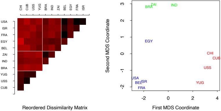
FIGURE 14.10. Survey of country dissimilarities. (Left panel:) dissimilarities reordered and blocked according to 3-medoid clustering. Heat map is coded from most similar (dark red) to least similar (bright red). (Right panel:) two-dimensional multidimensional scaling plot, with 3-medoid clusters indicated by different colors.

14.3.11 Practical Issues

In order to apply K-means or K-medoids one must select the number of clusters K^∗ and an initialization. The latter can be defined by specifying an initial set of centers {m1,…,mK} or {i1,…,iK} or an initial encoder C(i). Usually specifying the centers is more convenient. Suggestions range from simple random selection to a deliberate strategy based on forward stepwise assignment. At each step a new center i^k is chosen to minimize the criterion (14.33) or (14.38), given the centers i1,…,ik−¹ chosen at the previous steps. This continues for K steps, thereby producing K initial centers with which to begin the optimization algorithm.

A choice for the number of clusters K depends on the goal. For data segmentation K is usually defined as part of the problem. For example, a company may employ K sales people, and the goal is to partition a customer database into K segments, one for each sales person, such that the customers assigned to each one are as similar as possible. Often, however, cluster analysis is used to provide a descriptive statistic for ascertaining the extent to which the observations comprising the data base fall into natural distinct groupings. Here the number of such groups K^∗ is unknown and one requires that it, as well as the groupings themselves, be estimated from the data.

Data-based methods for estimating K^∗ typically examine the withincluster dissimilarity W^K as a function of the number of clusters K. Separate solutions are obtained for K ∈ {1, 2,…,Kmax}. The corresponding values {W1, W2,…,WKmax } generally decrease with increasing K. This will be the case even when the criterion is evaluated on an independent test set, since a large number of cluster centers will tend to fill the feature space densely and thus will be close to all data points. Thus cross-validation techniques, so useful for model selection in supervised learning, cannot be utilized in this context.

The intuition underlying the approach is that if there are actually K^∗ distinct groupings of the observations (as defined by the dissimilarity measure), then for K<K^∗ the clusters returned by the algorithm will each contain a subset of the true underlying groups. That is, the solution will not assign observations in the same naturally occurring group to different estimated clusters. To the extent that this is the case, the solution criterion value will tend to decrease substantially with each successive increase in the number of specified clusters, WK+1 ≪ WK, as the natural groups are successively assigned to separate clusters. For K>K^∗, one of the estimated clusters must partition at least one of the natural groups into two subgroups. This will tend to provide a smaller decrease in the criterion as K is further increased. Splitting a natural group, within which the observations are all quite close to each other, reduces the criterion less than partitioning the union of two well-separated groups into their proper constituents.

To the extent this scenario is realized, there will be a sharp decrease in successive differences in criterion value, ^{WK − W}K+1, at ^{K = K∗}. That is, {W^{K − W}K+1 ^| K<K^∗} ^≫ {W^{K − W}K+1 ^{| K ≥ K∗}}. An estimate Kˆ ^∗ for K^∗ is then obtained by identifying a “kink” in the plot of W^K as a function of K. As with other aspects of clustering procedures, this approach is somewhat heuristic.

The recently proposed Gap statistic (Tibshirani et al., 2001b) compares the curve log W^K to the curve obtained from data uniformly distributed over a rectangle containing the data. It estimates the optimal number of clusters to be the place where the gap between the two curves is largest. Essentially this is an automatic way of locating the aforementioned “kink.” It also works reasonably well when the data fall into a single cluster, and in that case will tend to estimate the optimal number of clusters to be one. This is the scenario where most other competing methods fail.

Figure 14.11 shows the result of the Gap statistic applied to simulated data of Figure 14.4. The left panel shows log W^K for k = 1, 2,…, 8 clusters (green curve) and the expected value of log W^K over 20 simulations from uniform data (blue curve). The right panel shows the gap curve, which is the expected curve minus the observed curve. Shown also are error bars of halfwidth s′ ^K = s^K O1+1/20, where s^K is the standard deviation of log W^K over the 20 simulations. The Gap curve is maximized at K = 2 clusters. If G(K) is the Gap curve at K clusters, the formal rule for estimating K^∗ is

\[K^\* = \underset{K}{\text{argmin}} \{ K | G(K) \ge G(K+1) - s\_{K+1}' \}. \tag{14.39}\]

FIGURE 14.11. (Left panel): observed (green) and expected (blue) values of log W^K for the simulated data of Figure 14.4. Both curves have been translated to equal zero at one cluster. (Right panel): Gap curve, equal to the difference between the observed and expected values of log WK. The Gap estimate K^∗ is the smallest K producing a gap within one standard deviation of the gap at K + 1; here K^∗ = 2.

This gives K^∗ = 2, which looks reasonable from Figure 14.4.

14.3.12 Hierarchical Clustering

The results of applying K-means or K-medoids clustering algorithms depend on the choice for the number of clusters to be searched and a starting configuration assignment. In contrast, hierarchical clustering methods do not require such specifications. Instead, they require the user to specify a measure of dissimilarity between (disjoint) groups of observations, based on the pairwise dissimilarities among the observations in the two groups. As the name suggests, they produce hierarchical representations in which the clusters at each level of the hierarchy are created by merging clusters at the next lower level. At the lowest level, each cluster contains a single observation. At the highest level there is only one cluster containing all of the data.

Strategies for hierarchical clustering divide into two basic paradigms: agglomerative (bottom-up) and divisive (top-down). Agglomerative strategies start at the bottom and at each level recursively merge a selected pair of clusters into a single cluster. This produces a grouping at the next higher level with one less cluster. The pair chosen for merging consist of the two groups with the smallest intergroup dissimilarity. Divisive methods start at the top and at each level recursively split one of the existing clusters at that level into two new clusters. The split is chosen to produce two new groups with the largest between-group dissimilarity. With both paradigms there are N − 1 levels in the hierarchy.

Each level of the hierarchy represents a particular grouping of the data into disjoint clusters of observations. The entire hierarchy represents an ordered sequence of such groupings. It is up to the user to decide which level (if any) actually represents a “natural” clustering in the sense that observations within each of its groups are sufficiently more similar to each other than to observations assigned to different groups at that level. The Gap statistic described earlier can be used for this purpose.

Recursive binary splitting/agglomeration can be represented by a rooted binary tree. The nodes of the trees represent groups. The root node represents the entire data set. The N terminal nodes each represent one of the individual observations (singleton clusters). Each nonterminal node (“parent”) has two daughter nodes. For divisive clustering the two daughters represent the two groups resulting from the split of the parent; for agglomerative clustering the daughters represent the two groups that were merged to form the parent.

All agglomerative and some divisive methods (when viewed bottom-up) possess a monotonicity property. That is, the dissimilarity between merged clusters is monotone increasing with the level of the merger. Thus the binary tree can be plotted so that the height of each node is proportional to the value of the intergroup dissimilarity between its two daughters. The terminal nodes representing individual observations are all plotted at zero height. This type of graphical display is called a dendrogram.

A dendrogram provides a highly interpretable complete description of the hierarchical clustering in a graphical format. This is one of the main reasons for the popularity of hierarchical clustering methods.

For the microarray data, Figure 14.12 shows the dendrogram resulting from agglomerative clustering with average linkage; agglomerative clustering and this example are discussed in more detail later in this chapter. Cutting the dendrogram horizontally at a particular height partitions the data into disjoint clusters represented by the vertical lines that intersect it. These are the clusters that would be produced by terminating the procedure when the optimal intergroup dissimilarity exceeds that threshold cut value. Groups that merge at high values, relative to the merger values of the subgroups contained within them lower in the tree, are candidates for natural clusters. Note that this may occur at several different levels, indicating a clustering hierarchy: that is, clusters nested within clusters.

Such a dendrogram is often viewed as a graphical summary of the data itself, rather than a description of the results of the algorithm. However, such interpretations should be treated with caution. First, different hierarchical methods (see below), as well as small changes in the data, can lead to quite different dendrograms. Also, such a summary will be valid only to the extent that the pairwise observation dissimilarities possess the hierar-

FIGURE 14.12. Dendrogram from agglomerative hierarchical clustering with average linkage to the human tumor microarray data.

chical structure produced by the algorithm. Hierarchical methods impose hierarchical structure whether or not such structure actually exists in the data.

The extent to which the hierarchical structure produced by a dendrogram actually represents the data itself can be judged by the cophenetic correlation coefficient. This is the correlation between the N(N −1)/2 pairwise observation dissimilarities dii′ input to the algorithm and their corresponding cophenetic dissimilarities Cii′ derived from the dendrogram. The cophenetic dissimilarity Cii′ between two observations (i, i′ ) is the intergroup dissimilarity at which observations i and i ′ are first joined together in the same cluster.

The cophenetic dissimilarity is a very restrictive dissimilarity measure. First, the Cii′ over the observations must contain many ties, since only N−1 of the total N(N − 1)/2 values can be distinct. Also these dissimilarities obey the ultrametric inequality

\[C\_{ii'} \le \max\{C\_{ik}, C\_{i'k}\} \tag{14.40}\]

for any three observations (i, i′ , k). As a geometric example, suppose the data were represented as points in a Euclidean coordinate system. In order for the set of interpoint distances over the data to conform to (14.40), the triangles formed by all triples of points must be isosceles triangles with the unequal length no longer than the length of the two equal sides (Jain and Dubes, 1988). Therefore it is unrealistic to expect general dissimilarities over arbitrary data sets to closely resemble their corresponding cophenetic dissimilarities as calculated from a dendrogram, especially if there are not many tied values. Thus the dendrogram should be viewed mainly as a description of the clustering structure of the data as imposed by the particular algorithm employed.

Agglomerative Clustering

Agglomerative clustering algorithms begin with every observation representing a singleton cluster. At each of the N −1 steps the closest two (least dissimilar) clusters are merged into a single cluster, producing one less cluster at the next higher level. Therefore, a measure of dissimilarity between two clusters (groups of observations) must be defined.

Let G and H represent two such groups. The dissimilarity d(G, H) between G and H is computed from the set of pairwise observation dissimilarities dii′ where one member of the pair i is in G and the other i ′ is in H. Single linkage (SL) agglomerative clustering takes the intergroup dissimilarity to be that of the closest (least dissimilar) pair

\[d\_{SL}(G,H) = \min\_{\substack{i \in G \\ i' \in H}} d\_{ii'}.\tag{14.41}\]

This is also often called the nearest-neighbor technique. Complete linkage (CL) agglomerative clustering (furthest-neighbor technique) takes the intergroup dissimilarity to be that of the furthest (most dissimilar) pair

\[d\_{CL}(G, H) = \max\_{\substack{i \in G \\ i' \in H}} d\_{ii'}.\tag{14.42}\]

Group average (GA) clustering uses the average dissimilarity between the groups

\[d\_{GA}(G,H) = \frac{1}{N\_G N\_H} \sum\_{i \in G} \sum\_{i' \in H} d\_{ii'} \tag{14.43}\]

where N^G and N^H are the respective number of observations in each group. Although there have been many other proposals for defining intergroup dissimilarity in the context of agglomerative clustering, the above three are the ones most commonly used. Figure 14.13 shows examples of all three.

If the data dissimilarities {dii′} exhibit a strong clustering tendency, with each of the clusters being compact and well separated from others, then all three methods produce similar results. Clusters are compact if all of the

FIGURE 14.13. Dendrograms from agglomerative hierarchical clustering of human tumor microarray data.

observations within them are relatively close together (small dissimilarities) as compared with observations in different clusters. To the extent this is not the case, results will differ.

Single linkage (14.41) only requires that a single dissimilarity dii′ , i ∈ G and i ′ ^{∈ H}, be small for two groups ^G and ^H to be considered close together, irrespective of the other observation dissimilarities between the groups. It will therefore have a tendency to combine, at relatively low thresholds, observations linked by a series of close intermediate observations. This phenomenon, referred to as chaining, is often considered a defect of the method. The clusters produced by single linkage can violate the “compactness” property that all observations within each cluster tend to be similar to one another, based on the supplied observation dissimilarities {dii′}. If we define the diameter D^G of a group of observations as the largest dissimilarity among its members

\[D\_G = \max\_{\substack{i \in G \\ i' \in G}} d\_{ii'}, \tag{14.44}\]

then single linkage can produce clusters with very large diameters.

Complete linkage (14.42) represents the opposite extreme. Two groups G and H are considered close only if all of the observations in their union are relatively similar. It will tend to produce compact clusters with small diameters (14.44). However, it can produce clusters that violate the “closeness” property. That is, observations assigned to a cluster can be much closer to members of other clusters than they are to some members of their own cluster.

Group average clustering (14.43) represents a compromise between the two extremes of single and complete linkage. It attempts to produce relatively compact clusters that are relatively far apart. However, its results depend on the numerical scale on which the observation dissimilarities dii′ are measured. Applying a monotone strictly increasing transformation h(·) to the dii′ , hii′ = h(dii′ ), can change the result produced by (14.43). In contrast, (14.41) and (14.42) depend only on the ordering of the dii′ and are thus invariant to such monotone transformations. This invariance is often used as an argument in favor of single or complete linkage over group average methods.

One can argue that group average clustering has a statistical consistency property violated by single and complete linkage. Assume we have attribute-value data X^T = (X1,…,Xp) and that each cluster k is a random sample from some population joint density pk(x). The complete data set is a random sample from a mixture of K such densities. The group average dissimilarity dGA(G, H) (14.43) is an estimate of

\[ \int \int d(x, x') \, p\_G(x) \, p\_H(x') \, dx \, dx',\tag{14.45} \]

where d(x, x′ ) is the dissimilarity between points x and x′ in the space of attribute values. As the sample size N approaches infinity dGA(G, H) (14.43) approaches (14.45), which is a characteristic of the relationship between the two densities pG(x) and pH(x) . For single linkage, dSL(G, H) (14.41) approaches zero as N → ∞ independent of pG(x) and pH(x) . For complete linkage, dCL(G, H) (14.42) becomes infinite as N → ∞, again independent of the two densities. Thus, it is not clear what aspects of the population distribution are being estimated by dSL(G, H) and dCL(G, H).

Example: Human Cancer Microarray Data (Continued)

The left panel of Figure 14.13 shows the dendrogram resulting from average linkage agglomerative clustering of the samples (columns) of the microarray data. The middle and right panels show the result using complete and single linkage. Average and complete linkage gave similar results, while single linkage produced unbalanced groups with long thin clusters. We focus on the average linkage clustering.

Like K-means clustering, hierarchical clustering is successful at clustering simple cancers together. However it has other nice features. By cutting off the dendrogram at various heights, different numbers of clusters emerge, and the sets of clusters are nested within one another. Secondly, it gives some partial ordering information about the samples. In Figure 14.14, we have arranged the genes (rows) and samples (columns) of the expression matrix in orderings derived from hierarchical clustering.

526 14. Unsupervised Learning

Note that if we flip the orientation of the branches of a dendrogram at any merge, the resulting dendrogram is still consistent with the series of hierarchical clustering operations. Hence to determine an ordering of the leaves, we must add a constraint. To produce the row ordering of Figure 14.14, we have used the default rule in S-PLUS: at each merge, the subtree with the tighter cluster is placed to the left (toward the bottom in the rotated dendrogram in the figure.) Individual genes are the tightest clusters possible, and merges involving two individual genes place them in order by their observation number. The same rule was used for the columns. Many other rules are possible—for example, ordering by a multidimensional scaling of the genes; see Section 14.8.

The two-way rearrangement of Figure14.14 produces an informative picture of the genes and samples. This picture is more informative than the randomly ordered rows and columns of Figure 1.3 of Chapter 1. Furthermore, the dendrograms themselves are useful, as biologists can, for example, interpret the gene clusters in terms of biological processes.

Divisive Clustering

Divisive clustering algorithms begin with the entire data set as a single cluster, and recursively divide one of the existing clusters into two daughter clusters at each iteration in a top-down fashion. This approach has not been studied nearly as extensively as agglomerative methods in the clustering literature. It has been explored somewhat in the engineering literature (Gersho and Gray, 1992) in the context of compression. In the clustering setting, a potential advantage of divisive over agglomerative methods can occur when interest is focused on partitioning the data into a relatively small number of clusters.

The divisive paradigm can be employed by recursively applying any of the combinatorial methods such as K-means (Section 14.3.6) or K-medoids (Section 14.3.10), with K = 2, to perform the splits at each iteration. However, such an approach would depend on the starting configuration specified at each step. In addition, it would not necessarily produce a splitting sequence that possesses the monotonicity property required for dendrogram representation.

A divisive algorithm that avoids these problems was proposed by Macnaughton Smith et al. (1965). It begins by placing all observations in a single cluster G. It then chooses that observation whose average dissimilarity from all the other observations is largest. This observation forms the first member of a second cluster H. At each successive step that observation in G whose average distance from those in H, minus that for the remaining observations in G is largest, is transferred to H. This continues until the corresponding difference in averages becomes negative. That is, there are no longer any observations in G that are, on average, closer to those in H. The result is a split of the original cluster into two daughter clusters,

FIGURE 14.14. DNA microarray data: average linkage hierarchical clustering has been applied independently to the rows (genes) and columns (samples), determining the ordering of the rows and columns (see text). The colors range from bright green (negative, under-expressed) to bright red (positive, over-expressed).

528 14. Unsupervised Learning

the observations transferred to H, and those remaining in G. These two clusters represent the second level of the hierarchy. Each successive level is produced by applying this splitting procedure to one of the clusters at the previous level. Kaufman and Rousseeuw (1990) suggest choosing the cluster at each level with the largest diameter (14.44) for splitting. An alternative would be to choose the one with the largest average dissimilarity among its members

\[\bar{d}\_G = \frac{1}{N\_G} \sum\_{i \in G} \sum\_{i' \in G} d\_{ii'} \dots\]

The recursive splitting continues until all clusters either become singletons or all members of each one have zero dissimilarity from one another.

14.4 Self-Organizing Maps

This method can be viewed as a constrained version of K-means clustering, in which the prototypes are encouraged to lie in a one- or two-dimensional manifold in the feature space. The resulting manifold is also referred to as a constrained topological map, since the original high-dimensional observations can be mapped down onto the two-dimensional coordinate system. The original SOM algorithm was online—observations are processed one at a time—and later a batch version was proposed. The technique also bears a close relationship to principal curves and surfaces, which are discussed in the next section.

We consider a SOM with a two-dimensional rectangular grid of K prototypes ^{mj ∈} IR^p (other choices, such as hexagonal grids, can also be used). Each of the K prototypes are parametrized with respect to an integer coordinate pair ℓ^j ∈ Q¹ × Q2. Here Q¹ = {1, 2,…,q1}, similarly Q2, and K = q1·q2. The m^j are initialized, for example, to lie in the two-dimensional principal component plane of the data (next section). We can think of the prototypes as “buttons,” “sewn” on the principal component plane in a regular pattern. The SOM procedure tries to bend the plane so that the buttons approximate the data points as well as possible. Once the model is fit, the observations can be mapped down onto the two-dimensional grid.

The observations xⁱ are processed one at a time. We find the closest prototype m^j to xⁱ in Euclidean distance in IRp, and then for all neighbors m^k of m^j , move m^k toward xⁱ via the update

\[m\_k \gets m\_k + \alpha (x\_i - m\_k). \tag{14.46}\]

The “neighbors” of m^j are defined to be all m^k such that the distance between ℓ^j and ℓ^k is small. The simplest approach uses Euclidean distance, and “small” is determined by a threshold r. This neighborhood always includes the closest prototype m^j itself.

Notice that distance is defined in the space Q1×Q² of integer topological coordinates of the prototypes, rather than in the feature space IRp. The effect of the update (14.46) is to move the prototypes closer to the data, but also to maintain a smooth two-dimensional spatial relationship between the prototypes.

The performance of the SOM algorithm depends on the learning rate α and the distance threshold r. Typically α is decreased from say 1.0 to 0.0 over a few thousand iterations (one per observation). Similarly r is decreased linearly from starting value R to 1 over a few thousand iterations. We illustrate a method for choosing R in the example below.

We have described the simplest version of the SOM. More sophisticated versions modify the update step according to distance:

\[m\_k \gets m\_k + \alpha h (||\ell\_j - \ell\_k||) (x\_i - m\_k),\tag{14.47}\]

where the neighborhood function h gives more weight to prototypes m^k with indices ℓ^k closer to ℓ^j than to those further away.

If we take the distance r small enough so that each neighborhood contains only one point, then the spatial connection between prototypes is lost. In that case one can show that the SOM algorithm is an online version of K-means clustering, and eventually stabilizes at one of the local minima found by K-means. Since the SOM is a constrained version of K-means clustering, it is important to check whether the constraint is reasonable in any given problem. One can do this by computing the reconstruction error ^{∥x − m}j∥², summed over observations, for both methods. This will necessarily be smaller for K-means, but should not be much smaller if the SOM is a reasonable approximation.

As an illustrative example, we generated 90 data points in three dimensions, near the surface of a half sphere of radius 1. The points were in each of three clusters—red, green, and blue—located near (0, 1, 0), (0, 0, 1) and (1, 0, 0). The data are shown in Figure 14.15

By design, the red cluster was much tighter than the green or blue ones. (Full details of the data generation are given in Exercise 14.5.) A 5×5 grid of prototypes was used, with initial grid size R = 2; this meant that about a third of the prototypes were initially in each neighborhood. We did a total of 40 passes through the dataset of 90 observations, and let r and α decrease linearly over the 3600 iterations.

In Figure 14.16 the prototypes are indicated by circles, and the points that project to each prototype are plotted randomly within the corresponding circle. The left panel shows the initial configuration, while the right panel shows the final one. The algorithm has succeeded in separating the clusters; however, the separation of the red cluster indicates that the manifold has folded back on itself (see Figure 14.17). Since the distances in the two-dimensional display are not used, there is little indication in the SOM projection that the red cluster is tighter than the others.

FIGURE 14.15. Simulated data in three classes, near the surface of a half– sphere.

FIGURE 14.16. Self-organizing map applied to half-sphere data example. Left panel is the initial configuration, right panel the final one. The 5 × 5 grid of prototypes are indicated by circles, and the points that project to each prototype are plotted randomly within the corresponding circle.

FIGURE 14.17. Wiremesh representation of the fitted SOM model in IR³. The lines represent the horizontal and vertical edges of the topological lattice. The double lines indicate that the surface was folded diagonally back on itself in order to model the red points. The cluster members have been jittered to indicate their color, and the purple points are the node centers.

Figure 14.18 shows the reconstruction error, equal to the total sum of squares of each data point around its prototype. For comparison we carried out a K-means clustering with 25 centroids, and indicate its reconstruction error by the horizontal line on the graph. We see that the SOM significantly decreases the error, nearly to the level of the K-means solution. This provides evidence that the two-dimensional constraint used by the SOM is reasonable for this particular dataset.

In the batch version of the SOM, we update each m^j via

\[m\_j = \frac{\sum w\_k x\_k}{\sum w\_k}.\tag{14.48}\]

The sum is over points x^k that mapped (i.e., were closest to) neighbors m^k of m^j . The weight function may be rectangular, that is, equal to 1 for the neighbors of mk, or may decrease smoothly with distance ∥ℓk−ℓj∥ as before. If the neighborhood size is chosen small enough so that it consists only of mk, with rectangular weights, this reduces to the K-means clustering procedure described earlier. It can also be thought of as a discrete version of principal curves and surfaces, described in Section 14.5.

FIGURE 14.18. Half-sphere data: reconstruction error for the SOM as a function of iteration. Error for k-means clustering is indicated by the horizontal line.

Example: Document Organization and Retrieval

Document retrieval has gained importance with the rapid development of the Internet and the Web, and SOMs have proved to be useful for organizing and indexing large corpora. This example is taken from the WEBSOM homepage http://websom.hut.fi/ (Kohonen et al., 2000). Figure 14.19 represents a SOM fit to 12,088 newsgroup comp.ai.neural-nets articles. The labels are generated automatically by the WEBSOM software and provide a guide as to the typical content of a node.

In applications such as this, the documents have to be reprocessed in order to create a feature vector. A term-document matrix is created, where each row represents a single document. The entries in each row are the relative frequency of each of a predefined set of terms. These terms could be a large set of dictionary entries (50,000 words), or an even larger set of bigrams (word pairs), or subsets of these. These matrices are typically very sparse, and so often some preprocessing is done to reduce the number of features (columns). Sometimes the SVD (next section) is used to reduce the matrix; Kohonen et al. (2000) use a randomized variant thereof. These reduced vectors are then the input to the SOM.

FIGURE 14.19. Heatmap representation of the SOM model fit to a corpus of 12,088 newsgroup comp.ai.neural-nets contributions (courtesy WEBSOM homepage). The lighter areas indicate higher-density areas. Populated nodes are automatically labeled according to typical content.

FIGURE 14.20. The first linear principal component of a set of data. The line minimizes the total squared distance from each point to its orthogonal projection onto the line.

In this application the authors have developed a “zoom” feature, which allows one to interact with the map in order to get more detail. The final level of zooming retrieves the actual news articles, which can then be read.

14.5 Principal Components, Curves and Surfaces

Principal components are discussed in Sections 3.4.1, where they shed light on the shrinkage mechanism of ridge regression. Principal components are a sequence of projections of the data, mutually uncorrelated and ordered in variance. In the next section we present principal components as linear manifolds approximating a set of ^N points ^{xi ∈} IR^p. We then present some nonlinear generalizations in Section 14.5.2. Other recent proposals for nonlinear approximating manifolds are discussed in Section 14.9.

14.5.1 Principal Components

The principal components of a set of data in IR^p provide a sequence of best linear approximations to that data, of all ranks q ≤ p.

Denote the observations by x1, x2,…,x^N , and consider the rank-q linear model for representing them

14.5 Principal Components, Curves and Surfaces 535

\[f(\lambda) = \mu + \mathbf{V}\_q \lambda,\tag{14.49}\]

where ^µ is a location vector in IRp, ^Vq is a ^{p × q} matrix with ^q orthogonal unit vectors as columns, and λ is a q vector of parameters. This is the parametric representation of an affine hyperplane of rank q. Figures 14.20 and 14.21 illustrate for q = 1 and q = 2, respectively. Fitting such a model to the data by least squares amounts to minimizing the reconstruction error

\[\min\_{\mu, \{\lambda\_i\}, \mathbf{V}\_q} \sum\_{i=1}^N \left\| x\_i - \mu - \mathbf{V}\_q \lambda\_i \right\|^2. \tag{14.50}\]

We can partially optimize for µ and the λⁱ (Exercise 14.7) to obtain

\[ \hat{\mu}\_{-} = \quad \bar{x}, \tag{14.51} \]

\[ \hat{\lambda}\_i \quad = \quad \mathbf{V}\_q^T (x\_i - \bar{x}). \tag{14.52} \]

This leaves us to find the orthogonal matrix Vq:

\[\min\_{\mathbf{V}\_q} \sum\_{i=1}^N ||(x\_i - \bar{x}) - \mathbf{V}\_q \mathbf{V}\_q^T (x\_i - \bar{x})||^2. \tag{14.53}\]

For convenience we assume that ¯x = 0 (otherwise we simply replace the observations by their centered versions ˜xⁱ = xⁱ − x¯). The p × p matrix H^q = VqV^{T q} is a projection matrix, and maps each point xⁱ onto its rankq reconstruction Hqxi, the orthogonal projection of xⁱ onto the subspace spanned by the columns of Vq. The solution can be expressed as follows. Stack the (centered) observations into the rows of an N × p matrix X. We construct the singular value decomposition of X:

\[\mathbf{X} = \mathbf{U}\mathbf{D}\mathbf{V}^T.\tag{14.54}\]

This is a standard decomposition in numerical analysis, and many algorithms exist for its computation (Golub and Van Loan, 1983, for example). Here ^U is an ^{N × p} orthogonal matrix (U^{T U = I}p) whose columns ^uj are called the left singular vectors; ^V is a ^p×^p orthogonal matrix (V^{T V = I}p) with columns v^j called the right singular vectors, and D is a p×p diagonal matrix, with diagonal elements d¹ ≥ d² ≥ ··· ≥ d^p ≥ 0 known as the singular values. For each rank q, the solution V^q to (14.53) consists of the first q columns of V. The columns of UD are called the principal components of X (see Section 3.5.1). The N optimal λˆⁱ in (14.52) are given by the first q principal components (the N rows of the N × q matrix UqDq).

The one-dimensional principal component line in IR² is illustrated in Figure 14.20. For each data point xi, there is a closest point on the line, given by ui1d1v1. Here v¹ is the direction of the line and λˆⁱ = ui1d¹ measures distance along the line from the origin. Similarly Figure 14.21 shows the

FIGURE 14.21. The best rank-two linear approximation to the half-sphere data. The right panel shows the projected points with coordinates given by U2D2, the first two principal components of the data.

two-dimensional principal component surface fit to the half-sphere data (left panel). The right panel shows the projection of the data onto the first two principal components. This projection was the basis for the initial configuration for the SOM method shown earlier. The procedure is quite successful at separating the clusters. Since the half-sphere is nonlinear, a nonlinear projection will do a better job, and this is the topic of the next section.

Principal components have many other nice properties, for example, the linear combination Xv¹ has the highest variance among all linear combinations of the features; Xv² has the highest variance among all linear combinations satisfying v² orthogonal to v1, and so on.

Example: Handwritten Digits

Principal components are a useful tool for dimension reduction and compression. We illustrate this feature on the handwritten digits data described in Chapter 1. Figure 14.22 shows a sample of 130 handwritten 3’s, each a digitized 16 × 16 grayscale image, from a total of 658 such 3’s. We see considerable variation in writing styles, character thickness and orientation. We consider these images as points xⁱ in IR256, and compute their principal components via the SVD (14.54).

Figure 14.23 shows the first two principal components of these data. For each of these first two principal components ui¹ and ui2, we computed the 5%, 25%, 50%, 75% and 95% quantile points, and used them to define the rectangular grid superimposed on the plot. The circled points indicate

FIGURE 14.22. A sample of 130 handwritten 3’s shows a variety of writing styles.

those images close to the vertices of the grid, where the distance measure focuses mainly on these projected coordinates, but gives some weight to the components in the orthogonal subspace. The right plot shows the images corresponding to these circled points. This allows us to visualize the nature of the first two principal components. We see that the v¹ (horizontal movement) mainly accounts for the lengthening of the lower tail of the three, while v² (vertical movement) accounts for character thickness. In terms of the parametrized model (14.49), this two-component model has the form

\[\begin{array}{rcl}\hat{f}(\lambda) &=& \bar{x} + \lambda\_1 v\_1 + \lambda\_2 v\_2\\ &=& \left[\underbrace{\begin{array}{c} \text{??} \\ \text{iii} \end{array} \right] + \lambda\_1 \cdot \left[\begin{array}{c} \text{??} \\ \text{iii} \end{array} \right] + \lambda\_2 \cdot \left[\begin{array}{c} \text{iii} \\ \text{iv} \end{array} \right]. \end{array} \tag{14.55}\]

Here we have displayed the first two principal component directions, v¹ and v2, as images. Although there are a possible 256 principal components, approximately 50 account for 90% of the variation in the threes, 12 account for 63%. Figure 14.24 compares the singular values to those obtained for equivalent uncorrelated data, obtained by randomly scrambling each column of X. The pixels in a digitized image are inherently correlated, and since these are all the same digit the correlations are even stronger.

FIGURE 14.23. (Left panel:) the first two principal components of the handwritten threes. The circled points are the closest projected images to the vertices of a grid, defined by the marginal quantiles of the principal components. (Right panel:) The images corresponding to the circled points. These show the nature of the first two principal components.

FIGURE 14.24. The 256 singular values for the digitized threes, compared to those for a randomized version of the data (each column of X was scrambled).

A relatively small subset of the principal components serve as excellent lower-dimensional features for representing the high-dimensional data.

Example: Procrustes Transformations and Shape Averaging

FIGURE 14.25. (Left panel:) Two different digitized handwritten Ss, each represented by 96 corresponding points in IR². The green S has been deliberately rotated and translated for visual effect. (Right panel:) A Procrustes transformation applies a translation and rotation to best match up the two set of points.

Figure 14.25 represents two sets of points, the orange and green, in the same plot. In this instance these points represent two digitized versions of a handwritten S, extracted from the signature of a subject “Suresh.” Figure 14.26 shows the entire signatures from which these were extracted (third and fourth panels). The signatures are recorded dynamically using touch-screen devices, familiar sights in modern supermarkets. There are N = 96 points representing each S, which we denote by the N ×2 matrices X¹ and X2. There is a correspondence between the points—the ith rows of X¹ and X² are meant to represent the same positions along the two S’s. In the language of morphometrics, these points represent landmarks on the two objects. How one finds such corresponding landmarks is in general difficult and subject specific. In this particular case we used dynamic time warping of the speed signal along each signature (Hastie et al., 1992), but will not go into details here.

In the right panel we have applied a translation and rotation to the green points so as best to match the orange—a so-called Procrustes³ transformation (Mardia et al., 1979, for example).

Consider the problem

\[\min\_{\boldsymbol{\mu}, \mathbf{R}} ||\mathbf{X}\_2 - (\mathbf{X}\_1 \mathbf{R} + \mathbf{1} \boldsymbol{\mu}^T)||\_F,\tag{14.56}\]

³Procrustes was an African bandit in Greek mythology, who stretched or squashed his visitors to fit his iron bed (eventually killing them).

540 14. Unsupervised Learning

with X¹ and X² both N × p matrices of corresponding points, R an orthonormal ^{p × p} matrix4, and ^{µ a p}-vector of location coordinates. Here ||X||^{2 F} = trace(X^T X) is the squared Frobenius matrix norm.

Let ¯x¹ and ¯x² be the column mean vectors of the matrices, and X˜ ¹ and X˜ ² be the versions of these matrices with the means removed. Consider the SVD X˜ ^{T 1} X˜ ² = UDV^T . Then the solution to (14.56) is given by (Exercise 14.8)

\[\begin{array}{rcl} \hat{\mathbf{R}} & = & \mathbf{U} \mathbf{V}^{T} \\ \hat{\boldsymbol{\mu}} & = & \bar{\boldsymbol{x}}\_{2} - \hat{\mathbf{R}} \bar{\boldsymbol{x}}\_{1}, \end{array} \tag{14.57}\]

and the minimal distances is referred to as the Procrustes distance. From the form of the solution, we can center each matrix at its column centroid, and then ignore location completely. Hereafter we assume this is the case.

The Procrustes distance with scaling solves a slightly more general problem,

\[\min\_{\beta, \mathbf{R}} ||\mathbf{X}\_2 - \beta \mathbf{X}\_1 \mathbf{R}||\_F,\tag{14.58}\]

where β > 0 is a positive scalar. The solution for R is as before, with ^βˆ = trace(D)/||X1||² F .

Related to Procrustes distance is the Procrustes average of a collection of L shapes, which solves the problem

\[\min\_{\{\mathbf{R}\_{\ell}\}\_{1}^{L},\mathbf{M}} \sum\_{\ell=1}^{L} ||\mathbf{X}\_{\ell}\mathbf{R}\_{\ell} - \mathbf{M}||\_{F}^{2};\tag{14.59}\]

that is, find the shape M closest in average squared Procrustes distance to all the shapes. This is solved by a simple alternating algorithm:

• 0. Initialize M = X¹ (for example).
• 1. Solve the L Procrustes rotation problems with M fixed, yielding X′ ^{ℓ ←} XR^{ˆ ℓ}.
• 2. Let ^{M ← 1} L #^{L ℓ}=1 X′ ℓ.

Steps 1. and 2. are repeated until the criterion (14.59) converges.

Figure 14.26 shows a simple example with three shapes. Note that we can only expect a solution up to a rotation; alternatively, we can impose a constraint, such as that M be upper-triangular, to force uniqueness. One can easily incorporate scaling in the definition (14.59); see Exercise 14.9.

Most generally we can define the affine-invariant average of a set of shapes via

⁴To simplify matters, we consider only orthogonal matrices which include reflections as well as rotations [the O(p) group]; although reflections are unlikely here, these methods can be restricted further to allow only rotations [SO(p) group].

FIGURE 14.26. The Procrustes average of three versions of the leading S in Suresh’s signatures. The left panel shows the preshape average, with each of the shapes X′ ^ℓ in preshape space superimposed. The right three panels map the preshape M separately to match each of the original S’s.

\[\min\_{\{\mathbf{A}\_{\ell}\}\_{1}^{L},\mathbf{M}} \sum\_{\ell=1}^{L} ||\mathbf{X}\_{\ell}\mathbf{A}\_{\ell} - \mathbf{M}||\_{F}^{2},\tag{14.60}\]

where the A^ℓ are any p × p nonsingular matrices. Here we require a standardization, such as M^TM = I, to avoid a trivial solution. The solution is attractive, and can be computed without iteration (Exercise 14.10):

• 1. Let H^ℓ = Xℓ(X^{T ℓ} Xℓ)⁻¹X^ℓ be the rank-p projection matrix defined by Xℓ.
• 2. ^M is the ^N×p matrix formed from the ^p largest eigenvectors of ^H¯ ^{= 1} L #^{L ℓ}=1 Hℓ.

14.5.2 Principal Curves and Surfaces

Principal curves generalize the principal component line, providing a smooth one-dimensional curved approximation to a set of data points in IR^p. A principal surface is more general, providing a curved manifold approximation of dimension 2 or more.

We will first define principal curves for random variables ^{X ∈} IR^p, and then move to the finite data case. Let f(λ) be a parameterized smooth curve in IR^p. Hence f(λ) is a vector function with p coordinates, each a smooth function of the single parameter λ. The parameter λ can be chosen, for example, to be arc-length along the curve from some fixed origin. For each data value x, let λ^f (x) define the closest point on the curve to x. Then f(λ) is called a principal curve for the distribution of the random vector X if

\[f(\lambda) = \operatorname{E}(X|\lambda\_f(X) = \lambda). \tag{14.61}\]

This says f(λ) is the average of all data points that project to it, that is, the points for which it is “responsible.” This is also known as a self-consistency property. Although in practice, continuous multivariate distributes have infinitely many principal curves (Duchamp and Stuetzle, 1996), we are

FIGURE 14.27. The principal curve of a set of data. Each point on the curve is the average of all data points that project there.

interested mainly in the smooth ones. A principal curve is illustrated in Figure 14.27.

Principal points are an interesting related concept. Consider a set of k prototypes and for each point x in the support of a distribution, identify the closest prototype, that is, the prototype that is responsible for it. This induces a partition of the feature space into so-called Voronoi regions. The set of k points that minimize the expected distance from X to its prototype are called the principal points of the distribution. Each principal point is self-consistent, in that it equals the mean of X in its Voronoi region. For example, with k = 1, the principal point of a circular normal distribution is the mean vector; with k = 2 they are a pair of points symmetrically placed on a ray through the mean vector. Principal points are the distributional analogs of centroids found by K-means clustering. Principal curves can be viewed as k = ∞ principal points, but constrained to lie on a smooth curve, in a similar way that a SOM constrains K-means cluster centers to fall on a smooth manifold.

To find a principal curve f(λ) of a distribution, we consider its coordinate functions f(λ)=[f1(λ), f2(λ),…,fp(λ)] and let X^T = (X1, X2,…,Xp). Consider the following alternating steps:

\[\begin{array}{llll}\mbox{(a)} & \widehat{f}\_{j}(\lambda) & \leftarrow & \mbox{E}(X\_{j}|\lambda(X)=\lambda); \; j=1,2,\ldots,p, \\\mbox{(b)} & \widehat{\lambda}\_{f}(x) & \leftarrow & \mbox{argmin}\_{\lambda'}||x-\widehat{f}(\lambda')||^{2}. \end{array} \tag{14.62}\]

The first equation fixes λ and enforces the self-consistency requirement (14.61). The second equation fixes the curve and finds the closest point on

FIGURE 14.28. Principal surface fit to half-sphere data. (Left panel:) fitted two-dimensional surface. (Right panel:) projections of data points onto the surface, resulting in coordinates λˆ1, λˆ2.

the curve to each data point. With finite data, the principal curve algorithm starts with the linear principal component, and iterates the two steps in (14.62) until convergence. A scatterplot smoother is used to estimate the conditional expectations in step (a) by smoothing each X^j as a function of the arc-length λˆ(X), and the projection in (b) is done for each of the observed data points. Proving convergence in general is difficult, but one can show that if a linear least squares fit is used for the scatterplot smoothing, then the procedure converges to the first linear principal component, and is equivalent to the power method for finding the largest eigenvector of a matrix.

Principal surfaces have exactly the same form as principal curves, but are of higher dimension. The mostly commonly used is the two-dimensional principal surface, with coordinate functions

\[f(\lambda\_1, \lambda\_2) = [f\_1(\lambda\_1, \lambda\_2), \dots, f\_p(\lambda\_1, \lambda\_2)].\]

The estimates in step (a) above are obtained from two-dimensional surface smoothers. Principal surfaces of dimension greater than two are rarely used, since the visualization aspect is less attractive, as is smoothing in high dimensions.

Figure 14.28 shows the result of a principal surface fit to the half-sphere data. Plotted are the data points as a function of the estimated nonlinear coordinates λˆ1(xi), λˆ2(xi). The class separation is evident.

Principal surfaces are very similar to self-organizing maps. If we use a kernel surface smoother to estimate each coordinate function f^j (λ1, λ2), this has the same form as the batch version of SOMs (14.48). The SOM weights w^k are just the weights in the kernel. There is a difference, however:

544 14. Unsupervised Learning

the principal surface estimates a separate prototype f(λ1(xi), λ2(xi)) for each data point xi, while the SOM shares a smaller number of prototypes for all data points. As a result, the SOM and principal surface will agree only as the number of SOM prototypes grows very large.

There also is a conceptual difference between the two. Principal surfaces provide a smooth parameterization of the entire manifold in terms of its coordinate functions, while SOMs are discrete and produce only the estimated prototypes for approximating the data. The smooth parameterization in principal surfaces preserves distance locally: in Figure 14.28 it reveals that the red cluster is tighter than the green or blue clusters. In simple examples the estimates coordinate functions themselves can be informative: see Exercise14.13.

14.5.3 Spectral Clustering

Traditional clustering methods like K-means use a spherical or elliptical metric to group data points. Hence they will not work well when the clusters are non-convex, such as the concentric circles in the top left panel of Figure 14.29. Spectral clustering is a generalization of standard clustering methods, and is designed for these situations. It has close connections with the local multidimensional-scaling techniques (Section 14.9) that generalize MDS.

The starting point is a N × N matrix of pairwise similarities sii′ ≥ 0 between all observation pairs. We represent the observations in an undirected similarity graph G = ⟨V, E⟩. The N vertices vⁱ represent the observations, and pairs of vertices are connected by an edge if their similarity is positive (or exceeds some threshold). The edges are weighted by the sii′ . Clustering is now rephrased as a graph-partition problem, where we identify connected components with clusters. We wish to partition the graph, such that edges between different groups have low weight, and within a group have high weight. The idea in spectral clustering is to construct similarity graphs that represent the local neighborhood relationships between observations.

To make things more concrete, consider a set of ^N points ^{xi ∈} IR^p, and let dii′ be the Euclidean distance between xⁱ and xi′ . We will use as similarity matrix the radial-kernel gram matrix; that is, ^sii′ = exp(−d² ii′/c), where c > 0 is a scale parameter.

There are many ways to define a similarity matrix and its associated similarity graph that reflect local behavior. The most popular is the mutual K-nearest-neighbor graph. Define N^K to be the symmetric set of nearby pairs of points; specifically a pair (i, i′ ) is in N^K if point i is among the K-nearest neighbors of i ′ , or vice-versa. Then we connect all symmetric nearest neighbors, and give them edge weight wii′ = sii′ ; otherwise the edge weight is zero. Equivalently we set to zero all the pairwise similarities not in NK, and draw the graph for this modified similarity matrix.

Alternatively, a fully connected graph includes all pairwise edges with weights wii′ = sii′ , and the local behavior is controlled by the scale parameter c.

The matrix of edge weights W = {wii′} from a similarity graph is called the adjacency matrix. The degree of vertex i is gⁱ = # ⁱ′ wii′ , the sum of the weights of the edges connected to it. Let G be a diagonal matrix with diagonal elements gi.

Finally, the graph Laplacian is defined by

\[\mathbf{L} = \mathbf{G} - \mathbf{W} \tag{14.63}\]

This is called the unnormalized graph Laplacian; a number of normalized versions have been proposed—these standardize the Laplacian with respect to the node degrees ^gi, for example, ^L˜ ^{= I − G−}1W.

Spectral clustering finds the m eigenvectors ZN×^m corresponding to the m smallest eigenvalues of L (ignoring the trivial constant eigenvector). Using a standard method like K-means, we then cluster the rows of Z to yield a clustering of the original data points.

An example is presented in Figure 14.29. The top left panel shows 450 simulated data points in three circular clusters indicated by the colors. Kmeans clustering would clearly have difficulty identifying the outer clusters. We applied spectral clustering using a 10-nearest neighbor similarity graph, and display the eigenvector corresponding to the second and third smallest eigenvalue of the graph Laplacian in the lower left. The 15 smallest eigenvalues are shown in the top right panel. The two eigenvectors shown have identified the three clusters, and a scatterplot of the rows of the eigenvector matrix Y in the bottom right clearly separates the clusters. A procedure such as K-means clustering applied to these transformed points would easily identify the three groups.

Why does spectral clustering work? For any vector f we have

\[\begin{split} \mathbf{f}^T \mathbf{L} \mathbf{f} &= \quad \sum\_{i=1}^N g\_i f\_i^2 - \sum\_{i=1}^N \sum\_{i'=1}^N f\_i f\_{i'} w\_{ii'} \\ &= \quad \frac{1}{2} \sum\_{i=1}^N \sum\_{i'=1}^N w\_{ii'} (f\_i - f\_{i'})^2. \end{split} \tag{14.64}\]

Formula 14.64 suggests that a small value of fTLf will be achieved if pairs of points with large adjacencies have coordinates fⁱ and fi′ close together.

Since 1TL1 = 0 for any graph, the constant vector is a trivial eigenvector with eigenvalue zero. Not so obvious is the fact that if the graph is connected5, it is the only zero eigenvector (Exercise 14.21). Generalizing this argument, it is easy to show that for a graph with m connected components,

⁵A graph is connected if any two nodes can be reached via a path of connected nodes.

FIGURE 14.29. Toy example illustrating spectral clustering. Data in top left are 450 points falling in three concentric clusters of 150 points each. The points are uniformly distributed in angle, with radius 1, 2.8 and 5 in the three groups, and Gaussian noise with standard deviation 0.25 added to each point. Using a k = 10 nearest-neighbor similarity graph, the eigenvector corresponding to the second and third smallest eigenvalues of L are shown in the bottom left; the smallest eigenvector is constant. The data points are colored in the same way as in the top left. The 15 smallest eigenvalues are shown in the top right panel. The coordinates of the 2nd and 3rd eigenvectors (the 450 rows of Z) are plotted in the bottom right panel. Spectral clustering does standard (e.g., K-means) clustering of these points and will easily recover the three original clusters.

the nodes can be reordered so that L is block diagonal with a block for each connected component. Then L has m eigenvectors of eigenvalue zero, and the eigenspace of eigenvalue zero is spanned by the indicator vectors of the connected components. In practice one has strong and weak connections, so zero eigenvalues are approximated by small eigenvalues.

Spectral clustering is an interesting approach for finding non-convex clusters. When a normalized graph Laplacian is used, there is another way to view this method. Defining P = G⁻1W, we consider a random walk on the graph with transition probability matrix P. Then spectral clustering yields groups of nodes such that the random walk seldom transitions from one group to another.

There are a number of issues that one must deal with in applying spectral clustering in practice. We must choose the type of similarity graph—eg. fully connected or nearest neighbors, and associated parameters such as the number of nearest of neighbors k or the scale parameter of the kernel c. We must also choose the number of eigenvectors to extract from L and finally, as with all clustering methods, the number of clusters. In the toy example of Figure 14.29 we obtained good results for k ∈ [5, 200], the value 200 corresponding to a fully connected graph. With k < 5 the results deteriorated. Looking at the top-right panel of Figure 14.29, we see no strong separation between the smallest three eigenvalues and the rest. Hence it is not clear how many eigenvectors to select.

14.5.4 Kernel Principal Components

Spectral clustering is related to kernel principal components, a non-linear version of linear principal components. Standard linear principal components (PCA) are obtained from the eigenvectors of the covariance matrix, and give directions in which the data have maximal variance. Kernel PCA (Sch¨olkopf et al., 1999) expand the scope of PCA, mimicking what we would obtain if we were to expand the features by non-linear transformations, and then apply PCA in this transformed feature space.

We show in Section 18.5.2 that the principal components variables Z of a data matrix X can be computed from the inner-product (gram) matrix K = XX^T . In detail, we compute the eigen-decomposition of the doublecentered version of the gram matrix

\[\ddot{\mathbf{K}} = (\mathbf{I} - \mathbf{M})\mathbf{K}(\mathbf{I} - \mathbf{M}) = \mathbf{U}\mathbf{D}^2\mathbf{U}^T,\tag{14.65}\]

with M = 11^T /N, and then Z = UD. Exercise 18.15 shows how to compute the projections of new observations in this space.

Kernel PCA simply mimics this procedure, interpreting the kernel matrix K = {K(xi, xi′ )} as an inner-product matrix of the implicit features ⟨φ(xi), φ(xi′ )⟩ and finding its eigenvectors. The elements of the mth component z^m (mth column of Z) can be written (up to centering) as zim = #^{N j}=1 αjmK(xi, x^j ), where αjm = ujm/d^m (Exercise 14.16).

548 14. Unsupervised Learning

We can gain more insight into kernel PCA by viewing the z^m as sample evaluations of principal component functions g^m ∈ HK, with H^K the reproducing kernel Hilbert space generated by K (see Section 5.8.1). The first principal component function g¹ solves

\[\max\_{g\_1 \in \mathcal{H}\_K} \text{Var}\_T g\_1(X) \text{ subject to } ||g\_1||\_{\mathcal{H}\_K} = 1 \tag{14.66}\]

Here Var^T refers to the sample variance over training data T . The norm constraint ||g1||^HK = 1 controls the size and roughness of the function g1, as dictated by the kernel K. As in the regression case it can be shown that the solution to (14.66) is finite dimensional with representation g1(x) = #^{N j}=1 cjK(x, x^j ). Exercise 14.17 shows that the solution is defined by ˆc^j = αj1, j = 1,…,N above. The second principal component function is defined in a similar way, with the additional constraint that ⟨g1, g2⟩^HK = 0, and so on.⁶

Sch¨olkopf et al. (1999) demonstrate the use of kernel principal components as features for handwritten-digit classification, and show that they can improve the performance of a classifier when these are used instead of linear principal components.

Note that if we use the radial kernel

\[K(x, x') \quad = \exp(-||x - x'||^2 / c),\tag{14.67}\]

then the kernel matrix K has the same form as the similarity matrix S in spectral clustering. The matrix of edge weights W is a localized version of K, setting to zero all similarities for pairs of points that are not nearest neighbors.

Kernel PCA finds the eigenvectors corresponding to the largest eigenvalues of KP ; this is equivalent to finding the eigenvectors corresponding to the smallest eigenvalues of

\[\mathbf{I} - \mathbf{K}.\tag{14.68}\]

This is almost the same as the Laplacian (14.63), the differences being the centering of KP and the fact that G has the degrees of the nodes along the diagonal.

Figure 14.30 examines the performance of kernel principal components in the toy example of Figure 14.29. In the upper left panel we used the radial kernel with c = 2, the same value that was used in spectral clustering. This does not separate the groups, but with c = 10 (upper right panel), the first component separates the groups well. In the lower-left panel we applied kernel PCA using the nearest-neighbor radial kernel W from spectral clustering. In the lower right panel we use the kernel matrix itself as the

⁶This section benefited from helpful discussions with Jonathan Taylor.

FIGURE 14.30. Kernel principal components applied to the toy example of Figure 14.29, using different kernels. (Top left:) Radial kernel (14.67) with c = 2. (Top right:) Radial kernel with c = 10. (Bottom left): Nearest neighbor radial kernel W from spectral clustering. (Bottom right:) Spectral clustering with Laplacian constructed from the radial kernel.

550 14. Unsupervised Learning

similarity matrix for constructing the Laplacian (14.63) in spectral clustering. In neither case do the projections separate the two groups. Adjusting c did not help either.

In this toy example, we see that kernel PCA is quite sensitive to the scale and nature of the kernel. We also see that the nearest-neighbor truncation of the kernel is important for the success of spectral clustering.

14.5.5 Sparse Principal Components

We often interpret principal components by examining the direction vectors v^j , also known as loadings, to see which variables play a role. We did this with the image loadings in (14.55). Often this interpretation is made easier if the loadings are sparse. In this section we briefly discuss some methods for deriving principal components with sparse loadings. They are all based on lasso (L1) penalties.

We start with an N × p data matrix X, with centered columns. The proposed methods focus on either the maximum-variance property of principal components, or the minimum reconstruction error. The SCoTLASS procedure of Joliffe et al. (2003) takes the first approach, by solving

\[\max v^T(\mathbf{X}^T\mathbf{X})v,\text{ subject to }\sum\_{j=1}^p |v\_j| \le t, \ v^T v = 1.\tag{14.69}\]

The absolute-value constraint encourages some of the loadings to be zero and hence v to be sparse. Further sparse principal components are found in the same way, by forcing the kth component to be orthogonal to the first k − 1 components. Unfortunately this problem is not convex and the computations are difficult.

Zou et al. (2006) start instead with the regression/reconstruction property of PCA, similar to the approach in Section 14.5.1. Let xⁱ be the ith row of X. For a single component, their sparse principal component technique solves

\[\min\_{\theta, v} \sum\_{i=1}^{N} ||x\_i - \theta v^T x\_i||\_2^2 + \lambda ||v||\_2^2 + \lambda\_1 ||v||\_1 \tag{14.70}\]

\[\text{subject to } ||\theta||\_2 = 1.\]

Lets examine this formulation in more detail.

• If both λ and λ¹ are zero and N>p, it is easy to show that v = θ and is the largest principal component direction.
• When p ≫ N the solution is not necessarily unique unless λ > 0. For any λ > 0 and λ¹ = 0 the solution for v is proportional to the largest principal component direction.
• The second penalty on v encourages sparseness of the loadings.

Principal Components Sparse Principal Components

FIGURE 14.31. Standard and sparse principal components from a study of the corpus callosum variation. The shape variations corresponding to significant principal components (red curves) are overlaid on the mean CC shape (black curves).

For multiple components, the sparse principal components procedures minimizes

\[\sum\_{i=1}^{N} ||x\_i - \Theta \mathbf{V}^T x\_i||^2 + \lambda \sum\_{k=1}^{K} ||v\_k||\_2^2 + \sum\_{k=1}^{K} \lambda\_{1k} ||v\_k||\_1,\tag{14.71}\]

subject to ^{ΘT Θ = I}K. Here ^V is a ^{p × K} matrix with columns ^vk and ^Θ is also p × K.

Criterion (14.71) is not jointly convex in V and Θ, but it is convex in each parameter with the other parameter fixed⁷. Minimization over V with Θ fixed is equivalent to K elastic net problems (Section 18.4) and can be done efficiently. On the other hand, minimization over Θ with V fixed is a version of the Procrustes problem (14.56), and is solved by a simple SVD calculation (Exercise 14.12). These steps are alternated until convergence.

Figure 14.31 shows an example of sparse principal components analysis using (14.71), taken from Sj¨ostrand et al. (2007). Here the shape of the mid-sagittal cross-section of the corpus callosum (CC) is related to various clinical parameters in a study involving 569 elderly persons8. In this exam-

⁷Note that the usual principal component criterion, for example (14.50), is not jointly convex in the parameters either. Nevertheless, the solution is well defined and an efficient algorithm is available.

⁸We thank Rasmus Larsen and Karl Sj¨ostrand for suggesting this application, and supplying us with the postscript figures reproduced here.

FIGURE 14.32. An example of a mid-saggital brain slice, with the corpus collosum annotated with landmarks.

ple PCA is applied to shape data, and is a popular tool in morphometrics. For such applications, a number of landmarks are identified along the circumference of the shape; an example is given in Figure 14.32. These are aligned by Procrustes analysis to allow for rotations, and in this case scaling as well (see Section 14.5.1). The features used for PCA are the sequence of coordinate pairs for each landmark, unpacked into a single vector.

In this analysis, both standard and sparse principal components were computed, and components that were significantly associated with various clinical parameters were identified. In the figure, the shape variations corresponding to significant principal components (red curves) are overlaid on the mean CC shape (black curves). Low walking speed relates to CCs that are thinner (displaying atrophy) in regions connecting the motor control and cognitive centers of the brain. Low verbal fluency relates to CCs that are thinner in regions connecting auditory/visual/cognitive centers. The sparse principal components procedure gives a more parsimonious, and potentially more informative picture of the important differences.

14.6 Non-negative Matrix Factorization

Non-negative matrix factorization (Lee and Seung, 1999) is a recent alternative approach to principal components analysis, in which the data and components are assumed to be non-negative. It is useful for modeling non-negative data such as images.

The N × p data matrix X is approximated by

\[\mathbf{X} \approx \mathbf{WH} \tag{14.72}\]

where W is N × r and H is r × p, r ≤ max(N, p). We assume that xij , wik, hkj ≥ 0.

The matrices W and H are found by maximizing

\[L(\mathbf{W}, \mathbf{H}) = \sum\_{i=1}^{N} \sum\_{j=1}^{p} [x\_{ij} \log(\mathbf{W} \mathbf{H})\_{ij} - (\mathbf{W} \mathbf{H})\_{ij}].\tag{14.73}\]

This is the log-likelihood from a model in which xij has a Poisson distribution with mean (WH)ij—quite reasonable for positive data.

The following alternating algorithm (Lee and Seung, 2001) converges to a local maximum of L(W, H):

\[\begin{aligned} w\_{ik} &\leftarrow w\_{ik} \frac{\sum\_{j=1}^{p} h\_{kj} x\_{ij} / (\mathbf{WH})\_{ij}}{\sum\_{j=1}^{p} h\_{kj}} \\ h\_{kj} &\leftarrow h\_{kj} \frac{\sum\_{i=1}^{N} w\_{ik} x\_{ij} / (\mathbf{WH})\_{ij}}{\sum\_{i=1}^{N} w\_{ik}} \end{aligned} \tag{14.74}\]

This algorithm can be derived as a minorization procedure for maximizing L(W, H) (Exercise 14.23) and is also related to the iterative-proportionalscaling algorithm for log-linear models (Exercise 14.24).

Figure 14.33 shows an example taken from Lee and Seung (1999)⁹, comparing non-negative matrix factorization (NMF), vector quantization (VQ, equivalent to k-means clustering) and principal components analysis (PCA). The three learning methods were applied to a database of N = 2, 429 facial images, each consisting of 19 × 19 pixels, resulting in a 2, 429 × 381 matrix X. As shown in the 7×7 array of montages (each a 19×19 image), each method has learned a set of r = 49 basis images. Positive values are illustrated with black pixels and negative values with red pixels. A particular instance of a face, shown at top right, is approximated by a linear superposition of basis images. The coefficients of the linear superposition are shown next to each montage, in a 7 ^× 7 array10, and the resulting superpositions are shown to the right of the equality sign. The authors point

⁹We thank Sebastian Seung for providing this image.

¹⁰These 7 × 7 arrangements allow for a compact display, and have no structural significance.

554 14. Unsupervised Learning

out that unlike VQ and PCA, NMF learns to represent faces with a set of basis images resembling parts of faces.

Donoho and Stodden (2004) point out a potentially serious problem with non-negative matrix factorization. Even in situations where X = WH holds exactly, the decomposition may not be unique. Figure 14.34 illustrates the problem. The data points lie in p = 2 dimensions, and there is “open space” between the data and the coordinate axes. We can choose the basis vectors h¹ and h² anywhere in this open space, and represent each data point exactly with a nonnegative linear combination of these vectors. This nonuniqueness means that the solution found by the above algorithm depends on the starting values, and it would seem to hamper the interpretability of the factorization. Despite this interpretational drawback, the non-negative matrix factorization and its applications has attracted a lot of interest.

14.6.1 Archetypal Analysis

This method, due to Cutler and Breiman (1994), approximates data points by prototypes that are themselves linear combinations of data points. In this sense it has a similar flavor to K-means clustering. However, rather than approximating each data point by a single nearby prototype, archetypal analysis approximates each data point by a convex combination of a collection of prototypes. The use of a convex combination forces the prototypes to lie on the convex hull of the data cloud. In this sense, the prototypes are “pure,”, or “archetypal.”

As in (14.72), the N × p data matrix X is modeled as

\[\mathbf{X} \approx \mathbf{W} \mathbf{H} \tag{14.75}\]

where ^W is ^{N ×r} and ^H is ^r×p. We assume that ^wik ^≥ 0 and #^{r k}=1 wik = 1 ∀i. Hence the N data points (rows of X) in p-dimensional space are represented by convex combinations of the r archetypes (rows of H). We also assume that

\[\mathbf{H} = \mathbf{B}\mathbf{X} \tag{14.76}\]

where ^B is ^{r × N} with ^bki ^≥ 0 and #^{N i}=1 bki = 1 ∀k. Thus the archetypes themselves are convex combinations of the data points. Using both (14.75) and (14.76) we minimize

\[\begin{aligned} J(\mathbf{W}, \mathbf{B}) &= \begin{array}{c} ||\mathbf{X} - \mathbf{W}\mathbf{H}||^2 \\ &= \left||\mathbf{X} - \mathbf{W}\mathbf{B}\mathbf{X}||^2 \end{array} \end{aligned} \tag{14.77}\]

over the weights W and B. This function is minimized in an alternating fashion, with each separate minimization involving a convex optimization. The overall problem is not convex however, and so the algorithm converges to a local minimum of the criterion.

FIGURE 14.33. Non-negative matrix factorization (NMF), vector quantization (VQ, equivalent to k-means clustering) and principal components analysis (PCA) applied to a database of facial images. Details are given in the text. Unlike VQ and PCA, NMF learns to represent faces with a set of basis images resembling parts of faces.

556 14. Unsupervised Learning

FIGURE 14.34. Non-uniqueness of the non-negative matrix factorization. There are 11 data points in two dimensions. Any choice of the basis vectors h¹ and h² in the open space between the coordinate axes and data, gives an exact reconstruction of the data.

Figure 14.35 shows an example with simulated data in two dimensions. The top panel displays the results of archetypal analysis, while the bottom panel shows the results from K-means clustering. In order to best reconstruct the data from convex combinations of the prototypes, it pays to locate the prototypes on the convex hull of the data. This is seen in the top panels of Figure 14.35 and is the case in general, as proven by Cutler and Breiman (1994). K-means clustering, shown in the bottom panels, chooses prototypes in the middle of the data cloud.

We can think of K-means clustering as a special case of the archetypal model, in which each row of W has a single one and the rest of the entries are zero.

Notice also that the archetypal model (14.75) has the same general form as the non-negative matrix factorization model (14.72). However, the two models are applied in different settings, and have somewhat different goals. Non-negative matrix factorization aims to approximate the columns of the data matrix X, and the main output of interest are the columns of W representing the primary non-negative components in the data. Archetypal analysis focuses instead on the approximation of the rows of X using the rows of H, which represent the archetypal data points. Non-negative matrix factorization also assumes that r ≤ p. With r = p, we can get an exact reconstruction simply choosing W to be the data X with columns scaled so that they sum to 1. In contrast, archetypal analysis requires r ≤ N, but allows r>p. In Figure 14.35, for example, p = 2, N = 50 while r = 2, 4 or 8. The additional constraint (14.76) implies that the archetypal approximation will not be perfect, even if r>p.

Figure 14.36 shows the results of archetypal analysis applied to the database of 3’s displayed in Figure 14.22. The three rows in Figure 14.36 are the resulting archetypes from three runs, specifying two, three and four

FIGURE 14.35. Archetypal analysis (top panels) and K-means clustering (bottom panels) applied to 50 data points drawn from a bivariate Gaussian distribution. The colored points show the positions of the prototypes in each case.

archetypes, respectively. As expected, the algorithm has produced extreme 3’s both in size and shape.

14.7 Independent Component Analysis and Exploratory Projection Pursuit

Multivariate data are often viewed as multiple indirect measurements arising from an underlying source, which typically cannot be directly measured. Examples include the following:

• Educational and psychological tests use the answers to questionnaires to measure the underlying intelligence and other mental abilities of subjects.
• EEG brain scans measure the neuronal activity in various parts of the brain indirectly via electromagnetic signals recorded at sensors placed at various positions on the head.
• The trading prices of stocks change constantly over time, and reflect various unmeasured factors such as market confidence, external in-

FIGURE 14.36. Archetypal analysis applied to the database of digitized 3’s. The rows in the figure show the resulting archetypes from three runs, specifying two, three and four archetypes, respectively.

fluences, and other driving forces that may be hard to identify or measure.

Factor analysis is a classical technique developed in the statistical literature that aims to identify these latent sources. Factor analysis models are typically wed to Gaussian distributions, which has to some extent hindered their usefulness. More recently, independent component analysis has emerged as a strong competitor to factor analysis, and as we will see, relies on the non-Gaussian nature of the underlying sources for its success.

14.7.1 Latent Variables and Factor Analysis

The singular-value decomposition X = UDV^T (14.54) has a latent variable representation. Writing ^{S = √} NU and A^T = DV^T / √ N, we have X = SA^T , and hence each of the columns of X is a linear combination of the columns of S. Now since U is orthogonal, and assuming as before that the columns of X (and hence U) each have mean zero, this implies that the columns of S have zero mean, are uncorrelated and have unit variance. In terms of random variables, we can interpret the SVD, or the corresponding principal component analysis (PCA) as an estimate of a latent variable model

14.7 Independent Component Analysis and Exploratory Projection Pursuit 559

\[\begin{array}{rcl} X\_1 &=& a\_{11}S\_1 + a\_{12}S\_2 + \cdots + a\_{1p}S\_p\\ X\_2 &=& a\_{21}S\_1 + s\_{22}S\_2 + \cdots + a\_{2p}S\_p \\ \vdots & & \vdots\\ X\_p &=& a\_{p1}S\_1 + s\_{p2}S\_2 + \cdots + a\_{pp}S\_p \end{array} \tag{14.78}\]

or simply X = AS. The correlated X^j are each represented as a linear expansion in the uncorrelated, unit variance variables Sℓ. This is not too satisfactory, though, because given any orthogonal p × p matrix R, we can write

\[\begin{aligned} \mathbf{^\ast X} &= \mathbf{^\ast \mathbf{A}} S \\ &= \mathbf{^\ast \mathbf{R} ^T \mathbf{R} S} \\ &= \mathbf{^\ast \mathbf{A} ^\* S}^\*, \end{aligned} \tag{14.79}\]

and Cov(S^∗) = R Cov(S) R^T = I. Hence there are many such decompositions, and it is therefore impossible to identify any particular latent variables as unique underlying sources. The SVD decomposition does have the property that any rank q<p truncated decomposition approximates X in an optimal way.

The classical factor analysis model, developed primarily by researchers in psychometrics, alleviates these problems to some extent; see, for example, Mardia et al. (1979). With q<p, a factor analysis model has the form

\[\begin{array}{rcl} X\_1 &=& a\_{11}S\_1 + \dots + a\_{1q}S\_q + \varepsilon\_1\\ X\_2 &=& a\_{21}S\_1 + \dots + a\_{2q}S\_q + \varepsilon\_2\\ \vdots & & \vdots\\ X\_p &=& a\_{p1}S\_1 + \dots + a\_{pq}S\_q + \varepsilon\_p \end{array} \tag{14.80}\]

or X = AS + ε. Here S is a vector of q<p underlying latent variables or factors, A is a p × q matrix of factor loadings, and the ε^j are uncorrelated zero-mean disturbances. The idea is that the latent variables S^ℓ are common sources of variation amongst the X^j , and account for their correlation structure, while the uncorrelated ε^j are unique to each X^j and pick up the remaining unaccounted variation. Typically the S^j and the ε^j are modeled as Gaussian random variables, and the model is fit by maximum likelihood. The parameters all reside in the covariance matrix

\[ \boldsymbol{\Sigma} = \mathbf{A} \mathbf{A}^T + \mathbf{D}\_\varepsilon,\tag{14.81} \]

where D^ε = diag[Var(ε1),…, Var(εp)]. The S^j being Gaussian and uncorrelated makes them statistically independent random variables. Thus a battery of educational test scores would be thought to be driven by the independent underlying factors such as intelligence, drive and so on. The columns of A are referred to as the factor loadings, and are used to name and interpret the factors.

560 14. Unsupervised Learning

Unfortunately the identifiability issue (14.79) remains, since A and AR^T are equivalent in (14.81) for any q × q orthogonal R. This leaves a certain subjectivity in the use of factor analysis, since the user can search for rotated versions of the factors that are more easily interpretable. This aspect has left many analysts skeptical of factor analysis, and may account for its lack of popularity in contemporary statistics. Although we will not go into details here, the SVD plays a key role in the estimation of (14.81). For example, if the Var(ε^j ) are all assumed to be equal, the leading q components of the SVD identify the subspace determined by A.

Because of the separate disturbances ε^j for each X^j , factor analysis can be seen to be modeling the correlation structure of the X^j rather than the covariance structure. This can be easily seen by standardizing the covariance structure in (14.81) (Exercise 14.14). This is an important distinction between factor analysis and PCA, although not central to the discussion here. Exercise 14.15 discusses a simple example where the solutions from factor analysis and PCA differ dramatically because of this distinction.

14.7.2 Independent Component Analysis

The independent component analysis (ICA) model has exactly the same form as (14.78), except the Sⁱ are assumed to be statistically independent rather than uncorrelated. Intuitively, lack of correlation determines the second-degree cross-moments (covariances) of a multivariate distribution, while in general statistical independence determines all of the crossmoments. These extra moment conditions allow us to identify the elements of A uniquely. Since the multivariate Gaussian distribution is determined by its second moments alone, it is the exception, and any Gaussian independent components can be determined only up to a rotation, as before. Hence identifiability problems in (14.78) and (14.80) can be avoided if we assume that the Sⁱ are independent and non-Gaussian.

Here we will discuss the full p-component model as in (14.78), where the S^ℓ are independent with unit variance; ICA versions of the factor analysis model (14.80) exist as well. Our treatment is based on the survey article by Hyv¨arinen and Oja (2000).

We wish to recover the mixing matrix A in X = AS. Without loss of generality, we can assume that X has already been whitened to have Cov(X) = I; this is typically achieved via the SVD described above. This in turn implies that A is orthogonal, since S also has covariance I. So solving the ICA problem amounts to finding an orthogonal A such that the components of the vector random variable S = A^T X are independent (and non-Gaussian).

Figure 14.37 shows the power of ICA in separating two mixed signals. This is an example of the classical cocktail party problem, where different microphones X^j pick up mixtures of different independent sources S^ℓ (music, speech from different speakers, etc.). ICA is able to perform blind

FIGURE 14.37. Illustration of ICA vs. PCA on artificial time-series data. The upper left panel shows the two source signals, measured at 1000 uniformly spaced time points. The upper right panel shows the observed mixed signals. The lower two panels show the principal components and independent component solutions.

source separation, by exploiting the independence and non-Gaussianity of the original sources.

Many of the popular approaches to ICA are based on entropy. The differential entropy H of a random variable Y with density g(y) is given by

\[H(Y) = -\int g(y) \log g(y) dy. \tag{14.82}\]

A well-known result in information theory says that among all random variables with equal variance, Gaussian variables have the maximum entropy. Finally, the mutual information I(Y ) between the components of the random vector Y is a natural measure of dependence:

\[I(Y) = \sum\_{j=1}^{p} H(Y\_j) - H(Y). \tag{14.83}\]

The quantity I(Y ) is called the Kullback–Leibler distance between the density g(y) of Y and its independence version K^{p j}=1 g^j (y^j ), where g^j (y^j ) is the marginal density of Y^j . Now if X has covariance I, and Y = A^T X with A orthogonal, then it is easy to show that

\[I(Y) = \sum\_{j=1}^{p} H(Y\_j) - H(X) - \log|\det \mathbf{A}| \tag{14.84}\]

\[=\sum\_{j=1}^{p}H(Y\_j) - H(X). \tag{14.85}\]

Finding an A to minimize I(Y ) = I(A^T X) looks for the orthogonal transformation that leads to the most independence between its components. In

562 14. Unsupervised Learning

FIGURE 14.38. Mixtures of independent uniform random variables. The upper left panel shows 500 realizations from the two independent uniform sources, the upper right panel their mixed versions. The lower two panels show the PCA and ICA solutions, respectively.

light of (14.84) this is equivalent to minimizing the sum of the entropies of the separate components of Y , which in turn amounts to maximizing their departures from Gaussianity.

For convenience, rather than using the entropy H(Y^j ), Hyv¨arinen and Oja (2000) use the negentropy measure J(Y^j ) defined by

\[J(Y\_j) = H(Z\_j) - H(Y\_j),\tag{14.86}\]

where Z^j is a Gaussian random variable with the same variance as Y^j . Negentropy is non-negative, and measures the departure of Y^j from Gaussianity. They propose simple approximations to negentropy which can be computed and optimized on data. The ICA solutions shown in Figures 14.37– 14.39 use the approximation

\[J(Y\_j) \approx [\text{EG}(Y\_j) - \text{EG}(Z\_j)]^2,\tag{14.87}\]

where G(u) = ^{1 a} log cosh(au) for 1 ≤ a ≤ 2. When applied to a sample of xi, the expectations are replaced by data averages. This is one of the options in the FastICA software provided by these authors. More classical (and less robust) measures are based on fourth moments, and hence look for departures from the Gaussian via kurtosis. See Hyv¨arinen and Oja (2000) for more details. In Section 14.7.4 we describe their approximate Newton algorithm for finding the optimal directions.

In summary then, ICA applied to multivariate data looks for a sequence of orthogonal projections such that the projected data look as far from

	Component 1	ooooo o o oo o ooo ooooo o oo ooooo ooooo o ooooo oo o o o o o o ooo o o o oo o oo oooooooooo oo oo o ooooo o ooo oooooo oooo oo oo o o o oo ooooo o ooo o o o oo ooooo oooooo o ooooooooo o o ooooo o ooooo o o ooo o o oo o oo oooooooooooo o o o ooo o ooo o oooo o o o oo oo ooo o oooooo oooo ooooo o oooo oo ooo o o oo o oooooooo oo o oo oooo o oo o oo ooo o o ooo oo o o o oooooo oo oo ooo o ooo o ooo oo ooo o ooo o o ooo oo o oo o o o oo oo ooo o oo ooo oooo o o oooo ooo o oo ooooo o o o o o o o o o o oo o o o o o oo o oo o o o o o o o o o o o o o o oo o o o o o o o o o o o o o o o o o o o o o o o o o o o o o o o o o o o o	oo o o ooo o o oo oooo oo ooooo o oooo ooo oooooo ooooo oooo oooo oo o oooo o ooo o o o o o oooooooo o o o o oooooooooo oooo oooooo o ooo oo o o oooo o oooo oooooo o o o ooooo ooo o ooo o oo oo oo oo oo o oo o oo ooo o o oooo oooooooo oooooo o o oo o oo o o o ooo o ooo o o o o o oo oo oo o o oooo oo o oo ooo oo oooo oo o oo o o oooo o ooo oooo o o o ooo o o o ooooo o ooooo o o oooo o o o ooo o oo oo o oo oo o o oo oooo oo oo oo o oooo o o o oo o o ooo o o o o o oo oooo o o oo ooo oo oo o o oooooo oooo ooo o o o o o oo oooo o o oo o o o o o o o o o o o o o o o o o o o o o o o o o o o o o o o o o o o o o o o o o o o o o o o o o o o o o o o o	o ooo o oooo o oo oo ooo oooooo ooo o oooooooooo o o o ooooo oooooo oooo o o o oo oooooooo o o oo oo ooooooo ooo o oo o oooo ooooo o oooo o o o o o o o o o ooo oo o oo o o ooo o ooo o ooooooo oooooooooo o oo oo o ooo o oo ooooooo o o ooo o oo ooooo o oo o oo oo ooo o oooooo ooooo o ooooo o o o o o ooo o o o ooooooo o ooooo oo oo o o o o oooo oo ooo o o o o o o o ooo ooo o ooo o o o o o oo oo o o oo o o ooo o o o o o o o o ooo oo o o o o oo ooo o oo o o oo oo o o ooo o o o oo o oo o oo o o o o oo o o o o o o o oo o o oo o o o oo o o o o oo o o o o o o oo o o o o o o o o o o o o o o o o o o o o o o o o o o o o o o o o o o o o o o o o o	oo ooo o ooooo o o o oooo o o oo ooooo ooooooo oooo oooo oo o o o o oooo o oooooooooooo ooooooooo oo o oo oo oooo o oo o ooooooo o ooo oo oo o o o oo o ooo oo ooooo o o o o o o o ooo oooooooo o o o oo ooo ooooooooooooo o o ooooooo o o o o o o oo o o o ooooo oo o oooo oooo oooooo ooo o o ooooooo o o oo oooo o o ooo o oooooooo oo o o o o o o o o o o o o o ooo ooo o o oo ooooo ooo o o oo oo o oo oooo o o oo o o o ooo o oo o o o o o oo oo o o oo o oo oo o o oo o oo oo oooo oo o o o oo oo o oooo o ooo o o o o o ooo o o ooo o o o o oo o o oo o o o oo o o o o o o o o o o o o o o o o o o oo o o o o o o o o o o o o o o o o o o o o o oo o o o o o o o o o o o o o o o
	o ooo o oo o o o o oo o o o o oo oo o o o o o o o o o o o o o o o oo o oo o o o ooooooo o o o o o ooo o ooo oo ooooo ooo o oo o o oooo o ooo o o o ooo o o oo o o o o o oooo o oo oo oooo ooooooo o oo o o o oo oo oo o oooo ooo o oooo o o o o oo oo o o o o oo o o o o oo o oo o o o o oo ooo o o o o oo o o o o o o o o o o o o oo oo o o o o o o o o o oo o o o oo o o ooo o o o o o o oo o o oo o o o o o o o oo o oo o ooo o o o oo o o oo oo o o oo o ooo oo o o oo o oo ooo oo o o o oo oooo o o o o oo o o o o o o o o o o o o o o o o o o o oo o o o o o o oo ooo oo oooo o ooo o o o o o o o o o ooooo oo oo o oo o o o o oo o o o o o o oo o oo o o oo o oo o o oo o o oooooo o o o oo o o o o ooo o o o oo o o o o oo o o oo o o ooo o o o o oo o o o o o o o o o oo o o o o o o o o o oo oo o oo o o o o o o o o o o o o o o o o oo o o o o o o o o o o o o o oo o o o o o o o o o o o o o o o o o o o o o o o o o o o o o o	Component 2	o o o o o o o o o o o o o o o oooo ooooo o o oo o o o ooo o o oooo oooo o oo oooo ooo ooo o o oo oo o ooo o oo o oo ooo oo o oooooo o o ooo o oooooo oooo o o ooooooo oooo o o o o oooo o ooo o ooo o ooooo o oooooooooo ooooo ooooo ooo o o o o ooooooo o o o o o oooooo oo oo ooooo oooo ooo o oo o o o ooo oooo o oo oo oooo oo ooooooo oo oo o ooo oo oo o o o oooooo oo ooo o o ooo o ooooo o oooo ooooooo o oooooo ooo ooo o oo o o o ooo o oo o o o o o oooo o o oooo o o oo oo o o o o oo o o o oo o oo ooooo o o o o o o ooo oo o o o o o o o oo oo o o oo o o oo o ooo o oo o o o oo o oo o o o ooo ooo o o o o o oo o o o o o o o o o o o o o o o o o o o o o o	o o o o o o o o o o o o o o o o oooo o o o o o o o o o o oo o o oo oo ooooo o ooooooooo oo o o o o o oo o o o o ooooo ooooooooooooooo o o o oo o oo o oo o o o ooooooo o oooo ooooooo oooo o ooo o o o o oooo o o oooo o oo o oooooo o oo oooo o ooo ooo oo ooo o o o oo oo ooooo o o o o o o o oooooooo oo o oo o o o o oooooooooooo o oooooooooo oo o ooo o o oo o o o oo oo o oooooo oooo o o o oo ooo o o o oo o oo ooo ooooo oo o oo oooo oo oo o oo ooooooo ooo ooo oo o ooo ooo oo ooooo o o o o o o oo o o o ooo oooooo oooo ooooo ooo ooo o o o o o oo ooo ooo o o o o o o o oo o o o o oo oooo o o o o ooooo o o o o oo o o oo o oo o o o o o oo oo o o o o o oo o o o o o o o o o o o o o o o o o o	o o o o o o o o o o o o o o o o o oooooo o o o o ooo o o o o ooo ooooooooo o o o ooo oooo o o ooooooo o o o o ooo ooooo ooooo ooo o ooo ooo o o o ooooo o ooo o o o oooo oooo ooo o o ooooo oo o o o o oooooo ooooo o oo o oo ooo o ooo ooo o oo o o o o o o oooooo o ooo o ooo o o o ooo o o oooo o o oo o o o o ooooooo o ooo o ooo o oo ooooo oooooo o o o ooo o oo ooo o o o oo oooooooooo oooo o oo o o oooo o oooooo o ooo o oo o o o ooo o o o oooo o o ooooo o oo o oo o ooo oo ooo o o o o o o oo oo o o o ooooo oo o o o oo o oooo o o ooooo oo o oo o oooooo o o o o ooooo o o o ooo oooo o ooo o o o o o o o oo o o o o oo o o o o o oo o o o o o o o o o o o o o o o o o
PCA Components	o o o o o oo o o oo o o o o o ooooo o o oo ooo oo o o o o o oo o o oo o o o o o oo oo o o o o o o oo ooo oo ooo oo o o o oooo o o o o o o o o o o oo o o o o oo oo o o oo o ooo oo oo o o o o o o o o oo o o oo o oo oo o o o oo o oo oooo o o ooo oo o o o oo o oo o o oo oo oo o o oo ooo o oo o o o o oo ooooo o o o ooooo ooooo ooo o oo ooo o o ooo o o o o o o oo o o o o o o oo o o ooo oo oo o o o o oo o o oooo oo oo o oo oo o o o o o o o o ooo o o o o o o ooo o oo o o oo o oo o o o o o o oo oo o o o o o o o oo oo o oo o o o o o o o oo oo o o o oo oo o o o o o o o o o o o o o o o o o o o oo ooo oo o o o ooo oo o oo o oo o ooo o oo o o o o oo oo o o o o o o oo oo o o oo oo o o o oooo o o o o o oo oo o o o oo o oo o o o oo oo o o o o o o o o o o o o o o oo o o o o oo o o o o o o o o o o oo ooo o o o o oo o o o o o o o o o o o o o o o o o o o o o o o o o o oo o o o oo o o o o o o o o o o o o o o o o o o	o o ooo o o o oo oo o oo oo oooo o o oo ooo o o o o oo oooo o o o oo oo oo o o o o o oo o oo o o o o o o o o o o o o o o oo o oo o o o o o o o o o o o o oo ooo ooo o o ooo oo o oo o oo o o o o o o o oo ooo o ooo o o o o o o o o oo o o oo oo o o o o o o o oo o oooo ooo oooo o o oo o o o o o oo o o o o oooooo oo o ooo o ooo o o o o o o oooo o o o o o o o o o o o o o o o o oo o oo o oo oo o o oo o o o o oooo o o o o o o o o o o oo ooo o o o o o o o oo o ooo o o o o o o o o oo o o o o o o oo o oo o o o o oo oo ooo oo o o o oo o o oo o o o o o o o oo o ooo o o o o o oo o oo oo o o oo o oo o o oo o o ooo o o o o oo oo oo o o o oo o o o o o ooo o o o o ooo o o o o o o o o oo o o o o oo ooo o o o oo oo o o o o o o o o o o o ooo o o oo o o o o oo o o oo o o o o o o o o o o o o o o o o o o o o ooo o o oo o o o o o o o o o o o o o o o o o o o o o o o o o o o o o o o o o o o o o o o o o o o o o o o o oo o o o o o o o o o o	Component 3	o o o o oo o oooo o o oooooo o o o o oo o o oo o oo o ooo o o o o o o ooo oooooo o ooo oooo oooo o oo ooooooo oooooooo ooo oo o oooo ooo o o ooo oo o oooooo ooo ooooo oooooo ooo o oo oo oooo ooooo o oo o o ooo o o oooooo o o oo oooo o oo oo oo o o o o ooooooo o ooo o ooo o oo o oo oo oooo ooo ooooooo oooo o o oooooo o o o o o ooo o o o ooo o o oo o ooo o o oooo ooo o oo o ooooooo o o o ooo o o oooo oo o o o o oooooooo o o o o oo o o oooo oo oo oo o o oo o oo ooo ooo o o oo o o o o ooo oo oooo o oo oo o o o o ooo o o o o o o o o o o oo o o o o o o o o o o o o oo o o o o o o o o o o o o o o o o o o o o o o o o o o o o o o o o o o o o o o o o o o o o o o o o o o o o o	o o ooooo o o o o o o o ooo oooo oooooooooo ooooooooooooooooo o o o oo o ooooo o ooo o oo o o o o ooo oo oo ooo o oo oo oooooo oooo o o o o ooooooo oo o oo oo o ooo o oooooo o o o ooooo oo o o o o oo oo o ooo o oo oooo oooo oooooo oo ooooo o oo o o o oooo ooooo o o o oo o o o o o ooo oo oo o oo o o ooo o o o o oo oo o ooo oo oo ooooo oo o oo oooo o o oo o oo o o o o o o o o o o o oo o o o o oooo o oo ooooooo oo oo oooooo o o o o oo ooo o o oooo o ooo ooo o oo oo o o oo o o o oo o oo o o oo o o o oo o o o ooo ooo o oo o oo oo oo o ooo ooo o o o o oo o o o o o o o o o o o o o o o o o o o o o o o o o o o o o o o o o o o o o o o o o o o o o o o o o o oo o o o o o o o o o o o o o
	o o o o o o o o o o oooooo o o o o o o o o oo o o o o o o o o o o o o oo o o o ooooo o o o o o o oo oooo oo o o o o o o o o ooo o o oo o o oo o o ooo o o o oo ooo oooooooo o ooo o o o o ooo o o o o o o o o oo oo o o o ooooooo ooo oo oo oo oo o o o o oo o o o oo oooo o o o o o o ooo oo o oooo oo oo o ooo oo o oo oo o oo oo o oooooo o o o o o o o o ooo o o o ooo o oooo o ooooo o ooo o o o o o oo oo oo o o oo o o oo oo o o o o o o o o oo oo o o o oooo oo o o oo o o o oo o o o oo o oo o o oo o o o o o o o o o o o o o o oo o o o o o o o o o oo oo o o o o o o o oo oo o o o o o o o o oo o o o oo oo o oooo o o o ooo oo o oo o ooo oooo oooo o o o o o o o o oo o o o o o oo o o o o o o oo ooo o ooo o o o o o o o o oo o o o o o o o o o o o ooo o o o o o o o o o o o o o o o o o o o o o o o o o o o o oo o o o o o o o o o oo o o o o o o o oo o o o o o o o o o o o o o o o o o o	o o o o o o o o ooo o oo o o o o o o o o o o oooo oo o o oo ooo o o o o o o o o o o o o o o o oo ooo o o o o o oo o o oo o o o oo oo o o o oo o o o o o o oo oo o oo o o o oo o o o o o oo ooo o o ooo o o o o o o o o o ooo o o oo o o o o oo oo oo oo o oo oo oo o oooo oo oooo oo o o o oo o oo o oo oooo o o o o oooo ooooooo ooo ooo o ooooo oo o o oo o o o oo o o o o o o o o o ooo oo o o o o o o o o o o o o o o o o oo oo o oo o o o o oo o o o o oo o o oo o o o o o o ooo o o oo oo o o o oo o oo oo o o o o o oo o o o o oo o oo oo ooooooo o oo o o oo o o o o ooo ooo oo oo o o o o o o o o o o o o o o o o ooo ooo o oo o ooo o ooo o ooo o o o ooo ooo o o o oo o o o o o o o oo o o o o o oo oo oooo o o oooo o o oo o oo o o o o o o o o o o o o o o o oo o o o o o oo o o o o o o o o o o o o o o o oo o o o o o o o o o o o o o o o o o o oo o o o o o oo o o o o o o o o o o o o o o o o o o oo o o o o o o o	o o oo o o o o o o o o o o o o o o o o o o o o oo o o oo o o o ooo o o o o o oooo o o o oo oo oo o o o o oo o o oo o oo o ooo oo oo o oo o o o o oo o o oo o oo oo o o o o oo oo o o o o o o o ooo oooo ooo o o o o o o o o o o o o ooooo ooooo o o ooo o o oo o o o oo o o o o o oo o o o o oooo ooo oo oo oo oo o ooo oo o oo o o oo o o oo ooo o oo o o oooooo o o o o o o o o o ooo oo o o o o o oo oo o o o o ooo o o o oo o oo o oo ooooo o o oo o o o o o ooooo oo ooo o o o o o oo o o oo ooo oo o o o oo o ooo oo oo o oo oo o o o oo o o o o o o o o oo oo o o o o o o o o oo oooo oo oo o o oo o o o o o o o o oo o o o o o o o o o oo o o o o o o oo o o o o o o oo ooo o o o o oo o o o o o o oo o oo o o oo o ooo o o o o o o o o oo o o o o o o o o ooo o o o o o o o o o o oo o o o o o o o o o o o o o o o o o o o oo o oo o o o o o o o o o o o o o o o o oo o o o o o o	Component 4	o o ooooo o oo oooooooo o ooo o ooo o ooooo o o o o o oo ooo oo o o oooo o o oo oo oooo o oo o ooo oo o oo o o o ooo o o o ooooo ooo oooo o o o oooo o o o o oo o o o o o o o o o ooooo ooo o oooooo oo ooo oo ooo o o ooo ooo oooo o o o o ooo oooo oo o o o ooo o o oooooooooooo oo o o o ooooo ooo o oooooooooo oo ooo o o oo o oo ooo o oo o ooo oooo o o o o o o o o o o o o ooooo oooooo oo o o o o oo o ooo oo o o ooo o o oo o o o oooo ooo o o o oo o oo o o ooo o oo oo ooo o oooo oo oo o ooo oo ooo o o oo o oo o o o oo o ooo o o o o o oo oo o o o o o o o o o oo oo o o o o o o o o o o o o oo o o oo o o o o o o o oo o o o o o o o o o o o o o o o o oo o o o o o o o o o o o o o o o o o o o o o o o o o o o o o o o o o o o o
	o o o o o o o o o oooo oo o o oo oo o o ooo o oo o o ooooo ooooo o o o o o o o oo oo o o o o oo o o o o o o o o oo o o o oo o o o o o o oo o o o o o o o o oo o o o o oo oooo o o o o ooo o ooooooo o o oo oo o o o o oo o oo o o o ooooo o o oo o oo o o o o oooooo o o o o oooo o o o oooo o oo o o o o ooo o ooo o o o o o o o o o o o ooooo o ooooo o o ooo o o o o o o o oo o o oo o oo o o oooo o o o o o o oo o o o o o ooo oo o oooo oo o o o oooo ooo o o o o o o oo o o ooo ooo o o o o o o o o oo o oo o oo ooooooooo oo o o o o o o ooo o o o o o oo o oo oo ooo o o oo o o o o o o o o oo o o oo o ooo o o o o o o o o o o o o oo oo ooo o o o o o oo o o o o o o o oo o o o o o o o o o o oo oo o o oo o o o o oo o o oo o o o o o o o o ooo o o oo o o o o o o o o oo o o o o o o o o o o o o o o oo o o o o oo o o o o o o o o o o o o o o o o o o o o o o o o o o o o o o o o o o o o o oo o o o o o o o oo o o o o o o o o o o o o o o o o o o o	o o o o o o o o o o o oooo oo o oo o o oo o o o o oo o o o o o o o oo o o o o o o o o o o o o o o o oo o o oo oo o o o oo o oo o o o o o o oo o o oo o oooo o oo o oooo oo o o o o o o o o o oo o o o o oo o oo o oo oo o o o o o oo o ooo o o o oo o o ooo o oo oo o o o ooo oo o oo ooo oooo o o oo ooo o oo oo o o o ooo o o o o o o ooo ooo o oo o oo o oo o o o o o o oo o o oo o o o o o o o ooo o ooo o ooo o o o o oo oo ooo o o o oooo o o oo ooo oooo o o o o o oo o o oo o o oooo o o o o o o o o o o oo o o oo o ooo o oo o o o o o o o o ooo oo o o o ooo o o o oo o o o o o o o o o oo oo o o oo o o o o o oo o o o o o o o o o o o o oo o oo oo o o o o o o o ooo o o oo o ooo oo o o o o oooooo oo o o o o o o o o o o o o o o o o o o ooo oo o o o o o o oo o o o oo o o o o o oo o o ooo o o o o o o o o o o o oo oo o o o o o o o o o o o o o o o o o o o o o o o o o o o o o o o o o o o o o o oo o o o o o o o o	o o o o oooooo o o o o oo oo o o o oo o o o o o oo oo o o o ooo o o o o oo ooo o oo o o oo oo o o o o o ooo oo o o oo o oo o o oo oo ooo o o o o ooo o oo o ooo o oo o ooooo o o o oo o o oooo o oo o o o o o o ooo o o o o o o oo oo o o o o oo o o o o oo ooo oo o o o o o o o o oo o o o o o o o ooo oo oo o o o o oo oooo o o o o ooo o o oo o o o ooooo o oo oo o ooo o o oo o oo o o oo o oooo o o oo oo o o o o o ooo o o o oo o o o o o o o o ooo oooo o o o o o o o oo oo o oo o o o o o o o o oo o ooooo o ooo oo o o o o o ooo o o o o oo o o o o oo o o o o oo o oo o o o o o o o oo o o o oo o o o o o o o o o o o o o oo o ooooo oo o oo o o o o o oo o o o o oo o oo oo o o o o o oo o o o oo o o o o o o o o o o o o o o o o oo o o o ooo o ooo o o o o o o oo o o ooo o o o o o o o ooo o oo o o o o o o o o o o o o o oo o o ooo oo o o o o o o o o o o o o o o o o o o o o o o oo o o o o o o o oo o o o o o o o o o o o o o o o	o o o ooooooo o o o oooo o o o o o o o oo o o ooo o o o o o o o o oo o o o o o oo o oo ooo oo o o o ooo o o o ooo ooo o oo o o oo oo oo oooo o o ooo o o o ooo ooo o o o ooo o o o o o o o o o ooo o o oo o o o o o o oooo ooo oo o ooo o o o o ooo o oo o o o oo ooooo oo o o oo oo o oo oo o o o o o o o o o oo o o o o o oo o o o o ooooo o o oo oo o o o o o o o o o o o o o oo o o o oo o ooo o o o o o o ooo ooo o o o o oo o o oo o o o o o o ooo o o o o o o oo o oo oo oo ooo o o oo oo o o o o o o oo o o o o ooo o o o o o o o oo o o o o o o o o o ooo oo o o o o o o oooo o o oo o o o o o ooo oo o o o o o o o o o o o oo oo o o o o o o o o o o oo o o o o o o ooo o o o oo o o o o o oo o o oo o o o oo oo o o oo oo o o o o o o o oo o o o o o o o o o o o o o o o o o oo o o o o o o o o o o oo o o oo oo o o o o o o o oo oo o o o o o o o o o o o o o o o o o o o o o o o o o o o o o o o o o o	Component 5

ICA Components

FIGURE 14.39. A comparison of the first five ICA components computed using FastICA (above diagonal) with the first five PCA components(below diagonal). Each component is standardized to have unit variance.

Gaussian as possible. With pre-whitened data, this amounts to looking for components that are as independent as possible.

ICA starts from essentially a factor analysis solution, and looks for rotations that lead to independent components. From this point of view, ICA is just another factor rotation method, along with the traditional “varimax” and “quartimax” methods used in psychometrics.

Example: Handwritten Digits

We revisit the handwritten threes analyzed by PCA in Section 14.5.1. Figure 14.39 compares the first five (standardized) principal components with the first five ICA components, all shown in the same standardized units. Note that each plot is a two-dimensional projection from a 256-dimensional

FIGURE 14.40. The highlighted digits from Figure 14.39. By comparing with the mean digits, we see the nature of the ICA component.

space. While the PCA components all appear to have joint Gaussian distributions, the ICA components have long-tailed distributions. This is not too surprising, since PCA focuses on variance, while ICA specifically looks for non-Gaussian distributions. All the components have been standardized, so we do not see the decreasing variances of the principal components.

For each ICA component we have highlighted two of the extreme digits, as well as a pair of central digits and displayed them in Figure 14.40. This illustrates the nature of each of the components. For example, ICA component five picks up the long sweeping tailed threes.

Example: EEG Time Courses

ICA has become an important tool in the study of brain dynamics—the example we present here uses ICA to untangle the components of signals in multi-channel electroencephalographic (EEG) data (Onton and Makeig, 2006).

Subjects wear a cap embedded with a lattice of 100 EEG electrodes, which record brain activity at different locations on the scalp. Figure 14.41¹¹ (top panel) shows 15 seconds of output from a subset of nine of these electrodes from a subject performing a standard “two-back” learning task over a 30 minute period. The subject is presented with a letter (B, H, J, C, F, or K) at roughly 1500-ms intervals, and responds by pressing one of two buttons to indicate whether the letter presented is the same or different from that presented two steps back. Depending on the answer, the subject earns or loses points, and occasionally earns bonus or loses penalty points. The time-course data show spatial correlation in the EEG signals—the signals of nearby sensors look very similar.

The key assumption here is that signals recorded at each scalp electrode are a mixture of independent potentials arising from different cortical ac-

¹¹Reprinted from Progress in Brain Research, Vol. 159, Julie Onton and Scott Makeig, “Information based modeling of event-related brain dynamics,” Page 106 , Copyright (2006), with permission from Elsevier. We thank Julie Onton and Scott Makeig for supplying an electronic version of the image.

tivities, as well as non-cortical artifact domains; see the reference for a detailed overview of ICA in this domain.

The lower part of Figure 14.41 shows a selection of ICA components. The colored images represent the estimated unmixing coefficient vectors ˆa^j as heatmap images superimposed on the scalp, indicating the location of activity. The corresponding time-courses show the activity of the learned ICA components.

For example, the subject blinked after each performance feedback signal (colored vertical lines), which accounts for the location and artifact signal in IC1 and IC3. IC12 is an artifact associated with the cardiac pulse. IC4 and IC7 account for frontal theta-band activities, and appear after a stretch of correct performance. See Onton and Makeig (2006) for a more detailed discussion of this example, and the use of ICA in EEG modeling.

14.7.3 Exploratory Projection Pursuit

Friedman and Tukey (1974) proposed exploratory projection pursuit, a graphical exploration technique for visualizing high-dimensional data. Their view was that most low (one- or two-dimensional) projections of highdimensional data look Gaussian. Interesting structure, such as clusters or long tails, would be revealed by non-Gaussian projections. They proposed a number of projection indices for optimization, each focusing on a different departure from Gaussianity. Since their initial proposal, a variety of improvements have been suggested (Huber, 1985; Friedman, 1987), and a variety of indices, including entropy, are implemented in the interactive graphics package Xgobi (Swayne et al., 1991, now called GGobi). These projection indices are exactly of the same form as J(Y^j ) above, where Y^j = a^{T j} X, a normalized linear combination of the components of X. In fact, some of the approximations and substitutions for cross-entropy coincide with indices proposed for projection pursuit. Typically with projection pursuit, the directions a^j are not constrained to be orthogonal. Friedman (1987) transforms the data to look Gaussian in the chosen projection, and then searches for subsequent directions. Despite their different origins, ICA and exploratory projection pursuit are quite similar, at least in the representation described here.

14.7.4 A Direct Approach to ICA

Independent components have by definition a joint product density

\[f\_S(s) = \prod\_{j=1}^p f\_j(s\_j),\tag{14.88}\]

so here we present an approach that estimates this density directly using generalized additive models (Section 9.1). Full details can be found in

FIGURE 14.41. Fifteen seconds of EEG data (of 1917 seconds) at nine (of 100) scalp channels (top panel), as well as nine ICA components (lower panel). While nearby electrodes record nearly identical mixtures of brain and non-brain activity, ICA components are temporally distinct. The colored scalps represent the ICA unmixing coefficients aˆ^j as a heatmap, showing brain or scalp location of the source.

Hastie and Tibshirani (2003), and the method is implemented in the R package ProDenICA, available from CRAN.

In the spirit of representing departures from Gaussianity, we represent each f^j as

\[f\_j(s\_j) = \phi(s\_j)e^{g\_j(s\_j)},\tag{14.89}\]

a tilted Gaussian density. Here φ is the standard Gaussian density, and g^j satisfies the normalization conditions required of a density. Assuming as before that X is pre-whitened, the log-likelihood for the observed data X = AS is

\[\ell(\mathbf{A}, \{g\_j\}\_1^p; \mathbf{X}) = \sum\_{i=1}^N \sum\_{j=1}^p \left[ \log \phi\_j(a\_j^T x\_i) + g\_j(a\_j^T x\_i) \right],\tag{14.90}\]

which we wish to maximize subject to the constraints that A is orthogonal and that the g^j result in densities in (14.89). Without imposing any further restrictions on g^j , the model (14.90) is over-parametrized, so we instead maximize a regularized version

\[\sum\_{j=1}^{p} \left[ \frac{1}{N} \sum\_{i=1}^{N} \left[ \log \phi(a\_j^T x\_i) + g\_j(a\_j^T x\_i) \right] - \int \phi(t) e^{g\_j(t)} dt - \lambda\_j \int \{g\_j^{\prime\prime\prime}(t)\}^2(t) dt \right]. \tag{14.91}\]

We have subtracted two penalty terms (for each j) in (14.91), inspired by Silverman (1986, Section 5.4.4):

• The first enforces the density constraint ^{5 φ}(t)e^gˆ^j (t)dt = 1 on any solution ˆg^j .
• The second is a roughness penalty, which guarantees that the solution gˆ^j is a quartic-spline with knots at the observed values of sij = a^{T j} xi.

It can further be shown that the solution densities ˆf^j = φe^gˆ^j each have mean zero and variance one (Exercise 14.18). As we increase λ^j , these solutions approach the standard Gaussian φ.

Algorithm 14.3 Product Density ICA Algorithm: ProDenICA
———————————————————	–

• 1. Initialize A (random Gaussian matrix followed by orthogonalization).
• 2. Alternate until convergence of A:
  • 1. Given A, optimize (14.91) w.r.t. g^j (separately for each j).
  • 2. Given g^j , j = 1,…,p, perform one step of a fixed point algorithm towards finding the optimal A.

We fit the functions g^j and directions a^j by optimizing (14.91) in an alternating fashion, as described in Algorithm 14.3.

568 14. Unsupervised Learning

Step 2(a) amounts to a semi-parametric density estimation, which can be solved using a novel application of generalized additive models. For convenience we extract one of the p separate problems,

\[\frac{1}{N} \sum\_{i=1}^{N} \left[ \log \phi(s\_i) + g(s\_i) \right] - \int \phi(t) e^{g(t)} dt - \lambda \int \{g'''(t)\}^2(t) dt. \tag{14.92}\]

Although the second integral in (14.92) leads to a smoothing spline, the first integral is problematic, and requires an approximation. We construct a fine grid of L values s^{∗ ℓ} in increments ∆ covering the observed values si, and count the number of sⁱ in the resulting bins:

\[y\_\ell^\* = \frac{\#s\_i \in (s\_\ell^\* - \Delta/2, s\_\ell^\* + \Delta/2)}{N}. \tag{14.93}\]

Typically we pick L to be 1000, which is more than adequate. We can then approximate (14.92) by

\[\sum\_{\ell=1}^{L} \left\{ y\_i^\* \left[ \log(\phi(s\_\ell^\*)) + g(s\_\ell^\*) \right] - \Delta \phi(s\_\ell^\*) e^{g(s\_\ell^\*)} \right\} - \lambda \int g^{\prime \prime 2}(s) ds. \tag{14.94}\]

This last expression can be seen to be proportional to a penalized Poisson log-likelihood with response y^{∗ ℓ} /∆ and penalty parameter λ/∆, and mean µ(s) = φ(s)e^g(s) . This is a generalized additive spline model (Hastie and Tibshirani, 1990; Efron and Tibshirani, 1996), with an offset term log φ(s), and can be fit using a Newton algorithm in O(L) operations. Although a quartic spline is called for, we find in practice that a cubic spline is adequate. We have p tuning parameters λ^j to set; in practice we make them all the same, and specify the amount of smoothing via the effective degrees-of-freedom df(λ). Our software uses 5df as a default value.

Step 2(b) in Algorithm 14.3 requires optimizing (14.92) with respect to A, holding the ˆg^j fixed. Only the first terms in the sum involve A, and since A is orthogonal, the collection of terms involving φ do not depend on A (Exercise 14.19). Hence we need to maximize

\[C(\mathbf{A}) \quad = \quad \frac{1}{N} \sum\_{j=1}^{p} \sum\_{i=1}^{N} \hat{g}\_j(a\_j^T x\_i) \tag{14.95}\]

\[= \quad \sum\_{j=1}^{p} C\_j(a\_j)\]

C(A) is a log-likelihood ratio between the fitted density and a Gaussian, and can be seen as an estimate of negentropy (14.86), with each ˆg^j a contrast function as in (14.87). The fixed point update in step 2(b) is a modified Newton step (Exercise 14.20)

1. For each j update

\[a\_j \leftarrow \mathbb{E}\left\{ X\hat{g}\_j'(a\_j^T X) - \mathbb{E}[\hat{g}\_j''(a\_j^T X)]a\_j \right\},\tag{14.96}\]

where E represents expectation w.r.t the sample xi. Since ˆg^j is a fitted quartic (or cubic) spline, the first and second derivatives are readily available.

2. Orthogonalize A using the symmetric square-root transformation (AA^T )^{− 1 2} A. If A = UDV^T is the SVD of A, it is easy to show that this leads to the update ^{A ←} UV^T .

Our ProDenICA algorithm works as well as FastICA on the artificial time series data of Figure 14.37, the mixture of uniforms data of Figure 14.38, and the digit data in Figure 14.39.

Example: Simulations

FIGURE 14.42. The left panel shows 18 distributions used for comparisons. These include the “t”, uniform, exponential, mixtures of exponentials, symmetric and asymmetric Gaussian mixtures. The right panel shows (on the log scale) the average Amari metric for each method and each distribution, based on 30 simulations in IR² for each distribution.

Figure 14.42 shows the results of a simulation comparing ProDenICA to FastICA, and another semi-parametric competitor KernelICA (Bach and Jordan, 2002). The left panel shows the 18 distributions used as a basis of comparison. For each distribution, we generated a pair of independent components (N = 1024), and a random mixing matrix in IR² with condition number between 1 and 2. We used our R implementations of FastICA, using the negentropy criterion (14.87), and ProDenICA. For KernelICA we used

570 14. Unsupervised Learning

the authors MATLAB code.¹² Since the search criteria are nonconvex, we used five random starts for each method. Each of the algorithms delivers an orthogonal mixing matrix A (the data were pre-whitened), which is available for comparison with the generating orthogonalized mixing matrix A0. We used the Amari metric (Bach and Jordan, 2002) as a measure of the closeness of the two frames:

\[d(\mathbf{A}\_0, \mathbf{A}) = \frac{1}{2p} \sum\_{i=1}^p \left( \frac{\sum\_{j=1}^p |r\_{ij}|}{\max\_j |r\_{ij}|} - 1 \right) + \frac{1}{2p} \sum\_{j=1}^p \left( \frac{\sum\_{i=1}^p |r\_{ij}|}{\max\_i |r\_{ij}|} - 1 \right), \tag{14.97}\]

where rij = (AoA⁻1)ij . The right panel in Figure 14.42 compares the averages (on the log scale) of the Amari metric between the truth and the estimated mixing matrices. ProDenICA is competitive with FastICA and KernelICA in all situations, and dominates most of the mixture simulations.

14.8 Multidimensional Scaling

Both self-organizing maps and principal curves and surfaces map data points in IR^p to a lower-dimensional manifold. Multidimensional scaling (MDS) has a similar goal, but approaches the problem in a somewhat different way.

We start with observations ^x1, x2,…,x^{N ∈} IR^p, and let ^dij be the distance between observations i and j. Often we choose Euclidean distance dij = ||xⁱ − x^j ||, but other distances may be used. Further, in some applications we may not even have available the data points xi, but only have some dissimilarity measure dij (see Section 14.3.10). For example, in a wine tasting experiment, dij might be a measure of how different a subject judged wines i and j, and the subject provides such a measure for all pairs of wines i, j. MDS requires only the dissimilarities dij , in contrast to the SOM and principal curves and surfaces which need the data points xi.

Multidimensional scaling seeks values ^z1, z2,…,z^{N ∈} IR^k to minimize the so-called stress function¹³

\[S\_M(z\_1, z\_2, \dots, z\_N) = \sum\_{i \neq i'} (d\_{ii'} - ||z\_i - z\_{i'}||)^2. \tag{14.98}\]

This is known as least squares or Kruskal–Shephard scaling. The idea is to find a lower-dimensional representation of the data that preserves the pairwise distances as well as possible. Notice that the approximation is

¹²Francis Bach kindly supplied this code, and helped us set up the simulations.

¹³Some authors define stress as the square-root of SM; since it does not affect the optimization, we leave it squared to make comparisons with other criteria simpler.

in terms of the distances rather than squared distances (which results in slightly messier algebra). A gradient descent algorithm is used to minimize SM.

A variation on least squares scaling is the so-called Sammon mapping which minimizes

\[S\_{Sm}(z\_1, z\_2, \dots, z\_N) = \sum\_{i \neq i'} \frac{(d\_{ii'} - ||z\_i - z\_{i'}||)^2}{d\_{ii'}}.\tag{14.99}\]

Here more emphasis is put on preserving smaller pairwise distances.

In classical scaling, we instead start with similarities sii′ : often we use the centered inner product sii′ = ⟨xⁱ − x, x ¯ ⁱ′ − x¯⟩. The problem then is to minimize

\[S\_C(z\_1, z\_2, \dots, z\_N) = \sum\_{i, i'} (s\_{ii'} - \langle z\_i - \bar{z}, z\_{i'} - \bar{z} \rangle)^2 \tag{14.100}\]

over ^z1, z2,…,z^{N ∈} IR^k. This is attractive because there is an explicit solution in terms of eigenvectors: see Exercise 14.11. If we have distances rather than inner-products, we can convert them to centered inner-products if the distances are Euclidean; ¹⁴ see (18.31) on page 671 in Chapter 18. If the similarities are in fact centered inner-products, classical scaling is exactly equivalent to principal components, an inherently linear dimensionreduction technique. Classical scaling is not equivalent to least squares scaling; the loss functions are different, and the mapping can be nonlinear.

Least squares and classical scaling are referred to as metric scaling methods, in the sense that the actual dissimilarities or similarities are approximated. Shephard–Kruskal nonmetric scaling effectively uses only ranks. Nonmetric scaling seeks to minimize the stress function

\[S\_{NM}(z\_1, z\_2, \dots, z\_N) = \frac{\sum\_{i \neq i'} \left[ ||z\_i - z\_{i'}|| - \theta(d\_{ii'}) \right]^2}{\sum\_{i \neq i'} ||z\_i - z\_{i'}||^2} \tag{14.101}\]

over the zⁱ and an arbitrary increasing function θ. With θ fixed, we minimize over zⁱ by gradient descent. With the zⁱ fixed, the method of isotonic regression is used to find the best monotonic approximation θ(dii′ ) to ||zⁱ − zi′ ||. These steps are iterated until the solutions stabilize.

Like the self-organizing map and principal surfaces, multidimensional scaling represents high-dimensional data in a low-dimensional coordinate system. Principal surfaces and SOMs go a step further, and approximate the original data by a low-dimensional manifold, parametrized in the low dimensional coordinate system. In a principal surface and SOM, points

¹⁴An N × N distance matrix is Euclidean if the entries represent pairwise Euclidean distances between N points in some dimensional space.

FIGURE 14.43. First two coordinates for half-sphere data, from classical multidimensional scaling.

close together in the original feature space should map close together on the manifold, but points far apart in feature space might also map close together. This is less likely in multidimensional scaling since it explicitly tries to preserve all pairwise distances.

Figure 14.43 shows the first two MDS coordinates from classical scaling for the half-sphere example. There is clear separation of the clusters, and the tighter nature of the red cluster is apparent.

14.9 Nonlinear Dimension Reduction and Local Multidimensional Scaling

Several methods have been recently proposed for nonlinear dimension reduction, similar in spirit to principal surfaces. The idea is that the data lie close to an intrinsically low-dimensional nonlinear manifold embedded in a high-dimensional space. These methods can be thought of as “flattening” the manifold, and hence reducing the data to a set of low-dimensional coordinates that represent their relative positions in the manifold. They are useful for problems where signal-to-noise ratio is very high (e.g., physical systems), and are probably not as useful for observational data with lower signal-to-noise ratios.

The basic goal is illustrated in the left panel of Figure 14.44. The data lie near a parabola with substantial curvature. Classical MDS does not pre-

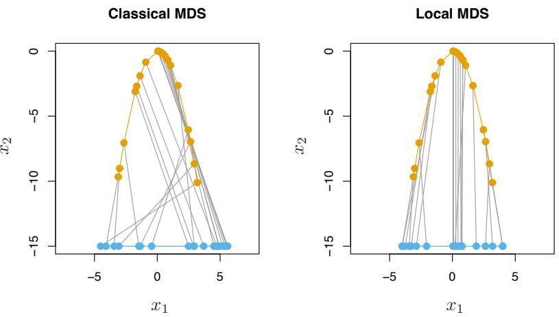
FIGURE 14.44. The orange points show data lying on a parabola, while the blue points shows multidimensional scaling representations in one dimension. Classical multidimensional scaling (left panel) does not preserve the ordering of the points along the curve, because it judges points on opposite ends of the curve to be close together. In contrast, local multidimensional scaling (right panel) does a good job of preserving the ordering of the points along the curve.

serve the ordering of the points along the curve, because it judges points on opposite ends of the curve to be close together. The right panel shows the results of local multi-dimensional scaling, one of the three methods for non-linear multi-dimensional scaling that we discuss below. These methods use only the coordinates of the points in p dimensions, and have no other information about the manifold. Local MDS has done a good job of preserving the ordering of the points along the curve.

We now briefly describe three new approaches to nonlinear dimension reduction and manifold mapping.

Isometric feature mapping (ISOMAP) (Tenenbaum et al., 2000) constructs a graph to approximate the geodesic distance between points along the manifold. Specifically, for each data point we find its neighbors—points within some small Euclidean distance of that point. We construct a graph with an edge between any two neighboring points. The geodesic distance between any two points is then approximated by the shortest path between points on the graph. Finally, classical scaling is applied to the graph distances, to produce a low-dimensional mapping.

Local linear embedding (Roweis and Saul, 2000) takes a very different approach, trying to preserve the local affine structure of the high-dimensional data. Each data point is approximated by a linear combination of neighboring points. Then a lower dimensional representation is constructed that

574 14. Unsupervised Learning

best preserves these local approximations. The details are interesting, so we give them here.

• 1. For each data point xⁱ in p dimensions, we find its K-nearest neighbors N (i) in Euclidean distance.
• 2. We approximate each point by an affine mixture of the points in its neighborhood:

\[\min\_{W\_{ik}} ||x\_i - \sum\_{k \in \mathcal{N}(i)} w\_{ik} x\_k||^2 \tag{14.102}\]

over weights ^wik satisfying ^wik = 0,k/^{∈ N} (i), #^{N k}=1 wik = 1. wik is the contribution of point k to the reconstruction of point i. Note that for a hope of a unique solution, we must have K<p.

3. Finally, we find points yⁱ in a space of dimension d<p to minimize

\[\sum\_{i=1}^{N} ||y\_i - \sum\_{k=1}^{N} w\_{ik} y\_k||^2 \tag{14.103}\]

with wik fixed.

In step 3, we minimize

\[\operatorname{tr}[(\mathbf{Y} - \mathbf{W}\mathbf{Y})^T(\mathbf{Y} - \mathbf{W}\mathbf{Y})] = \operatorname{tr}[\mathbf{Y}^T(\mathbf{I} - \mathbf{W})^T(\mathbf{I} - \mathbf{W})\mathbf{Y}] \tag{14.104}\]

where ^W is ^{N × N}; ^Y is ^{N × d}, for some small d<p. The solutions ^Yˆ are the trailing eigenvectors of ^M = (^{I − W})^T (^{I − W}). Since ¹ is a trivial eigenvector with eigenvalue 0, we discard it and keep the next d. This has the side effect that 1^T Y = 0, and hence the embedding coordinates are mean centered.

Local MDS (Chen and Buja, 2008) takes the simplest and arguably the most direct approach. We define N to be the symmetric set of nearby pairs of points; specifically a pair (i, i′ ) is in N if point i is among the K-nearest neighbors of i ′ , or vice-versa. Then we construct the stress function

\[\begin{split} \left( S\_L(z\_1, z\_2, \dots, z\_N) \right)^2 &= \sum\_{\{i, i'\} \in \mathcal{N}} \left( d\_{ii'} - ||z\_i - z\_{i'}|| \right)^2 \\ &+ \sum\_{\{i, i'\} \notin \mathcal{N}} w \cdot \left( D - ||z\_i - z\_{i'}|| \right)^2. \end{split} \tag{14.105}\]

Here D is some large constant and w is a weight. The idea is that points that are not neighbors are considered to be very far apart; such pairs are given a small weight w so that they don’t dominate the overall stress function. To simplify the expression, we take w ∼ 1/D, and let D → ∞. Expanding (14.105), this gives

FIGURE 14.45. Images of faces mapped into the embedding space described by the first two coordinates of LLE. Next to the circled points, representative faces are shown in different parts of the space. The images at the bottom of the plot correspond to points along the top right path (linked by solid line), and illustrate one particular mode of variability in pose and expression.

576 14. Unsupervised Learning

\[S\_L(z\_1, z\_2, \dots, z\_N) = \sum\_{(i, i') \in \mathcal{N}} (d\_{ii'} - ||z\_i - z\_{i'}||)^2 - \tau \sum\_{(i, i') \notin \mathcal{N}} ||z\_i - z\_{i'}||,\tag{14.106}\]

where τ = 2wD. The first term in (14.106) tries to preserve local structure in the data, while the second term encourages the representations zi, zi′ for pairs (i, i′ ) that are non-neighbors to be farther apart. Local MDS minimizes the stress function (14.106) over zi, for fixed values of the number of neighbors K and the tuning parameter τ .

The right panel of Figure 14.44 shows the result of local MDS, using k = 2 neighbors and τ = 0.01. We used coordinate descent with multiple starting values to find a good minimum of the (nonconvex) stress function (14.106). The ordering of the points along the curve has been largely preserved,

Figure 14.45 shows a more interesting application of one of these methods (LLE)15. The data consist of 1965 photographs, digitized as 20 ^{× 28} grayscale images. The result of the first two-coordinates of LLE are shown and reveal some variability in pose and expression. Similar pictures were produced by local MDS.

In experiments reported in Chen and Buja (2008), local MDS shows superior performance, as compared to ISOMAP and LLE. They also demonstrate the usefulness of local MDS for graph layout. There are also close connections between the methods discussed here, spectral clustering (Section 14.5.3) and kernel PCA (Section 14.5.4).

14.10 The Google PageRank Algorithm

In this section we give a brief description of the original PageRank algorithm used by the Google search engine, an interesting recent application of unsupervised learning methods.

We suppose that we have N web pages and wish to rank them in terms of importance. For example, the N pages might all contain a string match to “statistical learning” and we might wish to rank the pages in terms of their likely relevance to a websurfer.

The PageRank algorithm considers a webpage to be important if many other webpages point to it. However the linking webpages that point to a given page are not treated equally: the algorithm also takes into account both the importance (PageRank) of the linking pages and the number of outgoing links that they have. Linking pages with higher PageRank are given more weight, while pages with more outgoing links are given less weight. These ideas lead to a recursive definition for PageRank, detailed next.

¹⁵Sam Roweis and Lawrence Saul kindly provided this figure.

Let Lij = 1 if page j points to page i, and zero otherwise. Let c^j = #^{N i}=1 Lij equal the number of pages pointed to by page j (number of outlinks). Then the Google PageRanks pⁱ are defined by the recursive relationship

\[p\_i = (1 - d) + d \sum\_{j=1}^{N} (\frac{L\_{ij}}{c\_j}) p\_j \tag{14.107}\]

where d is a positive constant (apparently set to 0.85).

The idea is that the importance of page i is the sum of the importances of pages that point to that page. The sums are weighted by 1/c^j , that is, each page distributes a total vote of 1 to other pages. The constant d ensures that each page gets a PageRank of at least 1 − d. In matrix notation

\[\mathbf{p} = (1 - d)\mathbf{e} + d \cdot \mathbf{L} \mathbf{D}\_c^{-1} \mathbf{p} \tag{14.108}\]

where e is a vector of N ones and D^c = diag(c) is a diagonal matrix with diagonal elements c^j . Introducing the normalization e^T p = N (i.e., the average PageRank is 1), we can write (14.108) as

\[\begin{array}{rcl} \mathbf{p} &=& \left[ (1-d)\mathbf{e} \mathbf{e}^T / N + d \mathbf{L} \mathbf{D}\_c^{-1} \right] \mathbf{p} \\ &=& \mathbf{A} \mathbf{p} \end{array} \tag{14.109}\]

where the matrix A is the expression in square braces.

Exploiting a connection with Markov chains (see below), it can be shown that the matrix A has a real eigenvalue equal to one, and one is its largest eigenvalue. This means that we can find pˆ by the power method: starting with some p = p⁰ we iterate

\[\mathbf{p}\_k \leftarrow \mathbf{A} \mathbf{p}\_{k-1}; \quad \mathbf{p}\_k \leftarrow N \frac{\mathbf{p}\_k}{\mathbf{e}^T \mathbf{p}\_k}. \tag{14.110}\]

The fixed points pˆ are the desired PageRanks.

In the original paper of Page et al. (1998), the authors considered PageRank as a model of user behavior, where a random web surfer clicks on links at random, without regard to content. The surfer does a random walk on the web, choosing among available outgoing links at random. The factor 1 − d is the probability that he does not click on a link, but jumps instead to a random webpage.

Some descriptions of PageRank have (1 − d)/N as the first term in definition (14.107), which would better coincide with the random surfer interpretation. Then the page rank solution (divided by N) is the stationary distribution of an irreducible, aperiodic Markov chain over the N webpages.

Definition (14.107) also corresponds to an irreducible, aperiodic Markov chain, with different transition probabilities than those from he (1 − d)/N version. Viewing PageRank as a Markov chain makes clear why the matrix A has a maximal real eigenvalue of 1. Since A has positive entries with

578 14. Unsupervised Learning

FIGURE 14.46. PageRank algorithm: example of a small network

each column summing to one, Markov chain theory tells us that it has a unique eigenvector with eigenvalue one, corresponding to the stationary distribution of the chain (Bremaud, 1999).

A small network is shown for illustration in Figure 14.46. The link matrix is

\[\mathbf{L} = \begin{pmatrix} 0 & 0 & 1 & 0 \\ 1 & 0 & 0 & 0 \\ 1 & 1 & 0 & 1 \\ 0 & 0 & 0 & 0 \end{pmatrix} \tag{14.111}\]

and the number of outlinks is c = (2, 1, 1, 1).

The PageRank solution is pˆ = (1.49, 0.78, 1.58, 0.15). Notice that page 4 has no incoming links, and hence gets the minimum PageRank of 0.15.

Bibliographic Notes

There are many books on clustering, including Hartigan (1975), Gordon (1999) and Kaufman and Rousseeuw (1990). K-means clustering goes back at least to Lloyd (1957), Forgy (1965), Jancey (1966) and MacQueen (1967). Applications in engineering, especially in image compression via vector quantization, can be found in Gersho and Gray (1992). The k-medoid procedure is described in Kaufman and Rousseeuw (1990). Association rules are outlined in Agrawal et al. (1995). The self-organizing map was proposed by Kohonen (1989) and Kohonen (1990); Kohonen et al. (2000) give a more recent account. Principal components analysis and multidimensional scaling are described in standard books on multivariate analysis, for example, Mardia et al. (1979). Buja et al. (2008) have implemented a powerful environment called Ggvis for multidimensional scaling, and the user manual contains a lucid overview of the subject. Figures 14.17, 14.21 (left panel) and 14.28 (left panel) were produced in Xgobi, a multidimensional data visualization package by the same authors. GGobi is a more recent implementation (Cook and Swayne, 2007). Goodall (1991) gives a technical overview of Procrustes methods in statistics, and Ramsay and Silverman (1997) discuss the shape registration problem. Principal curves and surfaces were proposed in Hastie (1984) and Hastie and Stuetzle (1989). The idea of principal points was formulated in Flury (1990), Tarpey and Flury (1996) give an exposition of the general concept of self-consistency. An excellent tutorial on spectral clustering can be found in von Luxburg (2007); this was the main source for Section 14.5.3. Luxborg credits Donath and Hoffman (1973) and Fiedler (1973) with the earliest work on the subject. A history of spectral clustering my be found in Spielman and Teng (1996). Independent component analysis was proposed by Comon (1994), with subsequent developments by Bell and Sejnowski (1995); our treatment in Section 14.7 is based on Hyv¨arinen and Oja (2000). Projection pursuit was proposed by Friedman and Tukey (1974), and is discussed in detail in Huber (1985). A dynamic projection pursuit algorithm is implemented in GGobi.

Exercises

Ex. 14.1 Weights for clustering. Show that weighted Euclidean distance

\[d\_e^{(w)}(x\_i, x\_{i'}) = \frac{\sum\_{l=1}^p w\_l (x\_{il} - x\_{i'l})^2}{\sum\_{l=1}^p w\_l}\]

satisfies

\[d\_e^{(w)}(x\_i, x\_{i'}) = d\_e(z\_i, z\_{i'}) = \sum\_{l=1}^p (z\_{il} - z\_{i'l})^2,\tag{14.112}\]

where

\[z\_{il} = x\_{il} \cdot \left(\frac{w\_l}{\sum\_{l=1}^p w\_l}\right)^{1/2}.\tag{14.113}\]

Thus weighted Euclidean distance based on x is equivalent to unweighted Euclidean distance based on z.

Ex. 14.2 Consider a mixture model density in p-dimensional feature space,

\[g(x) = \sum\_{k=1}^{K} \pi\_k g\_k(x),\tag{14.114}\]

where ^{gk = N}(µk,L·σ2) and ^{πk ≥ 0 ∀k} with # ^k π^k = 1. Here {µk, πk}, k = 1,…,K and σ² are unknown parameters.

580 14. Unsupervised Learning

Suppose we have data x1, x2,…,x^N ∼ g(x) and we wish to fit the mixture model.

• 1. Write down the log-likelihood of the data
• 2. Derive an EM algorithm for computing the maximum likelihood estimates (see Section 8.1).
• 3. Show that if σ has a known value in the mixture model and we take σ → 0, then in a sense this EM algorithm coincides with K-means clustering.

Ex. 14.3 In Section 14.2.6 we discuss the use of CART or PRIM for constructing generalized association rules. Show that a problem occurs with either of these methods when we generate the random data from the productmarginal distribution; i.e., by randomly permuting the values for each of the variables. Propose ways to overcome this problem.

Ex. 14.4 Cluster the demographic data of Table 14.1 using a classification tree. Specifically, generate a reference sample of the same size of the training set, by randomly permuting the values within each feature. Build a classification tree to the training sample (class 1) and the reference sample (class 0) and describe the terminal nodes having highest estimated class 1 probability. Compare the results to the PRIM results near Table 14.1 and also to the results of K-means clustering applied to the same data.

Ex. 14.5 Generate data with three features, with 30 data points in each of three classes as follows:

\[\begin{array}{rcl} \theta\_1 &=& U(-\pi/8, \pi/8) \\ \phi\_1 &=& U(0, 2\pi) \\ x\_1 &=& \sin(\theta\_1)\cos(\phi\_1) + W\_{11} \\ y\_1 &=& \sin(\theta\_1)\sin(\phi\_1) + W\_{12} \\ z\_1 &=& \cos(\theta\_1) + W\_{13} \\\\ \theta\_2 &=& U(\pi/2 - \pi/4, \pi/2 + \pi/4) \\ \phi\_2 &=& U(-\pi/4, \pi/4) \\ x\_2 &=& \sin(\theta\_2)\cos(\phi\_2) + W\_{21} \\ y\_2 &=& \sin(\theta\_2)\sin(\phi\_2) + W\_{22} \\ z\_2 &=& \cos(\theta\_2) + W\_{23} \\ \end{array}\]

\[\begin{array}{rcl} \theta\_3 &=& U(\pi/2 - \pi/4, \pi/2 + \pi/4) \\ \phi\_3 &=& U(\pi/2 - \pi/4, \pi/2 + \pi/4) \\ x\_3 &=& \sin(\theta\_3)\cos(\phi\_3) + W\_{31} \\ y\_3 &=& \sin(\theta\_3)\sin(\phi\_3) + W\_{32} \\ z\_3 &=& \cos(\theta\_3) + W\_{33} \\ \end{array}\]

Here U(a, b) indicates a uniform variate on the range [a, b] and Wjk are independent normal variates with standard deviation 0.6. Hence the data lie near the surface of a sphere in three clusters centered at (1, 0, 0), (0, 1, 0) and (0, 0, 1).

Write a program to fit a SOM to these data, using the learning rates given in the text. Carry out a K-means clustering of the same data, and compare the results to those in the text.

Ex. 14.6 Write programs to implement K-means clustering and a selforganizing map (SOM), with the prototype lying on a two-dimensional grid. Apply them to the columns of the human tumor microarray data, using K = 2, 5, 10, 20 centroids for both. Demonstrate that as the size of the SOM neighborhood is taken to be smaller and smaller, the SOM solution becomes more similar to the K-means solution.

Ex. 14.7 Derive (14.51) and (14.52) in Section 14.5.1. Show that ˆµ is not unique, and characterize the family of equivalent solutions.

Ex. 14.8 Derive the solution (14.57) to the Procrustes problem (14.56). Derive also the solution to the Procrustes problem with scaling (14.58).

Ex. 14.9 Write an algorithm to solve

\[\min\_{\{\beta\_{\ell}, \mathbf{R}\_{\ell}\}\_{1}^{L}, \mathbf{M}} \sum\_{\ell=1}^{L} ||\mathbf{X}\_{\ell} \mathbf{R}\_{\ell} - \mathbf{M}||\_{F}^{2}. \tag{14.115}\]

Apply it to the three S’s, and compare the results to those shown in Figure 14.26.

Ex. 14.10 Derive the solution to the affine-invariant average problem (14.60). Apply it to the three S’s, and compare the results to those computed in Exercise 14.9.

Ex. 14.11 Classical multidimensional scaling. Let S be the centered inner product matrix with elements ⟨xⁱ − x, x ¯ ^j − x¯⟩. Let λ¹ > λ² > ··· > λ^k be the k largest eigenvalues of S, with associated eigenvectors E^k = (e1, ^e2,…, ^ek). Let ^Dk be a diagonal matrix with diagonal entries ^√λ1, ^√λ2, …, ^√λk. Show that the solutions ^zi to the classical scaling problem (14.100) are the rows of EkDk.

Ex. 14.12 Consider the sparse PCA criterion (14.71).

• 1. Show that with Θ fixed, solving for V amounts to K separate elasticnet regression problems, with responses the K elements of Θ^T xi.
• 2. Show that with V fixed, solving for Θ amounts to a reduced-rank version of the Procrustes problem, which reduces to

\[\max\_{\boldsymbol{\Theta}} \text{trace}(\boldsymbol{\Theta}^T \mathbf{M}) \text{ subject to } \boldsymbol{\Theta}^T \boldsymbol{\Theta} = \mathbf{I}\_K,\tag{14.116}\]

where ^M and ^Θ are both ^{p × K} with ^{K ≤ p}. If ^{M =} UDQ^T is the SVD of M, show that the optimal Θ = UQ^T .

582 14. Unsupervised Learning

Ex. 14.13 Generate 200 data points with three features, lying close to a helix. In detail, define X¹ = cos(s)+0.1 · Z1, X² = sin(s)+0.1 · Z2, X³ = s + 0.1 · Z³ where s takes on 200 equally spaced values between 0 and 2π, and Z1, Z2, Z³ are independent and have standard Gaussian distributions.

• 1. Fit a principal curve to the data and plot the estimated coordinate functions. Compare them to the underlying functions cos(s),sin(s) and s.
• 2. Fit a self-organizing map to the same data, and see if you can discover the helical shape of the original point cloud.

Ex. 14.14 Pre- and post-multiply equation (14.81) by a diagonal matrix containing the inverse variances of the X^j . Hence obtain an equivalent decomposition for the correlation matrix, in the sense that a simple scaling is applied to the matrix A.

Ex. 14.15 Generate 200 observations of three variates X1, X2, X³ according to

\[\begin{array}{rcl} X\_1 & \sim & Z\_1\\ X\_2 & = & X\_1 + 0.001 \cdot Z\_2\\ X\_3 & = & 10 \cdot Z\_3 \end{array} \tag{14.117}\]

where Z1, Z2, Z³ are independent standard normal variates. Compute the leading principal component and factor analysis directions. Hence show that the leading principal component aligns itself in the maximal variance direction X3, while the leading factor essentially ignores the uncorrelated component X3, and picks up the correlated component X² + X¹ (Geoffrey Hinton, personal communication).

Ex. 14.16 Consider the kernel principal component procedure outlined in Section 14.5.4. Argue that the number M of principal components is equal to the rank of K, which is the number of non-zero elements in D. Show that the mth component z^m (mth column of Z) can be written (up to centering) as zim = #^{N j}=1 αjmK(xi, x^j ), where αjm = ujm/dm. Show that the mapping of a new observation x⁰ to the mth component is given by z0^m = #^{N j}=1 αjmK(x0, x^j ).

Ex. 14.17 Show that with g1(x) = #^{N j}=1 cjK(x, x^j ), the solution to (14.66) is given by ˆc^j = uj1/d1, where u¹ is the first column of U in (14.65), and d¹ the first diagonal element of D. Show that the second and subsequent principal component functions are defined in a similar manner (hint: see Section 5.8.1.)

Ex. 14.18 Consider the regularized log-likelihood for the density estimation problem arising in ICA,

Exercises 583

\[\frac{1}{N} \sum\_{i=1}^{N} \left[ \log \phi(s\_i) + g(s\_i) \right] - \int \phi(t) e^{g(t)} dt - \lambda \int \{g'''(t)\}^2(t) dt. \tag{14.118}\]

The solution ˆg is a quartic smoothing spline, and can be written as ˆg(s) = qˆ(s)+ˆq⊥(s), where q is a quadratic function (in the null space of the penalty). Let q(s) = θ⁰ + θ1s + θ2s2. By examining the stationarity conditions for ˆθk, k = 1, 2, 3, show that the solution ˆf = φeg^ˆ is a density, and has mean zero and variance one. If we used a second-derivative penalty 5 {g′′(t)}2(t)dt instead, what simple modification could we make to the problem to maintain the three moment conditions?

Ex. 14.19 If A is p × p orthogonal, show that the first term in (14.92) on page 568

\[\sum\_{j=1}^{p} \sum\_{i=1}^{N} \log \phi(a\_j^T x\_i),\]

with a^j the jth column of A, does not depend on A.

Ex. 14.20 Fixed point algorithm for ICA (Hyv¨arinen et al., 2001). Consider maximizing ^C(a) = ^E{g(a^{T X})} with respect to ^a, with ||a|| = 1 and Cov(X) = I. Use a Lagrange multiplier to enforce the norm constraint, and write down the first two derivatives of the modified criterion. Use the approximation

\[\mathbb{E}\{XX^T g''(a^T X)\} \approx \mathbb{E}\{XX^T\} \mathbb{E}\{g''(a^T X)\}\]

to show that the Newton update can be written as the fixed-point update (14.96).

Ex. 14.21 Consider an undirected graph with non-negative edge weights wii′ and graph Laplacian L. Suppose there are m connected components A1, A2,…,A^m in the graph. Show that there are m eigenvectors of L corresponding to eigenvalue zero, and the indicator vectors of these components I^A1 , I^A2 ,…,I^Am span the zero eigenspace.

Ex. 14.22

• 1. Show that definition (14.108) implies that the sum of the PageRanks pⁱ is N, the number of web pages.
• 2. Write a program to compute the PageRank solutions by the power method using formulation (14.107). Apply it to the network of Figure 14.47.

Ex. 14.23 Algorithm for non-negative matrix factorization (Wu and Lange, 2007). A function g(x, y) to said to minorize a function f(x) if

584 14. Unsupervised Learning

FIGURE 14.47. Example of a small network.

\[g(x, y) \le f(x), \ g(x, x) = f(x) \tag{14.119}\]

for all x, y in the domain. This is useful for maximizing f(x) since it is easy to show that f(x) is nondecreasing under the update

\[x^{s+1} = \operatorname\*{argmax}\_{x} g(x, x^s) \tag{14.120}\]

There are analogous definitions for majorization, for minimizing a function f(x). The resulting algorithms are known as MM algorithms, for “minorizemaximize” or “majorize-minimize” (Lange, 2004). It also can be shown that the EM algorithm (8.5) is an example of an MM algorithm: see Section 8.5.3 and Exercise 8.2 for details.

1. Consider maximization of the function L(W, H) in (14.73), written here without the matrix notation

\[L(\mathbf{W}, \mathbf{H}) = \sum\_{i=1}^{N} \sum\_{j=1}^{p} \left[ x\_{ij} \log \left( \sum\_{k=1}^{r} w\_{ik} h\_{kj} \right) - \sum\_{k=1}^{r} w\_{ik} h\_{kj} \right].\]

Using the concavity of log(x), show that for any set of r values y^k ≥ 0 and 0 ^{≤ ck ≤} 1 with #^{r k}=1 c^k = 1,

\[\log\left(\sum\_{k=1}^r y\_k\right) \ge \sum\_{k=1}^r c\_k \log(y\_k/c\_k)\]

Hence

\[\log\left(\sum\_{k=1}^r w\_{ik} h\_{kj}\right) \ge \sum\_{k=1}^r \frac{a\_{ikj}^s}{b\_{ij}^s} \log\left(\frac{b\_{ij}^s}{a\_{ikj}^s} w\_{ik} h\_{kj}\right),\]

where

\[a\_{ikj}^s = w\_{ik}^s h\_{kj}^s \text{ and } b\_{ij}^s = \sum\_{k=1}^r w\_{ik}^s h\_{kj}^s,\]

and s indicates the current iteration.

2. Hence show that, ignoring constants, the function

\[\begin{aligned} g(\mathbf{W}, \mathbf{H} \mid \mathbf{W}^s, \mathbf{H}^s) &= \sum\_{i=1}^N \sum\_{j=1}^p \sum\_{k=1}^r u\_{ij} \frac{a\_{ikj}^s}{b\_{ij}^s} \left( \log w\_{ik} + \log h\_{kj} \right) \\ &- \sum\_{i=1}^N \sum\_{j=1}^p \sum\_{k=1}^r w\_{ik} h\_{kj} \end{aligned}\]

minorizes L(W, H).

3. Set the partial derivatives of ^g(W, ^{H | W}s, ^Hs) to zero and hence derive the updating steps (14.74).

Ex. 14.24 Consider the non-negative matrix factorization (14.72) in the rank one case (r = 1).

1. Show that the updates (14.74) reduce to

\[\begin{aligned} w\_i &\leftarrow w\_i \frac{\sum\_{j=1}^p x\_{ij}}{\sum\_{j=1}^p w\_i h\_j} \\ h\_j &\leftarrow h\_j \frac{\sum\_{i=1}^N x\_{ij}}{\sum\_{i=1}^N w\_i h\_j} \end{aligned} \tag{14.121}\]

where wⁱ = wi1, h^j = h1^j . This is an example of the iterative proportional scaling procedure, applied to the independence model for a two-way contingency table (Fienberg, 1977, for example).

2. Show that the final iterates have the explicit form

\[w\_i = c \cdot \frac{\sum\_{j=1}^{p} x\_{ij}}{\sum\_{i=1}^{N} \sum\_{j=1}^{p} x\_{ij}}, \quad h\_k = \frac{1}{c} \cdot \frac{\sum\_{i=1}^{N} x\_{ik}}{\sum\_{i=1}^{N} \sum\_{j=1}^{p} x\_{ij}} \tag{14.122}\]

for any constant c > 0. These are equivalent to the usual row and column estimates for a two-way independence model.

Ex. 14.25 Fit a non-negative matrix factorization model to the collection of two’s in the digits database. Use 25 basis elements, and compare with a 24- component (plus mean) PCA model. In both cases display the W and H matrices as in Figure 14.33.

586 14. Unsupervised Learning

This is page 587 Printer: Opaque this

15 Random Forests

15.1 Introduction

Bagging or bootstrap aggregation (section 8.7) is a technique for reducing the variance of an estimated prediction function. Bagging seems to work especially well for high-variance, low-bias procedures, such as trees. For regression, we simply fit the same regression tree many times to bootstrapsampled versions of the training data, and average the result. For classification, a committee of trees each cast a vote for the predicted class.

Boosting in Chapter 10 was initially proposed as a committee method as well, although unlike bagging, the committee of weak learners evolves over time, and the members cast a weighted vote. Boosting appears to dominate bagging on most problems, and became the preferred choice.

Random forests (Breiman, 2001) is a substantial modification of bagging that builds a large collection of de-correlated trees, and then averages them. On many problems the performance of random forests is very similar to boosting, and they are simpler to train and tune. As a consequence, random forests are popular, and are implemented in a variety of packages.

15.2 Definition of Random Forests

The essential idea in bagging (Section 8.7) is to average many noisy but approximately unbiased models, and hence reduce the variance. Trees are ideal candidates for bagging, since they can capture complex interaction Algorithm 15.1 Random Forest for Regression or Classification.

1. For b = 1 to B:

• 1. Draw a bootstrap sample Z^∗ of size N from the training data.
• 2. Grow a random-forest tree T^b to the bootstrapped data, by recursively repeating the following steps for each terminal node of the tree, until the minimum node size nmin is reached.
  • 1. Select m variables at random from the p variables.
  • 2. Pick the best variable/split-point among the m.
  • 3. Split the node into two daughter nodes.
• 2. Output the ensemble of trees {Tb}^B 1 .

To make a prediction at a new point x:

Regression: ˆf ^B rf (x) = ¹ B #^{B b}=1 Tb(x).

Classification: Let Cˆb(x) be the class prediction of the bth random-forest tree. Then Cˆ^B rf (x) = majority vote {Cˆb(x)}^B 1 .

structures in the data, and if grown sufficiently deep, have relatively low bias. Since trees are notoriously noisy, they benefit greatly from the averaging. Moreover, since each tree generated in bagging is identically distributed (i.d.), the expectation of an average of B such trees is the same as the expectation of any one of them. This means the bias of bagged trees is the same as that of the individual trees, and the only hope of improvement is through variance reduction. This is in contrast to boosting, where the trees are grown in an adaptive way to remove bias, and hence are not i.d.

An average of B i.i.d. random variables, each with variance σ², has variance ^{1 B} σ². If the variables are simply i.d. (identically distributed, but not necessarily independent) with positive pairwise correlation ρ, the variance of the average is (Exercise 15.1)

\[ \rho \sigma^2 + \frac{1-\rho}{B} \sigma^2. \tag{15.1} \]

As B increases, the second term disappears, but the first remains, and hence the size of the correlation of pairs of bagged trees limits the benefits of averaging. The idea in random forests (Algorithm 15.1) is to improve the variance reduction of bagging by reducing the correlation between the trees, without increasing the variance too much. This is achieved in the tree-growing process through random selection of the input variables.

Specifically, when growing a tree on a bootstrapped dataset:

Before each split, select m ≤ p of the input variables at random as candidates for splitting.

Typically values for m are √p or even as low as 1.

After ^B such trees {T(x; ^Θb)}^{B 1} are grown, the random forest (regression) predictor is

\[\hat{f}\_{\rm rf}^{B}(x) = \frac{1}{B} \sum\_{b=1}^{B} T(x; \Theta\_b). \tag{15.2}\]

As in Section 10.9 (page 356), Θ^b characterizes the bth random forest tree in terms of split variables, cutpoints at each node, and terminal-node values. Intuitively, reducing m will reduce the correlation between any pair of trees in the ensemble, and hence by (15.1) reduce the variance of the average.

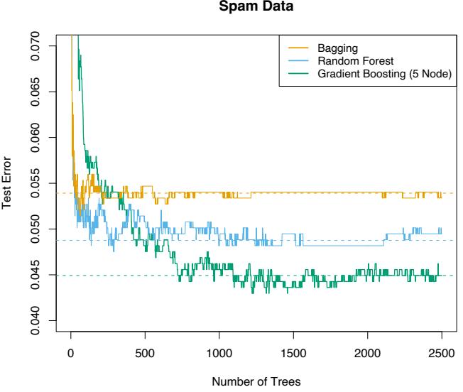
FIGURE 15.1. Bagging, random forest, and gradient boosting, applied to the spam data. For boosting, 5-node trees were used, and the number of trees were chosen by 10-fold cross-validation (2500 trees). Each “step” in the figure corresponds to a change in a single misclassification (in a test set of 1536).

Not all estimators can be improved by shaking up the data like this. It seems that highly nonlinear estimators, such as trees, benefit the most. For bootstrapped trees, ρ is typically small (0.05 or lower is typical; see Figure 15.9), while σ² is not much larger than the variance for the original tree. On the other hand, bagging does not change linear estimates, such as the sample mean (hence its variance either); the pairwise correlation between bootstrapped means is about 50% (Exercise 15.4).

590 15. Random Forests

Random forests are popular. Leo Breiman’s¹ collaborator Adele Cutler maintains a random forest website² where the software is freely available, with more than 3000 downloads reported by 2002. There is a randomForest package in R, maintained by Andy Liaw, available from the CRAN website.

The authors make grand claims about the success of random forests: “most accurate,” “most interpretable,” and the like. In our experience random forests do remarkably well, with very little tuning required. A random forest classifier achieves 4.88% misclassification error on the spam test data, which compares well with all other methods, and is not significantly worse than gradient boosting at 4.5%. Bagging achieves 5.4% which is significantly worse than either (using the McNemar test outlined in Exercise 10.6), so it appears on this example the additional randomization helps.

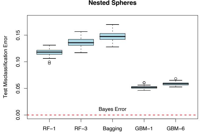
FIGURE 15.2. The results of 50 simulations from the “nested spheres” model in IR¹⁰. The Bayes decision boundary is the surface of a sphere (additive). “RF-3” refers to a random forest with m = 3, and “GBM-6” a gradient boosted model with interaction order six; similarly for “RF-1” and “GBM-1.” The training sets were of size 2000, and the test sets 10, 000.

Figure 15.1 shows the test-error progression on 2500 trees for the three methods. In this case there is some evidence that gradient boosting has started to overfit, although 10-fold cross-validation chose all 2500 trees.

¹Sadly, Leo Breiman died in July, 2005.

²http://www.math.usu.edu/∼adele/forests/

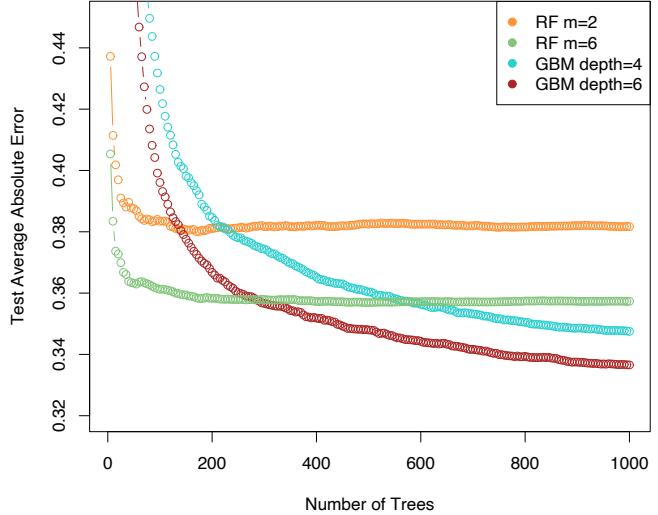
California Housing Data

FIGURE 15.3. Random forests compared to gradient boosting on the California housing data. The curves represent mean absolute error on the test data as a function of the number of trees in the models. Two random forests are shown, with m = 2 and m = 6. The two gradient boosted models use a shrinkage parameter ν = 0.05 in (10.41), and have interaction depths of 4 and 6. The boosted models outperform random forests.

Figure 15.2 shows the results of a simulation³ comparing random forests to gradient boosting on the nested spheres problem [Equation (10.2) in Chapter 10]. Boosting easily outperforms random forests here. Notice that smaller m is better here, although part of the reason could be that the true decision boundary is additive.

Figure 15.3 compares random forests to boosting (with shrinkage) in a regression problem, using the California housing data (Section 10.14.1). Two strong features that emerge are

• Random forests stabilize at about 200 trees, while at 1000 trees boosting continues to improve. Boosting is slowed down by the shrinkage, as well as the fact that the trees are much smaller.
• Boosting outperforms random forests here. At 1000 terms, the weaker boosting model (GBM depth 4) has a smaller error than the stronger

³Details: The random forests were fit using the R package randomForest 4.5-11, with 500 trees. The gradient boosting models were fit using R package gbm 1.5, with shrinkage parameter set to 0.05, and 2000 trees.

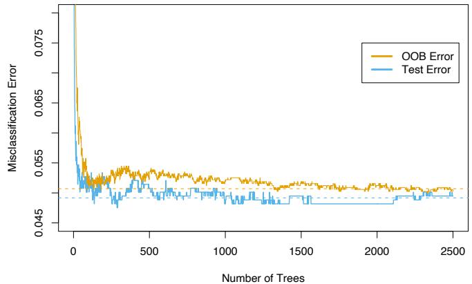
FIGURE 15.4. oob error computed on the spam training data, compared to the test error computed on the test set.

random forest (RF m = 6); a Wilcoxon test on the mean differences in absolute errors has a p-value of 0.007. For larger m the random forests performed no better.

15.3 Details of Random Forests

We have glossed over the distinction between random forests for classification versus regression. When used for classification, a random forest obtains a class vote from each tree, and then classifies using majority vote (see Section 8.7 on bagging for a similar discussion). When used for regression, the predictions from each tree at a target point x are simply averaged, as in (15.2). In addition, the inventors make the following recommendations:

• For classification, the default value for m is ⌊ ^√p⌋ and the minimum node size is one.
• For regression, the default value for m is ⌊p/3⌋ and the minimum node size is five.

In practice the best values for these parameters will depend on the problem, and they should be treated as tuning parameters. In Figure 15.3 the m = 6 performs much better than the default value ⌊8/3⌋ = 2.

15.3.1 Out of Bag Samples

An important feature of random forests is its use of out-of-bag (oob) samples:

For each observation zⁱ = (xi, yi), construct its random forest predictor by averaging only those trees corresponding to bootstrap samples in which zⁱ did not appear.

An oob error estimate is almost identical to that obtained by N-fold crossvalidation; see Exercise 15.2. Hence unlike many other nonlinear estimators, random forests can be fit in one sequence, with cross-validation being performed along the way. Once the oob error stabilizes, the training can be terminated.

Figure 15.4 shows the oob misclassification error for the spam data, compared to the test error. Although 2500 trees are averaged here, it appears from the plot that about 200 would be sufficient.

15.3.2 Variable Importance

Variable importance plots can be constructed for random forests in exactly the same way as they were for gradient-boosted models (Section 10.13). At each split in each tree, the improvement in the split-criterion is the importance measure attributed to the splitting variable, and is accumulated over all the trees in the forest separately for each variable. The left plot of Figure 15.5 shows the variable importances computed in this way for the spam data; compare with the corresponding Figure 10.6 on page 354 for gradient boosting. Boosting ignores some variables completely, while the random forest does not. The candidate split-variable selection increases the chance that any single variable gets included in a random forest, while no such selection occurs with boosting.

Random forests also use the oob samples to construct a different variableimportance measure, apparently to measure the prediction strength of each variable. When the bth tree is grown, the oob samples are passed down the tree, and the prediction accuracy is recorded. Then the values for the jth variable are randomly permuted in the oob samples, and the accuracy is again computed. The decrease in accuracy as a result of this permuting is averaged over all trees, and is used as a measure of the importance of variable j in the random forest. These are expressed as a percent of the maximum in the right plot in Figure 15.5. Although the rankings of the two methods are similar, the importances in the right plot are more uniform over the variables. The randomization effectively voids the effect of a variable, much like setting a coefficient to zero in a linear model (Exercise 15.7). This does not measure the effect on prediction were this variable not available, because if the model was refitted without the variable, other variables could be used as surrogates.

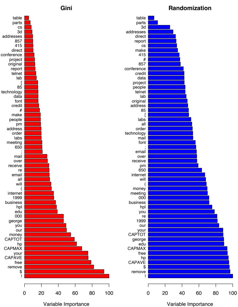
FIGURE 15.5. Variable importance plots for a classification random forest grown on the spam data. The left plot bases the importance on the Gini splitting index, as in gradient boosting. The rankings compare well with the rankings produced by gradient boosting (Figure 10.6 on page 354). The right plot uses oob randomization to compute variable importances, and tends to spread the importances more uniformly.

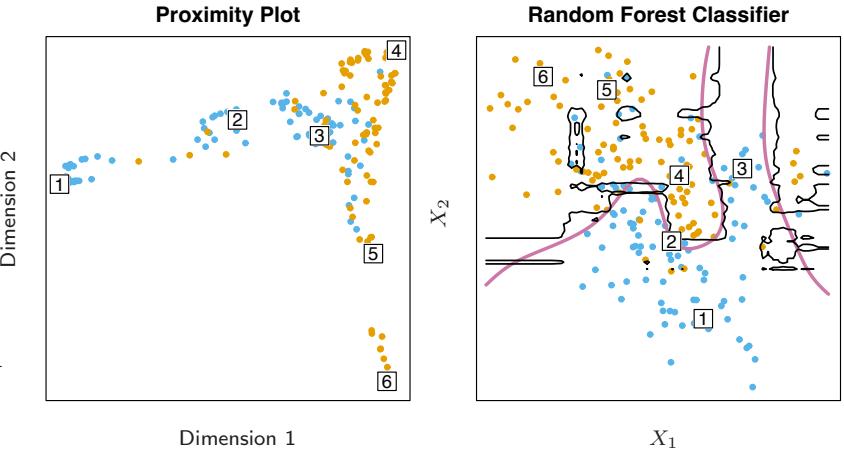
FIGURE 15.6. (Left): Proximity plot for a random forest classifier grown to the mixture data. (Right): Decision boundary and training data for random forest on mixture data. Six points have been identified in each plot.

15.3.3 Proximity Plots

One of the advertised outputs of a random forest is a proximity plot. Figure 15.6 shows a proximity plot for the mixture data defined in Section 2.3.3 in Chapter 2. In growing a random forest, an N × N proximity matrix is accumulated for the training data. For every tree, any pair of oob observations sharing a terminal node has their proximity increased by one. This proximity matrix is then represented in two dimensions using multidimensional scaling (Section 14.8). The idea is that even though the data may be high-dimensional, involving mixed variables, etc., the proximity plot gives an indication of which observations are effectively close together in the eyes of the random forest classifier.

Proximity plots for random forests often look very similar, irrespective of the data, which casts doubt on their utility. They tend to have a star shape, one arm per class, which is more pronounced the better the classification performance.

Since the mixture data are two-dimensional, we can map points from the proximity plot to the original coordinates, and get a better understanding of what they represent. It seems that points in pure regions class-wise map to the extremities of the star, while points nearer the decision boundaries map nearer the center. This is not surprising when we consider the construction of the proximity matrices. Neighboring points in pure regions will often end up sharing a bucket, since when a terminal node is pure, it is no longer split by a random forest tree-growing algorithm. On the other hand, pairs of points that are close but belong to different classes will sometimes share a terminal node, but not always.

15.3.4 Random Forests and Overfitting

When the number of variables is large, but the fraction of relevant variables small, random forests are likely to perform poorly with small m. At each split the chance can be small that the relevant variables will be selected. Figure 15.7 shows the results of a simulation that supports this claim. Details are given in the figure caption and Exercise 15.3. At the top of each pair we see the hyper-geometric probability that a relevant variable will be selected at any split by a random forest tree (in this simulation, the relevant variables are all equal in stature). As this probability gets small, the gap between boosting and random forests increases. When the number of relevant variables increases, the performance of random forests is surprisingly robust to an increase in the number of noise variables. For example, with 6 relevant and 100 noise variables, the probability of a relevant variable being selected at any split is 0.46, assuming ^{m = O}(6 + 100) ^≈ 10. According to Figure 15.7, this does not hurt the performance of random forests compared with boosting. This robustness is largely due to the relative insensitivity of misclassification cost to the bias and variance of the probability estimates in each tree. We consider random forests for regression in the next section.

Another claim is that random forests “cannot overfit” the data. It is certainly true that increasing B does not cause the random forest sequence to overfit; like bagging, the random forest estimate (15.2) approximates the expectation

\[\hat{f}\_{\rm rf}(x) = \mathcal{E}\_{\Theta} T(x; \Theta) = \lim\_{B \to \infty} \hat{f}(x)\_{\rm rf}^{B} \tag{15.3}\]

with an average over B realizations of Θ. The distribution of Θ here is conditional on the training data. However, this limit can overfit the data; the average of fully grown trees can result in too rich a model, and incur unnecessary variance. Segal (2004) demonstrates small gains in performance by controlling the depths of the individual trees grown in random forests. Our experience is that using full-grown trees seldom costs much, and results in one less tuning parameter.

Figure 15.8 shows the modest effect of depth control in a simple regression example. Classifiers are less sensitive to variance, and this effect of overfitting is seldom seen with random-forest classification.

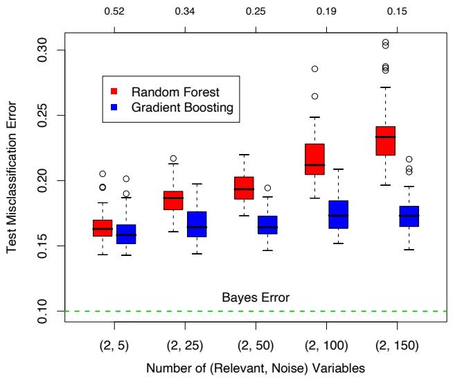
FIGURE 15.7. A comparison of random forests and gradient boosting on problems with increasing numbers of noise variables. In each case the true decision boundary depends on two variables, and an increasing number of noise variables are included. Random forests uses its default value m = √p. At the top of each pair is the probability that one of the relevant variables is chosen at any split. The results are based on 50 simulations for each pair, with a training sample of 300, and a test sample of 500.

15.4 Analysis of Random Forests

In this section we analyze the mechanisms at play with the additional randomization employed by random forests. For this discussion we focus on regression and squared error loss, since this gets at the main points, and bias and variance are more complex with 0–1 loss (see Section 7.3.1). Furthermore, even in the case of a classification problem, we can consider the random-forest average as an estimate of the class posterior probabilities, for which bias and variance are appropriate descriptors.

15.4.1 Variance and the De-Correlation Effect

The limiting form (B → ∞) of the random forest regression estimator is

\[\hat{f}\_{\rm rf}(x) = \mathbf{E}\_{\Theta|\mathbf{Z}} T(x; \Theta(\mathbf{Z})),\tag{15.4}\]

where we have made explicit the dependence on the training data Z. Here we consider estimation at a single target point x. From (15.1) we see that

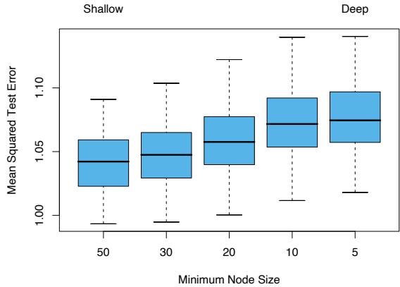
FIGURE 15.8. The effect of tree size on the error in random forest regression. In this example, the true surface was additive in two of the 12 variables, plus additive unit-variance Gaussian noise. Tree depth is controlled here by the minimum node size; the smaller the minimum node size, the deeper the trees.

\[\text{Var}\hat{f}\_{\text{rf}}(x) = \rho(x)\sigma^2(x). \tag{15.5}\]

Here

• ρ(x) is the sampling correlation between any pair of trees used in the averaging:

\[\rho(x) = \text{corr}[T(x; \Theta\_1(\mathbf{Z})), T(x; \Theta\_2(\mathbf{Z}))],\tag{15.6}\]

where Θ1(Z) and Θ2(Z) are a randomly drawn pair of random forest trees grown to the randomly sampled Z;

• ^σ2(x) is the sampling variance of any single randomly drawn tree,

\[ \sigma^2(x) = \text{Var}\, T(x; \Theta(\mathbf{Z})).\tag{15.7} \]

It is easy to confuse ρ(x) with the average correlation between fitted trees in a given random-forest ensemble; that is, think of the fitted trees as Nvectors, and compute the average pairwise correlation between these vectors, conditioned on the data. This is not the case; this conditional correlation is not directly relevant in the averaging process, and the dependence on x in ρ(x) warns us of the distinction. Rather, ρ(x) is the theoretical correlation between a pair of random-forest trees evaluated at x, induced by repeatedly making training sample draws Z from the population, and then drawing a pair of random forest trees. In statistical jargon, this is the correlation induced by the sampling distribution of Z and Θ.

More precisely, the variability averaged over in the calculations in (15.6) and (15.7) is both

• conditional on Z: due to the bootstrap sampling and feature sampling at each split, and
• a result of the sampling variability of Z itself.

In fact, the conditional covariance of a pair of tree fits at x is zero, because the bootstrap and feature sampling is i.i.d; see Exercise 15.5.

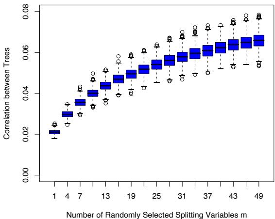
FIGURE 15.9. Correlations between pairs of trees drawn by a random-forest regression algorithm, as a function of m. The boxplots represent the correlations at 600 randomly chosen prediction points x.

The following demonstrations are based on a simulation model

\[Y = \frac{1}{\sqrt{50}} \sum\_{j=1}^{50} X\_j + \varepsilon,\tag{15.8}\]

with all the X^j and ε iid Gaussian. We use 500 training sets of size 100, and a single set of test locations of size 600. Since regression trees are nonlinear in Z, the patterns we see below will differ somewhat depending on the structure of the model.

Figure 15.9 shows how the correlation (15.6) between pairs of trees decreases as m decreases: pairs of tree predictions at x for different training sets Z are likely to be less similar if they do not use the same splitting variables.

In the left panel of Figure 15.10 we consider the variances of single tree predictors, VarT(x; Θ(Z)) (averaged over 600 prediction points x drawn randomly from our simulation model). This is the total variance, and can be

600 15. Random Forests

decomposed into two parts using standard conditional variance arguments (see Exercise 15.5):

\[\begin{array}{rcl} \text{Var}\_{\Theta, \mathbf{Z}} T(x; \Theta(\mathbf{Z})) &=& \text{Var}\_{\mathbf{Z}} \text{E}\_{\Theta|\mathbf{Z}} T(x; \Theta(\mathbf{Z})) &+& \text{E}\_{\mathbf{Z}} \text{Var}\_{\Theta|\mathbf{Z}} T(x; \Theta(\mathbf{Z})) \\\\ \text{Total Variance} &=& \text{Var}\_{\mathbf{Z}} \hat{f}\_{\text{rf}}(x) &+& \text{within-} \mathbf{Z} \text{ Variance} \end{array} \tag{15.9}\]

The second term is the within-Z variance—a result of the randomization, which increases as m decreases. The first term is in fact the sampling variance of the random forest ensemble (shown in the right panel), which decreases as m decreases. The variance of the individual trees does not change appreciably over much of the range of m, hence in light of (15.5), the variance of the ensemble is dramatically lower than this tree variance.

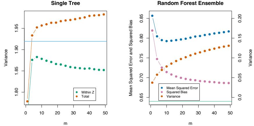
FIGURE 15.10. Simulation results. The left panel shows the average variance of a single random forest tree, as a function of m. “Within Z” refers to the average within-sample contribution to the variance, resulting from the bootstrap sampling and split-variable sampling (15.9). “Total” includes the sampling variability of Z. The horizontal line is the average variance of a single fully grown tree (without bootstrap sampling). The right panel shows the average mean-squared error, squared bias and variance of the ensemble, as a function of m. Note that the variance axis is on the right (same scale, different level). The horizontal line is the average squared-bias of a fully grown tree.

15.4.2 Bias

As in bagging, the bias of a random forest is the same as the bias of any of the individual sampled trees T(x; Θ(Z)):

15.4 Analysis of Random Forests 601

\[\begin{split} \text{Bias}(x) &= \quad \mu(x) - \text{E}\_{\mathbf{Z}} \hat{f}\_{\text{rf}}(x) \\ &= \quad \mu(x) - \text{E}\_{\mathbf{Z}} \text{E}\_{\Theta|\mathbf{Z}} T(x; \Theta(\mathbf{Z})). \end{split} \tag{15.10}\]

This is also typically greater (in absolute terms) than the bias of an unpruned tree grown to Z, since the randomization and reduced sample space impose restrictions. Hence the improvements in prediction obtained by bagging or random forests are solely a result of variance reduction.

Any discussion of bias depends on the unknown true function. Figure 15.10 (right panel) shows the squared bias for our additive model simulation (estimated from the 500 realizations). Although for different models the shape and rate of the bias curves may differ, the general trend is that as m decreases, the bias increases. Shown in the figure is the mean-squared error, and we see a classical bias-variance trade-off in the choice of m. For all m the squared bias of the random forest is greater than that for a single tree (horizontal line).

These patterns suggest a similarity with ridge regression (Section 3.4.1). Ridge regression is useful (in linear models) when one has a large number of variables with similarly sized coefficients; ridge shrinks their coefficients toward zero, and those of strongly correlated variables toward each other. Although the size of the training sample might not permit all the variables to be in the model, this regularization via ridge stabilizes the model and allows all the variables to have their say (albeit diminished). Random forests with small m perform a similar averaging. Each of the relevant variables get their turn to be the primary split, and the ensemble averaging reduces the contribution of any individual variable. Since this simulation example (15.8) is based on a linear model in all the variables, ridge regression achieves a lower mean-squared error (about 0.45 with df(λopt) ≈ 29).

15.4.3 Adaptive Nearest Neighbors

The random forest classifier has much in common with the k-nearest neighbor classifier (Section 13.3); in fact a weighted version thereof. Since each tree is grown to maximal size, for a particular Θ^∗, T(x; Θ^∗(Z)) is the response value for one of the training samples⁴. The tree-growing algorithm finds an “optimal” path to that observation, choosing the most informative predictors from those at its disposal. The averaging process assigns weights to these training responses, which ultimately vote for the prediction. Hence via the random-forest voting mechanism, those observations close to the target point get assigned weights—an equivalent kernel—which combine to form the classification decision.

Figure 15.11 demonstrates the similarity between the decision boundary of 3-nearest neighbors and random forests on the mixture data.

⁴We gloss over the fact that pure nodes are not split further, and hence there can be more than one observation in a terminal node

602 15. Random Forests

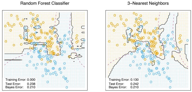
FIGURE 15.11. Random forests versus 3-NN on the mixture data. The axis-oriented nature of the individual trees in a random forest lead to decision regions with an axis-oriented flavor.

Bibliographic Notes

Random forests as described here were introduced by Breiman (2001), although many of the ideas had cropped up earlier in the literature in different forms. Notably Ho (1995) introduced the term “random forest,” and used a consensus of trees grown in random subspaces of the features. The idea of using stochastic perturbation and averaging to avoid overfitting was introduced by Kleinberg (1990), and later in Kleinberg (1996). Amit and Geman (1997) used randomized trees grown on image features for image classification problems. Breiman (1996a) introduced bagging, a precursor to his version of random forests. Dietterich (2000b) also proposed an improvement on bagging using additional randomization. His approach was to rank the top 20 candidate splits at each node, and then select from the list at random. He showed through simulations and real examples that this additional randomization improved over the performance of bagging. Friedman and Hall (2007) showed that sub-sampling (without replacement) is an effective alternative to bagging. They showed that growing and averaging trees on samples of size N/2 is approximately equivalent (in terms bias/variance considerations) to bagging, while using smaller fractions of N reduces the variance even further (through decorrelation).

There are several free software implementations of random forests. In this chapter we used the randomForest package in R, maintained by Andy Liaw, available from the CRAN website. This allows both split-variable selection, as well as sub-sampling. Adele Cutler maintains a random forest website http://www.math.usu.edu/∼adele/forests/ where (as of August 2008) the software written by Leo Breiman and Adele Cutler is freely available. Their code, and the name “random forests”, is exclusively licensed to Salford Systems for commercial release. The Weka machine learning archive http://www.cs.waikato.ac.nz/ml/weka/ at Waikato University, New Zealand, offers a free java implementation of random forests.

Exercises

Ex. 15.1 Derive the variance formula (15.1). This appears to fail if ρ is negative; diagnose the problem in this case.

Ex. 15.2 Show that as the number of bootstrap samples B gets large, the oob error estimate for a random forest approaches its N-fold CV error estimate, and that in the limit, the identity is exact.

Ex. 15.3 Consider the simulation model used in Figure 15.7 (Mease and Wyner, 2008). Binary observations are generated with probabilities

\[\Pr(Y=1|X) = q + (1-2q) \cdot 1 \left[ \sum\_{j=1}^{J} X\_j > J/2 \right],\tag{15.11}\]

where ^{X ∼ U}[0, 1]^p, 0 ^{≤ q ≤ 1 2} , and J ≤ p is some predefined (even) number. Describe this probability surface, and give the Bayes error rate.

Ex. 15.4 Suppose xi, i = 1,…,N are iid (µ, σ²). Let ¯x^{∗ 1} and ¯x^{∗ 2} be two bootstrap realizations of the sample mean. Show that the sampling correlation corr(¯x^{∗ 1}, x¯^{∗ 2}) = ^{n 2}n−^{1 ≈} 50%. Along the way, derive var(¯x^{∗ 1}) and the variance of the bagged mean ¯xbag. Here ¯x is a linear statistic; bagging produces no reduction in variance for linear statistics.

Ex. 15.5 Show that the sampling correlation between a pair of randomforest trees at a point x is given by

\[\rho(x) = \frac{\text{Var}\_{\mathbf{Z}}[\text{E}\_{\Theta|\mathbf{Z}}T(x;\Theta(\mathbf{Z}))]}{\text{Var}\_{\mathbf{Z}}[\text{E}\_{\Theta|\mathbf{Z}}T(x;\Theta(\mathbf{Z}))] + \text{E}\_{\mathbf{Z}}\text{Var}\_{\Theta|\mathbf{Z}}[T(x,\Theta(\mathbf{Z})]]},\tag{15.12}\]

The term in the numerator is VarZ[ ˆfrf(x)], and the second term in the denominator is the expected conditional variance due to the randomization in random forests.

Ex. 15.6 Fit a series of random-forest classifiers to the spam data, to explore the sensitivity to the parameter m. Plot both the oob error as well as the test error against a suitably chosen range of values for m.

604 15. Random Forests

Ex. 15.7 Suppose we fit a linear regression model to N observations with response yⁱ and predictors xi1,…,xip. Assume that all variables are standardized to have mean zero and standard deviation one. Let RSS be the mean-squared residual on the training data, and βˆ the estimated coefficient. Denote by RSS^{∗ j} the mean-squared residual on the training data using the same βˆ, but with the N values for the jth variable randomly permuted before the predictions are calculated. Show that

\[\mathrm{E}\_P[RSS\_j^\* - RSS] = 2\hat{\beta}\_j^2,\tag{15.13}\]

where E^P denotes expectation with respect to the permutation distribution. Argue that this is approximately true when the evaluations are done using an independent test set.

This is page 605 Printer: Opaque this

16 Ensemble Learning

16.1 Introduction

The idea of ensemble learning is to build a prediction model by combining the strengths of a collection of simpler base models. We have already seen a number of examples that fall into this category.

Bagging in Section 8.7 and random forests in Chapter 15 are ensemble methods for classification, where a committee of trees each cast a vote for the predicted class. Boosting in Chapter 10 was initially proposed as a committee method as well, although unlike random forests, the committee of weak learners evolves over time, and the members cast a weighted vote. Stacking (Section 8.8) is a novel approach to combining the strengths of a number of fitted models. In fact one could characterize any dictionary method, such as regression splines, as an ensemble method, with the basis functions serving the role of weak learners.

Bayesian methods for nonparametric regression can also be viewed as ensemble methods: a large number of candidate models are averaged with respect to the posterior distribution of their parameter settings (e.g. (Neal and Zhang, 2006)).

Ensemble learning can be broken down into two tasks: developing a population of base learners from the training data, and then combining them to form the composite predictor. In this chapter we discuss boosting technology that goes a step further; it builds an ensemble model by conducting a regularized and supervised search in a high-dimensional space of weak learners.

606 16. Ensemble Learning

An early example of a learning ensemble is a method designed for multiclass classification using error-correcting output codes (Dietterich and Bakiri, 1995, ECOC). Consider the 10-class digit classification problem, and the coding matrix C given in Table 16.1.

TABLE 16.1. Part of a 15-bit error-correcting coding matrix C for the 10-class digit classification problem. Each column defines a two-class classification problem.

Digit	C1	C2	C3	C4	C5	C6	···	C15
0	1	1	0	0	0	0	···	1
1	0	0	1	1	1	1	···	0
2	1	0	0	1	0	0	···	1
							···
8	1	1	0	1	0	1	···	1
9	0	1	1	1	0	0	···	0

Note that the ℓth column of the coding matrix C^ℓ defines a two-class variable that merges all the original classes into two groups. The method works as follows:

• 1. Learn a separate classifier for each of the L = 15 two class problems defined by the columns of the coding matrix.
• 2. At a test point x, let ˆpℓ(x) be the predicted probability of a one for the ℓth response.
• 3. Define δk(x) = #^{L ℓ}=1 |Ck^ℓ − pˆℓ(x)|, the discriminant function for the kth class, where Ck^ℓ is the entry for row k and column ℓ in Table 16.1.

Each row of C is a binary code for representing that class. The rows have more bits than is necessary, and the idea is that the redundant “errorcorrecting” bits allow for some inaccuracies, and can improve performance. In fact, the full code matrix C above has a minimum Hamming distance¹ of 7 between any pair of rows. Note that even the indicator response coding (Section 4.2) is redundant, since 10 classes require only ⌈log² 10 = 4 bits for their unique representation. Dietterich and Bakiri (1995) showed impressive improvements in performance for a variety of multiclass problems when classification trees were used as the base classifier.

James and Hastie (1998) analyzed the ECOC approach, and showed that random code assignment worked as well as the optimally constructed error-correcting codes. They also argued that the main benefit of the coding was in variance reduction (as in bagging and random forests), because the different coded problems resulted in different trees, and the decoding step (3) above has a similar effect as averaging.

¹The Hamming distance between two vectors is the number of mismatches between corresponding entries.

16.2 Boosting and Regularization Paths

In Section 10.12.2 of the first edition of this book, we suggested an analogy between the sequence of models produced by a gradient boosting algorithm and regularized model fitting in high-dimensional feature spaces. This was primarily motivated by observing the close connection between a boosted version of linear regression and the lasso (Section 3.4.2). These connections have been pursued by us and others, and here we present our current thinking in this area. We start with the original motivation, which fits more naturally in this chapter on ensemble learning.

16.2.1 Penalized Regression

Intuition for the success of the shrinkage strategy (10.41) of gradient boosting (page 364 in Chapter 10) can be obtained by drawing analogies with penalized linear regression with a large basis expansion. Consider the dictionary of all possible J-terminal node regression trees T = {Tk} that could be realized on the training data as basis functions in IR^p. The linear model is

\[f(x) = \sum\_{k=1}^{K} \alpha\_k T\_k(x),\tag{16.1}\]

where K = card(T ). Suppose the coefficients are to be estimated by least squares. Since the number of such trees is likely to be much larger than even the largest training data sets, some form of regularization is required. Let ˆα(λ) solve

\[\min\_{\alpha} \left\{ \sum\_{i=1}^{N} \left( y\_i - \sum\_{k=1}^{K} \alpha\_k T\_k(x\_i) \right)^2 + \lambda \cdot J(\alpha) \right\},\tag{16.2}\]

J(α) is a function of the coefficients that generally penalizes larger values. Examples are

\[J(\alpha) \quad = \sum\_{k=1}^{K} |\alpha\_k|^2 \qquad \text{ridge regression}, \tag{16.3}\]

\[J(\alpha) \quad = \sum\_{k=1}^{K} |\alpha\_k| \qquad \text{lasso},\tag{16.4}\]

(16.5)

both covered in Section 3.4. As discussed there, the solution to the lasso problem with moderate to large λ tends to be sparse; many of the ˆαk(λ) = 0. That is, only a small fraction of all possible trees enter the model (16.1). Algorithm 16.1 Forward Stagewise Linear Regression.

• 1. Initialize ˇα^k = 0, k = 1,…,K. Set ε > 0 to some small constant, and M large.
• 2. For m = 1 to M:
  • 1. (β^∗, k^∗) = arg minβ,k #^{N i}=1 * ^{yi −} #^{K l}=1 αˇlTl(xi) − βTk(xi) +2 .
  • 2. ˇαk^{∗ ← α}ˇk^{∗ + ε} · sign(β^∗).

\[\text{3. Output } f\_M(x) = \sum\_{k=1}^K \check{\alpha}\_k T\_k(x).\]

This seems reasonable since it is likely that only a small fraction of all possible trees will be relevant in approximating any particular target function. However, the relevant subset will be different for different targets. Those coefficients that are not set to zero are shrunk by the lasso in that their absolute values are smaller than their corresponding least squares values²: | αˆk(λ)| < | αˆk(0)|. As λ increases, the coefficients all shrink, each one ultimately becoming zero.

Owing to the very large number of basis functions Tk, directly solving (16.2) with the lasso penalty (16.4) is not possible. However, a feasible forward stagewise strategy exists that closely approximates the effect of the lasso, and is very similar to boosting and the forward stagewise Algorithm 10.2. Algorithm 16.1 gives the details. Although phrased in terms of tree basis functions Tk, the algorithm can be used with any set of basis functions. Initially all coefficients are zero in line 1; this corresponds to λ = ∞ in (16.2). At each successive step, the tree Tk^∗ is selected that best fits the current residuals in line 2(a). Its corresponding coefficient ˇαk^∗ is then incremented or decremented by an infinitesimal amount in 2(b), while all other coefficients ˇαk, k ̸^{= k∗} are left unchanged. In principle, this process could be iterated until either all the residuals are zero, or β^∗ = 0. The latter case can occur if K<N, and at that point the coefficient values represent a least squares solution. This corresponds to λ = 0 in (16.2).

After applying Algorithm 16.1 with M < ∞ iterations, many of the coefficients will be zero, namely, those that have yet to be incremented. The others will tend to have absolute values smaller than their corresponding least squares solution values, | αˇk(M)| < | αˆk(0)|. Therefore this M-iteration solution qualitatively resembles the lasso, with M inversely related to λ.

Figure 16.1 shows an example, using the prostate data studied in Chapter 3. Here, instead of using trees Tk(X) as basis functions, we use the origi-

²If K>N, there is in general no unique “least squares value,” since infinitely many solutions will exist that fit the data perfectly. We can pick the minimum L1-norm solution amongst these, which is the unique lasso solution.

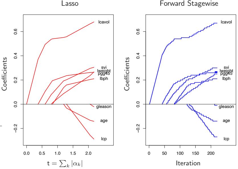
FIGURE 16.1. Profiles of estimated coefficients from linear regression, for the prostate data studied in Chapter 3. The left panel shows the results from the lasso, for different values of the bound parameter t = P ^k |αk|. The right panel shows the results of the stagewise linear regression Algorithm 16.1, using M = 220 consecutive steps of size ε = .01.

nal variables X^k themselves; that is, a multiple linear regression model. The left panel displays the profiles of estimated coefficients from the lasso, for different values of the bound parameter t = # ^k |αk|. The right panel shows the results of the stagewise Algorithm 16.1, with M = 250 and ε = 0.01. [The left and right panels of Figure 16.1 are the same as Figure 3.10 and the left panel of Figure 3.19, respectively.] The similarity between the two graphs is striking.

In some situations the resemblance is more than qualitative. For example, if all of the basis functions T^k are mutually uncorrelated, then as ε ↓ 0, M ↑ such that Mϵ → t, Algorithm 16.1 yields exactly the same solution as the lasso for bound parameter t = # ^k |αk| (and likewise for all solutions along the path). Of course, tree-based regressors are not uncorrelated. However, the solution sets are also identical if the coefficients ˆαk(λ) are all monotone functions of λ. This is often the case when the correlation between the variables is low. When the ˆαk(λ) are not monotone in λ, then the solution sets are not identical. The solution sets for Algorithm 16.1 tend to change less rapidly with changing values of the regularization parameter than those of the lasso.

610 16. Ensemble Learning

Efron et al. (2004) make the connections more precise, by characterizing the exact solution paths in the ε-limiting case. They show that the coefficient paths are piece-wise linear functions, both for the lasso and forward stagewise. This facilitates efficient algorithms which allow the entire paths to be computed with the same cost as a single least-squares fit. This least angle regression algorithm is described in more detail in Section 3.8.1.

Hastie et al. (2007) show that this infinitesimal forward stagewise algorithm (FS0) fits a monotone version of the lasso, which optimally reduces at each step the loss function for a given increase in the arc length of the coefficient path (see Sections 16.2.3 and 3.8.1). The arc-length for the ϵ > 0 case is Mϵ, and hence proportional to the number of steps.

Tree boosting (Algorithm 10.3) with shrinkage (10.41) closely resembles Algorithm 16.1, with the learning rate parameter ν corresponding to ε. For squared error loss, the only difference is that the optimal tree to be selected at each iteration Tk^∗ is approximated by the standard top-down greedy tree-induction algorithm. For other loss functions, such as the exponential loss of AdaBoost and the binomial deviance, Rosset et al. (2004a) show similar results to what we see here. Thus, one can view tree boosting with shrinkage as a form of monotone ill-posed regression on all possible (Jterminal node) trees, with the lasso penalty (16.4) as a regularizer. We return to this topic in Section 16.2.3.

The choice of no shrinkage [ν = 1 in equation (10.41)] is analogous to forward-stepwise regression, and its more aggressive cousin best-subset selection, which penalizes the number of non zero coefficients J(α) = # ^k |αk| 0. With a small fraction of dominant variables, best subset approaches often work well. But with a moderate fraction of strong variables, it is well known that subset selection can be excessively greedy (Copas, 1983), often yielding poor results when compared to less aggressive strategies such as the lasso or ridge regression. The dramatic improvements often seen when shrinkage is used with boosting are yet another confirmation of this approach.

16.2.2 The “Bet on Sparsity” Principle

As shown in the previous section, boosting’s forward stagewise strategy with shrinkage approximately minimizes the same loss function with a lasso-style L¹ penalty. The model is built up slowly, searching through “model space” and adding shrunken basis functions derived from important predictors. In contrast, the L² penalty is computationally much easier to deal with, as shown in Section 12.3.7. With the basis functions and L² penalty chosen to match a particular positive-definite kernel, one can solve the corresponding optimization problem without explicitly searching over individual basis functions.

However, the sometimes superior performance of boosting over procedures such as the support vector machine may be largely due to the implicit use of the L¹ versus L² penalty. The shrinkage resulting from the L¹ penalty is better suited to sparse situations, where there are few basis functions with nonzero coefficients (among all possible choices).

We can strengthen this argument through a simple example, taken from Friedman et al. (2004). Suppose we have 10, 000 data points and our model is a linear combination of a million trees. If the true population coefficients of these trees arose from a Gaussian distribution, then we know that in a Bayesian sense the best predictor is ridge regression (Exercise 3.6). That is, we should use an L² rather than an L¹ penalty when fitting the coefficients. On the other hand, if there are only a small number (e.g., 1000) coefficients that are nonzero, the lasso (L¹ penalty) will work better. We think of this as a sparse scenario, while the first case (Gaussian coefficients) is dense. Note however that in the dense scenario, although the L² penalty is best, neither method does very well since there is too little data from which to estimate such a large number of nonzero coefficients. This is the curse of dimensionality taking its toll. In a sparse setting, we can potentially do well with the L¹ penalty, since the number of nonzero coefficients is small. The L² penalty fails again.

In other words, use of the L¹ penalty follows what we call the “bet on sparsity” principle for high-dimensional problems:

Use a procedure that does well in sparse problems, since no procedure does well in dense problems.

These comments need some qualification:

• For any given application, the degree of sparseness/denseness depends on the unknown true target function, and the chosen dictionary T .
• The notion of sparse versus dense is relative to the size of the training data set and/or the noise-to-signal ratio (NSR). Larger training sets allow us to estimate coefficients with smaller standard errors. Likewise in situations with small NSR, we can identify more nonzero coefficients with a given sample size than in situations where the NSR is larger.
• The size of the dictionary plays a role as well. Increasing the size of the dictionary may lead to a sparser representation for our function, but the search problem becomes more difficult leading to higher variance.

Figure 16.2 illustrates these points in the context of linear models using simulation. We compare ridge regression and lasso, both for classification and regression problems. Each run has 50 observations with 300 independent Gaussian predictors. In the top row all 300 coefficients are nonzero, generated from a Gaussian distribution. In the middle row, only 10 are nonzero and generated from a Gaussian, and the last row has 30 non zero Gaussian coefficients. For regression, standard Gaussian noise is

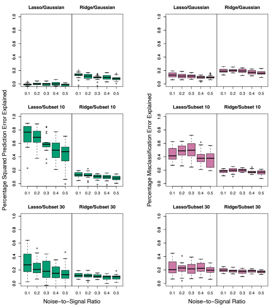
Regression

Classification

FIGURE 16.2. Simulations that show the superiority of the L¹ (lasso) penalty over L² (ridge) in regression and classification. Each run has 50 observations with 300 independent Gaussian predictors. In the top row all 300 coefficients are nonzero, generated from a Gaussian distribution. In the middle row, only 10 are nonzero, and the last row has 30 nonzero. Gaussian errors are added to the linear predictor η(X) for the regression problems, and binary responses generated via the inverse-logit transform for the classification problems. Scaling of η(X) resulted in the noise-to-signal ratios shown. Lasso is used in the left sub-columns, ridge in the right. We report the optimal percentage of error explained on test data (relative to the error of a constant model), displayed as boxplots over 20 realizations for each combination. In the only situation where ridge beats lasso (top row), neither do well.

added to the linear predictor η(X) = X^T β to produce a continuous response. For classification the linear predictor is transformed via the inverselogit to a probability, and a binary response is generated. Five different noise-to-signal ratios are presented, obtained by scaling η(X) prior to generating the response. In both cases this is defined to be NSR = Var(Y |η(X))/Var(η(X)). Both the ridge regression and lasso coefficient paths were fit using a series of 50 values of λ corresponding to a range of df from 1 to 50 (see Chapter 3 for details). The models were evaluated on a large test set (infinite for Gaussian, 5000 for binary), and in each case the value for λ was chosen to minimize the test-set error. We report percentage variance explained for the regression problems, and percentage misclassification error explained for the classification problems (relative to a baseline error of 0.5). There are 20 simulation runs for each scenario.

Note that for the classification problems, we are using squared-error loss to fit the binary response. Note also that we do not using the training data to select λ, but rather are reporting the best possible behavior for each method in the different scenarios. The L² penalty performs poorly everywhere. The Lasso performs reasonably well in the only two situations where it can (sparse coefficients). As expected the performance gets worse as the NSR increases (less so for classification), and as the model becomes denser. The differences are less marked for classification than for regression.

These empirical results are supported by a large body of theoretical results (Donoho and Johnstone, 1994; Donoho and Elad, 2003; Donoho, 2006b; Candes and Tao, 2007) that support the superiority of L¹ estimation in sparse settings.

16.2.3 Regularization Paths, Over-fitting and Margins

It has often been observed that boosting “does not overfit,” or more astutely is “slow to overfit.” Part of the explanation for this phenomenon was made earlier for random forests — misclassification error is less sensitive to variance than is mean-squared error, and classification is the major focus in the boosting community. In this section we show that the regularization paths of boosted models are “well behaved,” and that for certain loss functions they have an appealing limiting form.

Figure 16.3 shows the coefficient paths for lasso and infinitesimal forward stagewise (FS0) in a simulated regression setting. The data consists of a dictionary of 1000 Gaussian variables, strongly correlated (ρ = 0.95) within blocks of 20, but uncorrelated between blocks. The generating model has nonzero coefficients for 50 variables, one drawn from each block, and the coefficient values are drawn from a standard Gaussian. Finally, Gaussian noise is added, with a noise-to-signal ratio of 0.72 (Exercise 16.1.) The FS⁰ algorithm is a limiting form of algorithm 16.1, where the step size ε is shrunk to zero (Section 3.8.1). The grouping of the variables is intended to mimic the correlations of nearby trees, and with the forward-stagewise

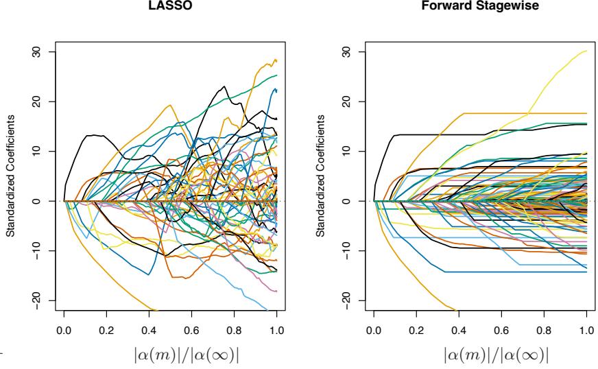
FIGURE 16.3. Comparison of lasso and infinitesimal forward stagewise paths on simulated regression data. The number of samples is 60 and the number of variables is 1000. The forward-stagewise paths fluctuate less than those of lasso in the final stages of the algorithms.

algorithm, this setup is intended as an idealized version of gradient boosting with shrinkage. For both these algorithms, the coefficient paths can be computed exactly, since they are piecewise linear (see the LARS algorithm in Section 3.8.1).

Here the coefficient profiles are similar only in the early stages of the paths. For the later stages, the forward stagewise paths tend to be monotone and smoother, while those for the lasso fluctuate widely. This is due to the strong correlations among subsets of the variables —lasso suffers somewhat from the multi-collinearity problem (Exercise 3.28).

The performance of the two models is rather similar (Figure 16.4), and they achieve about the same minimum. In the later stages forward stagewise takes longer to overfit, a likely consequence of the smoother paths.

Hastie et al. (2007) show that FS⁰ solves a monotone version of the lasso problem for squared error loss. Let ^{T a = T ∪} {−T } be the augmented dictionary obtained by including a negative copy of every basis element in ^T . We consider models ^f(x) = # ^Tk∈^{T a} αkTk(x) with non-negative coefficients α^k ≥ 0. In this expanded space, the lasso coefficient paths are positive, while those of FS⁰ are monotone nondecreasing.

The monotone lasso path is characterized by a differential equation

\[\frac{\partial \alpha}{\partial \ell} = \rho^{ml}(\alpha(\ell)),\tag{16.6}\]

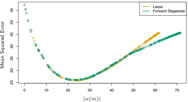
FIGURE 16.4. Mean squared error for lasso and infinitesimal forward stagewise on the simulated data. Despite the difference in the coefficient paths, the two models perform similarly over the critical part of the regularization path. In the right tail, lasso appears to overfit more rapidly.

with initial condition α(0) = 0, where ℓ is the L¹ arc-length of the path α(ℓ) (Exercise 16.2). The monotone lasso move direction (velocity vector) ρml(α(ℓ)) decreases the loss at the optimal quadratic rate per unit increase in the L¹ arc-length of the path. Since ρml ^k (α(ℓ)) ≥ 0 ∀k, ℓ, the solution paths are monotone.

The lasso can similarly be characterized as the solution to a differential equation as in (16.6), except that the move directions decrease the loss optimally per unit increase in the L¹ norm of the path. As a consequence, they are not necessarily positive, and hence the lasso paths need not be monotone.

In this augmented dictionary, restricting the coefficients to be positive is natural, since it avoids an obvious ambiguity. It also ties in more naturally with tree boosting—we always find trees positively correlated with the current residual.

There have been suggestions that boosting performs well (for two-class classification) because it exhibits maximal-margin properties, much like the support-vector machines of Chapters 4.5.2 and 12. Schapire et al. (1998) define the normalized L¹ margin of a fitted model f(x) = # ^k αkTk(x) as

\[m(f) = \min\_{i} \frac{y\_i f(x\_i)}{\sum\_{k=1}^{K} |\alpha\_k|}. \tag{16.7}\]

Here the minimum is taken over the training sample, and yⁱ ∈ {−1, +1}. Unlike the L² margin (4.40) of support vector machines, the L¹ margin m(f) measures the distance to the closest training point in L^∞ units (maximum coordinate distance).

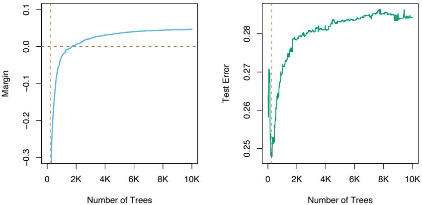
FIGURE 16.5. The left panel shows the L¹ margin m(f) for the Adaboost classifier on the mixture data, as a function of the number of 4-node trees. The model was fit using the R package gbm, with a shrinkage factor of 0.02. After 10, 000 trees, m(f) has settled down. Note that when the margin crosses zero, the training error becomes zero. The right panel shows the test error, which is minimized at 240 trees. In this case, Adaboost overfits dramatically if run to convergence.

Schapire et al. (1998) prove that with separable data, Adaboost increases m(f) with each iteration, converging to a margin-symmetric solution. R¨atsch and Warmuth (2002) prove the asymptotic convergence of Adaboost with shrinkage to a L1-margin-maximizing solution. Rosset et al. (2004a) consider regularized models of the form (16.2) for general loss functions. They show that as λ ↓ 0, for particular loss functions the solution converges to a margin-maximizing configuration. In particular they show this to be the case for the exponential loss of Adaboost, as well as binomial deviance.

Collecting together the results of this section, we reach the following summary for boosted classifiers:

The sequence of boosted classifiers form an L1-regularized monotone path to a margin-maximizing solution.

Of course the margin-maximizing end of the path can be a very poor, overfit solution, as it is in the example in Figure 16.5. Early stopping amounts to picking a point along the path, and should be done with the aid of a validation dataset.

16.3 Learning Ensembles

The insights learned from the previous sections can be harnessed to produce a more effective and efficient ensemble model. Again we consider functions of the form

\[f(x) = \alpha\_0 + \sum\_{T\_k \in T} \alpha\_k T\_k(x),\tag{16.8}\]

where T is a dictionary of basis functions, typically trees. For gradient boosting and random forests, |T | is very large, and it is quite typical for the final model to involve many thousands of trees. In the previous section we argue that gradient boosting with shrinkage fits an L¹ regularized monotone path in this space of trees.

Friedman and Popescu (2003) propose a hybrid approach which breaks this process down into two stages:

• A finite dictionary T^L = {T1(x), T2(x),…,TM(x)} of basis functions is induced from the training data;
• A family of functions fλ(x) is built by fitting a lasso path in this dictionary:

\[\alpha(\lambda) = \arg\min\_{\alpha} \sum\_{i=1}^{N} L[y\_i, \alpha\_0 + \sum\_{m=1}^{M} \alpha\_m T\_m(x\_i)] + \lambda \sum\_{m=1}^{M} |\alpha\_m|. \tag{16.9}\]

In its simplest form this model could be seen as a way of post-processing boosting or random forests, taking for T^L the collection of trees produced by the gradient boosting or random forest algorithms. By fitting the lasso path to these trees, we would typically use a much reduced set, which would save in computations and storage for future predictions. In the next section we describe modifications of this prescription that reduce the correlations in the ensemble TL, and improve the performance of the lasso post processor.

As an initial illustration, we apply this procedure to a random forest ensemble grown on the spam data.

Figure 16.6 shows that a lasso post-processing offers modest improvement over the random forest (blue curve), and reduces the forest to about 40 trees, rather than the original 1000. The post-processed performance matches that of gradient boosting. The orange curves represent a modified version of random forests, designed to reduce the correlations between trees even more. Here a random sub-sample (without replacement) of 5% of the training sample is used to grow each tree, and the trees are restricted to be shallow (about six terminal nodes). The post-processing offers more dramatic improvements here, and the training costs are reduced by a factor of about 100. However, the performance of the post-processed model falls somewhat short of the blue curves.

16.3.1 Learning a Good Ensemble

Not all ensembles T^L will perform well with post-processing. In terms of basis functions, we want a collection that covers the space well in places

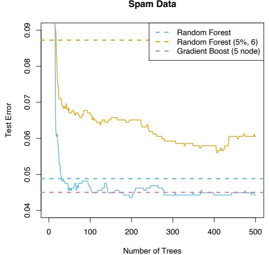
FIGURE 16.6. Application of the lasso post-processing (16.9) to the spam data. The horizontal blue line is the test error of a random forest fit to the spam data, using 1000 trees grown to maximum depth (with m = 7; see Algorithm 15.1). The jagged blue curve is the test error after post-processing the first 500 trees using the lasso, as a function of the number of trees with nonzero coefficients. The orange curve/line use a modified form of random forest, where a random draw of 5% of the data are used to grow each tree, and the trees are forced to be shallow (typically six terminal nodes). Here the post-processing offers much greater improvement over the random forest that generated the ensemble.

where they are needed, and are sufficiently different from each other for the post-processor to be effective.

Friedman and Popescu (2003) gain insights from numerical quadrature and importance sampling. They view the unknown function as an integral

\[f(x) = \int \beta(\gamma)b(x;\gamma)d\gamma,\tag{16.10}\]

where γ ∈ Γ indexes the basis functions b(x; γ). For example, if the basis functions are trees, then γ indexes the splitting variables, the split-points and the values in the terminal nodes. Numerical quadrature amounts to finding a set of M evaluation points γ^m ∈ Γ and corresponding weights α^m so that fM(x) = α⁰ + #^{M m}=1 αmb(x; γm) approximates f(x) well over the domain of x. Importance sampling amounts to sampling γ at random, but giving more weight to relevant regions of the space Γ. Friedman and Popescu (2003) suggest a measure of (lack of) relevance that uses the loss function (16.9):

16.3 Learning Ensembles 619

\[Q(\gamma) = \min\_{c\_0, c\_1} \sum\_{i=1}^{N} L(y\_i, c\_0 + c\_1 b(x\_i; \gamma)),\tag{16.11}\]

evaluated on the training data.

If a single basis function were to be selected (e.g., a tree), it would be the global minimizer γ^∗ = arg minγ∈^Γ Q(γ). Introducing randomness in the selection of γ would necessarily produce less optimal values with Q(γ) ≥ Q(γ^∗). They propose a natural measure of the characteristic width σ of the sampling scheme S,

\[ \sigma = \mathcal{E}\_{\mathcal{S}}[Q(\gamma) - Q(\gamma^\*)].\tag{16.12} \]

• σ too narrow suggests too many of the b(x; γm) look alike, and similar to b(x; γ^∗);
• σ too wide implies a large spread in the b(x; γm), but possibly consisting of many irrelevant cases.

Friedman and Popescu (2003) use sub-sampling as a mechanism for introducing randomness, leading to their ensemble-generation algorithm 16.2.

Algorithm 16.2 ISLE Ensemble Generation.

• 1. f0(x) = arg min^c #^{N i}=1 L(yi, c)
• 2. For m = 1 to M do
  • 1. γ^m = arg min^γ # ⁱ∈Sm(η) L(yi, fm−1(xi) + b(xi; γ))
  • 2. fm(x) = fm−1(x) + νb(x; γm)
• 3. TISLE = {b(x; γ1), b(x; γ2),…,b(x; γ^M )}.

Sm(η) refers to a subsample of N · η (η ∈ (0, 1]) of the training observations, typically without replacement. Their simulations suggest picking ^{η ≤ 1 2} , and for large N picking η ∼ 1/ √ N. Reducing η increases the randomness, and hence the width σ. The parameter ν ∈ [0, 1] introduces memory into the randomization process; the larger ν, the more the procedure avoids b(x; γ) similar to those found before. A number of familiar randomization schemes are special cases of Algorithm 16.2:

Bagging has η = 1, but samples with replacement, and has ν = 0. Friedman and Hall (2007) argue that sampling without replacement with η = 1/2 is equivalent to sampling with replacement with η = 1, and the former is much more efficient.

620 16. Ensemble Learning

• Random forest sampling is similar, with more randomness introduced by the selection of the splitting variable. Reducing η < 1/2 in algorithm 16.2 has a similar effect to reducing m in random forests, but does not suffer from the potential biases discussed in Section 15.4.2.
• Gradient boosting with shrinkage (10.41) uses η = 1, but typically does not produce sufficient width σ.

Stochastic gradient boosting (Friedman, 1999) follows the recipe exactly.

The authors recommend values ^ν = 0.1 and ^{η ≤ 1 2} , and call their combined procedure (ensemble generation and post processing) Importance sampled learning ensemble (ISLE).

Figure 16.7 shows the performance of an ISLE on the spam data. It does

FIGURE 16.7. Importance sampling learning ensemble (ISLE) fit to the spam data. Here we used η = 1/2, ν = 0.05, and trees with five terminal nodes. The lasso post-processed ensemble does not improve the prediction error in this case, but it reduces the number of trees by a factor of five.

not improve the predictive performance, but is able to produce a more parsimonious model. Note that in practice the post-processing includes the selection of the regularization parameter λ in (16.9), which would be chosen by cross-validation. Here we simply demonstrate the effects of postprocessing by showing the entire path on the test data.

Figure 16.8 shows various ISLEs on a regression example. The generating

FIGURE 16.8. Demonstration of ensemble methods on a regression simulation example. The notation GBM (0.1, 0.01) refers to a gradient boosted model, with parameters (η, ν). We report mean-squared error from the true (known) function. Note that the sub-sampled GBM model (green) outperforms the full GBM model (orange). The lasso post-processed version achieves similar error. The random forest is outperformed by its post-processed version, but both fall short of the other models.

function is

\[f(X) = 10 \cdot \prod\_{j=1}^{5} e^{-2X\_j^2} + \sum\_{j=6}^{35} X\_j,\tag{16.13}\]

where ^{X ∼ U}[0, 1]¹⁰⁰ (the last 65 elements are noise variables). The response ^{Y = f}(X) + ^ε where ^{ε ∼ N}(0, ^σ2); we chose ^σ = 1.3 resulting in a signal-to-noise ratio of approximately 2. We used a training sample of size 1000, and estimated the mean squared error E( ^ˆf(X)−f(X))² by averaging over a test set of 500 samples. The sub-sampled GBM curve (light blue) is an instance of stochastic gradient boosting (Friedman, 1999) discussed in Section 10.12, and it outperforms gradient boosting on this example.

622 16. Ensemble Learning

16.3.2 Rule Ensembles

Here we describe a modification of the tree-ensemble method that focuses on individual rules (Friedman and Popescu, 2003). We encountered rules in Section 9.3 in the discussion of the PRIM method. The idea is to enlarge an ensemble of trees by constructing a set of rules from each of the trees in the collection.

FIGURE 16.9. A typical tree in an ensemble, from which rules can be derived.

Figure 16.9 depicts a small tree, with numbered nodes. The following rules can be derived from this tree:

\[\begin{array}{lcl}R\_1(X) &=& I(X\_1 < 2.1) \\ R\_2(X) &=& I(X\_1 \ge 2.1) \\ R\_3(X) &=& I(X\_1 \ge 2.1) \cdot I(X\_3 \in \{S\}) \\ R\_4(X) &=& I(X\_1 \ge 2.1) \cdot I(X\_3 \in \{M, L\}) \\ R\_5(X) &=& I(X\_1 \ge 2.1) \cdot I(X\_3 \in \{S\}) \cdot I(X\_7 < 4.5) \\ R\_6(X) &=& I(X\_1 \ge 2.1) \cdot I(X\_3 \in \{S\}) \cdot I(X\_7 \ge 4.5) \end{array} \tag{16.14}\]

A linear expansion in rules 1, 4, 5 and 6 is equivalent to the tree itself (Exercise 16.3); hence (16.14) is an over-complete basis for the tree.

For each tree T^m in an ensemble T , we can construct its mini-ensemble of rules ^{T m} RULE, and then combine them all to form a larger ensemble

\[\mathcal{T}\_{\text{RULE}} = \bigcup\_{m=1}^{M} \mathcal{T}\_{\text{RULE}}^{m}. \tag{16.15}\]

This is then treated like any other ensemble, and post-processed via the lasso or similar regularized procedure.

There are several advantages to this approach of deriving rules from the more complex trees:

• The space of models is enlarged, and can lead to improved performance.

FIGURE 16.10. Mean squared error for rule ensembles, using 20 realizations of the simulation example (16.13).

• Rules are easier to interpret than trees, so there is the potential for a simplified model.
• It is often natural to augment T RULE by including each variable X^j separately as well, thus allowing the ensemble to model linear functions well.

Friedman and Popescu (2008) demonstrate the power of this procedure on a number of illustrative examples, including the simulation example (16.13). Figure 16.10 shows boxplots of the mean-squared error from the true model for twenty realizations from this model. The models were all fit using the Rulefit software, available on the ESL homepage³, which runs in an automatic mode.

On the same training set as used in Figure 16.8, the rule based model achieved a mean-squared error of 1.06. Although slightly worse than the best achieved in that figure, the results are not comparable because crossvalidation was used here to select the final model.

Bibliographic Notes

As noted in the introduction, many of the new methods in machine learning have been dubbed “ensemble” methods. These include neural networks boosting, bagging and random forests; Dietterich (2000a) gives a survey of tree-based ensemble methods. Neural networks (Chapter 11) are perhaps more deserving of the name, since they simultaneously learn the parameters

³ESL homepage: www-stat.stanford.edu/ElemStatLearn

624 16. Ensemble Learning

of the hidden units (basis functions), along with how to combine them. Bishop (2006) discusses neural networks in some detail, along with the Bayesian perspective (MacKay, 1992; Neal, 1996). Support vector machines (Chapter 12) can also be regarded as an ensemble method; they perform L² regularized model fitting in high-dimensional feature spaces. Boosting and lasso exploit sparsity through L¹ regularization to overcome the highdimensionality, while SVMs rely on the “kernel trick” characteristic of L² regularization.

C5.0 (Quinlan, 2004) is a commercial tree and rule generation package, with some goals in common with Rulefit.

There is a vast and varied literature often referred to as “combining classifiers” which abounds in ad-hoc schemes for mixing methods of different types to achieve better performance. For a principled approach, see Kittler et al. (1998).

Exercises

Ex. 16.1 Describe exactly how to generate the block correlated data used in the simulation in Section 16.2.3.

Ex. 16.2 Let ^α(t) ^∈ IR^p be a piecewise-differentiable and continuous coefficient profile, with α(0) = 0. The L¹ arc-length of α from time 0 to t is defined by

\[ \Lambda(t) = \int\_0^t |\dot{\alpha}(t)|\_1 dt. \tag{16.16} \]

Show that Λ(t) ≥ |α(t)|1, with equality iff α(t) is monotone.

Ex. 16.3 Show that fitting a linear regression model using rules 1, 4, 5 and 6 in equation (16.14) gives the same fit as the regression tree corresponding to this tree. Show the same is true for classification, if a logistic regression model is fit.

Ex. 16.4 Program and run the simulation study described in Figure 16.2.

This is page 625 Printer: Opaque this

17 Undirected Graphical Models

17.1 Introduction

A graph consists of a set of vertices (nodes), along with a set of edges joining some pairs of the vertices. In graphical models, each vertex represents a random variable, and the graph gives a visual way of understanding the joint distribution of the entire set of random variables. They can be useful for either unsupervised or supervised learning. In an undirected graph, the edges have no directional arrows. We restrict our discussion to undirected graphical models, also known as Markov random fields or Markov networks. In these graphs, the absence of an edge between two vertices has a special meaning: the corresponding random variables are conditionally independent, given the other variables.

Figure 17.1 shows an example of a graphical model for a flow-cytometry dataset with p = 11 proteins measured on N = 7466 cells, from Sachs et al. (2003). Each vertex in the graph corresponds to the real-valued expression level of a protein. The network structure was estimated assuming a multivariate Gaussian distribution, using the graphical lasso procedure discussed later in this chapter.

Sparse graphs have a relatively small number of edges, and are convenient for interpretation. They are useful in a variety of domains, including genomics and proteomics, where they provide rough models of cell pathways. Much work has been done in defining and understanding the structure of graphical models; see the Bibliographic Notes for references.

626 17. Undirected Graphical Models

FIGURE 17.1. Example of a sparse undirected graph, estimated from a flow cytometry dataset, with p = 11 proteins measured on N = 7466 cells. The network structure was estimated using the graphical lasso procedure discussed in this chapter.

As we will see, the edges in a graph are parametrized by values or potentials that encode the strength of the conditional dependence between the random variables at the corresponding vertices. The main challenges in working with graphical models are model selection (choosing the structure of the graph), estimation of the edge parameters from data, and computation of marginal vertex probabilities and expectations, from their joint distribution. The last two tasks are sometimes called learning and inference in the computer science literature.

We do not attempt a comprehensive treatment of this interesting area. Instead, we introduce some basic concepts, and then discuss a few simple methods for estimation of the parameters and structure of undirected graphical models; methods that relate to the techniques already discussed in this book. The estimation approaches that we present for continuous and discrete-valued vertices are different, so we treat them separately. Sections 17.3.1 and 17.3.2 may be of particular interest, as they describe new, regression-based procedures for estimating graphical models.

There is a large and active literature on directed graphical models or Bayesian networks; these are graphical models in which the edges have directional arrows (but no directed cycles). Directed graphical models represent probability distributions that can be factored into products of conditional distributions, and have the potential for causal interpretations. We refer the reader to Wasserman (2004) for a brief overview of both undirected and directed graphs; the next section follows closely his Chapter 18.

FIGURE 17.2. Examples of undirected graphical models or Markov networks. Each node or vertex represents a random variable, and the lack of an edge between two nodes indicates conditional independence. For example, in graph (a), X and Z are conditionally independent, given Y . In graph (b), Z is independent of each of X, Y , and W.

A longer list of useful references is given in the Bibliographic Notes on page 645.

17.2 Markov Graphs and Their Properties

In this section we discuss the basic properties of graphs as models for the joint distribution of a set of random variables. We defer discussion of (a) parametrization and estimation of the edge parameters from data, and (b) estimation of the topology of a graph, to later sections.

Figure 17.2 shows four examples of undirected graphs. A graph G consists of a pair (V,E), where V is a set of vertices and E the set of edges (defined by pairs of vertices). Two vertices X and Y are called adjacent if there is a edge joining them; this is denoted by X ∼ Y . A path X1, X2,…,Xⁿ is a set of vertices that are joined, that is Xi−¹ ∼ Xⁱ for i = 2,…,n. A complete graph is a graph with every pair of vertices joined by an edge. A subgraph U ∈ V is a subset of vertices together with their edges. For example, (X, Y, Z) in Figure 17.2(a) form a path but not a complete graph.

Suppose that we have a graph G whose vertex set V represents a set of random variables having joint distribution P. In a Markov graph G, the absence of an edge implies that the corresponding random variables are conditionally independent given the variables at the other vertices. This is expressed with the following notation:

628 17. Undirected Graphical Models

No edge joining X and Y ⇐⇒ X ⊥ Y |rest (17.1)

where “rest” refers to all of the other vertices in the graph. For example in Figure 17.2(a) X ⊥ Z|Y . These are known as the pairwise Markov independencies of G.

If A, B and C are subgraphs, then C is said to separate A and B if every path between A and B intersects a node in C. For example, Y separates X and Z in Figures 17.2(a) and (d), and Z separates Y and W in (d). In Figure 17.2(b) Z is not connected to X, Y,W so we say that the two sets are separated by the empty set. In Figure 17.2(c), C = {X, Z} separates Y and W.

Separators have the nice property that they break the graph into conditionally independent pieces. Specifically, in a Markov graph G with subgraphs A, B and C,

\[\text{If } C \text{ separates } A \text{ and } B \text{ then } A \perp B | C. \tag{17.2}\]

These are known as the global Markov properties of G. It turns out that the pairwise and global Markov properties of a graph are equivalent (for graphs with positive distributions). That is, the set of graphs with associated probability distributions that satisfy the pairwise Markov independencies and global Markov assumptions are the same. This result is useful for inferring global independence relations from simple pairwise properties. For example in Figure 17.2(d) X ⊥ Z|{Y,W} since it is a Markov graph and there is no link joining X and Z. But Y also separates X from Z and W and hence by the global Markov assumption we conclude that X ⊥ Z|Y and X ⊥ W|Y . Similarly we have Y ⊥ W|Z.

The global Markov property allows us to decompose graphs into smaller more manageable pieces and thus leads to essential simplifications in computation and interpretation. For this purpose we separate the graph into cliques. A clique is a complete subgraph— a set of vertices that are all adjacent to one another; it is called maximal if it is a clique and no other vertices can be added to it and still yield a clique. The maximal cliques for the graphs of Figure 17.2 are

• 1. {X, Y }, {Y,Z},
• 2. {X, Y,W}, {Z},
• 3. {X, Y }, {Y,Z}, {Z,W}, {X,W}, and
• 4. {X, Y }, {Y,Z}, {Z,W}.

Although the following applies to both continuous and discrete distributions, much of the development has been for the latter. A probability density function f over a Markov graph G can be can represented as

17.2 Markov Graphs and Their Properties 629

\[f(x) = \frac{1}{Z} \prod\_{C \in \mathcal{C}} \psi\_C(x\_C) \tag{17.3}\]

where C is the set of maximal cliques, and the positive functions ψ^C (·) are called clique potentials. These are not in general density functions1, but rather are affinities that capture the dependence in X^C by scoring certain instances x^C higher than others. The quantity

\[Z = \sum\_{x \in \mathcal{X}} \prod\_{C \in \mathcal{C}} \psi\_C(x\_C) \tag{17.4}\]

is the normalizing constant, also known as the partition function. Alternatively, the representation (17.3) implies a graph with independence properties defined by the cliques in the product. This result holds for Markov networks G with positive distributions, and is known as the Hammersley-Clifford theorem (Hammersley and Clifford, 1971; Clifford, 1990).

Many of the methods for estimation and computation on graphs first decompose the graph into its maximal cliques. Relevant quantities are computed in the individual cliques and then accumulated across the entire graph. A prominent example is the join tree or junction tree algorithm for computing marginal and low order probabilities from the joint distribution on a graph. Details can be found in Pearl (1986), Lauritzen and Spiegelhalter (1988), Pearl (1988), Shenoy and Shafer (1988), Jensen et al. (1990), or Koller and Friedman (2007).

FIGURE 17.3. A complete graph does not uniquely specify the higher-order dependence structure in the joint distribution of the variables.

A graphical model does not always uniquely specify the higher-order dependence structure of a joint probability distribution. Consider the complete three-node graph in Figure 17.3. It could represent the dependence structure of either of the following distributions:

\[\begin{array}{rcl}f^{(2)}(x,y,z)&=&\frac{1}{Z}\psi(x,y)\psi(x,z)\psi(y,z);\\f^{(3)}(x,y,z)&=&\frac{1}{Z}\psi(x,y,z).\end{array} \tag{17.5}\]

The first specifies only second order dependence (and can be represented with fewer parameters). Graphical models for discrete data are a special

¹If the cliques are separated, then the potentials can be densities, but this is in general not the case.

630 17. Undirected Graphical Models

case of loglinear models for multiway contingency tables (Bishop et al., 1975, e.g.); in that language f(2) is referred to as the “no second-order interaction” model.

For the remainder of this chapter we focus on pairwise Markov graphs (Koller and Friedman, 2007). Here there is a potential function for each edge (pair of variables as in f(2) above), and at most second–order interactions are represented. These are more parsimonious in terms of parameters, easier to work with, and give the minimal complexity implied by the graph structure. The models for both continuous and discrete data are functions of only the pairwise marginal distributions of the variables represented in the edge set.

17.3 Undirected Graphical Models for Continuous Variables

Here we consider Markov networks where all the variables are continuous. The Gaussian distribution is almost always used for such graphical models, because of its convenient analytical properties. We assume that the observations have a multivariate Gaussian distribution with mean µ and covariance matrix Σ. Since the Gaussian distribution represents at most second-order relationships, it automatically encodes a pairwise Markov graph. The graph in Figure 17.1 is an example of a Gaussian graphical model.

The Gaussian distribution has the property that all conditional distributions are also Gaussian. The inverse covariance matrix Σ⁻¹ contains information about the partial covariances between the variables; that is, the covariances between pairs i and j, conditioned on all other variables. In particular, if the ijth component of Θ = Σ⁻¹ is zero, then variables i and j are conditionally independent, given the other variables (Exercise 17.3).

It is instructive to examine the conditional distribution of one variable versus the rest, where the role of Θ is explicit. Suppose we partition X = (Z, Y ) where Z = (X1,…,Xp−1) consists of the first p − 1 variables and Y = X^p is the last. Then we have the conditional distribution of Y give Z (Mardia et al., 1979, e.g.)

\[Y|Z=z \sim N\left(\mu\_Y + (z-\mu\_Z)^T \Sigma\_{ZZ}^{-1} \sigma\_{ZY}, \ \sigma\_{YY} - \sigma\_{ZY}^T \Sigma\_{ZZ}^{-1} \sigma\_{ZY}\right), \tag{17.6}\]

where we have partitioned Σ as

\[ \Sigma = \begin{pmatrix} \Sigma\_{ZZ} & \sigma\_{ZY} \\ \sigma\_{ZY}^T & \sigma\_{YY} \end{pmatrix}. \tag{17.7} \]

The conditional mean in (17.6) has exactly the same form as the population multiple linear regression of Y on Z, with regression coefficient β = Σ−¹ ZZσZY [see (2.16) on page 19]. If we partition Θ in the same way, since ΣΘ = I standard formulas for partitioned inverses give

17.3 Undirected Graphical Models for Continuous Variables 631

\[ \theta\_{ZY} = -\theta\_{YY} \cdot \Sigma\_{ZZ}^{-1} \sigma\_{ZY}, \tag{17.8} \]

where 1/θY Y ^{= σ}Y Y ^{− σT} ZY Σ⁻¹ ZZσZY > 0. Hence

\[ \begin{array}{rcl} \beta &=& \Sigma\_{ZZ}^{-1} \sigma\_{ZY} \\ &=& -\theta\_{ZY}/\theta\_{YY} . \end{array} \tag{17.9} \]

We have learned two things here:

• The dependence of Y on Z in (17.6) is in the mean term alone. Here we see explicitly that zero elements in β and hence θZY mean that the corresponding elements of Z are conditionally independent of Y , given the rest.
• We can learn about this dependence structure through multiple linear regression.

Thus Θ captures all the second-order information (both structural and quantitative) needed to describe the conditional distribution of each node given the rest, and is the so-called “natural” parameter for the Gaussian graphical model².

Another (different) kind of graphical model is the covariance graph or relevance network, in which vertices are connected by bidirectional edges if the covariance (rather than the partial covariance) between the corresponding variables is nonzero. These are popular in genomics, see especially Butte et al. (2000). The negative log-likelihood from these models is not convex, making the computations more challenging (Chaudhuri et al., 2007).

17.3.1 Estimation of the Parameters when the Graph Structure is Known

Given some realizations of X, we would like to estimate the parameters of an undirected graph that approximates their joint distribution. Suppose first that the graph is complete (fully connected). We assume that we have N multivariate normal realizations xi, i = 1,…,N with population mean µ and covariance Σ. Let

\[\mathbf{S} = \frac{1}{N} \sum\_{i=1}^{N} (x\_i - \bar{x})(x\_i - \bar{x})^T \tag{17.10}\]

be the empirical covariance matrix, with ¯x the sample mean vector. Ignoring constants, the log-likelihood of the data can be written as

²The distribution arising from a Gaussian graphical model is a Wishart distribution. This is a member of the exponential family, with canonical or “natural” parameter Θ = Σ−1. Indeed, the partially maximized log-likelihood (17.11) is (up to constants) the Wishart log-likelihood.

632 17. Undirected Graphical Models

\[\ell(\boldsymbol{\Theta}) = \log \det \boldsymbol{\Theta} - \text{trace}(\mathbf{S}\boldsymbol{\Theta}).\tag{17.11}\]

In (17.11) we have partially maximized with respect to the mean parameter µ. The quantity −ℓ(Θ) is a convex function of Θ. It is easy to show that the maximum likelihood estimate of Σ is simply S.

Now to make the graph more useful (especially in high-dimensional settings) let’s assume that some of the edges are missing; for example, the edge between PIP3 and Erk is one of several missing in Figure 17.1. As we have seen, for the Gaussian distribution this implies that the corresponding entries of Θ = Σ⁻¹ are zero. Hence we now would like to maximize (17.11) under the constraints that some pre-defined subset of the parameters are zero. This is an equality-constrained convex optimization problem, and a number of methods have been proposed for solving it, in particular the iterative proportional fitting procedure (Speed and Kiiveri, 1986). This and other methods are summarized for example in Whittaker (1990) and Lauritzen (1996). These methods exploit the simplifications that arise from decomposing the graph into its maximal cliques, as described in the previous section. Here we outline a simple alternate approach, that exploits the sparsity in a different way. The fruits of this approach will become apparent later when we discuss the problem of estimation of the graph structure.

The idea is based on linear regression, as inspired by (17.6) and (17.9). In particular, suppose that we want to estimate the edge parameters θij for the vertices that are joined to a given vertex i, restricting those that are not joined to be zero. Then it would seem that the linear regression of the node i values on the other relevant vertices might provide a reasonable estimate. But this ignores the dependence structure among the predictors in this regression. It turns out that if instead we use our current (model-based) estimate of the cross-product matrix of the predictors when we perform our regressions, this gives the correct solutions and solves the constrained maximum-likelihood problem exactly. We now give details.

To constrain the log-likelihood (17.11), we add Lagrange constants for all missing edges

\[\ell\_C(\Theta) = \log \det \Theta - \text{trace}(\mathbf{S}\Theta) - \sum\_{(j,k)\notin E} \gamma\_{jk}\theta\_{jk}.\tag{17.12}\]

The gradient equation for maximizing (17.12) can be written as

\[ \Theta^{-1} - \mathbf{S} - \Gamma = \mathbf{0}, \tag{17.13} \]

using the fact that the derivative of log det Θ equals Θ−¹ (Boyd and Vandenberghe, 2004, for example, page 641). Γ is a matrix of Lagrange parameters with nonzero values for all pairs with edges absent.

We will show how we can use regression to solve for Θ and its inverse W = Θ−¹ one row and column at a time. For simplicity let’s focus on the last row and column. Then the upper right block of equation (17.13) can be written as

17.3 Undirected Graphical Models for Continuous Variables 633

\[w\_{12} - s\_{12} - \gamma\_{12} = 0.\tag{17.14}\]

Here we have partitioned the matrices into two parts as in (17.7): part 1 being the first p−1 rows and columns, and part 2 the pth row and column. With W and its inverse Θ partitioned in a similar fashion, we have

\[ \begin{pmatrix} \mathbf{W}\_{11} & w\_{12} \\ w\_{12}^T & w\_{22} \end{pmatrix} \begin{pmatrix} \boldsymbol{\Theta}\_{11} & \boldsymbol{\theta}\_{12} \\ \boldsymbol{\theta}\_{12}^T & \boldsymbol{\theta}\_{22} \end{pmatrix} = \begin{pmatrix} \mathbf{I} & \mathbf{0} \\ \boldsymbol{0}^T & 1 \end{pmatrix}. \tag{17.15} \]

This implies

\[w\_{12} \quad = \ -\mathbf{W}\_{11}\theta\_{12}/\theta\_{22} \tag{17.16}\]

\[=\begin{array}{c}\mathbf{W}\_{11}\boldsymbol{\beta}\tag{17.17}\]

where β = −θ12/θ²² as in (17.9). Now substituting (17.17) into (17.14) gives

\[\mathbf{W}\_{11}\boldsymbol{\beta} - s\_{12} - \gamma\_{12} = 0.\tag{17.18}\]

These can be interpreted as the p − 1 estimating equations for the constrained regression of X^p on the other predictors, except that the observed mean cross-products matrix S¹¹ is replaced by W11, the current estimated covariance matrix from the model.

Now we can solve (17.18) by simple subset regression. Suppose there are p−q nonzero elements in γ12—i.e., p−q edges constrained to be zero. These p − q rows carry no information and can be removed. Furthermore we can reduce ^β to ^β∗ by removing its ^{p − q} zero elements, yielding the reduced q × q system of equations

\[\mathbf{W}\_{11}^\* \beta^\* - s\_{12}^\* = 0,\tag{17.19}\]

with solution βˆ^∗ = W^∗ 11−¹s^{∗ 12}. This is padded with ^{p − q} zeros to give ^βˆ.

Although it appears from (17.16) that we only recover the elements θ¹² up to a scale factor 1/θ22, it is easy to show that

\[\frac{1}{\theta\_{22}} = w\_{22} - w\_{12}^T \beta \tag{17.20}\]

(using partitioned inverse formulas). Also w²² = s22, since the diagonal of Γ in (17.13) is zero.

This leads to the simple iterative procedure given in Algorithm 17.1 for estimating both Wˆ and its inverse Θˆ , subject to the constraints of the missing edges.

Note that this algorithm makes conceptual sense. The graph estimation problem is not p separate regression problems, but rather p coupled problems. The use of the common W in step (b), in place of the observed cross-products matrix, couples the problems together in the appropriate fashion. Surprisingly, we were not able to find this procedure in the literature. However it is related to the covariance selection procedures of Algorithm 17.1 A Modified Regression Algorithm for Estimation of an Undirected Gaussian Graphical Model with Known Structure.

1. Initialize W = S.

• 2. Repeat for j = 1, 2, . . . , p, 1, 2, . . . , p, . . . until convergence:
  • 1. Partition the matrix W into part 1: all but the jth row and column, and part 2: the jth row and column.
  • 2. Solve W^{∗ 11}β^{∗ − s∗ 12} = 0 for the unconstrained edge parameters β^∗, using the reduced system of equations as in (17.19). Obtain βˆ by padding βˆ^∗ with zeros in the appropriate positions.
  • 3. Update w¹² = W11βˆ
• 3. In the final cycle (for each ^j) solve for ^ˆθ^{12 = −}β^ˆ · ^ˆθ22, with 1/ˆθ^{22 = s22 − wT 12}βˆ.

FIGURE 17.4. A simple graph for illustration, along with the empirical covariance matrix.

Dempster (1972), and is similar in flavor to the iterative conditional fitting procedure for covariance graphs, proposed by Chaudhuri et al. (2007).

Here is a little example, borrowed from Whittaker (1990). Suppose that our model is as depicted in Figure 17.4, along with its empirical covariance matrix S. We apply algorithm (17.1) to this problem; for example, in the modified regression for variable 1 in step (b), variable 3 is left out. The procedure quickly converged to the solutions:

\[ \hat{\Sigma} = \begin{pmatrix} 10.00 & 1.00 & 1.31 & 4.00 \\ 1.00 & 10.00 & 2.00 & 0.87 \\ 1.31 & 2.00 & 10.00 & 3.00 \\ 4.00 & 0.87 & 3.00 & 10.00 \end{pmatrix}, \quad \hat{\Sigma}^{-1} = \begin{pmatrix} 0.12 & -0.01 & 0.00 & -0.05 \\ -0.01 & 0.11 & -0.02 & 0.00 \\ 0.00 & -0.02 & 0.11 & -0.03 \\ -0.05 & 0.00 & -0.03 & 0.13 \end{pmatrix}. \]

Note the zeroes in Σˆ ⁻1, corresponding to the missing edges (1,3) and (2,4). Note also that the corresponding elements in Σˆ are the only elements different from S. The estimation of Σˆ is an example of what is sometimes called the positive definite “completion” of S.

17.3.2 Estimation of the Graph Structure

In most cases we do not know which edges to omit from our graph, and so would like to try to discover this from the data itself. In recent years a number of authors have proposed the use of L¹ (lasso) regularization for this purpose.

Meinshausen and B¨uhlmann (2006) take a simple approach to the problem: rather than trying to fully estimate Σ or Θ = Σ⁻1, they only estimate which components of θij are nonzero. To do this, they fit a lasso regression using each variable as the response and the others as predictors. The component θij is then estimated to be nonzero if either the estimated coefficient of variable i on j is nonzero, or the estimated coefficient of variable j on i is nonzero (alternatively they use an and rule). They show that asymptotically this procedure consistently estimates the set of nonzero elements of Θ.

We can take a more systematic approach with the lasso penalty, following the development of the previous section. Consider maximizing the penalized log-likelihood

\[\log \det \Theta - \text{trace} (\mathbf{S} \Theta) - \lambda ||\Theta||\_1,\tag{17.21}\]

where ||Θ||¹ is the L¹ norm—the sum of the absolute values of the elements of Σ⁻¹, and we have ignored constants. The negative of this penalized likelihood is a convex function of Θ.

It turns out that one can adapt the lasso to give the exact maximizer of the penalized log-likelihood. In particular, we simply replace the modified regression step (b) in Algorithm 17.1 by a modified lasso step. Here are the details.

The analog of the gradient equation (17.13) is now

\[\Theta^{-1} - \mathbf{S} - \lambda \cdot \text{Sign}(\Theta) = \mathbf{0}.\tag{17.22}\]

Here we use sub-gradient notation, with Sign(θjk) = sign(θjk) if θjk ̸= 0, else Sign(θjk) ∈ [−1, 1] if θjk = 0. Continuing the development in the previous section, we reach the analog of (17.18)

\[\mathbf{W}\_{11}\boldsymbol{\beta} - s\_{12} + \lambda \cdot \text{Sign}(\boldsymbol{\beta}) = 0 \tag{17.23}\]

(recall that β and θ¹² have opposite signs). We will now see that this system is exactly equivalent to the estimating equations for a lasso regression.

Consider the usual regression setup with outcome variables y and predictor matrix Z. There the lasso minimizes

\[\frac{1}{2}(\mathbf{y} - \mathbf{Z}\beta)^T(\mathbf{y} - \mathbf{Z}\beta) + \lambda \cdot ||\beta||\_1 \tag{17.24}\]

[see (3.52) on page 68; here we have added a factor ^{1 2} for convenience]. The gradient of this expression is

Algorithm 17.2 Graphical Lasso.

• 1. Initialize W = S + λI. The diagonal of W remains unchanged in what follows.
• 2. Repeat for j = 1, 2, . . . p, 1, 2, . . . p, . . . until convergence:
  • 1. Partition the matrix W into part 1: all but the jth row and column, and part 2: the jth row and column.
  • 2. Solve the estimating equations W11β − s¹² + λ · Sign(β)=0 using the cyclical coordinate-descent algorithm (17.26) for the modified lasso.
  • 3. Update w¹² = W11βˆ
• 3. In the final cycle (for each ^j) solve for ^ˆθ^{12 = −}β^ˆ · ^ˆθ22, with 1/ˆθ^{22 = w22 − wT 12}βˆ.

\[\mathbf{Z}^T \mathbf{Z} \beta - \mathbf{Z}^T \mathbf{y} + \lambda \cdot \text{Sign}(\beta) = 0 \tag{17.25}\]

So up to a factor 1/N, Z^T y is the analog of s12, and we replace Z^T Z by W11, the estimated cross-product matrix from our current model.

The resulting procedure is called the graphical lasso, proposed by Friedman et al. (2008b) building on the work of Banerjee et al. (2008). It is summarized in Algorithm 17.2.

Friedman et al. (2008b) use the pathwise coordinate descent method (Section 3.8.6) to solve the modified lasso problem at each stage. Here are the details of pathwise coordinate descent for the graphical lasso algorithm. Letting V = W11, the update has the form

\[ \beta\_j \gets S\left(s\_{12j} - \sum\_{k \neq j} V\_{kj}\beta\_k, \lambda\right) / V\_{jj} \tag{17.26} \]

for j = 1, 2,…,p − 1, 1, 2,…,p − 1,…, where S is the soft-threshold operator:

\[S(x,t) = \text{sign}(x)(|x|-t)\_+. \tag{17.27}\]

The procedure cycles through the predictors until convergence.

It is easy to show that the diagonal elements wjj of the solution matrix W are simply sjj + λ, and these are fixed in step 1 of Algorithm 17.23.

The graphical lasso algorithm is extremely fast, and can solve a moderately sparse problem with 1000 nodes in less than a minute. It is easy to modify the algorithm to have edge-specific penalty parameters λjk; since

³An alternative formulation of the problem (17.21) can be posed, where we don’t penalize the diagonal of Θ. Then the diagonal elements wjj of the solution matrix are sjj , and the rest of the algorithm is unchanged.

^λjk ^{= ∞} will force ^ˆθjk to be zero, this algorithm subsumes Algorithm 17.1. By casting the sparse inverse-covariance problem as a series of regressions, one can also quickly compute and examine the solution paths as a function of the penalty parameter λ. More details can be found in Friedman et al. (2008b).

FIGURE 17.5. Four different graphical-lasso solutions for the flow-cytometry data.

Figure 17.1 shows the result of applying the graphical lasso to the flowcytometry dataset. Here the lasso penalty parameter λ was set at 14. In practice it is informative to examine the different sets of graphs that are obtained as λ is varied. Figure 17.5 shows four different solutions. The graph becomes more sparse as the penalty parameter is increased.

Finally note that the values at some of the nodes in a graphical model can be unobserved; that is, missing or hidden. If only some values are missing at a node, the EM algorithm can be used to impute the missing values

638 17. Undirected Graphical Models

(Exercise 17.9). However, sometimes the entire node is hidden or latent. In the Gaussian model, if a node has all missing values, due to linearity one can simply average over the missing nodes to yield another Gaussian model over the observed nodes. Hence the inclusion of hidden nodes does not enrich the resulting model for the observed nodes; in fact, it imposes additional structure on its covariance matrix. However in the discrete model (described next) the inherent nonlinearities make hidden units a powerful way of expanding the model.

17.4 Undirected Graphical Models for Discrete Variables

Undirected Markov networks with all discrete variables are popular, and in particular pairwise Markov networks with binary variables being the most common. They are sometimes called Ising models in the statistical mechanics literature, and Boltzmann machines in the machine learning literature, where the vertices are referred to as “nodes” or “units” and are binary-valued.

In addition, the values at each node can be observed (“visible”) or unobserved (“hidden”). The nodes are often organized in layers, similar to a neural network. Boltzmann machines are useful both for unsupervised and supervised learning, especially for structured input data such as images, but have been hampered by computational difficulties. Figure 17.6 shows a restricted Boltzmann machine (discussed later), in which some variables are hidden, and only some pairs of nodes are connected. We first consider the simpler case in which all p nodes are visible with edge pairs (j, k) enumerated in E.

Denoting the binary valued variable at node j by X^j , the Ising model for their joint probabilities is given by

\[p(X, \Theta) = \exp\left[\sum\_{(j,k)\in E} \theta\_{jk} X\_j X\_k - \Phi(\Theta)\right] \text{ for } X \in \mathcal{X},\tag{17.28}\]

with ^{X =} {0, ¹}^p. As with the Gaussian model of the previous section, only pairwise interactions are modeled. The Ising model was developed in statistical mechanics, and is now used more generally to model the joint effects of pairwise interactions. Φ(Θ) is the log of the partition function, and is defined by

\[\Phi(\Theta) = \log \sum\_{x \in \mathcal{X}} \left[ \exp \left( \sum\_{(j,k) \in E} \theta\_{jk} x\_j x\_k \right) \right]. \tag{17.29}\]

The partition function ensures that the probabilities add to one over the sample space. The terms θjkXjX^k represent a particular parametrization of the (log) potential functions (17.5), and for technical reasons requires a constant node X⁰ ≡ 1 to be included (Exercise 17.10), with “edges” to all the other nodes. In the statistics literature, this model is equivalent to a first-order-interaction Poisson log-linear model for multiway tables of counts (Bishop et al., 1975; McCullagh and Nelder, 1989; Agresti, 2002).

The Ising model implies a logistic form for each node conditional on the others (exercise 17.11):

\[\Pr(X\_j = 1 | X\_{-j} = x\_{-j}) = \frac{1}{1 + \exp(-\theta\_{j0} - \sum\_{\{j,k\} \in E} \theta\_{jk} x\_k)},\tag{17.30}\]

where X^−j denotes all of the nodes except j. Hence the parameter θjk measures the dependence of X^j on Xk, conditional on the other nodes.

17.4.1 Estimation of the Parameters when the Graph Structure is Known

Given some data from this model, how can we estimate the parameters? Suppose we have observations ^xi = (xi1, xi2,…,xip) ^∈ {0, ¹}^p, i = 1,…,N. The log-likelihood is

\[\begin{aligned} \ell(\Theta) &= \sum\_{i=1}^{N} \log \text{Pr}\_{\Theta}(X\_i = x\_i) \\ &= \sum\_{i=1}^{N} \left[ \sum\_{(j,k)\in E} \theta\_{jk} x\_{ij} x\_{ik} - \Phi(\Theta) \right] \end{aligned} \tag{17.31}\]

The gradient of the log-likelihood is

\[\frac{\partial \ell(\boldsymbol{\Theta})}{\partial \theta\_{jk}} = \sum\_{i=1}^{N} x\_{ij} x\_{ik} - N \frac{\partial \Phi(\boldsymbol{\Theta})}{\partial \theta\_{jk}} \tag{17.32}\]

and

\[\begin{split} \frac{\partial \Phi(\varTheta)}{\partial \theta\_{jk}} &= \sum\_{x \in \mathcal{X}} x\_j x\_k \cdot p(x, \Theta) \\ &= \quad \operatorname{E}\_{\Theta}(X\_j X\_k) \end{split} \tag{17.33}\]

Setting the gradient to zero gives

\[ \triangle(X\_j X\_k) - \triangle\_{\Theta}(X\_j X\_k) = 0 \tag{17.34} \]

where we have defined

640 17. Undirected Graphical Models

\[ \triangle(X\_j X\_k) = \frac{1}{N} \sum\_{i=1}^{N} x\_{ij} x\_{ik}, \tag{17.35} \]

the expectation taken with respect to the empirical distribution of the data. Looking at (17.34), we see that the maximum likelihood estimates simply match the estimated inner products between the nodes to their observed inner products. This is a standard form for the score (gradient) equation for exponential family models, in which sufficient statistics are set equal to their expectations under the model.

To find the maximum likelihood estimates, we can use gradient search or Newton methods. However the computation of EΘ(XjXk) involves enumeration of ^p(X, ^Θ) over 2p−² of the |X | = 2^p possible values of ^X, and is not generally feasible for large p (e.g., larger than about 30). For smaller p, a number of standard statistical approaches are available:

• Poisson log-linear modeling, where we treat the problem as a large regression problem (Exercise 17.12). The response vector y is the vector of 2^p counts in each of the cells of the multiway tabulation of the data⁴. The predictor matrix Z has 2^p rows and up to 1+p+p² columns that characterize each of the cells, although this number depends on the sparsity of the graph. The computational cost is essentially that of a regression problem of this size, which is O(p⁴2^p) and is manageable for p < 20. The Newton updates are typically computed by iteratively reweighted least squares, and the number of steps is usually in the single digits. See Agresti (2002) and McCullagh and Nelder (1989) for details. Standard software (such as the R package glm) can be used to fit this model.
• Gradient descent requires at most O(p²2^p−²) computations to compute the gradient, but may require many more gradient steps than the second–order Newton methods. Nevertheless, it can handle slightly larger problems with p ≤ 30. These computations can be reduced by exploiting the special clique structure in sparse graphs, using the junction-tree algorithm. Details are not given here.
• Iterative proportional fitting (IPF) performs cyclical coordinate descent on the gradient equations (17.34). At each step a parameter is updated so that its gradient equation is exactly zero. This is done in a cyclical fashion until all the gradients are zero. One complete cycle costs the same as a gradient evaluation, but may be more efficient. Jirou´sek and Pˇreuˇcil (1995) implement an efficient version of IPF, using junction trees.

⁴Each of the cell counts is treated as an independent Poisson variable. We get the multinomial model corresponding to (17.28) by conditioning on the total count N (which is also Poisson under this framework).

When p is large (> 30) other approaches have been used to approximate the gradient.

• The mean field approximation (Peterson and Anderson, 1987) estimates EΘ(XjXk) by EΘ(X^j )EΘ(X^j ), and replaces the input variables by their means, leading to a set of nonlinear equations for the parameters θjk.
• To obtain near-exact solutions, Gibbs sampling (Section 8.6) is used to approximate EΘ(XjXk) by successively sampling from the estimated model probabilities PrΘ(X^j |X^−j ) (see e.g. Ripley (1996)).

We have not discussed decomposable models, for which the maximum likelihood estimates can be found in closed form without any iteration whatsoever. These models arise, for example, in trees: special graphs with tree-structured topology. When computational tractability is a concern, trees represent a useful class of models and they sidestep the computational concerns raised in this section. For details, see for example Chapter 12 of Whittaker (1990).

17.4.2 Hidden Nodes

We can increase the complexity of a discrete Markov network by including latent or hidden nodes. Suppose that a subset of the variables X^H are unobserved or “hidden”, and the remainder X^V are observed or “visible.” Then the log-likelihood of the observed data is

\[\begin{aligned} \ell(\boldsymbol{\Theta}) &= \sum\_{i=1}^{N} \log[\text{Pr}\_{\boldsymbol{\Theta}}(X\_{\mathcal{V}} = x\_{i\mathcal{V}})] \\ &= \sum\_{i=1}^{N} \Big[ \log \sum\_{x:\boldsymbol{\chi}\in X\boldsymbol{\chi}} \exp \sum\_{\{j,k\}\in E} (\theta\_{jk} x\_{ij} x\_{ik} - \Phi(\boldsymbol{\Theta})) \Big]. \end{aligned} (17.36)\]

The sum over x^H means that we are summing over all possible {0, 1} values for the hidden units. The gradient works out to be

\[\frac{d\ell(\Theta)}{d\theta\_{jk}} = \hat{\mathcal{E}}\_{\mathcal{V}} \mathcal{E}\_{\Theta} (X\_j X\_k | X\_{\mathcal{V}}) - \mathcal{E}\_{\Theta} (X\_j X\_k) \tag{17.37}\]

The first term is an empirical average of XjX^k if both are visible; if one or both are hidden, they are first imputed given the visible data, and then averaged over the hidden variables. The second term is the unconditional expectation of XjXk.

The inner expectation in the first term can be evaluated using basic rules of conditional expectation and properties of Bernoulli random variables. In detail, for observation i

642 17. Undirected Graphical Models

\[\mathrm{E}\_{\Theta}(X\_j X\_k | X\_{\mathcal{V}} = x\_{i\mathcal{V}}) = \begin{cases} x\_{ij} x\_{ik} & \text{if } j, k \in \mathcal{V} \\ x\_{ij} \mathrm{Pr}\_{\Theta}(X\_k = 1 | X\_{\mathcal{V}} = x\_{i\mathcal{V}}) & \text{if } j \in \mathcal{V}, k \in \mathcal{H} \\ \mathrm{Pr}\_{\Theta}(X\_j = 1, X\_k = 1 | X\_{\mathcal{V}} = x\_{i\mathcal{V}}) & \text{if } j, k \in \mathcal{H}. \end{cases} \tag{17.38}\]

Now two separate runs of Gibbs sampling are required; the first to estimate EΘ(XjXk) by sampling from the model as above, and the second to estimate EΘ(XjXk|X^V = xi^V ). In this latter run, the visible units are fixed (“clamped”) at their observed values and only the hidden variables are sampled. Gibbs sampling must be done for each observation in the training set, at each stage of the gradient search. As a result this procedure can be very slow, even for moderate-sized models. In Section 17.4.4 we consider further model restrictions to make these computations manageable.

17.4.3 Estimation of the Graph Structure

The use of a lasso penalty with binary pairwise Markov networks has been suggested by Lee et al. (2007) and Wainwright et al. (2007). The first authors investigate a conjugate gradient procedure for exact maximization of a penalized log-likelihood. The bottleneck is the computation of EΘ(XjXk) in the gradient; exact computation via the junction tree algorithm is manageable for sparse graphs but becomes unwieldy for dense graphs.

The second authors propose an approximate solution, analogous to the Meinshausen and B¨uhlmann (2006) approach for the Gaussian graphical model. They fit an L1-penalized logistic regression model to each node as a function of the other nodes, and then symmetrize the edge parameter estimates in some fashion. For example if ˜θjk is the estimate of the j-k edge parameter from the logistic model for outcome node j, the “min” symmetrization sets ˆθjk to either ˜θjk or ˜θkj , whichever is smallest in absolute value. The “max” criterion is defined similarly. They show that under certain conditions either approximation estimates the nonzero edges correctly as the sample size goes to infinity. Hoefling and Tibshirani (2008) extend the graphical lasso to discrete Markov networks, obtaining a procedure which is somewhat faster than conjugate gradients, but still must deal with computation of EΘ(XjXk). They also compare the exact and approximate solutions in an extensive simulation study and find the “min” or “max” approximations are only slightly less accurate than the exact procedure, both for estimating the nonzero edges and for estimating the actual values of the edge parameters, and are much faster. Furthermore, they can handle denser graphs because they never need to compute the quantities EΘ(XjXk).

Finally, we point out a key difference between the Gaussian and binary models. In the Gaussian case, both Σ and its inverse will often be of interest, and the graphical lasso procedure delivers estimates for both of these quantities. However, the approximation of Meinshausen and B¨uhlmann (2006) for Gaussian graphical models, analogous to the Wainwright et al. (2007)

FIGURE 17.6. A restricted Boltzmann machine (RBM) in which there are no connections between nodes in the same layer. The visible units are subdivided to allow the RBM to model the joint density of feature V¹ and their labels V2.

approximation for the binary case, only yields an estimate of Σ⁻¹. In contrast, in the Markov model for binary data, Θ is the object of interest, and its inverse is not of interest. The approximate method of Wainwright et al. (2007) estimates Θ efficiently and hence is an attractive solution for the binary problem.

17.4.4 Restricted Boltzmann Machines

In this section we consider a particular architecture for graphical models inspired by neural networks, where the units are organized in layers. A restricted Boltzmann machine (RBM) consists of one layer of visible units and one layer of hidden units with no connections within each layer. It is much simpler to compute the conditional expectations (as in 17.37 and 17.38) if the connections between hidden units are removed ⁵. Figure 17.6 shows an example; the visible layer is divided into input variables V¹ and output variables V2, and there is a hidden layer H. We denote such a network by

\[ \mathcal{V}\_1 \hookrightarrow \mathcal{H} \hookrightarrow \mathcal{V}\_2. \tag{17.39} \]

For example, V¹ could be the binary pixels of an image of a handwritten digit, and V² could have 10 units, one for each of the observed class labels 0-9.

The restricted form of this model simplifies the Gibbs sampling for estimating the expectations in (17.37), since the variables in each layer are independent of one another, given the variables in the other layers. Hence they can be sampled together, using the conditional probabilities given by expression (17.30).

The resulting model is less general than a Boltzmann machine, but is still useful; for example it can learn to extract interesting features from images.

⁵We thank Geoffrey Hinton for assistance in the preparation of the material on RBMs.

644 17. Undirected Graphical Models

By alternately sampling the variables in each layer of the RBM shown in Figure 17.6, it is possible to generate samples from the joint density model. If the V¹ part of the visible layer is clamped at a particular feature vector during the alternating sampling, it is possible to sample from the distribution over labels given V1. Alternatively classification of test items can also be achieved by comparing the unnormalized joint densities of each label category with the observed features. We do not need to compute the partition function as it is the same for all of these combinations.

As noted the restricted Boltzmann machine has the same generic form as a single hidden layer neural network (Section 11.3). The edges in the latter model are directed, the hidden units are usually real-valued, and the fitting criterion is different. The neural network minimizes the error (crossentropy) between the targets and their model predictions, conditional on the input features. In contrast, the restricted Boltzmann machine maximizes the log-likelihood for the joint distribution of all visible units—that is, the features and targets. It can extract information from the input features that is useful for predicting the labels, but, unlike supervised learning methods, it may also use some of its hidden units to model structure in the feature vectors that is not immediately relevant for predicting the labels. These features may turn out to be useful, however, when combined with features derived from other hidden layers.

Unfortunately, Gibbs sampling in a restricted Boltzmann machine can be very slow, as it can take a long time to reach stationarity. As the network weights get larger, the chain mixes more slowly and we need to run more steps to get the unconditional estimates. Hinton (2002) noticed empirically that learning still works well if we estimate the second expectation in (17.37) by starting the Markov chain at the data and only running for a few steps (instead of to convergence). He calls this contrastive divergence: we sample H given V1, V2, then V1, V² given H and finally H given V1, V² again. The idea is that when the parameters are far from the solution, it may be wasteful to iterate the Gibbs sampler to stationarity, as just a single iteration will reveal a good direction for moving the estimates.

We now give an example to illustrate the use of an RBM. Using contrastive divergence, it is possible to train an RBM to recognize hand-written digits from the MNIST dataset (LeCun et al., 1998). With 2000 hidden units, 784 visible units for representing binary pixel intensities and one 10-way multinomial visible unit for representing labels, the RBM achieves an error rate of 1.9% on the test set. This is a little higher than the 1.4% achieved by a support vector machine and comparable to the error rate achieved by a neural network trained with backpropagation. The error rate of the RBM, however, can be reduced to 1.25% by replacing the 784 pixel intensities by 500 features that are produced from the images without using any label information. First, an RBM with 784 visible units and 500 hidden units is trained, using contrastive divergence, to model the set of images. Then the hidden states of the first RBM are used as data for training a

Exercises 645

FIGURE 17.7. Example of a restricted Boltzmann machine for handwritten digit classification. The network is depicted in the schematic on the left. Displayed on the right are some difficult test images that the model classifies correctly.

second RBM that has 500 visible units and 500 hidden units. Finally, the hidden states of the second RBM are used as the features for training an RBM with 2000 hidden units as a joint density model. The details and justification for learning features in this greedy, layer-by-layer way are described in Hinton et al. (2006). Figure 17.7 gives a representation of the composite model that is learned in this way and also shows some examples of the types of distortion that it can cope with.

Bibliographic Notes

Much work has been done in defining and understanding the structure of graphical models. Comprehensive treatments of graphical models can be found in Whittaker (1990), Lauritzen (1996), Cox and Wermuth (1996), Edwards (2000), Pearl (2000), Anderson (2003), Jordan (2004), and Koller and Friedman (2007). Wasserman (2004) gives a brief introduction, and Chapter 8 of Bishop (2006) gives a more detailed overview. Boltzmann machines were proposed in Ackley et al. (1985). Ripley (1996) has a detailed chapter on topics in graphical models that relate to machine learning. We found this particularly useful for its discussion of Boltzmann machines.

Exercises

Ex. 17.1 For the Markov graph of Figure 17.8, list all of the implied conditional independence relations and find the maximal cliques.

646 17. Undirected Graphical Models

Ex. 17.2 Consider random variables X1, X2, X3, X4. In each of the following cases draw a graph that has the given independence relations:

• 1. X¹ ⊥ X3|X² and X² ⊥ X4|X3.
• 2. X¹ ⊥ X4|X2, X³ and X² ⊥ X4|X1, X3.
• 3. X¹ ⊥ X4|X2, X3, X¹ ⊥ X3|X2, X⁴ and X³ ⊥ X4|X1, X2.

Ex. 17.3 Let Σ be the covariance matrix of a set of p variables X. Consider the partial covariance matrix ^Σa.b ^{= Σ}aa ^{− Σ}abΣ⁻¹ bb Σba between the two subsets of variables X^a = (X1, X2) consisting of the first two, and X^b the rest. This is the covariance matrix between these two variables, after linear adjustment for all the rest. In the Gaussian distribution, this is the covariance matrix of the conditional distribution of Xa|Xb. The partial correlation coefficient ρjk^|rest between the pair X^a conditional on the rest Xb, is simply computed from this partial covariance. Define Θ = Σ⁻¹.

• 1. Show that Σa.b = Θ⁻¹ aa .
• 2. Show that if any off-diagonal element of Θ is zero, then the partial correlation coefficient between the corresponding variables is zero.
• 3. Show that if we treat Θ as if it were a covariance matrix, and compute the corresponding “correlation” matrix

\[\mathbf{R} = \text{diag}(\Theta)^{-1/2} \cdot \Theta \cdot \text{diag}(\Theta)^{-1/2},\tag{17.40}\]

then rjk = −ρjk|rest

Ex. 17.4 Denote by

\[f(X\_1 | X\_2, X\_3, \dots, X\_p)\]

the conditional density of X¹ given X2,…,Xp. If

\[f(X\_1|X\_2, X\_3, \dots, X\_p) = f(X\_1|X\_3, \dots, X\_p),\]

show that X¹ ⊥ X2|X3,…,Xp.

Ex. 17.5 Consider the setup in Section 17.4.1 with no missing edges. Show that

\[\mathbf{S}\_{11}\boldsymbol{\beta} - s\_{12} = 0\]

are the estimating equations for the multiple regression coefficients of the last variable on the rest.

Ex. 17.6 Recovery of Θˆ = Σˆ ⁻¹ from Algorithm 17.1. Use expression (17.16) to derive the standard partitioned inverse expressions

\[ \theta\_{12} = -\mathbf{W}\_{11}^{-1} w\_{12} \theta\_{22} \tag{17.41} \]

\[\theta\_{22} = \ 1/(w\_{22} - w\_{12}^T \mathbf{W}\_{11}^{-1} w\_{12}).\tag{17.42}\]

Since βˆ = W^{−1 11 w}12, show that ^ˆθ²² = 1/(w^{22 − wT 12}βˆ) and ^ˆθ^{12 = −}βˆˆθ22. Thus ^ˆθ¹² is a simply rescaling of ^βˆ by ⁻ˆθ22.

Ex. 17.7 Write a program to implement the modified regression procedure (17.1) for fitting the Gaussian graphical model with pre-specified edges missing. Test it on the flow cytometry data from the book website, using the graph of Figure 17.1.

Ex. 17.8

• 1. Write a program to fit the lasso using the coordinate descent procedure (17.26). Compare its results to those from the lars program or some other convex optimizer, to check that it is working correctly.
• 2. Using the program from (a), write code to implement the graphical lasso algorithm (17.2). Apply it to the flow cytometry data from the book website. Vary the regularization parameter and examine the resulting networks.

Ex. 17.9 Suppose that we have a Gaussian graphical model in which some or all of the data at some vertices are missing.

1. Consider the EM algorithm for a dataset of N i.i.d. multivariate observations ^{xi ∈} IR^p with mean ^µ and covariance matrix ^Σ. For each sample i, let oⁱ and mⁱ index the predictors that are observed and missing, respectively. Show that in the E step, the observations are imputed from the current estimates of µ and Σ:

\[\hat{x}\_{i,m\_i} = \mathbb{E}(x\_{i,m\_i}|x\_{i,o\_i}, \theta) = \hat{\mu}\_{m\_i} + \hat{\Sigma}\_{m\_i,o\_i} \hat{\Sigma}\_{o\_i,o\_i}^{-1} (x\_{i,o\_i} - \hat{\mu}\_{o\_i}) \tag{17.43}\]

while in the M step, µ and Σ are re-estimated from the empirical mean and (modified) covariance of the imputed data:

\[ \hat{\mu}\_j \quad = \sum\_{i=1}^N \hat{x}\_{ij} / N \]

648 17. Undirected Graphical Models

\[\hat{\Sigma}\_{jj'} = \sum\_{i=1}^{N} [(\hat{x}\_{ij} - \hat{\mu}\_j)(\hat{x}\_{ij;} - \hat{\mu}\_{j'}) + c\_{i,jj'}]/N \tag{17.44}\]

where ^ci,jj′ ^{= Σ}ˆjj′ if j, j′ ^{∈ mi} and zero otherwise. Explain the reason for the correction term ci,jj′ (Little and Rubin, 2002).

• 2. Implement the EM algorithm for the Gaussian graphical model using the modified regression procedure from Exercise 17.7 for the M-step.
• 3. For the flow cytometry data on the book website, set the data for the last protein Jnk in the first 1000 observations to missing, fit the model of Figure 17.1, and compare the predicted values to the actual values for Jnk. Compare the results to those obtained from a regression of Jnk on the other vertices with edges to Jnk in Figure 17.1, using only the non-missing data.

Ex. 17.10 Using a simple binary graphical model with just two variables, show why it is essential to include a constant node X⁰ ≡ 1 in the model.

Ex. 17.11 Show that the Ising model (17.28) (17.28) for the joint probabilities in a discrete graphical model implies that the conditional distributions have the logistic form (17.30).

Ex. 17.12 Consider a Poisson regression problem with p binary variables xij , j = 1,…,p and response variable yⁱ which measures the number of observations with predictor ^{xi ∈} {0, ¹}^p. The design is balanced, in that all n = 2^p possible combinations are measured. We assume a log-linear model for the Poisson mean in each cell

\[\log \mu(X) = \theta\_{00} + \sum\_{(j,k)\in E} x\_{ij} x\_{ik} \theta\_{jk},\tag{17.45}\]

using the same notation as in Section 17.4.1 (including the constant variable xi⁰ = 1∀i). We assume the response is distributed as

\[\Pr(Y = y | X = x) = \frac{e^{-\mu(x)}\mu(x)^y}{y!}.\tag{17.46}\]

Write down the conditional log-likelihood for the observed responses yi, and compute the gradient.

• 1. Show that the gradient equation for θ⁰⁰ computes the partition function (17.29).
• 2. Show that the gradient equations for the remainder of the parameters are equivalent to the gradient (17.34).

This is page 649 Printer: Opaque this

18 High-Dimensional Problems: p ≫ N

18.1 When p is Much Bigger than N

In this chapter we discuss prediction problems in which the number of features p is much larger than the number of observations N, often written p ≫ N. Such problems have become of increasing importance, especially in genomics and other areas of computational biology. We will see that high variance and overfitting are a major concern in this setting. As a result, simple, highly regularized approaches often become the methods of choice. The first part of the chapter focuses on prediction in both the classification and regression settings, while the second part discusses the more basic problem of feature selection and assessment.

To get us started, Figure 18.1 summarizes a small simulation study that demonstrates the “less fitting is better” principle that applies when p ≫ N. For each of N = 100 samples, we generated p standard Gaussian features X with pairwise correlation 0.2. The outcome Y was generated according to a linear model

\[Y = \sum\_{j=1}^{p} X\_j \beta\_j + \sigma \varepsilon \tag{18.1}\]

where ε was generated from a standard Gaussian distribution. For each dataset, the set of coefficients β^j were also generated from a standard Gaussian distribution. We investigated three cases: p = 20, 100, and 1000. The standard deviation σ was chosen in each case so that the signal-to-noise ratio Var[E(^{Y |}X)]/σ² equaled 2. As a result, the number of significant uni-

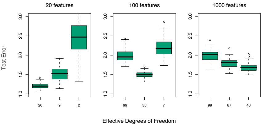
FIGURE 18.1. Test-error results for simulation experiments. Shown are boxplots of the relative test errors over 100 simulations, for three different values of p, the number of features. The relative error is the test error divided by the Bayes error, σ². From left to right, results are shown for ridge regression with three different values of the regularization parameter λ: 0.001, 100 and 1000. The (average) effective degrees of freedom in the fit is indicated below each plot.

variate regression coefficients¹ was 9, 33 and 331, respectively, averaged over the 100 simulation runs. The p = 1000 case is designed to mimic the kind of data that we might see in a high-dimensional genomic or proteomic dataset, for example.

We fit a ridge regression to the data, with three different values for the regularization parameter λ: 0.001, 100, and 1000. When λ = 0.001, this is nearly the same as least squares regression, with a little regularization just to ensure that the problem is non-singular when p>N. Figure 18.1 shows boxplots of the relative test error achieved by the different estimators in each scenario. The corresponding average degrees of freedom used in each ridge-regression fit is indicated (computed using formula (3.50) on page 68²). The degrees of freedom is a more interpretable parameter than λ. We see that ridge regression with λ = 0.001 (20 df) wins when p = 20; λ = 100 (35 df) wins when p = 100, and λ = 1000 (43 df) wins when p = 1000,

Here is an explanation for these results. When p = 20, we fit all the way and we can identify as many of the significant coefficients as possible with

¹We call a regression coefficient significant if ^|βbj/se^{b j | ≥} 2, where ^βˆ^j is the estimated

⁽univariate) coefficient and se^{b j} is its estimated standard error. ²For a fixed value of the regularization parameter ^λ, the degrees of freedom depends on the observed predictor values in each simulation. Hence we compute the average degrees of freedom over simulations.

low bias. When p = 100, we can identify some non-zero coefficients using moderate shrinkage. Finally, when p = 1000, even though there are many nonzero coefficients, we don’t have a hope for finding them and we need to shrink all the way down. As evidence of this, let ^{tj = β}Vj/se^{V j} , where ^βˆ^j is the ridge regression estimate and se^{V j} its estimated standard error. Then using the optimal ridge parameter in each of the three cases, the median value of |t^j | was 2.0, 0.6 and 0.2, and the average number of |t^j | values exceeding 2 was equal to 9.8, 1.2 and 0.0.

Ridge regression with λ = 0.001 successfully exploits the correlation in the features when p<N, but cannot do so when p ≫ N. In the latter case there is not enough information in the relatively small number of samples to efficiently estimate the high-dimensional covariance matrix. In that case, more regularization leads to superior prediction performance.

Thus it is not surprising that the analysis of high-dimensional data requires either modification of procedures designed for the N>p scenario, or entirely new procedures. In this chapter we discuss examples of both kinds of approaches for high dimensional classification and regression; these methods tend to regularize quite heavily, using scientific contextual knowledge to suggest the appropriate form for this regularization. The chapter ends with a discussion of feature selection and multiple testing.

18.2 Diagonal Linear Discriminant Analysis and Nearest Shrunken Centroids

Gene expression arrays are an important new technology in biology, and are discussed in Chapters 1 and 14. The data in our next example form a matrix of 2308 genes (columns) and 63 samples (rows), from a set of microarray experiments. Each expression value is a log-ratio log(R/G). R is the amount of gene-specific RNA in the target sample that hybridizes to a particular (gene-specific) spot on the microarray, and G is the corresponding amount of RNA from a reference sample. The samples arose from small, round blue-cell tumors (SRBCT) found in children, and are classified into four major types: BL (Burkitt lymphoma), EWS (Ewing’s sarcoma), NB (neuroblastoma), and RMS (rhabdomyosarcoma). There is an additional test data set of 20 observations. We will not go into the scientific background here.

Since p ≫ N, we cannot fit a full linear discriminant analysis (LDA) to the data; some sort of regularization is needed. The method we describe here is similar to the methods of Section 4.3.1, but with important modifications that achieve feature selection. The simplest form of regularization assumes that the features are independent within each class, that is, the within-class covariance matrix is diagonal. Despite the fact that features will rarely be independent within a class, when p ≫ N we don’t have

652 18. High-Dimensional Problems: p ≫ N

enough data to estimate their dependencies. The assumption of independence greatly reduces the number of parameters in the model and often results in an effective and interpretable classifier.

Thus we consider the diagonal-covariance LDA rule for classifying the classes. The discriminant score [see (4.12 on page 110] for class k is

\[\delta\_k(x^\*) = -\sum\_{j=1}^p \frac{(x\_j^\* - \bar{x}\_{kj})^2}{s\_j^2} + 2\log \pi\_k. \tag{18.2}\]

Here x^∗ = (x^∗ 1, x^∗ 2,…,x^∗ p)^T is a vector of expression values for a test observation, s^j is the pooled within-class standard deviation of the jth gene, and ¯xkj = # ⁱ∈C^k xij/N^k is the mean of the N^k values for gene j in class k, with C^k being the index set for class k. We call ˜x^k = (¯xk1, x¯k2,… x¯kp)^T the centroid of class k. The first part of (18.2) is simply the (negative) standardized squared distance of x^∗ to the kth centroid. The second part is a correction based on the class prior probability πk, where #^{K k}=1 π^k = 1. The classification rule is then

\[C(x^\*) = \ell \text{ if } \delta\_\ell(x^\*) = \max\_k \delta\_k(x^\*). \tag{18.3}\]

We see that the diagonal LDA classifier is equivalent to a nearest centroid classifier after appropriate standardization. It is also a special case of the naive-Bayes classifier, as described in Section 6.6.3. It assumes that the features in each class have independent Gaussian distributions with the same variance.

The diagonal LDA classifier is often effective in high dimensional settings. It is also called the “independence rule” in Bickel and Levina (2004), who demonstrate theoretically that it will often outperform standard linear discriminant analysis in high-dimensional problems. Here the diagonal LDA classifier yielded five misclassification errors for the 20 test samples. One drawback of the diagonal LDA classifier is that it uses all of the features (genes), and hence is not convenient for interpretation. With further regularization we can do better—both in terms of test error and interpretability.

We would like to regularize in a way that automatically drops out features that are not contributing to the class predictions. We can do this by shrinking the classwise mean toward the overall mean, for each feature separately. The result is a regularized version of the nearest centroid classifier, or equivalently a regularized version of the diagonal-covariance form of LDA. We call the procedure nearest shrunken centroids (NSC).

The shrinkage procedure is defined as follows. Let

\[d\_{kj} = \frac{\bar{x}\_{kj} - \bar{x}\_j}{m\_k(s\_j + s\_0)},\tag{18.4}\]

where ¯x^j is the overall mean for gene j, m^{2 k} = 1/N^k − 1/N and s⁰ is a small positive constant, typically chosen to be the median of the s^j values.

FIGURE 18.2. Soft thresholding function sign(x)(|x|−∆)⁺ is shown in orange, along with the 45◦ line in red.

This constant guards against large dkj values that arise from expression values near zero. With constant within-class variance σ², the variance of the contrast ¯xkj ^{− x}¯^j in the numerator is ^{m2 k}σ², and hence the form of the standardization in the denominator. We shrink the dkj toward zero using soft thresholding

\[d'\_{kj} = \text{sign}(d\_{kj})(|d\_{kj}| - \Delta)\_{+};\tag{18.5}\]

see Figure 18.2. Here ∆ is a parameter to be determined; we used 10-fold cross-validation in the example (see the top panel of Figure 18.4). Each dkj is reduced by an amount ∆ in absolute value, and is set to zero if its absolute value is less than zero. The soft-thresholding function is shown in Figure 18.2; the same thresholding is applied to wavelet coefficients in Section 5.9. An alternative is to use hard thresholding

\[d'\_{kj} = d\_{kj} \cdot I(|d\_{kj}| \ge \Delta);\tag{18.6}\]

we prefer soft-thresholding, as it is a smoother operation and typically works better. The shrunken versions of ¯xkj are then obtained by reversing the transformation in (18.4):

\[ \bar{x}'\_{kj} = \bar{x}\_j + m\_k(s\_j + s\_0)d'\_{kj}.\tag{18.7} \]

We then use the shrunken centroids ¯x′ kj in place of the original ¯xkj in the discriminant score (18.2). The estimator (18.5) can also be viewed as a lasso-style estimator for the class means (Exercise 18.2).

Notice that only the genes that have a nonzero d′ kj for at least one of the classes play a role in the classification rule, and hence the vast majority of genes can often be discarded. In this example, all but 43 genes were discarded, leaving a small interpretable set of genes that characterize each class. Figure 18.3 represents the genes in a heatmap.

Figure 18.4 (top panel) demonstrates the effectiveness of the shrinkage. With no shrinkage we make 5/20 errors on the test data, and several errors

654 18. High-Dimensional Problems: p ≫ N

on the training and CV data. The shrunken centroids achieve zero test errors for a fairly broad band of values for ∆. The bottom panel of Figure 18.4 shows the four centroids for the SRBCT data (gray), relative to the overall centroid. The blue bars are shrunken versions of these centroids, obtained by soft-thresholding the gray bars, using ∆ = 4.3. The discriminant scores (18.2) can be used to construct class probability estimates:

\[ \hat{p}\_k(x^\*) = \frac{e^{\frac{1}{2}\delta\_k(x^\*)}}{\sum\_{\ell=1}^K e^{\frac{1}{2}\delta\_\ell(x^\*)}}.\tag{18.8} \]

These can be used to rate the classifications, or to decide not to classify a particular sample at all.

Note that other forms of feature selection can be used in this setting, including hard thresholding. Fan and Fan (2008) show theoretically the importance of carrying out some kind of feature selection with diagonal linear discriminant analysis in high-dimensional problems.

18.3 Linear Classifiers with Quadratic Regularization

Ramaswamy et al. (2001) present a more difficult microarray classification problem, involving a training set of 144 patients with 14 different types of cancer, and a test set of 54 patients. Gene expression measurements were available for 16, 063 genes.

Table 18.1 shows the prediction results from eight different classification methods. The data from each patient was first standardized to have mean 0 and variance 1; this seems to improve prediction accuracy overall this example, suggesting that the “shape” of each gene-expression profile is important, rather than the absolute expression levels. In each case, the

FIGURE 18.3. Heat-map of the chosen 43 genes. Within each of the horizontal partitions, we have ordered the genes by hierarchical clustering, and similarly for the samples within each vertical partition. Yellow represents over- and blue under-expression.

Number of Genes

FIGURE 18.4. (Top): Error curves for the SRBCT data. Shown are the training, 10-fold cross-validation, and test misclassification errors as the threshold parameter ∆ is varied. The value ∆ = 4.34 is chosen by CV, resulting in a subset of 43 selected genes. (Bottom): Four centroids profiles dkj for the SRBCT data (gray), relative to the overall centroid. Each centroid has 2308 components, and we see considerable noise. The blue bars are shrunken versions d′ kj of these centroids, obtained by soft-thresholding the gray bars, using ∆ = 4.3.

TABLE 18.1. Prediction results for microarray data with 14 cancer classes. Method 1 is described in Section 18.2. Methods 2, 3 and 6 are discussed in Section 18.3, while 4, 7 and 8 are discussed in Section 18.4. Method 5 is described in Section 13.3. The elastic-net penalized multinomial does the best on the test data, but the standard error of each test-error estimate is about 3, so such comparisons are inconclusive.

Methods	CV errors (SE) Out of 144	Test errors Out of 54	Number of Genes Used
1. Nearest shrunken centroids	35 (5.0)	17	6,520
2. L2-penalized discriminant	25 (4.1)	12	16,063
analysis
3. Support vector classifier	26 (4.2)	14	16,063
4. Lasso regression (one vs all)	30.7 (1.8)	12.5	1,429
5. k-nearest neighbors	41 (4.6)	26	16,063
6. L2-penalized multinomial	26 (4.2)	15	16,063
7. L1-penalized multinomial	17 (2.8)	13	269
8. Elastic-net penalized	22 (3.7)	11.8	384
multinomial

regularization parameter has been chosen to minimize the cross-validation error, and the test error at that value of the parameter is shown. When more than one value of the regularization parameter yields the minimal cross-validation error, the average test error at these values is reported.

RDA (regularized discriminant analysis), regularized multinomial logistic regression, and the support vector machine are more complex methods that try to exploit multivariate information in the data. We describe each in turn, as well as a variety of regularization methods, including both L¹ and L² and some in between.

18.3.1 Regularized Discriminant Analysis

Regularized discriminant analysis (RDA) is described in Section 4.3.1. Linear discriminant analysis involves the inversion of a p×p within-covariance matrix. When p ≫ N, this matrix can be huge, has rank at most N<p, and hence is singular. RDA overcomes the singularity issues by regularizing the within-covariance estimate Σˆ . Here we use a version of RDA that shrinks Σˆ towards its diagonal:

\[ \hat{\Delta}(\gamma) = \gamma \hat{\Sigma} + (1 - \gamma) \text{diag}(\hat{\Sigma}), \text{ with } \gamma \in [0, 1]. \tag{18.9} \]

Note that γ = 0 corresponds to diagonal LDA, which is the “no shrinkage” version of nearest shrunken centroids. The form of shrinkage in (18.9) is much like ridge regression (Section 3.4.1), which shrinks the total covariance matrix of the features towards a diagonal (scalar) matrix. In fact, viewing linear discriminant analysis as linear regression with optimal scoring of the categorical response [see (12.58) in Section 12.6], the equivalence becomes more precise.

The computational burden of inverting this large p×p matrix is overcome using the methods discussed in Section 18.3.5. The value of γ was chosen by cross-validation in line 2 of Table 18.1; all values of γ ∈ (0.002, 0.550) gave the same CV and test error. Further development of RDA, including shrinkage of the centroids in addition to the covariance matrix, can be found in Guo et al. (2006).

18.3.2 Logistic Regression with Quadratic Regularization

Logistic regression (Section 4.4) can be modified in a similar way, to deal with the p ≫ N case. With K classes, we use a symmetric version of the multiclass logistic model (4.17) on page 119:

\[\Pr(G = k | X = x) = \frac{\exp(\beta\_{k0} + x^T \beta\_k)}{\sum\_{\ell=1}^K \exp(\beta\_{\ell 0} + x^T \beta\_\ell)}.\tag{18.10}\]

This has K coefficient vectors of log-odds parameters β1, β2,…, βK. We regularize the fitting by maximizing the penalized log-likelihood

\[\max\_{\{\beta\_{0k}, \beta\_k\}\_1^K} \left[ \sum\_{i=1}^N \log \Pr(g\_i | x\_i) - \frac{\lambda}{2} \sum\_{k=1}^K ||\beta\_k||\_2^2 \right]. \tag{18.11}\]

This regularization automatically resolves the redundancy in the parametrization, and forces #^{K k}=1 ^βˆkj = 0, j = 1,…,p (Exercise 18.3). Note that the constant terms βk⁰ are not regularized (and so one should be set to zero). The resulting optimization problem is convex, and can be solved by a Newton algorithm or other numerical techniques. Details are given in Zhu and Hastie (2004). Friedman et al. (2010) provide software for computing the regularization path for the two- and multiclass logistic regression models. Table 18.1, line 6 reports the results for the multiclass logistic regression model, referred to there as “multinomial”. It can be shown (Rosset et al., 2004a) that for separable data, as λ → 0, the regularized (twoclass) logistic regression estimate (renormalized) converges to the maximal margin classifier (Section 12.2). This gives an attractive alternative to the support-vector machine, discussed next, especially in the multiclass case.

18.3.3 The Support Vector Classifier

The support vector classifier is described for the two-class case in Section 12.2. When p>N, it is especially attractive because in general the

658 18. High-Dimensional Problems: p ≫ N

classes are perfectly separable by a hyperplane unless there are identical feature vectors in different classes. Without any regularization the support vector classifier finds the separating hyperplane with the largest margin; that is, the hyperplane yielding the biggest gap between the classes in the training data. Somewhat surprisingly, when p ≫ N the unregularized support vector classifier often works about as well as the best regularized version. Overfitting often does not seem to be a problem, partly because of the insensitivity of misclassification loss.

There are many different methods for generalizing the two-class supportvector classifier to K > 2 classes. In the “one versus one” (ovo) approach, we compute all (^K 2 ) pairwise classifiers. For each test point, the predicted class is the one that wins the most pairwise contests. In the “one versus all” (ova) approach, each class is compared to all of the others in K two-class comparisons. To classify a test point, we compute the confidences (signed distance from the hyperplane) for each of the K classifiers. The winner is the class with the highest confidence. Finally, Vapnik (1998) and Weston and Watkins (1999) suggested (somewhat complex) multiclass criteria which generalize the two-class criterion (12.6).

Tibshirani and Hastie (2007) propose the margin tree classifier, in which support-vector classifiers are used in a binary tree, much as in CART (Chapter 9). The classes are organized in a hierarchical manner, which can be useful for classifying patients into different cancer types, for example.

Line 3 of Table 18.1 shows the results for the support vector classifier using the ova method; Ramaswamy et al. (2001) reported (and we confirmed) that this approach worked best for this problem. The errors are very similar to those in line 6, as we might expect from the comments at the end of the previous section. The error rates are insensitive to the choice of C [the regularization parameter in (12.8) on page 420], for values of C > 0.001. Since p>N, the support vector hyperplane can perfectly separate the training data by setting C = ∞.

18.3.4 Feature Selection

Feature selection is an important scientific requirement for a classifier when p is large. Neither discriminant analysis, logistic regression, nor the supportvector classifier perform feature selection automatically, because all use quadratic regularization. All features have nonzero weights in both models. Ad-hoc methods for feature selection have been proposed, for example, removing genes with small coefficients, and refitting the classifier. This is done in a backward stepwise manner, starting with the smallest weights and moving on to larger weights. This is known as recursive feature elimination (Guyon et al., 2002). It was not successful in this example; Ramaswamy et al. (2001) report, for example, that the accuracy of the support-vector classifier starts to degrade as the number of genes is reduced from the full set of 16, 063. This is rather remarkable, as the number of training samples is only 144. We do not have an explanation for this behavior.

All three methods discussed in this section (RDA, LR and SVM) can be modified to fit nonlinear decision boundaries using kernels. Usually the motivation for such an approach is to increase the model complexity. With p ≫ N the models are already sufficiently complex and overfitting is always a danger. Yet despite the high dimensionality, radial kernels (Section 12.3.3) sometimes deliver superior results in these high dimensional problems. The radial kernel tends to dampen inner products between points far away from each other, which in turn leads to robustness to outliers. This occurs often in high dimensions, and may explain the positive results. We tried a radial kernel with the SVM in Table 18.1, but in this case the performance was inferior.

18.3.5 Computational Shortcuts When p ≫ N

The computational techniques discussed in this section apply to any method that fits a linear model with quadratic regularization on the coefficients. That includes all the methods discussed in this section, and many more. When p>N, the computations can be carried out in an N-dimensional space, rather than p, via the singular value decomposition introduced in Section 14.5. Here is the geometric intuition: just like two points in threedimensional space always lie on a line, N points in p-dimensional space lie in an (N − 1)-dimensional affine subspace.

Given the N × p data matrix X, let

\[\mathbf{X}^{\top} = \mathbf{U} \mathbf{D} \mathbf{V}^{T} \tag{18.12}\]

\[=\begin{array}{c} \mathbf{RV}^T \\ \end{array} \tag{18.13}\]

be the singular-value decomposition (SVD) of X; that is, V is p × N with orthonormal columns, U is N × N orthogonal, and D a diagonal matrix with elements ^{d1 ≥ d2 ≥ dN ≥} 0. The matrix ^R is ^{N × N}, with rows ^rT i .

As a simple example, let’s first consider the estimates from a ridge regression:

\[ \hat{\boldsymbol{\beta}} = (\mathbf{X}^T \mathbf{X} + \lambda \mathbf{I})^{-1} \mathbf{X}^T \mathbf{y}. \tag{18.14} \]

Replacing X by RV^T and after some further manipulations, this can be shown to equal

\[\boldsymbol{\beta}^{\prime} = \mathbf{V} (\mathbf{R}^T \mathbf{R} + \lambda \mathbf{I})^{-1} \mathbf{R}^T \mathbf{y} \tag{18.15}\]

(Exercise 18.4). Thus βˆ = Vˆθ, where ˆθ is the ridge-regression estimate using the N observations (ri, yi), i = 1, 2,…,N. In other words, we can simply reduce the data matrix from X to R, and work with the rows of R. This trick reduces the computational cost from O(p3) to O(pN2) when p>N.

660 18. High-Dimensional Problems: p ≫ N

These results can be generalized to all models that are linear in the parameters and have quadratic penalties. Consider any supervised learning problem where we use a linear function f(X) = β⁰ + X^T β to model a parameter in the conditional distribution of Y |X. We fit the parameters β by minimizing some loss function #^{N i}=1 L(yi, f(xi)) over the data with a quadratic penalty on β. Logistic regression is a useful example to have in mind. Then we have the following simple theorem:

Let f ^∗(ri) = θ⁰ + r^{T i} θ with rⁱ defined in (18.13), and consider the pair of optimization problems:

\[L(\hat{\beta}\_0, \hat{\beta}) \quad = \arg \min\_{\beta\_0, \beta \in \mathbb{R}^p} \sum\_{i=1}^N L(y\_i, \beta\_0 + x\_i^T \beta) + \lambda \beta^T \beta; \tag{18.16}\]

\[\hat{L}(\hat{\theta}\_0, \hat{\theta}) \quad = \text{arg}\min\_{\theta\_0, \theta \in \mathbb{R}^N} \sum\_{i=1}^N L(y\_i, \theta\_0 + r\_i^T \theta) + \lambda \theta^T \theta. \tag{18.17}\]

Then the βˆ⁰ = ˆθ0, and βˆ = Vˆθ.

The theorem says that we can simply replace the p vectors xⁱ by the N-vectors ri, and perform our penalized fit as before, but with far fewer predictors. The N-vector solution ˆθ is then transformed back to the pvector solution via a simple matrix multiplication. This result is part of the statistics folklore, and deserves to be known more widely—see Hastie and Tibshirani (2004) for further details.

Geometrically, we are rotating the features to a coordinate system in which all but the first N coordinates are zero. Such rotations are allowed since the quadratic penalty is invariant under rotations, and linear models are equivariant.

This result can be applied to many of the learning methods discussed in this chapter, such as regularized (multiclass) logistic regression, linear discriminant analysis (Exercise 18.6), and support vector machines. It also applies to neural networks with quadratic regularization (Section 11.5.2). Note, however, that it does not apply to methods such as the lasso, which uses nonquadratic (L1) penalties on the coefficients.

Typically we use cross-validation to select the parameter λ. It can be seen (Exercise 18.12) that we only need to construct R once, on the original data, and use it as the data for each of the CV folds.

The support vector “kernel trick” of Section 12.3.7 exploits the same reduction used in this section, in a slightly different context. Suppose we have at our disposal the ^{N × N} gram (inner-product) matrix ^{K =} XX^T . From (18.12) we have K = UD2U^T , and so K captures the same information as R. Exercise 18.13 shows how we can exploit the ideas in this section to fit a ridged logistic regression with K using its SVD.

18.4 Linear Classifiers with L¹ Regularization

The methods of the previous chapter use an L² penalty to regularize their parameters, just as in ridge regression. All of the estimated coefficients are nonzero, and hence no feature selection is performed. In this section we discuss methods that use L¹ penalties instead, and hence provide automatic feature selection.

Recall the lasso of Section 3.4.2,

\[\min\_{\beta} \frac{1}{2} \sum\_{i=1}^{N} \left( y\_i - \beta\_0 - \sum\_{j=1}^{p} x\_{ij}\beta\_j \right)^2 + \lambda \sum\_{j=1}^{p} |\beta\_j|,\tag{18.18}\]

which we have written in the Lagrange form (3.52). As discussed there, the use of the L¹ penalty causes a subset of the solution coefficients βˆ^j to be exactly zero, for a sufficiently large value of the tuning parameter λ.

In Section 3.8.1 we discussed the LARS algorithm, an efficient procedure for computing the lasso solution for all λ. When p>N (as in this chapter), as λ approaches zero, the lasso fits the training data exactly. In fact, by convex duality one can show that when p>N the number of non-zero coefficients is at most N for all values of λ (Rosset and Zhu, 2007, for example). Thus the lasso provides a (severe) form of feature selection.

Lasso regression can be applied to a two-class classification problem by coding the outcome ±1, and applying a cutoff (usually 0) to the predictions. For more than two classes, there are many possible approaches, including the ova and ovo methods discussed in Section 18.3.3. We tried the ovaapproach on the cancer data in Section 18.3. The results are shown in line (4) of Table 18.1. Its performance is among the best.

A more natural approach for classification problems is to use the lasso penalty to regularize logistic regression. Several implementations have been proposed in the literature, including path algorithms similar to LARS (Park and Hastie, 2007). Because the paths are piecewise smooth but nonlinear, exact methods are slower than the LARS algorithm, and are less feasible when p is large.

Friedman et al. (2010) provide very fast algorithms for fitting L1-penalized logistic and multinomial regression models. They use the symmetric multinomial logistic regression model as in (18.10) in Section 18.3.2, and maximize the penalized log-likelihood

\[\max\_{\{\beta\_{0k}, \beta\_k \in \mathbb{R}^p\}\_1^K} \left[ \sum\_{i=1}^N \log \Pr(g\_i | x\_i) - \lambda \sum\_{k=1}^K \sum\_{j=1}^p |\beta\_{kj}| \right];\tag{18.19}\]

compare with (18.11). Their algorithm computes the exact solution at a pre-chosen sequence of values for λ by cyclical coordinate descent (Section 3.8.6), and exploits the fact that solutions are sparse when p ≫ N,

662 18. High-Dimensional Problems: p ≫ N

as well as the fact that solutions for neighboring values of λ tend to be very similar. This method was used in line (7) of Table 18.1, with the overall tuning parameter λ chosen by cross-validation. The performance was similar to that of the best methods, except here the automatic feature selection chose 269 genes altogether. A similar approach is used in Genkin et al. (2007); although they present their model from a Bayesian point of view, they in fact compute the posterior mode, which solves the penalized maximum-likelihood problem.

FIGURE 18.5. Regularized logistic regression paths for the leukemia data. The left panel is the lasso path, the right panel the elastic-net path with α = 0.8. At the ends of the path (extreme left), there are 19 nonzero coefficients for the lasso, and 39 for the elastic net. The averaging effect of the elastic net results in more non-zero coefficients than the lasso, but with smaller magnitudes.

In genomic applications, there are often strong correlations among the variables; genes tend to operate in molecular pathways. The lasso penalty is somewhat indifferent to the choice among a set of strong but correlated variables (Exercise 3.28). The ridge penalty, on the other hand, tends to shrink the coefficients of correlated variables toward each other (Exercise 3.29 on page 99). The elastic net penalty (Zou and Hastie, 2005) is a compromise, and has the form

\[\sum\_{j=1}^{p} \left( \alpha | \beta\_j | + (1 - \alpha) \beta\_j^2 \right). \tag{18.20}\]

The second term encourages highly correlated features to be averaged, while the first term encourages a sparse solution in the coefficients of these averaged features. The elastic net penalty can be used with any linear model, in particular for regression or classification.

Hence the multinomial problem above with elastic-net penalty becomes

\[\max\_{\{\beta\_{0k}, \beta\_k \in \mathbb{R}^p\}\_1^K} \left[ \sum\_{i=1}^N \log \Pr(g\_i | x\_i) - \lambda \sum\_{k=1}^K \sum\_{j=1}^p \left( \alpha | \beta\_{kj}| + (1 - \alpha) \beta\_{kj}^2 \right) \right]. \tag{18.21}\]

The parameter α determines the mix of the penalties, and is often prechosen on qualitative grounds. The elastic net can yield more that N nonzero coefficients when p>N, a potential advantage over the lasso. Line (8) in Table 18.1 uses this model, with α and λ chosen by cross-validation. We used a sequence of 20 values of α between 0.05 and 1.0, and a 100 values of λ uniform on the log scale covering the entire range. Values of α ∈ [0.75, 0.80] gave the minimum CV error, with values of λ < 0.001 for all tied solutions. Although it has the lowest test error among all methods, the margin is small and not significant. Interestingly, when CV is performed separately for each value of α, a minimum test error of 8.8 is achieved at α = 0.10, but this is not the value chosen in the two-dimensional CV.

FIGURE 18.6. Training, test, and 10-fold cross validation curves for lasso logistic regression on the leukemia data. The left panel shows misclassification errors, the right panel shows deviance.

Figure 18.5 shows the lasso and elastic-net coefficient paths on the twoclass leukemia data (Golub et al., 1999). There are 7129 gene-expression measurements on 38 samples, 27 of them in class ALL (acute lymphocytic leukemia), and 11 in class AML (acute myelogenous leukemia). There is also a test set with 34 samples (20, 14). Since the data are linearly separable, the solution is undefined at λ = 0 (Exercise 18.11), and degrades for very small values of λ. Hence the paths have been truncated as the fitted probabilities approach 0 and 1. There are 19 non-zero coefficients in the left plot, and 39 in the right. Figure 18.6 (left panel) shows the misclassification errors for the lasso logistic regression on the training and test data, as well as for 10-fold cross-validation on the training data. The right panel uses binomial deviance to measure errors, and is much smoother. The small sample sizes lead to considerable sampling variance in these curves, even though individual curves are relatively smooth (see, for example, Figure 7.1 on page 220). Both of these plots suggest that the limiting solution λ ↓ 0 is adequate, leading to 3/34 misclassifications in the test set. The corresponding figures for the elastic net are qualitatively similar and are not shown.

For p ≫ N, the limiting coefficients diverge for all regularized logistic regression models, so in practical software implementations a minimum value for λ > 0 is either explicitly or implicitly set. However, renormalized versions of the coefficients converge, and these limiting solutions can be thought of as interesting alternatives to the linear optimal separating hyperplane (SVM). With α = 0 the limiting solution coincides with the SVM (see end of Section 18.3.2), but all the 7129 genes are selected. With α = 1, the limiting solution coincides with an L¹ separating hyperplane (Rosset et al., 2004a), and includes at most 38 genes. As α decreases from 1, the elastic-net solutions include more genes in the separating hyperplane.

18.4.1 Application of Lasso to Protein Mass Spectroscopy

Protein mass spectrometry has become a popular technology for analyzing the proteins in blood, and can be used to diagnose a disease or understand the processes underlying it.

For each blood serum sample i, we observe the intensity xij for many time of flight values t^j . This intensity is related to the number of particles observed to take approximately t^j time to pass from the emitter to the detector during a cycle of operation of the machine. The time of flight has a known relationship to the mass over charge ratio (m/z) of the constituent proteins in the blood. Hence the identification of a peak in the spectrum at a certain t^j tells us that there is a protein with a corresponding mass and charge. The identity of this protein can then be determined by other means.

Figure 18.7 shows an example taken from Adam et al. (2003). It shows the average spectra for healthy patients and those with prostate cancer. There are 16,898 m/z sites in total, ranging in value from 2000 to 40,000. The full dataset consists of 157 healthy patients and 167 with cancer, and the goal is to find m/z sites that discriminate between the two groups. This is an example of functional data; the predictors can be viewed as a function of m/z. There has been much interest in this problem in the past few years; see e.g. Petricoin et al. (2002).

The data were first standardized (baseline subtraction and normalization), and we restricted attention to m/z values between 2000 and 40,000 (spectra outside of this range were not of interest). We then applied near-

FIGURE 18.7. Protein mass spectrometry data: average profiles from normal and prostate cancer patients.

est shrunken centroids and lasso regression to the data, with the results for both methods shown in Table 18.2.

By fitting harder to the data, the lasso achieves a considerably lower test error rate. However, it may not provide a scientifically useful solution. Ideally, protein mass spectrometry resolves a biological sample into its constituent proteins, and these should appear as peaks in the spectra. The lasso doesn’t treat peaks in any special way, so not surprisingly only some of the non-zero lasso weights were situated near peaks in the spectra. Furthermore, the same protein may yield a peak at slightly different m/z values in different spectra. In order to identify common peaks, some kind of m/z warping is needed from sample to sample.

To address this, we applied a standard peak-extraction algorithm to each spectrum, yielding a total of 5178 peaks in the 217 training spectra. Our idea was to pool the collection of peaks from all patients, and hence construct a set of common peaks. For this purpose, we applied hierarchical clustering to the positions of these peaks along the log m/z axis. We cut the resulting dendrogram horizontally at height log(0.005)³, and computed averages of the peak positions in each resulting cluster. This process yielded 728 common clusters and their corresponding peak centers.

Given these 728 common peaks, we determined which of these were present in each individual spectrum, and if present, the height of the peak. A peak height of zero was assigned if that peak was not found. This produced a 217 × 728 matrix of peak heights as features, which was used in a lasso regression. We scored the test spectra for the same 728 peaks.

³Use of the value 0.005 means that peaks with positions less than 0.5% apart are considered the same peak, a fairly common assumption.

TABLE 18.2. Results for the prostate data example. The standard deviation for the test errors is about 4.5.

Method	Test Errors/108	Number of Sites
1. Nearest shrunken centroids	34	459
2. Lasso	22	113
3. Lasso on peaks	28	35

The prediction results for this application of the lasso to the peaks are shown in the last line of Table 18.2: it does fairly well, but not as well as the lasso on the raw spectra. However, the fitted model may be more useful to the biologist as it yields 35 peak positions for further study. On the other hand, the results suggest that there may be useful discriminatory information between the peaks of the spectra, and the positions of the lasso sites from line (2) of the table also deserve further examination.

18.4.2 The Fused Lasso for Functional Data

In the previous example, the features had a natural order, determined by the mass-to-charge ratio m/z. More generally, we may have functional features xi(t) that are ordered according to some index variable t. We have already discussed several approaches for exploiting such structure.

We can represent xi(t) by their coefficients in a basis of functions in t, such as splines, wavelets or Fourier bases, and then apply a regression using these coefficients as predictors. Equivalently, one can instead represent the coefficients of the original features in these bases. These approaches are described in Section 5.3.

In the classification setting, we discuss the analogous approach of penalized discriminant analysis in Section 12.6. This uses a penalty that explicitly controls the resulting smoothness of the coefficient vector.

The above methods tend to smooth the coefficients uniformly. Here we present a more adaptive strategy that modifies the lasso penalty to take into account the ordering of the features. The fused lasso (Tibshirani et al., 2005) solves

\[\min\_{\beta \in \mathbb{R}^p} \left\{ \sum\_{i=1}^N (y\_i - \beta\_0 - \sum\_{j=1}^p x\_{ij}\beta\_j)^2 + \lambda\_1 \sum\_{j=1}^p |\beta\_j| + \lambda\_2 \sum\_{j=1}^{p-1} |\beta\_{j+1} - \beta\_j| \right\}. \tag{18.22}\]

This criterion is strictly convex in β, so a unique solution exists. The first penalty encourages the solution to be sparse, while the second encourages it to be smooth in the index j.

The difference penalty in (18.22) assumes an uniformly spaced index j. If instead the underlying index variable t has nonuniform values t^j , a natural generalization of (18.22) would be based on divided differences

FIGURE 18.8. Fused lasso applied to CGH data. Each point represents the copy-number of a gene in a tumor sample, relative to that of a control (on the log base-2 scale).

\[ \lambda\_2 \sum\_{j=1}^{p-1} \frac{|\beta\_{j+1} - \beta\_j|}{|t\_{j+1} - t\_j|}. \tag{18.23} \]

This amounts to having a penalty modifier for each of the terms in the series.

A particularly useful special case arises when the predictor matrix X = I^N , the N × N identity matrix. This is a special case of the fused lasso, used to approximate a sequence {yi}^{N 1} . The fused lasso signal approximator solves

\[\min\_{\beta \in \mathbb{R}^N} \left\{ \sum\_{i=1}^N (y\_i - \beta\_0 - \beta\_i)^2 + \lambda\_1 \sum\_{i=1}^N |\beta\_i| + \lambda\_2 \sum\_{i=1}^{N-1} |\beta\_{i+1} - \beta\_i| \right\}. \tag{18.24}\]

Figure 18.8 shows an example taken from Tibshirani and Wang (2007). The data in the panel come from a Comparative Genomic Hybridization (CGH) array, measuring the approximate log (base-two) ratio of the number of copies of each gene in a tumor sample, as compared to a normal sample. The horizontal axis represents the chromosomal location of each gene. The idea is that in cancer cells, genes are often amplified (duplicated) or deleted, and it is of interest to detect these events. Furthermore, these events tend to occur in contiguous regions. The smoothed signal estimate from the fused lasso signal approximator is shown in dark red (with appropriately chosen values for λ¹ and λ2). The significantly nonzero regions can be used to detect locations of gains and losses of genes in the tumor.

There is also a two-dimensional version of the fused lasso, in which the parameters are laid out in a grid of pixels, and a penalty is applied to the first differences to the left, right, above and below the target pixel. This can be useful for denoising or classifying images. Friedman et al. (2007) develop fast generalized coordinate descent algorithms for the one- and two-dimensional fused lasso.

18.5 Classification When Features are Unavailable

In some applications the objects under study are more abstract in nature, and it is not obvious how to define a feature vector. As long as we can fill in an N ×N proximity matrix of similarities between pairs of objects in our database, it turns out we can put to use many of the classifiers in our arsenal by interpreting the proximities as inner-products. Protein structures fall into this category, and we explore an example in Section 18.5.1 below.

In other applications, such as document classification, feature vectors are available but can be extremely high-dimensional. Here we may not wish to compute with such high-dimensional data, but rather store the innerproducts between pairs of documents. Often these inner-products can be approximated by sampling techniques.

Pairwise distances serve a similar purpose, because they can be turned into centered inner-products. Proximity matrices are discussed in more detail in Chapter 14.

18.5.1 Example: String Kernels and Protein Classification

An important problem in computational biology is to classify proteins into functional and structural classes based on their sequence similarities. Protein molecules are strings of amino acids, differing in both length and composition. In the example we consider, the lengths vary between 75–160 amino-acid molecules, each of which can be one of 20 different types, labeled using letters. Here are two examples, of length 110 and 153, respectively:

IPTSALVKETLALLSTHRTLLIANETLRIPVPVHKNHQLCTEEIFQGIGTLESQTVQGGTV ERLFKNLSLIKKYIDGQKKKCGEERRRVNQFLDYLQEFLGVMNTEWI

PHRRDLCSRSIWLARKIRSDLTALTESYVKHQGLWSELTEAERLQENLQAYRTFHVLLA RLLEDQQVHFTPTEGDFHQAIHTLLLQVAAFAYQIEELMILLEYKIPRNEADGMLFEKK LWGLKVLQELSQWTVRSIHDLRFISSHQTGIP

There have been many proposals for measuring the similarity between a pair of protein molecules. Here we focus on a measure based on the count of matching substrings (Leslie et al., 2004), such as the LQE above.

To construct our features, we count the number of times that a given sequence of length m occurs in our string, and we compute this number for all possible sequences of length m. Formally, for a string x, we define a feature map

\[\Phi\_m(x) = \{\phi\_a(x)\}\_{a \in \mathcal{A}\_m} \tag{18.25}\]

where A^m is the set of subsequences of length m, and φa(x) is the number of times that “a” occurs in our string x. Using this, we define the inner product

\[K\_m(x\_1, x\_2) = \langle \Phi\_m(x\_1), \Phi\_m(x\_2) \rangle,\tag{18.26}\]

which measures the similarity between the two strings x1, x2. This can be used to drive, for example, a support vector classifier for classifying strings into different protein classes.

Now the number of possible sequences ^a is |Am^| = 20m, which can be very large for moderate m, and the vast majority of the subsequences do not match the strings in our training set. It turns out that we can compute the N × N inner-product matrix or string kernel K^m (18.26) efficiently using tree-structures, without actually computing the individual vectors. This methodology, and the data to follow, come from Leslie et al. (2004).⁴

The data consist of 1708 proteins in two classes— negative (1663) and positive (45). The two examples above, which we will call “x1” and “x2”, are from this set. We have marked the occurrences of subsequence LQE, which appears in both proteins. There are 20³ possible subsequences, so Φ3(x) will be a vector of length 8000. For this example φLQE(x1) = 1 and φLQE(x2) = 2.

Using software from Leslie et al. (2004), we computed the string kernel for m = 4, which was then used in a support vector classifier to find the maximal margin solution in this 20⁴ = 160, 000-dimensional feature space. We used 10-fold cross-validation to compute the SVM predictions on all of the training data. The orange curve in Figure 18.9 shows the cross-validated ROC curve for the support vector classifier, computed by varying the cutpoint on the real-valued predictions from the cross-validated support vector classifier. The area under the curve is 0.84. Leslie et al. (2004) show that the string kernel method is competitive with, but perhaps not as accurate as, more specialized methods for protein string matching.

Many other classifiers can be computed using only the information in the kernel matrix; some details are given in the next section. The results for the nearest centroid classifier (green), and distance-weighted one-nearest neighbors (blue) are shown in Figure 18.9. Their performance is similar to that of the support vector classifier.

⁴We thank Christina Leslie for her help and for providing the data, which is available on our book website.

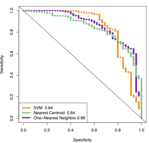
ROC Curves for String Kernel

FIGURE 18.9. Cross-validated ROC curves for protein example using the string kernel. The numbers next to each method in the legend give the area under the curve, an overall measure of accuracy. The SVM achieves better sensitivities than the other two, which achieve better specificities.

18.5.2 Classification and Other Models Using Inner-Product Kernels and Pairwise Distances

There are a number of other classifiers, besides the support-vector machine, that can be implemented using only inner-product matrices. This also implies they can be “kernelized” like the SVM.

An obvious example is nearest-neighbor classification, since we can transform pairwise inner-products to pairwise distances:

\[\left| \left| \left| x\_i - x\_{i'} \right| \right| ^2 = \langle x\_i, x\_i \rangle + \langle x\_{i'}, x\_{i'} \rangle - 2 \langle x\_i, x\_{i'} \rangle. \tag{18.27}\]

A variation of 1-NN classification is used in Figure 18.9, which produces a continuous discriminant score needed to construct a ROC curve. This distance-weighted 1-NN makes use of the distance of a test points to the closest member of each class; see Exercise 18.14.

Nearest-centroid classification follows easily as well. For training pairs (xi, gi), i = 1,…,N, a test point x0, and class centroids ¯xk, k = 1,…,K we can write

\[||x\_0 - \bar{x}\_k||^2 = \langle x\_0, x\_0 \rangle - \frac{2}{N\_k} \sum\_{g\_i=k} \langle x\_0, x\_i \rangle + \frac{1}{N\_k^2} \sum\_{g\_i=k} \sum\_{g\_{i'}=k} \langle x\_i, x\_{i'} \rangle,\tag{18.28}\]

Hence we can compute the distance of the test point to each of the centroids, and perform nearest centroid classification. This also implies that methods like K-means clustering can also be implemented, using only the inner products of the data points.

Logistic and multinomial regression with quadratic regularization can also be implemented with inner-product kernels; see Section 12.3.3 and Exercise 18.13. Exercise 12.10 derives linear discriminant analysis using an inner-product kernel.

Principal components can be computed using inner-product kernels as well; since this is frequently useful, we give some details. Suppose first that we have a centered data matrix X, and let X = UDV^T be its SVD (18.12). Then Z = UD is the matrix of principal component variables (see Section 14.5.1). But if K = XX^T , then it follows that K = UD2U^T , and hence we can compute Z from the eigen decomposition of K. If X is not centered, then we can center it using ^X˜ = (^{I − M})X, where ^{M = 1 N} 11^T is the mean operator. Thus we compute the eigenvectors of the doublecentered kernel (I − M)K(I − M) for the principal components from an uncentered inner-product matrix. Exercise 18.15 explores this further, and Section 14.5.4 discusses in more detail kernel PCA for general kernels, such as the radial kernel used in SVMs.

If instead we had available only the pairwise (squared) Euclidean distances between observations,

\[ \Delta\_{ii'}^2 = ||x\_i - x\_{i'}||^2,\tag{18.29} \]

it turns out we can do all of the above as well. The trick is to convert the pairwise distances to centered inner-products, and then proceed as before. We write

\[ \Delta\_{ii'}^2 = ||x\_i - \bar{x}||^2 + ||x\_{i'} - \bar{x}||^2 - 2\langle x\_i - \bar{x}, x\_{i'} - \bar{x} \rangle. \tag{18.30} \]

Defining ^{B =} {−∆² ii′/2}, we double center B:

\[ \tilde{\mathbf{K}} = (\mathbf{I} - \mathbf{M})\mathbf{B}(\mathbf{I} - \mathbf{M});\tag{18.31} \]

it is easy to check that ^K˜ii′ ⁼ ⟨x^{i −} x, x ¯ ⁱ′ ^{− x}¯⟩, the centered inner-product matrix.

Distances and inner-products also allow us to compute the medoid in each class—the observation with smallest average distance to other observations in that class. This can be used for classification (closest medoids), as well as to drive k-medoids clustering (Section 14.3.10). With abstract data objects like proteins, medoids have a practical advantage over means. The medoid is one of the training examples, and can be displayed. We tried closest medoids in the example in the next section (see Table 18.3), and its performance is disappointing.

It is useful to consider what we cannot do with inner-product kernels and distances:

TABLE 18.3. Cross-validated error rates for the abstracts example. The nearest shrunken centroids ended up using no-shrinkage, but does use a word-by-word standardization (section 18.2). This standardization gives it a distinct advantage over the other methods.

	Method	CV Error (SE)
1.	Nearest shrunken centroids	0.17 (0.05)
2.	SVM	0.23 (0.06)
3.	Nearest medoids	0.65 (0.07)
4.	1-NN	0.44 (0.07)
5.	Nearest centroids	0.29 (0.07)

• We cannot standardize the variables; standardization significantly improves performance in the example in the next section.
• We cannot assess directly the contributions of individual variables. In particular, we cannot perform individual t-tests, fit the nearest shrunken centroids model, or fit any model that uses the lasso penalty.
• We cannot separate the good variables from the noise: all variables get an equal say. If, as is often the case, the ratio of relevant to irrelevant variables is small, methods that use kernels are not likely to work as well as methods that do feature selection.

18.5.3 Example: Abstracts Classification

This somewhat whimsical example serves to illustrate a limitation of kernel approaches. We collected the abstracts from 48 papers, 16 each from Bradley Efron (BE), Trevor Hastie and Rob Tibshirani (HT) (frequent coauthors), and Jerome Friedman (JF). We extracted all unique words from these abstracts, and defined features xij to be the number of times word j appears in abstract i. This is the so-called bag of words representation. Quotations, parentheses and special characters were first removed from the abstracts, and all characters were converted to lower case. We also removed the word “we”, which could unfairly discriminate HT abstracts from the others.

There were 4492 total words, of which p = 1310 were unique. We sought to classify the documents into BE, HT or JF on the basis of the features xij . Although it is artificial, this example allows us to assess the possible degradation in performance if information specific to the raw features is not used.

We first applied the nearest shrunken centroid classifier to the data, using 10-fold cross-validation. It essentially chose no shrinkage, and so used all the features; see the first line of Table 18.3. The error rate is 17%; the number of features can be reduced to about 500 without much loss in accuracy. Note that the nearest shrunken classifier requires the raw feature matrix X in order to standardize the features individually. Figure 18.10 shows the

FIGURE 18.10. Abstracts example: top 20 scores from nearest shrunken centroids. Each score is the standardized difference in frequency for the word in the given class (BE, HT or JF) versus all classes. Thus a positive score (to the right of the vertical grey zero lines) indicates a higher frequency in that class; a negative score indicates a lower relative frequency.

top 20 discriminating words, with a positive score indicating that a word appears more in that class than in the other classes.

Some of these terms make sense: for example “frequentist” and “Bayesian” reflect Efron’s greater emphasis on statistical inference. However, many others are surprising, and reflect personal writing styles: for example, Friedman’s use of “presented” and HT’s use of “propose”.

We then applied the support vector classifier with linear kernel and no regularization, using the “all pairs” (ovo) method to handle the three classes (regularization of the SVM did not improve its performance). The result is shown in Table 18.3. It does somewhat worse than the nearest shrunken centroid classifier.

As mentioned, the first line of Table 18.3 represents nearest shrunken centroids (with no shrinkage). Denote by s^j the pooled within-class standard deviation for feature j, and s⁰ the median of the s^j values. Then line (1) also corresponds to nearest centroid classification, after first standardizing each feature by s^j + s⁰ [recall (18.4) on page 652].

Line (3) shows that the performance of nearest medoids is very poor, something which surprised us. It is perhaps due to the small sample sizes

674 18. High-Dimensional Problems: p ≫ N

and high dimensions, with medoids having much higher variance than means. The performance of the one-nearest neighbor classifier is also poor.

The performance of the nearest centroid classifier is also shown in Table 18.3 in line (5): it is better than nearest medoids, but worse than that of nearest shrunken centroids, even with no shrinkage. The difference seems to be the standardization of each feature that is done in nearest shrunken centroids. This standardization is important here, and requires access to the individual feature values. Nearest centroids uses a spherical metric, and relies on the fact that the features are in similar units. The support vector machine estimates a linear combination of the features and can better deal with unstandardized features.

18.6 High-Dimensional Regression: Supervised Principal Components

In this section we describe a simple approach to regression and generalized regression that is especially useful when p ≫ N. We illustrate the method on another microarray data example. The data is taken from Rosenwald et al. (2002) and consists of 240 samples from patients with diffuse large B-cell lymphoma (DLBCL), with gene expression measurements for 7399 genes. The outcome is survival time, either observed or right censored. We randomly divided the lymphoma samples into a training set of size 160 and a test set of size 80.

Although supervised principal components is useful for linear regression, its most interesting applications may be in survival studies, which is the focus of this example.

We have not yet discussed regression with censored survival data in this book; it represents a generalized form of regression in which the outcome variable (survival time) is only partly observed for some individuals. Suppose for example we carry out a medical study that lasts for 365 days, and for simplicity all subjects are recruited on day one. We might observe one individual to die 200 days after the start of the study. Another individual might still be alive at 365 days when the study ends. This individual is said to be “right censored” at 365 days. We know only that he or she lived at least 365 days. Although we do not know how long past 365 days the individual actually lived, the censored observation is still informative. This is illustrated in Figure 18.11. Figure 18.12 shows the survival curve estimated by the Kaplan–Meier method for the 80 patients in the test set. See for example Kalbfleisch and Prentice (1980) for a description of the Kaplan–Meier method.

Our objective in this example is to find a set of features (genes) that can predict the survival of an independent set of patients. This could be

FIGURE 18.11. Censored survival data. For illustration there are four patients. The first and third patients die before the study ends. The second patient is alive at the end of the study (365 days), while the fourth patient is lost to follow-up before the study ends. For example, this patient might have moved out of the country. The survival times for patients two and four are said to be “censored.”

FIGURE 18.12. Lymphoma data. The Kaplan–Meier estimate of the survival function for the 80 patients in the test set, along with one-standard-error curves. The curve estimates the probability of surviving past t months. The ticks indicate censored observations.

probability density

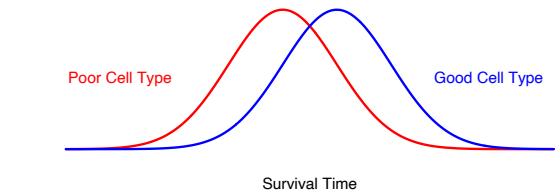
FIGURE 18.13. Underlying conceptual model for supervised principal components. There are two cell types, and patients with the good cell type live longer on the average. Supervised principal components estimate the cell type, by averaging the expression of genes that reflect it.

useful as a prognostic indicator to aid in choosing treatments, or to help understand the biological basis for the disease.

The underlying conceptual model for supervised principal components is shown in Figure 18.13. We imagine that there are two cell types, and patients with the good cell type live longer on the average. However there is considerable overlap in the two sets of survival times. We might think of survival time as a “noisy surrogate” for cell type. A fully supervised approach would give the most weight to those genes having the strongest relationship with survival. These genes are partially, but not perfectly, related to cell type. If we could instead discover the underlying cell types of the patients, often reflected by a sizable signature of genes acting together in pathways, then we might do a better job of predicting patient survival.

Although the cell type in Figure 18.13 is discrete, it is useful to imagine a continuous cell type, define by some linear combination of the features. We will estimate the cell type as a continuous quantity, and then discretize it for display and interpretation.

How can we find the linear combination that defines the important underlying cell types? Principal components analysis (Section 14.5) is an effective method for finding linear combinations of features that exhibit large variation in a dataset. But what we seek here are linear combinations with both high variance and significant correlation with the outcome. The lower right panel of Figure 18.14 shows the result of applying standard principal components in this example; the leading component does not correlate strongly with survival (details are given in the figure caption).

Hence we want to encourage principal component analysis to find linear combinations of features that have high correlation with the outcome. To do this, we restrict attention to features which by themselves have a sizable correlation with the outcome. This is summarized in the supervised principal components Algorithm 18.1, and illustrated in Figure 18.14.

The details in steps (1) and (2b) will depend on the type of outcome variable. For a standard regression problem, we use the univariate linear least squares coefficients in step (1) and a linear least squares model in

FIGURE 18.14. Supervised principal components on the lymphoma data. The left panel shows a heatmap of a subset of the gene-expression training data. The rows are ordered by the magnitude of the univariate Cox-score, shown in the middle vertical column. The top 50 and bottom 50 genes are shown. The supervised principal component uses the top 27 genes (chosen by 10-fold CV). It is represented by the bar at the top of the heatmap, and is used to order the columns of the expression matrix. In addition, each row is multiplied by the sign of the Cox-score. The middle panel on the right shows the survival curves on the test data when we create a low and high group by splitting this supervised PC at zero (training data mean). The curves are well separated, as indicated by the p-value for the log-rank test. The top panel does the same, using the top-scoring gene on the training data. The curves are somewhat separated, but not significantly. The bottom panel uses the first principal component on all the genes, and the separation is also poor. Each of the top genes can be interpreted as noisy surrogates for a latent underlying cell-type characteristic, and supervised principal components uses them all to estimate this latent factor.

Algorithm 18.1 Supervised Principal Components.

• 1. Compute the standardized univariate regression coefficients for the outcome as a function of each feature separately.
• 2. For each value of the threshold θ from the list 0 ≤ θ¹ < θ² < ··· < θK:
  • 1. Form a reduced data matrix consisting of only those features whose univariate coefficient exceeds θ in absolute value, and compute the first m principal components of this matrix.
  • 2. Use these principal components in a regression model to predict the outcome.
• 3. Pick θ (and m) by cross-validation.

step (2b). For survival problems, Cox’s proportional hazards regression model is widely used; hence we use the score test from this model in step (1) and the multivariate Cox model in step (2b). The details are not essential for understanding the basic method; they may be found in Bair et al. (2006).

Figure 18.14 shows the results of supervised principal components in this example. We used a Cox-score cutoff of 3.53, yielding 27 genes, where the value 3.53 was found through 10-fold cross-validation. We then computed the first principal component (m = 1) using just this subset of the data, as well as its value for each of the test observations. We included this as a quantitative predictor in a Cox regression model, and its likelihood-ratio significance was p = 0.005. When dichotomized (using the mean score on the training data as a threshold), it clearly separates the patients in the test set into low and high risk groups (middle-right panel of Figure 18.14, p = 0.006).

The top-right panel of Figure 18.14 uses the top scoring gene (dichotomized) alone as a predictor of survival. It is not significant on the test set. Likewise, the lower-right panel shows the dichotomized principal component using all the training data, which is also not significant.

Our procedure allows m > 1 principal components in step (2a). However, the supervision in step (1) encourages the principal components to align with the outcome, and thus in most cases only the first or first few components tend to be useful for prediction. In the mathematical development below, we consider only the first component, but extensions to more than one component can be derived in a similar way.

18.6.1 Connection to Latent-Variable Modeling

A formal connection between supervised principal components and the underlying cell type model (Figure 18.13) can be seen through a latent variable model for the data. Suppose we have a response variable Y which is related to an underlying latent variable U by a linear model

\[Y = \beta\_0 + \beta\_1 U + \varepsilon. \tag{18.32}\]

In addition, we have measurements on a set of features X^j indexed by j ∈ P (for pathway), for which

\[X\_j = \alpha\_{0j} + \alpha\_{1j}U + \epsilon\_j, \quad j \in \mathcal{P}.\tag{18.33}\]

The errors ε and ϵ^j are assumed to have mean zero and are independent of all other random variables in their respective models.

We also have many additional features Xk, k ̸∈ P which are independent of U. We would like to identify P, estimate U, and hence fit the prediction model (18.32). This is a special case of a latent-structure model, or single-component factor-analysis model (Mardia et al., 1979, see also Section 14.7). The latent factor U is a continuous version of the cell type conceptualized in Figure 18.13.

The supervised principal component algorithm can be seen as a method for fitting this model:

• The screening step (1) estimates the set P.
• Given PV, the largest principal component in step (2a) estimates the latent factor U.
• Finally, the regression fit in step (2b) estimates the coefficient in model (18.32).

Step (1) is natural, since on average the regression coefficient is nonzero only if α1^j is non-zero. Hence this step should select the features j ∈ P. Step (2a) is natural if we assume that the errors ϵ^j have a Gaussian distribution, with the same variance. In this case the principal component is the maximum likelihood estimate for the single factor model (Mardia et al., 1979). The regression in (2b) is an obvious final step.

Suppose there are a total of p features, with p¹ features in the relevant set P. Then if p and p¹ grow but p¹ is small relative to p, one can show (under reasonable conditions) that the leading supervised principal component is consistent for the underlying latent factor. The usual leading principal component may not be consistent, since it can be contaminated by the presence of a large number of “noise” features.

Finally, suppose that the threshold used in step (1) of the supervised principal component procedure yields a large number of features for computation of the principal component. Then for interpretational purposes, as well as for practical uses, we would like some way of finding a reduced a set of features that approximates the model. Pre-conditioning (Section 18.6.3) is one way of doing this.

18.6.2 Relationship with Partial Least Squares

Supervised principal components is closely related to partial least squares regression (Section 3.5.2). Bair et al. (2006) found that the key to the good performance of supervised principal components was the filtering out of noisy features in step (2a). Partial least squares (Section 3.5.2) downweights noisy features, but does not throw them away; as a result a large number of noisy features can contaminate the predictions. However, a modification of the partial least squares procedure has been proposed that has a similar flavor to supervised principal components [Brown et al. (1991),Nadler and Coifman (2005), for example]. We select the features as in steps (1) and (2a) of supervised principal components, but then apply PLS (rather than principal components) to these features. For our current discussion, we call this “thresholded PLS.”

Thresholded PLS can be viewed as a noisy version of supervised principal components, and hence we might not expect it to work as well in practice. Assume the variables are all standardized. The first PLS variate has the form

\[\mathbf{z} = \sum\_{j \in \mathcal{P}} \langle \mathbf{y}, \mathbf{x}\_j \rangle \mathbf{x}\_j,\tag{18.34}\]

and can be thought of as an estimate of the latent factor U in model (18.33). In contrast, the supervised principal components direction uˆ satisfies

\[ \hat{\mathbf{u}} = \frac{1}{d^2} \sum\_{j \in \mathcal{P}} \langle \hat{\mathbf{u}}, \mathbf{x}\_j \rangle \mathbf{x}\_j,\tag{18.35} \]

where d is the leading singular value of X^P . This follows from the definition of the leading principal component. Hence thresholded PLS uses weights which are the inner product of y with each of the features, while supervised principal components uses the features to derive a “self-consistent” estimate uˆ. Since many features contribute to the estimate uˆ, rather than just the single outcome y, we can expect uˆ to be less noisy than z. In fact, if there are p¹ features in the set P, and N, p and p¹ go to infinity with p1/N → 0, then it can be shown using the techniques in Bair et al. (2006) that

\[\begin{array}{rcl} \mathbf{z} & = & \mathbf{u} + O\_p(1) \\ \hat{\mathbf{u}} & = & \mathbf{u} + O\_p(\sqrt{p\_1/N}), \end{array} \tag{18.36}\]

where u is the true (unobservable) latent variable in the model (18.32), (18.33).

We now present a simulation example to compare the methods numerically. There are N = 100 samples and p = 5000 genes. We generated the data as follows:

FIGURE 18.15. Heatmap of the outcome (left column) and first 500 genes from a realization from model (18.37). The genes are in the columns, and the samples are in the rows.

\[\begin{array}{rclrcl} x\_{ij} &=& \begin{cases} 3+\epsilon\_{ij} & \text{if } i \le 50, & j = 1, \dots, 50 \\ 4+\epsilon\_{ij} & \text{if } i > 50 \\ 1.5+\epsilon\_{ij} & \text{if } 1 \le i \le 25 \text{ or } 51 \le i \le 75 \\ 5.5+\epsilon\_{ij} & \text{if } 26 \le i \le 50 \text{ or } 76 \le i \le 100 \\ x\_{ij} &=& \epsilon\_{ij} \\ y\_{i} &=& 2 \cdot \frac{1}{50} \sum\_{j=1}^{50} x\_{ij} + \varepsilon\_{i} \end{array} & j = 251, \dots, 5000 \end{array}\]

(18.37)

where ϵij and εⁱ are independent normal random variables with mean 0 and standard deviations 1 and 1.5, respectively. Thus in the first 50 genes, there is an average difference of 1 unit between samples 1–50 and 51–100, and this difference correlates with the outcome y. The next 200 genes have a large average difference of 4 units between samples (1–25, 51–75) and (26–50, 76–100), but this difference is uncorrelated with the outcome. The rest of the genes are noise. Figure 18.15 shows a heatmap of a typical realization, with the outcome at the left, and the first 500 genes to the right.

We generated 100 simulations from this model, and summarize the test error results in Figure 18.16. The test errors of principal components and partial least squares are shown at the right of the plot; both are badly affected by the noisy features in the data. Supervised principal components and thresholded PLS work best over a wide range of the number of selected features, with the former showing consistently lower test errors.

While this example seems “tailor-made” for supervised principal components, its good performance seems to hold in other simulated and real datasets (Bair et al., 2006).

18.6.3 Pre-Conditioning for Feature Selection

Supervised principal components can yield lower test errors than competing methods, as shown in Figure 18.16. However, it does not always produce a sparse model involving only a small number of features (genes). Even if the thresholding in Step (1) of the algorithm yields a relatively small number

FIGURE 18.16. Root mean squared test error (± one standard error), for supervised principal components and thresholded PLS on 100 realizations from model (18.37). All methods use one component, and the errors are relative to the noise standard deviation (the Bayes error is 1.0). For both methods, different values for the filtering threshold were tried and the number of features retained is shown on the horizontal axis. The extreme right points correspond to regular principal components and partial least squares, using all the genes.

of features, it may be that some of the omitted features have sizable inner products with the supervised principal component (and could act as a good surrogate). In addition, highly correlated features will tend to be chosen together, and there may be great deal of redundancy in the set of selected features.

The lasso (Sections 18.4 and 3.4.2), on the other hand, produces a sparse model from the data. How do the test errors of the two methods compare on the simulated example of the last section? Figure 18.17 shows the test errors for one realization from model (18.37) for the lasso, supervised principal components, and the pre-conditioned lasso (described below).

We see that supervised principal components (orange curve) reaches its lowest error when about 50 features are included in the model, which is the correct number for the simulation. Although a linear model in the first 50 features is optimal, the lasso (green) is adversely affected by the large number of noisy features, and starts overfitting when far fewer are in the model.

Can we get the low test error of supervised principal components along with the sparsity of the lasso? This is the goal of pre-conditioning (Paul et al., 2008). In this approach, one first computes the supervised principal component predictor ˆyⁱ for each observation in the training set (with the

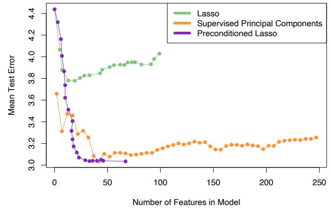
FIGURE 18.17. Test errors for the lasso, supervised principal components, and pre-conditioned lasso, for one realization from model (18.37). Each model is indexed by the number of non-zero features. The supervised principal component path is truncated at 250 features. The lasso self-truncates at 100, the sample size (see Section 18.4). In this case, the pre-conditioned lasso achieves the lowest error with about 25 features.

threshold selected by cross-validation). Then we apply the lasso with ˆyⁱ as the outcome variable, in place of the usual outcome yi. All features are used in the lasso fit, not just those that were retained in the thresholding step in supervised principal components. The idea is that by first denoising the outcome variable, the lasso should not be as adversely affected by the large number of noise features. Figure 18.17 shows that pre-conditioning (purple curve) has been successful here, yielding much lower test error than the usual lasso, and as low (in this case) as for supervised principal components. It also can achieve this using less features. The usual lasso, applied to the raw outcome, starts to overfit more quickly than the pre-conditioned version. Overfitting is not a problem, since the outcome variable has been denoised. We usually select the tuning parameter for the pre-conditioned lasso on more subjective grounds, like parsimony.

Pre-conditioning can be applied in a variety of settings, using initial estimates other than supervised principal components and post-processors other than the lasso. More details may be found in Paul et al. (2008).

18.7 Feature Assessment and the Multiple-Testing Problem

In the first part of this chapter we discuss prediction models in the p ≫ N setting. Here we consider the more basic problem of assessing the significance of each of the p features. Consider the protein mass spectrometry example of Section 18.4.1. In that problem, the scientist might not be interested in predicting whether a given patient has prostate cancer. Rather the goal might be to identify proteins whose abundance differs between normal and cancer samples, in order to enhance understanding of the disease and suggest targets for drug development. Thus our goal is to assess the significance of individual features. This assessment is usually done without the use of a multivariate predictive model like those in the first part of this chapter. The feature assessment problem moves our focus from prediction to the traditional statistical topic of multiple hypothesis testing. For the remainder of this chapter we will use M instead of p to denote the number of features, since we will frequently be referring to p-values.

TABLE 18.4. Subset of the 12, 625 genes from microarray study of radiation sensitivity. There are a total of 44 samples in the normal group and 14 in the radiation sensitive group; we only show three samples from each group.

	Normal				Radiation Sensitive
Gene 1	7.85	29.74	29.50		17.20	-50.75	-18.89
Gene 2	15.44	2.70	19.37		6.57	-7.41	79.18
Gene 3	-1.79	15.52	-3.13		-8.32	12.64	4.75
Gene 4	-11.74	22.35	-36.11		-52.17	7.24	-2.32
Gene 12,625	-14.09	32.77	57.78		-32.84	24.09	-101.44

Consider, for example, the microarray data in Table 18.4, taken from a study on the sensitivity of cancer patients to ionizing radiation treatment (Rieger et al., 2004). Each row consists of the expression of genes in 58 patient samples: 44 samples were from patients with a normal reaction, and 14 from patients who had a severe reaction to radiation. The measurements were made on oligo-nucleotide microarrays. The object of the experiment was to find genes whose expression was different in the radiation sensitive group of patients. There are M = 12, 625 genes altogether; the table shows the data for some of the genes and samples for illustration.

To identify informative genes, we construct a two-sample t-statistic for each gene.

\[t\_j = \frac{\bar{x}\_{2j} - \bar{x}\_{1j}}{\text{se}\_j},\tag{18.38}\]

where ¯xkj = # ⁱ∈C^ℓ xij/Nℓ. Here C^ℓ are the indices of the N^ℓ samples in group ℓ, where ℓ = 1 is the normal group and ℓ = 2 is the sensitive group. The quantity se^j is the pooled within-group standard error for gene j:

FIGURE 18.18. Radiation sensitivity microarray example. A histogram of the 12, 625 t-statistics comparing the radiation-sensitive versus insensitive groups. Overlaid in blue is the histogram of the t-statistics from 1000 permutations of the sample labels.

\[\text{res}\_{j} = \hat{\sigma}\_{j} \sqrt{\frac{1}{N\_{1}} + \frac{1}{N\_{2}}}; \ \hat{\sigma}\_{j}^{2} = \frac{1}{N\_{1} + N\_{2} - 2} \left( \sum\_{i \in C\_{1}} (x\_{ij} - \bar{x}\_{1j})^{2} + \sum\_{i \in C\_{2}} (x\_{ij} - \bar{x}\_{2j})^{2} \right) . \tag{18.39}\]

A histogram of the 12,625 t-statistics is shown in orange in Figure 18.18, ranging in value from −4.7 to 5.0. If the t^j values were normally distributed we could consider any value greater than two in absolute value to be significantly large. This would correspond to a significance level of about 5%. Here there are 1189 genes with |t^j | ≥ 2. However with 12,625 genes we would expect many large values to occur by chance, even if the grouping is unrelated to any gene. For example, if the genes were independent (which they are surely not), the number of falsely significant genes would have a binomial distribution with mean 12, 625 · 0.05 = 631.3 and standard deviation 24.5; the actual 1189 is way out of range.

How do we assess the results for all 12,625 genes? This is called the multiple testing problem. We can start as above by computing a p-value for each gene. This can be done using the theoretical t-distribution probabilities, which assumes the features are normally distributed. An attractive alternative approach is to use the permutation distribution, since it avoids assumptions about the distribution of the data. We compute (in principle) all K = (⁵⁸ 14) permutations of the sample labels, and for each permutation k compute the t-statistics t k ^j . Then the p-value for gene j is

686 18. High-Dimensional Problems: p ≫ N

\[p\_j = \frac{1}{K} \sum\_{k=1}^{K} I(|t\_j^k| > |t\_j|). \tag{18.40}\]

Of course, (⁵⁸ 14) is a large number (around 1013) and so we can’t enumerate all of the possible permutations. Instead we take a random sample of the possible permutations; here we took a random sample of K = 1000 permutations.

To exploit the fact that the genes are similar (e.g., measured on the same scale), we can instead pool the results for all genes in computing the p-values.

\[p\_j = \frac{1}{MK} \sum\_{j'=1}^{M} \sum\_{k=1}^{K} I(|t\_{j'}^k| > |t\_j|). \tag{18.41}\]

This also gives more granular p-values than does (18.40), since there many more values in the pooled null distribution than there are in each individual null distribution.

Using this set of p-values, we would like to test the hypotheses:

\[H\_{0j} = \text{ treatment has no effect on gene } j\]

\[\text{versus} \tag{18.42}\]

H1^j = treatment has an effect on gene j

for all j = 1, 2,…,M. We reject H0^j at level α if p^j < α. This test has type-I error equal to α; that is, the probability of falsely rejecting H0^j is α.

Now with many tests to consider, it is not clear what we should use as an overall measure of error. Let A^j be the event that H0^j is falsely rejected; by definition Pr(A^j ) = α. The family-wise error rate (FWER) is the probability of at least one false rejection, and is a commonly used overall measure of error. In detail, if ^{A = ∪M j}=1A^j is the event of at least one false rejection, then the FWER is Pr(A). Generally Pr(A) ≫ α for large M, and depends on the correlation between the tests. If the tests are independent each with type-I error rate α, then the family-wise error rate of the collection of tests is (1 ⁻ (1 ^{− α})^M). On the other hand, if the tests have positive dependence, that is Pr(A^j |Ak) > Pr(A^j ), then the FWER will be less than (1 ⁻ (1 ^{− α})^M). Positive dependence between tests often occurs in practice, in particular in genomic studies.

One of the simplest approaches to multiple testing is the Bonferroni method. It makes each individual test more stringent, in order to make the FWER equal to at most α: we reject H0^j if p^j < α/M. It is easy to show that the resulting FWER is ≤ α (Exercise 18.16). The Bonferroni method can be useful if M is relatively small, but for large M it is too conservative, that is, it calls too few genes significant.

In our example, if we test at level say α = 0.05, then we must use the threshold 0.05/12, 625 = 3.9×10−6. None of the 12, 625 genes had a ^p-value this small.

There are variations to this approach that adjust the individual p-values to achieve an FWER of at most α, with some approaches avoiding the assumption of independence; see, e.g., Dudoit et al. (2002b).

18.7.1 The False Discovery Rate

A different approach to multiple testing does not try to control the FWER, but focuses instead on the proportion of falsely significant genes. As we will see, this approach has a strong practical appeal.

Table 18.5 summarizes the theoretical outcomes of M hypothesis tests. Note that the family-wise error rate is Pr(V ≥ 1). Here we instead focus

TABLE 18.5. Possible outcomes from M hypothesis tests. Note that V is the number of false-positive tests; the type-I error rate is E(V )/M0. The type-II error rate is E(T)/M1, and the power is 1 − E(T)/M1.

Called
Not Significant Significant	Total
V	M0
S	M1
R	M

on the false discovery rate

\[\text{FDR} = \text{E}(V/R). \tag{18.43}\]

In the microarray setting, this is the expected proportion of genes that are incorrectly called significant, among the R genes that are called significant. The expectation is taken over the population from which the data are generated. Benjamini and Hochberg (1995) first proposed the notion of false discovery rate, and gave a testing procedure (Algorithm 18.2) whose FDR is bounded by a user-defined level α. The Benjamini–Hochberg (BH) procedure is based on p-values; these can be obtained from an asymptotic approximation to the test statistic (e.g., Gaussian), or a permutation distribution, as is done here.

If the hypotheses are independent, Benjamini and Hochberg (1995) show that regardless of how many null hypotheses are true and regardless of the distribution of the p-values when the null hypothesis is false, this procedure has the property

\[\text{FDR} \le \frac{M\_0}{M} \alpha \le \alpha. \tag{18.45}\]

For illustration we chose α = 0.15. Figure 18.19 shows a plot of the ordered p-values p(j), and the line with slope 0.15/12625.

Algorithm 18.2 Benjamini–Hochberg (BH) Method.

• 1. Fix the false discovery rate α and let p(1) ≤ p(2) ≤ ··· ≤ p(M) denote the ordered p-values
• 2. Define

\[L = \max\{j : p\_{(j)} < \alpha \cdot \frac{j}{M}\}.\tag{18.44}\]

3. Reject all hypotheses H0^j for which p^j ≤ p(L), the BH rejection threshold.

FIGURE 18.19. Microarray example continued. Shown is a plot of the ordered p-values p(j) and the line 0.15 · (j/12, 625), for the Benjamini–Hochberg method. The largest j for which the p-value p(j) falls below the line, gives the BH threshold. Here this occurs at j = 11, indicated by the vertical line. Thus the BH method calls significant the 11 genes (in red) with smallest p-values.

Algorithm 18.3 The Plug-in Estimate of the False Discovery Rate.

• 1. Create K permutations of the data, producing t-statistics t k ^j for features j = 1, 2,…,M and permutations k = 1, 2,…,K.
• 2. For a range of values of the cut-point C, let

\[R\_{\text{obs}} = \sum\_{j=1}^{M} I(|t\_j| > C), \quad \widehat{\mathcal{E}(V)} = \frac{1}{K} \sum\_{j=1}^{M} \sum\_{k=1}^{K} I(|t\_j^k| > C). \tag{18.46}\]

3. Estimate the FDR by FDR = ! E(!^V )/Robs.

Starting at the left and moving right, the BH method finds the last time that the p-values fall below the line. This occurs at j = 11, so we reject the 11 genes with smallest p-values. Note that the cutoff occurs at the 11th smallest p-value, 0.00012, and the 11th largest of the values |t^j | is 4.101 Thus we reject the 11 genes with |t^j | ≥ 4.101.

From our brief description, it is not clear how the BH procedure works; that is, why the corresponding FDR is at most 0.15, the value used for α. Indeed, the proof of this fact is quite complicated (Benjamini and Hochberg, 1995).

A more direct way to proceed is a plug-in approach. Rather than starting with a value for α, we fix a cut-point for our t-statistics, say the value 4.101 that appeared above. The number of observed values |t^j | equal or greater than 4.101 is 11. The total number of permutation values |t k ^j | equal or greater than 4.101 is 1518, for an average of 1518/1000 = 1.518 per permutation. Thus a direct estimate of the false discovery rate is FDR = ! 1.518/11 ≈ 14%. Note that 14% is approximately equal to the value of α = 0.15 used above (the difference is due to discreteness). This procedure is summarized in Algorithm 18.3. To recap:

The plug-in estimate of FDR of Algorithm 18.3 is equivalent to the BH procedure of Algorithm 18.2, using the permutation p-values (18.40).

This correspondence between the BH method and the plug-in estimate is not a coincidence. Exercise 18.17 shows that they are equivalent in general. Note that this procedure makes no reference to p-values at all, but rather works directly with the test statistics.

The plug-in estimate is based on the approximation

\[\mathrm{E}(V/R) \approx \frac{\mathrm{E}(V)}{\mathrm{E}(R)},\tag{18.47}\]

and in general FDR is a consistent estimate of FDR (Storey, 2002; Storey et ! al., 2004). Note that the numerator E(!^V ) actually estimates (M/M0)E(^V ), since the permutation distribution uses M rather M⁰ null hypotheses. Hence if an estimate of M⁰ is available, a better estimate of FDR can be obtained from (Mˆ0/M)·FDR. Exercise 18.19 shows a way to estimate ! ^M0. The most conservative (upwardly biased) estimate of FDR uses M⁰ = M. Equivalently, an estimate of M⁰ can be used to improve the BH method, through relation (18.45).

The reader might be surprised that we chose a value as large as 0.15 for α, the FDR bound. We must remember that the FDR is not the same as type-I error, for which 0.05 is the customary choice. For the scientist, the false discovery rate is the expected proportion of false positive genes among the list of genes that the statistician tells him are significant. Microarray experiments with FDRs as high as 0.15 might still be useful, especially if they are exploratory in nature.

18.7.2 Asymmetric Cutpoints and the SAM Procedure

In the testing methods described above, we used the absolute value of the test statistic t^j , and hence applied the same cut-points to both positive and negative values of the statistic. In some experiments, it might happen that most or all of the differentially expressed genes change in the positive direction (or all in the negative direction). For this situation it is advantageous to derive separate cut-points for the two cases.

The significance analysis of microarrays (SAM) approach offers a way of doing this. The basis of the SAM method is shown in Figure 18.20. On the vertical axis we have plotted the ordered test statistics t(1) ≤ t(2) ≤ ··· ≤ t(M), while the horizontal axis shows the expected order statistics from the permutations of the data: t ˜(j) = (1/K) #^{K k}=1 t k (j), where t k (1) ≤ t k (2) ≤ ··· ≤ t k (M) are the ordered test statistics from permutation k.

Two lines are drawn, parallel to the 45◦ line, ∆ units away. Starting at the origin and moving to the right, we find the first place that the genes leave the band. This defines the upper cutpoint Chi and all genes beyond that point are called significant (marked red). Similarly we find the lower cutpoint Clow for genes in the bottom left corner. Thus each value of the tuning parameter ∆ defines upper and lower cutpoints, and the plug-in estimate FDR for each of these cutpoints is estimated as before. Typically ! a range of values of ^∆ and associated FDR values are computed, from which ! a particular pair are chosen on subjective grounds.

The advantage of the SAM approach lies in the possible asymmetry of the cutpoints. In the example of Figure 18.20, with ∆ = 0.71 we obtain 11 significant genes; they are all in the upper right. The data points in the bottom left never leave the band, and hence Clow = −∞. Hence for this value of ∆, no genes are called significant on the left (negative) side. We do not impose symmetry on the cutpoints, as was done in Section 18.7.1, as there is no reason to assume similar behavior at the two ends.

FIGURE 18.20. SAM plot for the radiation sensitivity microarray data. On the vertical axis we have plotted the ordered test statistics, while the horizontal axis shows the expected order statistics of the test statistics from permutations of the data. Two lines are drawn, parallel to the 45◦ line, ∆ units away from it. Starting at the origin and moving to the right, we find the first place that the genes leave the band. This defines the upper cut-point Chi and all genes beyond that point are called significant (marked in red). Similarly we define a lower cutpoint Clow. For the particular value of ∆ = 0.71 in the plot, no genes are called significant in the bottom left.

692 18. High-Dimensional Problems: p ≫ N

There is some similarity between this approach and the asymmetry possible with likelihood-ratio tests. Suppose we have a log-likelihood ℓ0(t^j ) under the null-hypothesis of no effect, and a log-likelihood ℓ(t^j ) under the alternative. Then a likelihood ratio test amounts to rejecting the null-hypothesis if

\[ \ell(t\_j) - \ell\_0(t\_j) > \Delta,\tag{18.48} \]

for some ∆. Depending on the likelihoods, and particularly their relative values, this can result in a different threshold for t^j than for −t^j . The SAM procedure rejects the null-hypothesis if

\[|t\_{(j)} - \tilde{t}\_{(j)}| > \Delta \tag{18.49}\]

Again, the threshold for each t(j) depends on the corresponding value of the null value t ˜(j).

18.7.3 A Bayesian Interpretation of the FDR

There is an interesting Bayesian view of the FDR, developed in Storey (2002) and Efron and Tibshirani (2002). First we need to define the positive false discovery rate (pFDR) as

\[\text{pFDR} = \text{E}\left[\left.\frac{V}{R}\right|R>0\right].\tag{18.50}\]

The additional term positive refers to the fact that we are only interested in estimating an error rate where positive findings have occurred. It is this slightly modified version of the FDR that has a clean Bayesian interpretation. Note that the usual FDR [expression (18.43)] is not defined if Pr(R = 0) > 0.

Let Γ be a rejection region for a single test; in the example above we used Γ = (−∞, −4.10) ∪ (4.10,∞). Suppose that M identical simple hypothesis tests are performed with the i.i.d. statistics t1,…,t^M and rejection region Γ. We define a random variable Z^j which equals 0 if the jth null hypothesis is true, and 1 otherwise. We assume that each pair (t^j , Z^j ) are i.i.d random variables with

\[|t\_j|Z\_j \sim (1 - Z\_j) \cdot F\_0 + Z\_j \cdot F\_1 \tag{18.51}\]

for some distributions F⁰ and F1. This says that each test statistic t^j comes from one of two distributions: F⁰ if the null hypothesis is true, and F¹ otherwise. Letting Pr(Z^j = 0) = π0, marginally we have:

\[t\_j \sim \pi\_0 \cdot F\_0 + (1 - \pi\_0) \cdot F\_1. \tag{18.52}\]

Then it can be shown (Efron et al., 2001; Storey, 2002) that

18.8 Bibliographic Notes 693

\[\text{pFDR}(\Gamma) = \text{Pr}(Z\_j = 0 | t\_j \in \Gamma). \tag{18.53}\]

Hence under the mixture model (18.51), the pFDR is the posterior probability that the null hypothesis it true, given that test statistic falls in the rejection region for the test; that is, given that we reject the null hypothesis (Exercise 18.20).

The false discovery rate provides a measure of accuracy for tests based on an entire rejection region, such as |t^j | ≥ 2. But if the FDR of such a test is say 10%, then a gene with say t^j = 5 will be more significant than a gene with t^j = 2. Thus it is of interest to derive a local (gene-specific) version of the FDR. The q-value (Storey, 2003) of a test statistic t^j is defined to be the smallest FDR over all rejection regions that reject t^j . That is, for symmetric rejection regions, the q-value for t^j = 2 is defined to be the FDR for the rejection region Γ = {−(∞, −2) ∪ (2,∞)}. Thus the q-value for t^j = 5 will be smaller than that for t^j = 2, reflecting the fact that t^j = 5 is more significant than t^j = 2. The local false discovery rate (Efron and Tibshirani, 2002) at t = t⁰ is defined to be

\[\Pr(Z\_j = 0 | t\_j = t\_0). \tag{18.54}\]

This is the (positive) FDR for an infinitesimal rejection region surrounding the value t^j = t0.

18.8 Bibliographic Notes

Many references were given at specific points in this chapter; we give some additional ones here. Dudoit et al. (2002a) give an overview and comparison of discrimination methods for gene expression data. Levina (2002) does some mathematical analysis comparing diagonal LDA to full LDA, as p, N → ∞ with p>N. She shows that with reasonable assumptions diagonal LDA has a lower asymptotic error rate than full LDA. Tibshirani et al. (2001a) and Tibshirani et al. (2003) proposed the nearest shrunken-centroid classifier. Zhu and Hastie (2004) study regularized logistic regression. Highdimensional regression and the lasso are very active areas of research, and many references are given in Section 3.8.5. The fused lasso was proposed by Tibshirani et al. (2005), while Zou and Hastie (2005) introduced the elastic net. Supervised principal components is discussed in Bair and Tibshirani (2004) and Bair et al. (2006). For an introduction to the analysis of censored survival data, see Kalbfleisch and Prentice (1980).

Microarray technology has led to a flurry of statistical research: see for example the books by Speed (2003), Parmigiani et al. (2003), Simon et al. (2004), and Lee (2004).

The false discovery rate was proposed by Benjamini and Hochberg (1995), and studied and generalized in subsequent papers by these authors and

694 18. High-Dimensional Problems: p ≫ N

many others. A partial list of papers on FDR may be found on Yoav Benjamini’s homepage. Some more recent papers include Efron and Tibshirani (2002), Storey (2002), Genovese and Wasserman (2004), Storey and Tibshirani (2003) and Benjamini and Yekutieli (2005). Dudoit et al. (2002b) review methods for identifying differentially expressed genes in microarray studies.

Exercises

Ex. 18.1 For a coefficient estimate ^βˆ^j , let ^βˆj/||βˆ^j ||² be the normalized version. Show that as λ → ∞, the normalized ridge-regression estimates converge to the renormalized partial-least-squares one-component estimates.

Ex. 18.2 Nearest shrunken centroids and the lasso. Consider a (naive Bayes) Gaussian model for classification in which the features j = 1, 2,…,p are assumed to be independent within each class k = 1, 2,…,K. With observations i = 1, 2,…,N and C^k equal to the set of indices of the N^k observations in class ^k, we observe ^xij ^{∼ N}(µ^{j + µ}jk, ^{σ2 j} ) for i ∈ C^k with #^{K k}=1 µjk = 0. Set ˆσ^{2 j} = s^{2 j} , the pooled within-class variance for feature j, and consider the lasso-style minimization problem

\[\min\_{\{\mu\_j, \mu\_{jk}\}} \left\{ \frac{1}{2} \sum\_{j=1}^p \sum\_{k=1}^K \sum\_{i \in C\_k} \frac{(x\_{ij} - \mu\_j - \mu\_{jk})^2}{s\_j^2} + \lambda \sqrt{N\_k} \sum\_{j=1}^p \sum\_{k=1}^K |\frac{\mu\_{jk}|}{s\_j}. \right\} (18.55)\]

Show that the solution is equivalent to the nearest shrunken centroid estimator (18.5), with s⁰ set to zero, and M^k equal to 1/N^k instead of 1/N^k − 1/N as before.

Ex. 18.3 Show that the fitted coefficients for the regularized multiclass logistic regression problem (18.10) satisfy #^{K k}=1 ^βˆkj = 0, j = 1,…,p. What about the βˆk0? Discuss issues with these constant parameters, and how they can be resolved.

Ex. 18.4 Derive the computational formula (18.15) for ridge regression. [Hint: Use the first derivative of the penalized sum-of-squares criterion to show that if ^{λ &}gt; 0, then ^{βˆ = XT s} for some ^{s ∈} IR^N .]

Ex. 18.5 Prove the theorem (18.16)–(18.17) in Section 18.3.5, by decomposing β and the rows of X into their projections into the column space of V and its complement in IRp.

Ex. 18.6 Show how the theorem in Section 18.3.5 can be applied to regularized discriminant analysis [Section 4.14 and Equation (18.9)].

Ex. 18.7 Consider a linear regression problem where p ≫ N, and assume the rank of X is N. Let the SVD of X = UDV^T = RV^T , where R is N × N nonsingular, and V is p × N with orthonormal columns.

• 1. Show that there are infinitely many least-squares solutions all with zero residuals.
• 2. Show that the ridge-regression estimate for β can be written

\[\hat{\boldsymbol{\beta}}\_{\lambda} = \mathbf{V} (\mathbf{R}^T \mathbf{R} + \lambda \mathbf{I})^{-1} \mathbf{R}^T \mathbf{y} \tag{18.56}\]

3. Show that when λ = 0, the solution βˆ⁰ = VD⁻1U^T y has residuals all equal to zero, and is unique in that it has the smallest Euclidean norm amongst all zero-residual solutions.

Ex. 18.8 Data Piling. Exercise 4.2 shows that the two-class LDA solution can be obtained by a linear regression of a binary response vector y consisting of ⁻1s and +1s. The prediction ^βˆ^{T x} for any ^x is (up to a scale and shift) the LDA score δ(x). Suppose now that p ≫ N.

• 1. Consider the linear regression model f(x) = α + β^T x fit to a binary response Y ∈ {−1, +1}. Using Exercise 18.7, show that there are infinitely many directions defined by βˆ in IR^p onto which the data project to exactly two points, one for each class. These are known as data piling directions (Ahn and Marron, 2005).
• 2. Show that the distance between the projected points is 2/||βˆ||, and hence these directions define separating hyperplanes with that margin.
• 3. Argue that there is a single maximal data piling direction for which this distance is largest, and is defined by βˆ⁰ = VD⁻¹U^T y = X⁻y, where X = UDV^T is the SVD of X.

Ex. 18.9 Compare the data piling direction of Exercise 18.8 to the direction of the optimal separating hyperplane (Section 4.5.2) qualitatively. Which makes the widest margin, and why? Use a small simulation to demonstrate the difference.

Ex. 18.10 When p ≫ N, linear discriminant analysis (see Section 4.3) is degenerate because the within-class covariance matrix W is singular. One version of regularized discriminant analysis (4.14) replaces W by a ridged version W + λI, leading to a regularized discriminant function δλ(x) = ^xT (^{W + λ}I)−1(¯x^{1 − x}¯−1). Show that ^δ0(x) = limλ↓^{0 δ}λ(x) corresponds to the maximal data piling direction defined in Exercise 18.8.

Ex. 18.11 Suppose you have a sample of N pairs (xi, yi), with yⁱ binary and ^{xi ∈} IR1. Suppose also that the two classes are separable; e.g., for each pair i, i′ with ^yi = 0 and ^yi′ = 1, ^xi′ ^{− xi ≥ C} for some C > 0. You wish to fit a linear logistic regression model logitPr(Y = 1|X) = α + βX by maximum-likelihood. Show that βˆ is undefined.

Ex. 18.12 Suppose we wish to select the ridge parameter λ by 10-fold crossvalidation in a p ≫ N situation (for any linear model). We wish to use the computational shortcuts described in Section 18.3.5. Show that we need only to reduce the N × p matrix X to the N × N matrix R once, and can use it in all the cross-validation runs.

Ex. 18.13 Suppose our p>N predictors are presented as an N × N innerproduct matrix K = XX^T , and we wish to fit the equivalent of a linear logistic regression model in the original features with quadratic regularization. Our predictions are also to be made using inner products; a new x⁰ is presented as k⁰ = Xx0. Let K = UD2U^T be the eigen-decomposition of K. Show that the predictions are given by ˆf⁰ = k^{T 0} αˆ, where

• 1. ˆα = UD⁻¹βˆ, and
• 2. βˆ is the ridged logistic regression estimate with input matrix R = UD.

Argue that the same approach can be used for any appropriate kernel matrix K.

Ex. 18.14 Distance weighted 1-NN classification. Consider the 1-nearestneighbor method (Section 13.3) in a two-class classification problem. Let d+(x0) be the shortest distance to a training observation in class +1, and likewise d−(x0) the shortest distance for class −1. Let N⁻ be the number of samples in class −1, N⁺ the number in class +1, and N = N⁻ + N+.

1. Show that

\[\delta(x\_0) = \log \frac{d\_-(x\_0)}{d\_+(x\_0)}\tag{18.57}\]

can be viewed as a nonparametric discriminant function corresponding to 1-NN classification. [Hint: Show that ˆf+(x0) = ^{1 N}+d+(x0) can be viewed as a nonparametric estimate of the density in class +1 at x0].

• 2. How would you modify this function to introduce class prior probabilities π⁺ and π⁻ different from the sample-priors N+/N and N−/N?
• 3. How would you generalize this approach for K-NN classification?

Ex. 18.15 Kernel PCA. In Section 18.5.2 we show how to compute the principal component variables Z from an uncentered inner-product matrix ^K. We compute the eigen-decomposition (^{I − M})K(^{I − M}) = UD2U^T , with M = 11^T /N, and then Z = UD. Suppose we have the inner-product