Artificial Intelligence: A Modern Approach 4th Edition

Chapter 19 ~ 20

V Machine Learning

Chapter 19 Learning from Examples

In which we describe agents that can improve their behavior through diligent study of past experiences and predictions about the future.

An agent is learning if it improves its performance after making observations about the world. Learning can range from the trivial, such as jotting down a shopping list, to the profound, as when Albert Einstein inferred a new theory of the universe. When the agent is a computer, we call it machine learning: a computer observes some data, builds a model based on the data, and uses the model as both a hypothesis about the world and a piece of software that can solve problems.

Machine learning

Why would we want a machine to learn? Why not just program it the right way to begin with? There are two main reasons. First, the designers cannot anticipate all possible future situations. For example, a robot designed to navigate mazes must learn the layout of each new maze it encounters; a program for predicting stock market prices must learn to adapt when conditions change from boom to bust. Second, sometimes the designers have no idea how to program a solution themselves. Most people are good at recognizing the faces of family members, but they do it subconsciously, so even the best programmers don’t know how to program a computer to accomplish that task, except by using machine learning algorithms.

In this chapter, we interleave a discussion of various model classes—decision trees (Section 19.3 ), linear models (Section 19.6 ), nonparametric models such as nearest neighbors (Section 19.7 ), ensemble models such as random forests (Section 19.8 )—with practical

advice on building machine learning systems (Section 19.9 ), and discussion of the theory of machine learning (Sections 19.1 to 19.5 ).

19.1 Forms of Learning

Any component of an agent program can be improved by machine learning. The improvements, and the techniques used to make them, depend on these factors:

• Which component is to be improved.
• What prior knowledge the agent has, which influences the model it builds.
• What data and feedback on that data is available.

Chapter 2 described several agent designs. The components of these agents include:

• 1. A direct mapping from conditions on the current state to actions.
• 2. A means to infer relevant properties of the world from the percept sequence.
• 3. Information about the way the world evolves and about the results of possible actions the agent can take.
• 4. Utility information indicating the desirability of world states.
• 5. Action-value information indicating the desirability of actions.
• 6. Goals that describe the most desirable states.
• 7. A problem generator, critic, and learning element that enable the system to improve.

Each of these components can be learned. Consider a self-driving car agent that learns by observing a human driver. Every time the driver brakes, the agent might learn a condition– action rule for when to brake (component 1). By seeing many camera images that it is told contain buses, it can learn to recognize them (component 2). By trying actions and observing the results—for example, braking hard on a wet road—it can learn the effects of its actions (component 3). Then, when it receives complaints from passengers who have been thoroughly shaken up during the trip, it can learn a useful component of its overall utility function (component 4).

The technology of machine learning has become a standard part of software engineering. Any time you are building a software system, even if you don’t think of it as an AI agent, components of the system can potentially be improved with machine learning. For example, software to analyze images of galaxies under gravitational lensing was speeded up by a

factor of 10 million with a machine-learned model (Hezaveh et al., 2017), and energy use for cooling data centers was reduced by 40% with another machine-learned model (Gao, 2014). Turing Award winner David Patterson and Google AI head Jeff Dean declared the dawn of a “Golden Age” for computer architecture due to machine learning (Dean et al., 2018).

We have seen several examples of models for agent components: atomic, factored, and relational models based on logic or probability, and so on. Learning algorithms have been devised for all of these.

This chapter assumes little prior knowledge on the part of the agent: it starts from scratch and learns from the data. In Section 21.7.2 we consider transfer learning, in which knowledge from one domain is transferred to a new domain, so that learning can proceed faster with less data. We do assume, however, that the designer of the system chooses a model framework that can lead to effective learning.

Prior knowledge

Going from a specific set of observations to a general rule is called induction; from the observations that the sun rose every day in the past, we induce that the sun will come up tomorrow. This differs from the deduction we studied in Chapter 7 because the inductive conclusions may be incorrect, whereas deductive conclusions are guaranteed to be correct if the premises are correct.

This chapter concentrates on problems where the input is a factored representation—a vector of attribute values. It is also possible for the input to be any kind of data structure, including atomic and relational.

When the output is one of a finite set of values (such as sunny/cloudy/rainy or true/false), the learning problem is called classification. When it is a number (such as tomorrow’s temperature, measured either as an integer or a real number), the learning problem has the (admittedly obscure ) name regression. 1

1 A better name would have been function approximation or numeric prediction. But in 1886 Francis Galton wrote an influential article on the concept of regression to the mean (e.g., the children of tall parents are likely to be taller than average, but not as tall as the parents). Galton showed plots with what he called “regression lines,” and readers came to associate the word “regression” with the statistical technique of function approximation rather than with the topic of regression to the mean.

Classification

Regression

There are three types of feedback that can accompany the inputs, and that determine the three main types of learning:

In supervised learning the agent observes input-output pairs and learns a function that maps from input to output. For example, the inputs could be camera images, each one accompanied by an output saying “bus” or “pedestrian,” etc. An output like this is called a label. The agent learns a function that, when given a new image, predicts the appropriate label. In the case of braking actions (component 1 above), an input is the current state (speed and direction of the car, road condition), and an output is the distance it took to stop. In this case a set of output values can be obtained by the agent from its own percepts (after the fact); the environment is the teacher, and the agent learns a function that maps states to stopping distance.

Supervised learning

Label

In unsupervised learning the agent learns patterns in the input without any explicit feedback. The most common unsupervised learning task is clustering: detecting potentially useful clusters of input examples. For example, when shown millions of images taken from the Internet, a computer vision system can identify a large cluster of similar images which an English speaker would call “cats.”

Unsupervised learning

In reinforcement learning the agent learns from a series of reinforcements: rewards and punishments. For example, at the end of a chess game the agent is told that it has won (a reward) or lost (a punishment). It is up to the agent to decide which of the actions prior to the reinforcement were most responsible for it, and to alter its actions to aim towards more rewards in the future.

Reinforcement learning

Feedback

19.2 Supervised Learning

More formally, the task of supervised learning is this:

Given a training set of example input–output pairs

Training set

where each pair was generated by an unknown function discover a function that approximates the true function

The function is called a hypothesis about the world. It is drawn from a hypothesis space of possible functions. For example, the hypothesis space might be the set of polynomials of degree 3; or the set of Javascript functions; or the set of 3-SAT Boolean logic formulas.

Hypothesis space

With alternative vocabulary, we can say that is a model of the data, drawn from a model class or we can say a function drawn from a function class. We call the output the ground truth—the true answer we are asking our model to predict.

Model class

Ground truth

How do we choose a hypothesis space? We might have some prior knowledge about the process that generated the data. If not, we can perform exploratory data analysis: examining the data with statistical tests and visualizations—histograms, scatter plots, box plots—to get a feel for the data, and some insight into what hypothesis space might be appropriate. Or we can just try multiple hypothesis spaces and evaluate which one works best.

Exploratory data analysis

Consistent hypothesis

How do we choose a good hypothesis from within the hypothesis space? We could hope for a consistent hypothesis: and such that each in the training set has With continuous-valued outputs we can’t expect an exact match to the ground truth; instead we look for a best-fit function for which each is close to (in a way that we will formalize in Section 19.4.2 ).

The true measure of a hypothesis is not how it does on the training set, but rather how well it handles inputs it has not yet seen. We can evaluate that with a second sample of pairs called a test set. We say that generalizes well if it accurately predicts the outputs of the test set.

Test set

Generalization

Figure 19.1 shows that the function that a learning algorithm discovers depends on the hypothesis space it considers and on the training set it is given. Each of the four plots in the top row have the same training set of 13 data points in the plane. The four plots in the bottom row have a second set of 13 data points; both sets are representative of the same unknown function Each column shows the best-fit hypothesis from a different hypothesis space:

• COLUMN 1: Straight lines; functions of the form There is no line that would be a consistent hypothesis for the data points.
• COLUMN 2: Sinusoidal functions of the form This choice is not quite consistent, but fits both data sets very well.
• COLUMN 3: Piecewise-linear functions where each line segment connects the dots from one data point to the next. These functions are always consistent.
• COLUMN 4: Degree-12 polynomials, These are consistent: we can always get a degree-12 polynomial to perfectly fit 13 distinct points. But just because the hypothesis is consistent does not mean it is a good guess.

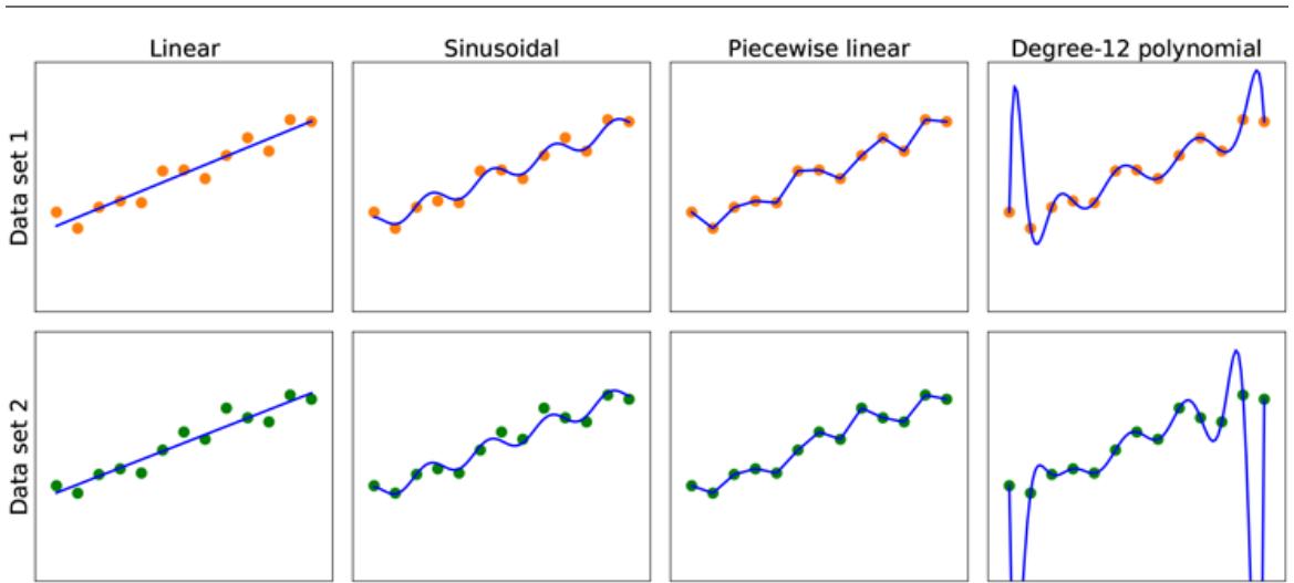
Figure 19.1

Finding hypotheses to fit data. Top row: four plots of best-fit functions from four different hypothesis spaces trained on data set 1. Bottom row: the same four functions, but trained on a slightly different data set (sampled from the same function).

One way to analyze hypothesis spaces is by the bias they impose (regardless of the training data set) and the variance they produce (from one training set to another).

Bias

By bias we mean (loosely) the tendency of a predictive hypothesis to deviate from the expected value when averaged over different training sets. Bias often results from restrictions imposed by the hypothesis space. For example, the hypothesis space of linear functions induces a strong bias: it only allows functions consisting of straight lines. If there are any patterns in the data other than the overall slope of a line, a linear function will not be able to represent those patterns. We say that a hypothesis is underfitting when it fails to find a pattern in the data. On the other hand, the piecewise linear function has low bias; the shape of the function is driven by the data.

Underfitting

By variance we mean the amount of change in the hypothesis due to fluctuation in the training data. The two rows of Figure 19.1 represent data sets that were each sampled from the same function. The data sets turned out to be slightly different. For the first three columns, the small difference in the data set translates into a small difference in the hypothesis. We call that low variance. But the degree-12 polynomials in the fourth column have high variance: look how different the two functions are at both ends of the -axis. Clearly, at least one of these polynomials must be a poor approximation to the true We say a function is overfitting the data when it pays too much attention to the particular data set it is trained on, causing it to perform poorly on unseen data.

Variance

Overfitting

Often there is a bias–variance tradeoff: a choice between more complex, low-bias hypotheses that fit the training data well and simpler, low-variance hypotheses that may generalize better. Albert Einstein said in 1933, “the supreme goal of all theory is to make the irreducible basic elements as simple and as few as possible without having to surrender the adequate representation of a single datum of experience.” In other words, Einstein recommends choosing the simplest hypothesis that matches the data. This principle can be traced further back to the 14th-century English philosopher William of Ockham. His principle that “plurality [of entities] should not be posited without necessity” is called Ockham’s razor because it is used to “shave off” dubious explanations. 2

2 The name is often misspelled as “Occam.”

Bias–variance tradeoff

Defining simplicity is not easy. It seems clear that a polynomial with only two parameters is simpler than one with thirteen parameters. We will make this intuition more precise in Section 19.3.4 . However, in Chapter 21 we will see that deep neural network models can often generalize quite well, even though they are very complex—some of them have billions of parameters. So the number of parameters by itself is not a good measure of a model’s fitness. Perhaps we should be aiming for “appropriateness,” not “simplicity” in a model class. We will consider this issue in Section 19.4.1 .

Which hypothesis is best in Figure 19.1 ? We can’t be certain. If we knew the data represented, say, the number of hits to a Web site that grows from day to day, but also cycles depending on the time of day, then we might favor the sinusoidal function. If we knew the data was definitely not cyclic but had high noise, that would favor the linear function.

In some cases, an analyst is willing to say not just that a hypothesis is possible or impossible, but rather how probable it is. Supervised learning can be done by choosing the hypothesis that is most probable given the data:

\[h^\* = \underset{h \in H}{\text{argmax}} \, P\left(h|data\right).\]

By Bayes’ rule this is equivalent to

\[h^\* = \underset{h \in H}{\text{argmax}} \, P(data \, \middle| \, h) \, P(h).\]

Then we can say that the prior probability is high for a smooth degree-1 or -2 polynomial and lower for a degree-12 polynomial with large, sharp spikes. We allow unusual-looking functions when the data say we really need them, but we discourage them by giving them a low prior probability.

Why not let be the class of all computer programs, or all Turing machines? The problem is that there is a tradeoff between the expressiveness of a hypothesis space and the computational complexity of finding a good hypothesis within that space. For example, fitting a straight line to data is an easy computation; fitting high-degree polynomials is somewhat harder; and fitting Turing machines is undecidable. A second reason to prefer simple hypothesis spaces is that presumably we will want to use after we have learned it, and computing when is a linear function is guaranteed to be fast, while computing an arbitrary Turing machine program is not even guaranteed to terminate.

For these reasons, most work on learning has focused on simple representations. In recent years there has been great interest in deep learning (Chapter 21 ), where representations are not simple but where the computation still takes only a bounded number of steps to compute with appropriate hardware.

We will see that the expressiveness–complexity tradeoff is not simple: it is often the case, as we saw with first-order logic in Chapter 8 , that an expressive language makes it possible for a simple hypothesis to fit the data, whereas restricting the expressiveness of the language means that any consistent hypothesis must be complex.

19.2.1 Example problem: Restaurant waiting

We will describe a sample supervised learning problem in detail: the problem of deciding whether to wait for a table at a restaurant. This problem will be used throughout the chapter to demonstrate different model classes. For this problem the output, is a Boolean variable that we will call WillWait; it is true for examples where we do wait for a table. The input, is a vector of ten attribute values, each of which has discrete values:

• 1. ALTERNATE: whether there is a suitable alternative restaurant nearby.
• 2. BAR: whether the restaurant has a comfortable bar area to wait in.
• 3. FRI/SAT: true on Fridays and Saturdays.
• 4. HUNGRY: whether we are hungry right now.
• 5. PATRONS: how many people are in the restaurant (values are None, Some, and Full).
• 6. PRICE: the restaurant’s price range
• 7. RAINING: whether it is raining outside.
• 8. RESERVATION: whether we made a reservation.
• 9. TYPE: the kind of restaurant (French, Italian, Thai, or burger).
• 10. WAITESTIMATE: host’s wait estimate:

A set of 12 examples, taken from the experience of one of us (SR), is shown in Figure 19.2 . Note how skimpy these data are: there are possible combinations of values for the input attributes, but we are given the correct output for only 12 of them; each of the other 9,204 could be either true or false; we don’t know. This is the essence of induction: we need to make our best guess at these missing 9,204 output values, given only the evidence of the 12 examples.

Figure 19.2

Example						Input Attributes					Output
	Alt	Bar	Fri	Hun	Pat	Price	Rain	Res	Type	Est	Will Wait
X1	Yes	No	No	Yes	Some	888	No	Yes	French	0-10	= Yes V1
X2	Yes	No	No	Yes	Full	S	No	No	Thai	30-60	= No V2
X3	No	Yes	No	No	Some	S	No	No	Burger	0-10	= Yes V3
X4	Yes	No	Yes	Yes	Full	S	Yes	No	Thai	10-30	Yes V4 ll
X5	Yes	No	Yes	No	Full	888	No	Yes	French	>60	= No V5
X6	No	Yes	No	Yes	Some	88	Yes	Yes	Italian	0-10	= Yes V6
X7	No	Yes	No	No	None	S	Yes	No	Burger	0-10	No V7 ==
X8	No	No	No	Yes	Some	88	Yes	Yes	Thai	0-10	= Yes V8
X9	No	Yes	Yes	No	Full	S	Yes	No	Burger	>60	= No V9
X10	Yes	Yes	Yes	Yes	Full	888	No	Yes	Italian	10-30	= No V10
X11	No	No	No	No	None	S	No	No	Thai	0-10	= No V11
X12	Yes	Yes	Yes	Yes	Full	S	No	No	Burger	30-60	Yes == V12

Examples for the restaurant domain.

19.3 Learning Decision Trees

A decision tree is a representation of a function that maps a vector of attribute values to a single output value—a “decision.” A decision tree reaches its decision by performing a sequence of tests, starting at the root and following the appropriate branch until a leaf is reached. Each internal node in the tree corresponds to a test of the value of one of the input attributes, the branches from the node are labeled with the possible values of the attribute, and the leaf nodes specify what value is to be returned by the function.

Decision tree

In general, the input and output values can be discrete or continuous, but for now we will consider only inputs consisting of discrete values and outputs that are either true (a positive example) or false (a negative example). We call this Boolean classification. We will use to index the examples ( is the input vector for the th example and is the output), and for the th attribute of the th example.

Positive

Negative

The tree representing the decision function that SR uses for the restaurant problem is shown in Figure 19.3 . Following the branches, we see that an example with and will be classified as positive (i.e., yes, we will wait for a table).

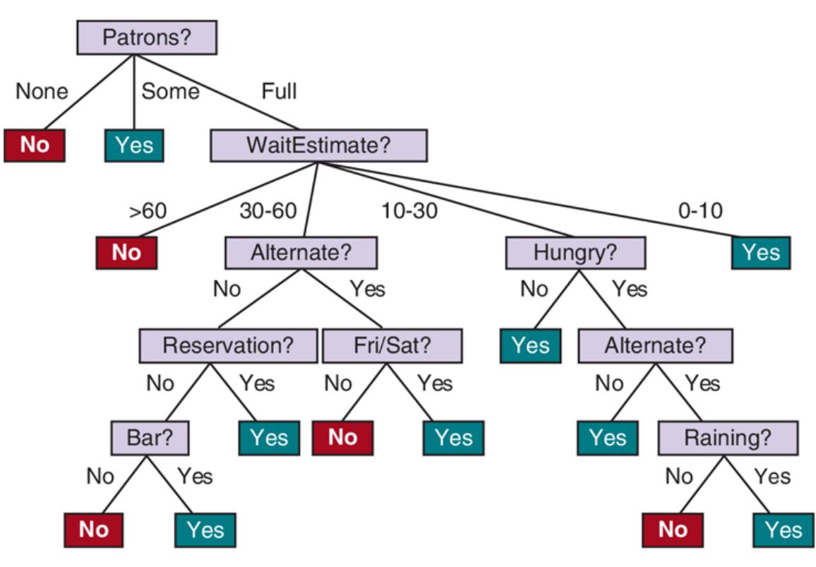
A decision tree for deciding whether to wait for a table.

19.3.1 Expressiveness of decision trees

A Boolean decision tree is equivalent to a logical statement of the form:

\[Output \iff \left(Path\_1 \lor Path\_2 \lor \cdots \right),\]

where each is a conjunction of the form of attribute-value tests corresponding to a path from the root to a true leaf. Thus, the whole expression is in disjunctive normal form, which means that any function in propositional logic can be expressed as a decision tree.

For many problems, the decision tree format yields a nice, concise, understandable result. Indeed, many “How To” manuals (e.g., for car repair) are written as decision trees. But some functions cannot be represented concisely. For example, the majority function, which returns true if and only if more than half of the inputs are true, requires an exponentially large decision tree, as does the parity function, which returns true if and only if an even number of input attributes are true. With real-valued attributes, the function is

hard to represent with a decision tree because the decision boundary is a diagonal line, and all decision tree tests divide the space up into rectangular, axis-aligned boxes. We would have to stack a lot of boxes to closely approximate the diagonal line. In other words, decision trees are good for some kinds of functions and bad for others.

Is there any kind of representation that is efficient for all kinds of functions? Unfortunately, the answer is no—there are just too many functions to be able to represent them all with a small number of bits. Even just considering Boolean functions with Boolean attributes, the truth table will have rows, and each row can output true or false, so there are different functions. With 20 attributes there are functions, so if we limit ourselves to a million-bit representation, we can’t represent all these functions.

19.3.2 Learning decision trees from examples

We want to find a tree that is consistent with the examples in Figure 19.2 and is as small as possible. Unfortunately, it is intractable to find a guaranteed smallest consistent tree. But with some simple heuristics, we can efficiently find one that is close to the smallest. The LEARN-DECISION-TREE algorithm adopts a greedy divide-and-conquer strategy: always test the most important attribute first, then recursively solve the smaller subproblems that are defined by the possible results of the test. By “most important attribute,” we mean the one that makes the most difference to the classification of an example. That way, we hope to get to the correct classification with a small number of tests, meaning that all paths in the tree will be short and the tree as a whole will be shallow.

Figure 19.4(a) shows that Type is a poor attribute, because it leaves us with four possible outcomes, each of which has the same number of positive as negative examples. On the other hand, in (b) we see that Patrons is a fairly important attribute, because if the value is None or Some, then we are left with example sets for which we can answer definitively (No and Yes, respectively). If the value is Full, we are left with a mixed set of examples. There are four cases to consider for these recursive subproblems:

• 1. If the remaining examples are all positive (or all negative), then we are done: we can answer Yes or No. Figure 19.4(b) shows examples of this happening in the None and Some branches.
• 2. If there are some positive and some negative examples, then choose the best attribute to split them. Figure 19.4(b) shows Hungry being used to split the

remaining examples.

• 3. If there are no examples left, it means that no example has been observed for this combination of attribute values, and we return the most common output value from the set of examples that were used in constructing the node’s parent.
• 4. If there are no attributes left, but both positive and negative examples, it means that these examples have exactly the same description, but different classifications. This can happen because there is an error or noise in the data; because the domain is nondeterministic; or because we can’t observe an attribute that would distinguish the examples. The best we can do is return the most common output value of the remaining examples.

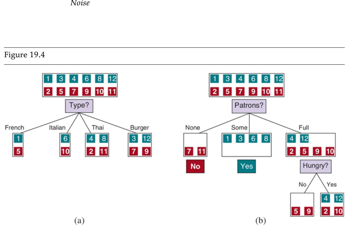
Splitting the examples by testing on attributes. At each node we show the positive (light boxes) and negative (dark boxes) examples remaining. (a) Splitting on Type brings us no nearer to distinguishing between positive and negative examples. (b) Splitting on Patrons does a good job of separating positive and negative examples. After splitting on Patrons, Hungry is a fairly good second test.

The LEARN-DECISION-TREE algorithm is shown in Figure 19.5 . Note that the set of examples is an input to the algorithm, but nowhere do the examples appear in the tree returned by the algorithm. A tree consists of tests on attributes in the interior nodes, values of attributes on

the branches, and output values on the leaf nodes. The details of the IMPORTANCE function are given in Section 19.3.3 . The output of the learning algorithm on our sample training set is shown in Figure 19.6 . The tree is clearly different from the original tree shown in Figure 19.3 . One might conclude that the learning algorithm is not doing a very good job of learning the correct function. This would be the wrong conclusion to draw, however. The learning algorithm looks at the examples, not at the correct function, and in fact, its hypothesis (see Figure 19.6 ) not only is consistent with all the examples, but is considerably simpler than the original tree! With slightly different examples the tree might be very different, but the function it represents would be similar.

Figure 19.5

The decision tree learning algorithm. The function IMPORTANCE is described in Section 19.3.3 . The function PLURALITY-VALUE selects the most common output value among a set of examples, breaking ties randomly.

Figure 19.6

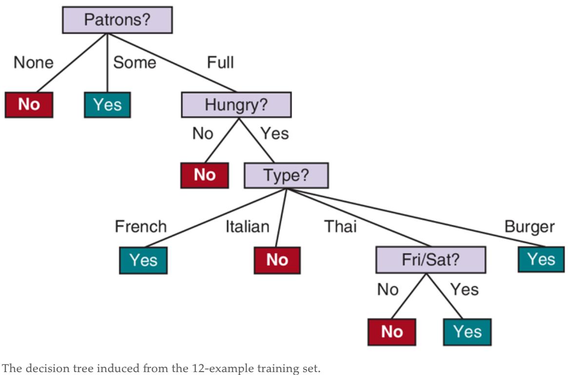
The learning algorithm has no reason to include tests for Raining and Reservation, because it can classify all the examples without them. It has also detected an interesting and previously unsuspected pattern: SR will wait for Thai food on weekends. It is also bound to make some mistakes for cases where it has seen no examples. For example, it has never seen a case where the wait is 0–10 minutes but the restaurant is full. In that case it says not to wait when Hungry is false, but SR would certainly wait. With more training examples the learning program could correct this mistake.

We can evaluate the performance of a learning algorithm with a learning curve, as shown in Figure 19.7 . For this figure we have 100 examples at our disposal, which we split randomly into a training set and a test set. We learn a hypothesis with the training set and measure its accuracy with the test set. We can do this starting with a training set of size 1 and increasing one at a time up to size 99. For each size, we actually repeat the process of randomly splitting into training and test sets 20 times, and average the results of the 20 trials. The curve shows that as the training set size grows, the accuracy increases. (For this reason, learning curves are also called happy graphs.) In this graph we reach 95% accuracy, and it looks as if the curve might continue to increase if we had more data.

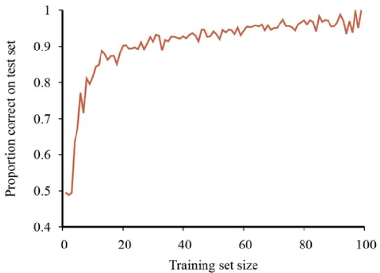
A learning curve for the decision tree learning algorithm on 100 randomly generated examples in the restaurant domain. Each data point is the average of 20 trials.

Learning curve

Happy graphs

19.3.3 Choosing attribute tests

The decision tree learning algorithm chooses the attribute with the highest IMPORTANCE. We will now show how to measure importance, using the notion of information gain, which is defined in terms of entropy, which is the fundamental quantity in information theory (Shannon and Weaver, 1949).

Entropy

Entropy is a measure of the uncertainty of a random variable; the more information, the less entropy. A random variable with only one possible value—a coin that always comes up heads—has no uncertainty and thus its entropy is defined as zero. A fair coin is equally likely to come up heads or tails when flipped, and we will soon show that this counts as “1 bit” of entropy. The roll of a fair four-sided die has 2 bits of entropy, because there are equally probable choices. Now consider an unfair coin that comes up heads 99% of the time. Intuitively, this coin has less uncertainty than the fair coin—if we guess heads we’ll be wrong only 1% of the time—so we would like it to have an entropy measure that is close to zero, but positive. In general, the entropy of a random variable with values having probability is defined as

\[\text{Entropy:} \quad H(V) = \sum\_{k} P(v\_k) \log\_2 \frac{1}{P(v\_k)} = -\sum\_{k} P(v\_k) \log\_2 P(v\_k).\]

We can check that the entropy of a fair coin flip is indeed 1 bit:

\[H(Fair) = -(0.5\log\_2 0.5 + 0.5\log\_2 0.5) = 1\]

And of a four-sided die is 2 bits:

\[H(Die4) = -(0.25\log\_2 0.25 + 0.25\log\_2 0.25 + 0.25\log\_2 0.25 + 0.25\log\_2 0.25) = 2.5\]

For the loaded coin with 99% heads, we get

\[H(Loaded) = -(0.99\log\_2 0.99 + 0.01\log\_2 0.01) \approx 0.08 \text{ bits}.\]

It will help to define as the entropy of a Boolean random variable that is true with probability

\[B(q) = -(q\log\_2 q + (1-q)\log\_2(1-q)).\]

Thus, Now let’s get back to decision tree learning. If a training set contains positive examples and negative examples, then the entropy of the output variable on the whole set is

\[H(Output) = B\left(\frac{p}{p+n}\right).\]

The restaurant training set in Figure 19.2 has so the corresponding entropy is or exactly 1 bit. The result of a test on an attribute will give us some information, thus reducing the overall entropy by some amount. We can measure this reduction by looking at the entropy remaining after the attribute test.

An attribute with distinct values divides the training set into subsets Each subset has positive examples and negative examples, so if we go along that branch, we will need an additional bits of information to answer the question. A randomly chosen example from the training set has the th value for the attribute (i.e., is in with probability ), so the expected entropy remaining after testing attribute is

\[Remainder(A) = \sum\_{k=1}^{d} \frac{p\_k + n\_k}{p + n} B\left(\frac{p\_k}{p\_k + n\_k}\right).\]

The information gain from the attribute test on is the expected reduction in entropy:

\[Gain(A) = B\left(\frac{p}{p+n}\right) - Remainder(A).\]

Information gain

In fact is just what we need to implement the IMPORTANCE function. Returning to the attributes considered in Figure 19.4 , we have

\[\begin{aligned} Gain(Patrons) &= 1 - \left[ \frac{2}{12} B\left(\frac{0}{2}\right) + \frac{4}{12} B\left(\frac{4}{4}\right) + \frac{6}{12} B\left(\frac{2}{6}\right) \right] \approx 0.541 \text{ bits}, \\ Gain(Type) &= 1 - \left[ \frac{2}{12} B\left(\frac{1}{2}\right) + \frac{2}{12} B\left(\frac{1}{2}\right) + \frac{4}{12} B\left(\frac{2}{4}\right) + \frac{4}{12} B\left(\frac{2}{4}\right) \right] = 0 \text{ bits}, \end{aligned}\]

confirming our intuition that Patrons is a better attribute to split on first. In fact, Patrons has the maximum information gain of any of the attributes and thus would be chosen by the decision tree learning algorithm as the root.

19.3.4 Generalization and overfitting

We want our learning algorithms to find a hypothesis that fits the training data, but more importantly, we want it to generalize well for previously unseen data. In Figure 19.1 we saw that a high-degree polynomial can fit all the data, but has wild swings that are not warranted by the data: it fits but can overfit. Overfitting becomes more likely as the number of attributes grows, and less likely as we increase the number of training examples. Larger hypothesis spaces (e.g., decision trees with more nodes or polynomials with high degree) have more capacity both to fit and to overfit; some model classes are more prone to overfitting than others.

For decision trees, a technique called decision tree pruning combats overfitting. Pruning works by eliminating nodes that are not clearly relevant. We start with a full tree, as generated by LEARN-DECISION-TREE. We then look at a test node that has only leaf nodes as descendants. If the test appears to be irrelevant—detecting only noise in the data—then we eliminate the test, replacing it with a leaf node. We repeat this process, considering each test with only leaf descendants, until each one has either been pruned or accepted as is.

Decision tree pruning

The question is, how do we detect that a node is testing an irrelevant attribute? Suppose we are at a node consisting of positive and negative examples. If the attribute is irrelevant, we would expect that it would split the examples into subsets such that each subset has roughly the same proportion of positive examples as the whole set, and so the information gain will be close to zero. Thus, a low information gain is a good clue that the attribute is irrelevant. Now the question is, how large a gain should we require in order to split on a particular attribute? 3

3 The gain will be strictly positive except for the unlikely case where all the proportions are exactly the same. (See Exercise 19.NNGA.)

We can answer this question by using a statistical significance test. Such a test begins by assuming that there is no underlying pattern (the so-called null hypothesis). Then the actual data are analyzed to calculate the extent to which they deviate from a perfect absence of pattern. If the degree of deviation is statistically unlikely (usually taken to mean a 5% probability or less), then that is considered to be good evidence for the presence of a

significant pattern in the data. The probabilities are calculated from standard distributions of the amount of deviation one would expect to see in random sampling.

Significance test

Null hypothesis

In this case, the null hypothesis is that the attribute is irrelevant and, hence, that the information gain for an infinitely large sample would be zero. We need to calculate the probability that, under the null hypothesis, a sample of size would exhibit the observed deviation from the expected distribution of positive and negative examples. We can measure the deviation by comparing the actual numbers of positive and negative examples in each subset, and with the expected numbers, and assuming true irrelevance:

\[ \hat{p}\_k = p \times \frac{p\_k + n\_k}{p + n} \qquad \qquad \hat{n}\_k = n \times \frac{p\_k + n\_k}{p + n}. \]

A convenient measure of the total deviation is given by

\[ \Delta = \sum\_{k=1}^{d} \frac{(p\_k - \hat{p}\_k)^2}{\hat{p}\_k} + \frac{(n\_k - \hat{n}\_k)^2}{\hat{n}\_k}. \]

Under the null hypothesis, the value of is distributed according to the (chi-squared) distribution with degrees of freedom. We can use a statistics function to see if a particular value confirms or rejects the null hypothesis. For example, consider the restaurant Type attribute, with four values and thus three degrees of freedom. A value of or more would reject the null hypothesis at the 5% level (and a value of or more would reject at the 1% level). Values below that lead to accepting the hypothesis that the attribute is irrelevant, and thus the associated branch of the tree should be pruned away. This is known as pruning.

pruning

With pruning, noise in the examples can be tolerated. Errors in the example’s label (e.g., an example that should be ) give a linear increase in prediction error, whereas errors in the descriptions of examples (e.g., when it was actually ) have an asymptotic effect that gets worse as the tree shrinks down to smaller sets. Pruned trees perform significantly better than unpruned trees when the data contain a large amount of noise. Also, the pruned trees are often much smaller and hence easier to understand and more efficient to execute.

One final warning: You might think that pruning and information gain look similar, so why not combine them using an approach called early stopping—have the decision tree algorithm stop generating nodes when there is no good attribute to split on, rather than going to all the trouble of generating nodes and then pruning them away. The problem with early stopping is that it stops us from recognizing situations where there is no one good attribute, but there are combinations of attributes that are informative. For example, consider the XOR function of two binary attributes. If there are roughly equal numbers of examples for all four combinations of input values, then neither attribute will be informative, yet the correct thing to do is to split on one of the attributes (it doesn’t matter which one), and then at the second level we will get splits that are very informative. Early stopping would miss this, but generate-and-then-prune handles it correctly.

Early stopping

19.3.5 Broadening the applicability of decision trees

Decision trees can be made more widely useful by handling the following complications:

MISSING DATA: In many domains, not all the attribute values will be known for every example. The values might have gone unrecorded, or they might be too expensive to obtain. This gives rise to two problems: First, given a complete decision tree, how

should one classify an example that is missing one of the test attributes? Second, how should one modify the information-gain formula when some examples have unknown values for the attribute? These questions are addressed in Exercise 19.MISS.

CONTINUOUS AND MULTIVALUED INPUT ATTRIBUTES: For continuous attributes like Height, Weight, or Time, it may be that every example has a different attribute value. The information gain measure would give its highest score to such an attribute, giving us a shallow tree with this attribute at the root, and single-example subtrees for each possible value below it. But that doesn’t help when we get a new example to classify with an attribute value that we haven’t seen before.

Split point

A better way to deal with continuous values is a split point test—an inequality test on the value of an attribute. For example, at a given node in the tree, it might be the case that testing on gives the most information. Efficient methods exist for finding good split points: start by sorting the values of the attribute, and then consider only split points that are between two examples in sorted order that have different classifications, while keeping track of the running totals of positive and negative examples on each side of the split point. Splitting is the most expensive part of realworld decision tree learning applications.

For attributes that are not continuous and do not have a meaningful ordering, but have a large number of possible values (e.g., Zipcode or CreditCardNumber), a measure called the information gain ratio (see Exercise 19.GAIN) can be used to avoid splitting into lots of single-example subtrees. Another useful approach is to allow an equality test of the form For example, the test could be used to pick out a large group of people in this zip code in New York City, and to lump everyone else into the “other” subtree.

CONTINUOUS-VALUED OUTPUT ATTRIBUTE: If we are trying to predict a numerical output value, such as the price of an apartment, then we need a regression tree rather than a classification tree. A regression tree has at each leaf a linear function of some subset of numerical attributes, rather than a single output value. For example, the branch for two-bedroom apartments might end with a linear function of square

footage and number of bathrooms. The learning algorithm must decide when to stop splitting and begin applying linear regression (see Section 19.6 ) over the attributes. The name CART, standing for Classification And Regression Trees, is used to cover both classes.

Regression tree

CART

A decision tree learning system for real-world applications must be able to handle all of these problems. Handling continuous-valued variables is especially important, because both physical and financial processes provide numerical data. Several commercial packages have been built that meet these criteria, and they have been used to develop thousands of fielded systems. In many areas of industry and commerce, decision trees are the first method tried when a classification method is to be extracted from a data set.

Decision trees have a lot going for them: ease of understanding, scalability to large data sets, and versatility in handling discrete and continuous inputs as well as classification and regression. However, they can have suboptimal accuracy (largely due to the greedy search), and if trees are very deep, then getting a prediction for a new example can be expensive in run time. Decision trees are also unstable in that adding just one new example can change the test at the root, which changes the entire tree. In Section 19.8.2 we will see that the random forest model can fix some of these issues.

Unstable

19.4 Model Selection and Optimization

Our goal in machine learning is to select a hypothesis that will optimally fit future examples. To make that precise we need to define “future example” and “optimal fit.”

First we will make the assumption that the future examples will be like the past. We call this the stationarity assumption; without it, all bets are off. We assume that each example has the same prior probability distribution:

\[\mathbf{P}\left(E\_{j}\right) = \mathbf{P}\left(E\_{j+1}\right) = \mathbf{P}\left(E\_{j+2}\right) = \cdots,\]

Stationarity

and is independent of the previous examples:

\[\mathbf{P}\left(E\_j\right) = \mathbf{P}\left(E\_j|E\_{j-1}, E\_{j-2}, \dots\right).\]

Examples that satisfy these equations are independent and identically distributed or i.i.d..

I.i.d.

The next step is to define “optimal fit.” For now, we will say that the optimal fit is the hypothesis that minimizes the error rate: the proportion of times that for an example. (Later we will expand on this to allow different errors to have different costs, in effect giving partial credit for answers that are “almost” correct.) We can estimate the error rate of a hypothesis by giving it a test: measure its performance on a test set of examples. It would be cheating for a hypothesis (or a student) to peek at the test answers before taking

the test. The simplest way to ensure this doesn’t happen is to split the examples you have into two sets: a training set to create the hypothesis, and a test set to evaluate it.

Error rate

If we are only going to create one hypothesis, then this approach is sufficient. But often we will end up creating multiple hypotheses: we might want to compare two completely different machine learning models, or we might want to adjust the various “knobs” within one model. For example, we could try different thresholds for pruning of decision trees, or different degrees for polynomials. We call these “knobs” hyperparameters—parameters of the model class, not of the individual model.

Hyperparameters

Suppose a researcher generates a hypotheses for one setting of the pruning hyperparameter, measures the error rates on the test set, and then tries different hyperparameters. No individual hypothesis has peeked at the test set data, but the overall process did, through the researcher.

The way to avoid this is to really hold out the test set—lock it away until you are completely done with training, experimenting, hyperparameter-tuning, re-training, etc. That means you need three data sets:

• 1. A training set to train candidate models.
• 2. A validation set, also known as a development set or dev set, to evaluate the candidate models and choose the best one.

Validation set

3. A test set to do a final unbiased evaluation of the best model.

What if we don’t have enough data to make all three of these data sets? We can squeeze more out of the data using a technique called -fold cross-validation. The idea is that each example serves double duty—as training data and validation data—but not at the same time. First we split the data into equal subsets. We then perform rounds of learning; on each round of the data are held out as a validation set and the remaining examples are used as the training set. The average test set score of the rounds should then be a better estimate than a single score. Popular values for are 5 and 10—enough to give an estimate that is statistically likely to be accurate, at a cost of 5 to 10 times longer computation time. The extreme is also known as leave-one-out cross-validation or LOOCV. Even with cross-validation, we still need a separate test set.

K-fold cross-validation

LOOCV

In Figure 19.1 (page 654) we saw a linear function underfit the data set, and a high-degree polynomial overfit the data. We can think of the task of finding a good hypothesis as two subtasks: model selection chooses a good hypothesis space, and optimization (also called training) finds the best hypothesis within that space. 4

⁴ Although the name “model selection” is in common use, a better name would have been “model class selection” or “hypothesis space selection.” The word “model” has been used in the literature to refer to three different levels of specificity: a broad hypothesis space (like “polynomials”), a hypothesis space with hyperparameters filled in (like “degree-2 polynomials”), and a specific hypothesis with all parameters filled in (like ).

Model selection

Optimization

Part of model selection is qualitative and subjective: we might select polynomials rather than decision trees based on something that we know about the problem. And part is quantitative and empirical: within the class of polynomials, we might select because that value performs best on the validation data set.

19.4.1 Model selection

Figure 19.8 describes a simple MODEL-SELECTION algorithm. It takes as argument a learning algorithm, Learner (for example, it could be LEARN-DECISION-TREE). Learner takes one hyperparameter, which is named size in the figure. For decision trees it could be the number of nodes in the tree; for polynomials size would be Degree. MODEL-SELECTION starts with the smallest value of size, yielding a simple model (which will probably underfit the data) and iterates through larger values of size, considering more complex models. In the end MODEL-SELECTION selects the model that has the lowest average error rate on the held-out validation data.

Figure 19.8

An algorithm to select the model that has the lowest validation error. It builds models of increasing complexity, and choosing the one with best empirical error rate, err, on the validation data set. Learner(size,examples) returns a hypothesis whose complexity is set by the parameter size, and which is trained on examples. In CROSS-VALIDATION, each iteration of the for loop selects a different slice of the examples as the validation set, and keeps the other examples as the training set. It then returns the average validation set error over all the folds. Once we have determined which value of the size parameter is best, MODEL-SELECTION returns the model (i.e., learner/hypothesis) of that size, trained on all the training examples, along with its error rate on the held-out test examples.

In Figure 19.9 we see two typical patterns that occur in model selection. In both (a) and (b) the training set error decreases monotonically (with slight random fluctuation) as we increase the complexity of the model. Complexity is measured by the number of decision tree nodes in (a) and by the number of neural network parameters in (b). For many model classes, the training set error reaches zero as the complexity increases.

Figure 19.9

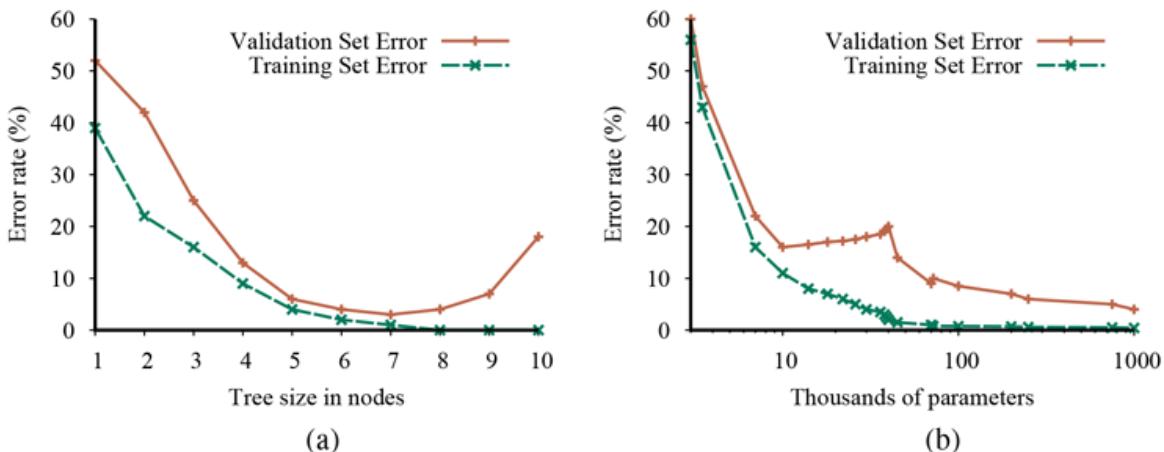
Error rates on training data (lower, green line) and validation data (upper, orange line) for models of different complexity on two different problems. MODEL-SELECTION picks the hyperparameter value with the lowest validation-set error. In (a) the model class is decision trees and the hyperparameter is the number of nodes. The data is from a version of the restaurant problem. The optimal size is 7. In (b) the model class is convolutional neural networks (see Section 21.3 ) and the hyperparameter is the number of regular parameters in the network. The data is the MNIST data set of images of digits; the task is to identify each digit. The optimal number of parameters is 1,000,000 (note the log scale).

The two cases differ markedly in validation set error. In (a) we see a U-shaped validationerror curve: error decreases for a while as model complexity increases, but then we reach a point where the model begins to overfit, and validation error rises. MODEL-SELECTION picks the value at the bottom of the U-shaped validation-error curve: in this case a tree with size 7. This is the spot that best balances underfitting and overfitting. In (b) we see an initial Ushaped curve just as in (a) but then the validation error starts to decrease again; the lowest validation error rate is the final point in the plot, with 1,000,000 parameters.

Why are some validation-error curves like (a) and some like (b)? It comes down to how the different model classes make use of excess capacity, and how well that matches up with the problem at hand. As we add capacity to a model class, we often reach the point where all the training examples can be represented perfectly within the model. For example, given a training set with distinct examples, there is always a decision tree with leaf nodes that can represent all the examples.

Interpolated

We say that a model that exactly fits all the training data has interpolated the data. Model classes typically start to overfit as the capacity approaches the point of interpolation. That seems to be because most of the model’s capacity is concentrated on the training examples, and the capacity that remains is allocated rather randomly in a way that is not representative of the patterns in the validation data set. Some model classes never recover from this overfitting, as with the decision trees in (a). But for other model classes, adding capacity means that there are more candidate functions, and some of them are naturally well-suited to the patterns of data that are in the true function The higher the capacity, the more of these suitable representations there are, and the more likely that the optimization mechanism will be able to land on one. 5

5 Some authors say the model has “memorized” the data.

Deep neural networks (Chapter 21 ), kernel machines (Section 19.7.5 ), random forests (Section 19.8.2 ), and boosted ensembles (Section 19.8.4 ) all have the property that their validation set error tends to decrease as capacity increases, as in Figure 19.9(b) .

We could extend the model selection algorithm in various ways: we could compare disparate model classes, by calling MODEL-SELECTION with DECISION-TREE-LEARNER as an argument and then with POLYNOMIAL-LEARNER, and seeing which does better. We could allow multiple hyperparameters, which means we would need a more complex optimization algorithm, such as a grid search (see Section 19.9.3 ) rather than a linear search.

19.4.2 From error rates to loss

So far, we have been trying to minimize error rate. This is clearly better than maximizing error rate, but it is not the full story. Consider the problem of classifying email messages as spam or non-spam. It is worse to classify non-spam as spam (and thus potentially miss an important message) than to classify spam as non-spam (and thus suffer a few seconds of annoyance). So a classifier with a 1% error rate, where almost all the errors were classifying spam as non-spam, would be better than a classifier with only a 0.5% error rate, if most of those errors were classifying non-spam as spam. We saw in Chapter 16 that decision makers should maximize expected utility, and utility is what learners should maximize as well. However, in machine learning it is traditional to express this as a negative: to minimize a loss function rather than maximize a utility function. The loss function

is defined as the amount of utility lost by predicting when the correct answer is

Loss function

This is the most general formulation of the loss function. Often a simplified version is used, that is independent of We will use the simplified version for the rest of this chapter, which means we can’t say that it is worse to misclassify a letter from Mom than it is to misclassify a letter from our annoying cousin, but we can say that it is 10 times worse to classify non-spam as spam than vice versa:

Note that is always zero; by definition there is no loss when you guess exactly right. For functions with discrete outputs, we can enumerate a loss value for each possible misclassification, but we can’t enumerate all the possibilities for real-valued data. If is 137.035999, we would be fairly happy with but just how happy should we be? In general, small errors are better than large ones; two functions that implement that idea are the absolute value of the difference (called the loss), and the square of the difference (called the loss; think “2” for square). For discrete-valued outputs, if we are content with the idea of minimizing error rate, we can use the loss function, which has a loss of 1 for an incorrect answer:

Theoretically, the learning agent maximizes its expected utility by choosing the hypothesis that minimizes expected loss over all input–output pairs it will see. To compute this expectation we need to define a prior probability distribution over examples. Let

be the set of all possible input–output examples. Then the expected generalization loss for a hypothesis (with respect to loss function ) is

\[GenLoss\_L(h) = \sum\_{(x,y)\in \varepsilon} L(y, h(x)) \, P(x, y) \,, .\]

Generalization loss

and the best hypothesis, is the one with the minimum expected generalization loss:

\[h^\* = \underset{h \in H}{\text{argmin}} \, GenLoss\_L(h).\]

Because is not known in most cases, the learning agent can only estimate generalization loss with empirical loss on a set of examples of size

\[EmpLoss\_{L,E}(h) = \sum\_{(x,y)\in E} L(y, h(x))\,\frac{1}{N} \,.\]

Empirical loss

The estimated best hypothesis is then the one with minimum empirical loss:

\[ \hat{h}^\* = \underset{h \in H}{\text{argmin }} EmpLoss\_{L,E}(h). \]

There are four reasons why may differ from the true function, unrealizability, variance, noise, and computational complexity.

First, we say that a learning problem is realizable if the hypothesis space actually contains the true function If is the set of linear functions, and the true function is a quadratic function, then no amount of data will recover the true Second, variance means that a

learning algorithm will in general return different hypotheses for different sets of examples. If the problem is realizable, then variance decreases towards zero as the number of training examples increases. Third, may be nondeterministic or noisy—it may return different values of for the same By definition, noise cannot be predicted (it can only be characterized). And finally, when is a complicated function in a large hypothesis space, it can be computationally intractable to systematically search all possibilities; in that case, a search can explore part of the space and return a reasonably good hypothesis, but can’t always guarantee the best one.

Realizable

Noise

Traditional methods in statistics and the early years of machine learning concentrated on small-scale learning, where the number of training examples ranged from dozens to the low thousands. Here the generalization loss mostly comes from the approximation error of not having the true in the hypothesis space, and from the estimation error of not having enough training examples to limit variance.

Small-scale learning

In recent years there has been more emphasis on large-scale learning, with millions of examples. Here the generalization loss may be dominated by limits of computation: there are enough data and a rich enough model that we could find an that is very close to the true but the computation to find it is complex, so we settle for an approximation.

Large-scale learning

19.4.3 Regularization

In Section 19.4.1 , we saw how to do model selection with cross-validation. An alternative approach is to search for a hypothesis that directly minimizes the weighted sum of empirical loss and the complexity of the hypothesis, which we will call the total cost:

Here is a hyperparameter, a positive number that serves as a conversion rate between loss and hypothesis complexity. If is chosen well, it nicely balances the empirical loss of a simple function against a complicated function’s tendency to overfit.

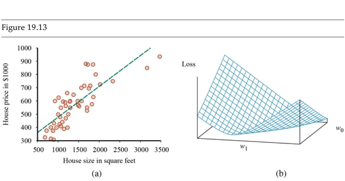
This process of explicitly penalizing complex hypotheses is called regularization: we’re looking for functions that are more regular. Note that we are now making two choices: the loss function ( or ), and the complexity measure, which is called a regularization function. The choice of regularization function depends on the hypothesis space. For example, for polynomials, a good regularization function is the sum of the squares of the coefficients—keeping the sum small would guide us away from the wiggly degree-12 polynomial in Figure 19.1 . We will show an example of this type of regularization in Section 19.6.3 .

Regularization

Regularization function

Another way to simplify models is to reduce the dimensions that the models work with. A process of feature selection can be performed to discard attributes that appear to be irrelevant. pruning is a kind of feature selection.

Feature selection

It is in fact possible to have the empirical loss and the complexity measured on the same scale, without the conversion factor they can both be measured in bits. First encode the hypothesis as a Turing machine program, and count the number of bits. Then count the number of bits required to encode the data, where a correctly predicted example costs zero bits and the cost of an incorrectly predicted example depends on how large the error is. The minimum description length or MDL hypothesis minimizes the total number of bits required. This works well in the limit, but for smaller problems the choice of encoding for the program—how best to encode a decision tree as a bit string—affects the outcome. In Chapter 20 (page 724), we describe a probabilistic interpretation of the MDL approach.

Minimum description length

19.4.4 Hyperparameter tuning

In Section 19.4.1 we showed how to select the best value of the hyperparameter size by applying cross-validation to each possible value until the validation error rate increases. That is a good approach when there is a single hyperparameter with a small number of possible values. But when there are multiple hyperparameters, or when they have continuous values, it is more difficult to choose good values.

The simplest approach to hyperparameter tuning is hand-tuning: guess some parameter values based on past experience, train a model, measure its performance on the validation data, analyze the results, and use your intuition to suggest new parameter values. Repeat

until you have satisfactory performance (or you run out of time, computing budget, or patience).

Hand-tuning

If there are only a few hyperparameters, each with a small number of possible values, then a more systematic approach called grid search is appropriate: try all combinations of values and see which performs best on the validation data. Different combinations can be run in parallel on different machines, so if you have sufficient computing resources, this need not be slow, although in some cases model selection has been known to suck up resources on thousand-computer clusters for days at a time.

Grid search

The search strategies from Chapters 3 and 4 can also come into play. For example, if two hyperparameters are independent of each other, they can be optimized separately.

If there are too many combinations of possible values, then random search samples uniformly from the set of all possible hyperparameter settings, repeating for as long as you are willing to spend the time and computational resources. Random sampling is also a good way to handle continuous values.

Random search

When each training run takes a long time, it can be helpful to get useful information out of each one. Bayesian optimization treats the task of choosing good hyperparameter values as a machine learning problem in itself. That is, think of the vector of hyperparameter values as an input, and the total loss on the validation set for the model built with those hyperparameters as an output, then we are trying to find the function that minimizes the loss Each time we do a training run we get a new pair, which we can use to update our belief about the shape of the function

Bayesian optimization

The idea is to trade off exploitation (choosing parameter values that are near to a previous good result) with exploration (trying novel parameter values). This is the same tradeoff we saw in Monte Carlo tree search (Section 5.4 ), and in fact the idea of upper confidence bounds is used here as well to minimize regret. If we make the assumption that can be approximated by a Gaussian process, then the math of updating our belief about works out nicely. Snoek et al. (2013) explain the math and give a practical guide to the approach, showing that it can outperform hand-tuning of parameters, even by experts.

Population-based training (PBT)

An alternative to Bayesian optimization is population-based training (PBT). PBT starts by using random search to train (in parallel) a population of models, each with different hyperparameter values. Then a second generation of models are trained, but they can choose hyperparameter values based on the successful values from the previous generation, as well as by random mutation, as in genetic algorithms (Section 4.1.4 ). Thus, populationbased training shares the advantage of random search that many runs can be done in parallel, and it shares the advantage of Bayesian optimization (or of hand-tuning by a clever human) that we can gain information from earlier runs to inform later ones.

19.5 The Theory of Learning

How can we be sure that our learned hypothesis will predict well for previously unseen inputs? That is, how do we know that the hypothesis is close to the target function if we don’t know what is? These questions have been pondered for centuries, by Ockham, Hume, and others. In recent decades, other questions have emerged: how many examples do we need to get a good What hypothesis space should we use? If the hypothesis space is very complex, can we even find the best or do we have to settle for a local maximum? How complex should be? How do we avoid overfitting? This section examines these questions.

We’ll start with the question of how many examples are needed for learning. We saw from the learning curve for decision tree learning on the restaurant problem (Figure 19.7 on page 661 ) that accuracy improves with more training data. Learning curves are useful, but they are specific to a particular learning algorithm on a particular problem. Are there some more general principles governing the number of examples needed?

Questions like this are addressed by computational learning theory, which lies at the intersection of AI, statistics, and theoretical computer science. The underlying principle is that any hypothesis that is seriously wrong will almost certainly be “found out” with high probability after a small number of examples, because it will make an incorrect prediction. Thus, any hypothesis that is consistent with a sufficiently large set of training examples is unlikely to be seriously wrong: that is, it must be probably approximately correct (PAC).

Computational learning theory

Probably approximately correct (PAC)

Any learning algorithm that returns hypotheses that are probably approximately correct is called a PAC learning algorithm; we can use this approach to provide bounds on the performance of various learning algorithms.

PAC learning

PAC-learning theorems, like all theorems, are logical consequences of axioms. When a theorem (as opposed to, say, a political pundit) states something about the future based on the past, the axioms have to provide the “juice” to make that connection. For PAC learning, the juice is provided by the stationarity assumption introduced on page 665 , which says that future examples are going to be drawn from the same fixed distribution as past examples. (Note that we do not have to know what distribution that is, just that it doesn’t change.) In addition, to keep things simple, we will assume that the true function is deterministic and is a member of the hypothesis space that is being considered.

The simplest PAC theorems deal with Boolean functions, for which the 0/1 loss is appropriate. The error rate of a hypothesis defined informally earlier, is defined formally here as the expected generalization error for examples drawn from the stationary distribution:

\[\text{error}(h) = \text{GenLoss}\_{L\_{0/1}}(h) = \sum\_{x,y} L\_{0/1}(y, h(x)) \, P(x, y).\]

In other words, is the probability that misclassifies a new example. This is the same quantity being measured experimentally by the learning curves shown earlier.

A hypothesis is called approximately correct if where is a small constant. We will show that we can find an such that, after training on examples, with high probability, all consistent hypotheses will be approximately correct. One can think of an approximately correct hypothesis as being “close” to the true function in hypothesis space: it lies inside what is called the around the true function The hypothesis space outside this ball is called

We can derive a bound on the probability that a “seriously wrong” hypothesis is consistent with the first examples as follows. We know that Thus, the probability that it agrees with a given example is at most Since the examples are independent, the bound for examples is:

\[P(h\_b \text{ agrees with } N \text{ examples}) \le (1 - \epsilon)^N.\]

The probability that contains at least one consistent hypothesis is bounded by the sum of the individual probabilities:

\[P(H\_{\text{bad}} \text{ contains a consistent hypothesis}) \le |H\_{\text{bad}}| (1 - \epsilon)^N \le |H| (1 - \epsilon)^N,\]

where we have used the fact that is a subset of and thus We would like to reduce the probability of this event below some small number

\[P(H\_{\text{bad}} \text{ contains a consistent hypothesis}) \le |H|(1 - \epsilon)^N \le \delta.\]

Given that we can achieve this if we allow the algorithm to see

(19.1)

\[N \geq \frac{1}{\epsilon} \left( \ln \frac{1}{\delta} + \ln |H| \right)\]

examples. Thus, with probability at least after seeing this many examples, the learning algorithm will return a hypothesis that has error at most In other words, it is probably approximately correct. The number of required examples, as a function of and is called the sample complexity of the learning algorithm.

Sample complexity

As we saw earlier, if is the set of all Boolean functions on attributes, then Thus, the sample complexity of the space grows as Because the number of possible examples is also this suggests that PAC-learning in the class of all Boolean functions requires seeing all, or nearly all, of the possible examples. A moment’s thought reveals the reason for this: contains enough hypotheses to classify any given set of examples in all possible ways. In particular, for any set of examples, the set of hypotheses consistent with those examples contains equal numbers of hypotheses that predict to be positive and hypotheses that predict to be negative.

To obtain real generalization to unseen examples, then, it seems we need to restrict the hypothesis space in some way; but of course, if we do restrict the space, we might eliminate the true function altogether. There are three ways to escape this dilemma.

The first is to bring prior knowledge to bear on the problem.

The second, which we introduced in Section 19.4.3 , is to insist that the algorithm return not just any consistent hypothesis, but preferably a simple one (as is done in decision tree learning). In cases where finding simple consistent hypotheses is tractable, the sample complexity results are generally better than for analyses based only on consistency.

The third, which we pursue next, is to focus on learnable subsets of the entire hypothesis space of Boolean functions. This approach relies on the assumption that the restricted hypothesis space contains a hypothesis that is close enough to the true function the benefits are that the restricted hypothesis space allows for effective generalization and is typically easier to search. We now examine one such restricted hypothesis space in more detail.

19.5.1 PAC learning example: Learning decision lists

We now show how to apply PAC learning to a new hypothesis space: decision lists. A decision list consists of a series of tests, each of which is a conjunction of literals. If a test succeeds when applied to an example description, the decision list specifies the value to be returned. If the test fails, processing continues with the next test in the list. Decision lists resemble decision trees, but their overall structure is simpler: they branch only in one direction. In contrast, the individual tests are more complex. Figure 19.10 shows a decision list that represents the following hypothesis:

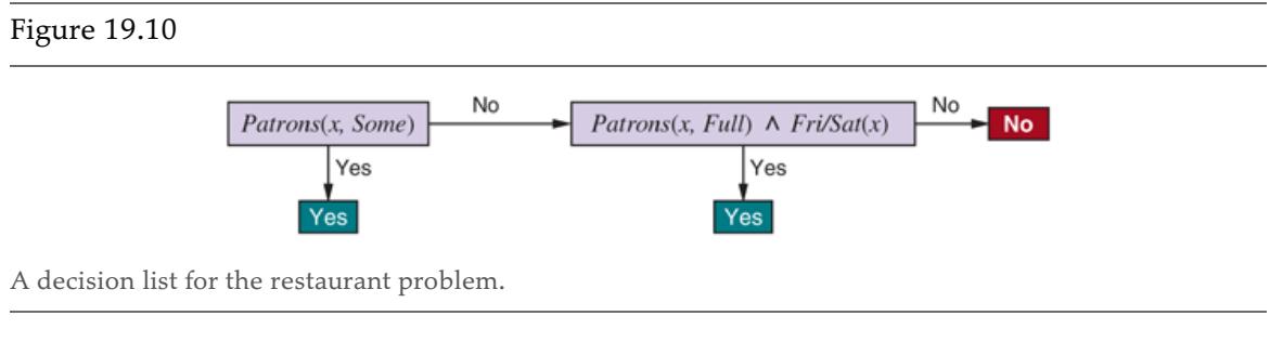
If we allow tests of arbitrary size, then decision lists can represent any Boolean function (Exercise 19.DLEX). On the other hand, if we restrict the size of each test to at most literals, then it is possible for the learning algorithm to generalize successfully from a small number of examples. We use the notation for a decision list with up to conjunctions. The example in Figure 19.10 is in 2-DL. It is easy to show (Exercise 19.DLEX) that includes as a subset the set of all decision trees of depth at most We will use the notation to denote a using Boolean attributes.

K-DT

The first task is to show that is learnable—that is, that any function in can be approximated accurately after training on a reasonable number of examples. To do this, we need to calculate the number of possible hypotheses. Let the set of conjunctions of at most literals using attributes be Because a decision list is constructed from tests, and because each test can be attached to either a Yes or a No outcome or can be absent from the decision list, there are at most distinct sets of component tests. Each of these sets of tests can be in any order, so

\[|k \text{-DL}(n)| \le 3^c c! \text{ where } c = |C \\ con j(n, k)|.\]

The number of conjunctions of at most literals from attributes is given by

\[\left| \operatorname{Con} j(n,k) \right| = \sum\_{i=0}^{k} \binom{2n}{i} = O(n^k).\]

Hence, after some work, we obtain

\[\left|k \operatorname{\cdotDL}(n)\right| = 2^{O(n^k \log\_2(n^k))}.\]

We can plug this into Equation (19.1) to show that the number of examples needed for PAC-learning a function is polynomial in

\[N \ge \frac{1}{\epsilon} \left( \ln \frac{1}{\delta} + O(n^k \log\_2(n^k)) \right).\]

Therefore, any algorithm that returns a consistent decision list will PAC-learn a function in a reasonable number of examples, for small

The next task is to find an efficient algorithm that returns a consistent decision list. We will use a greedy algorithm called DECISION-LIST-LEARNING that repeatedly finds a test that agrees exactly with some subset of the training set. Once it finds such a test, it adds it to the decision list under construction and removes the corresponding examples. It then constructs the remainder of the decision list, using just the remaining examples. This is repeated until there are no examples left. The algorithm is shown in Figure 19.11 .

Figure 19.11

An algorithm for learning decision lists.

This algorithm does not specify the method for selecting the next test to add to the decision list. Although the formal results given earlier do not depend on the selection method, it would seem reasonable to prefer small tests that match large sets of uniformly classified examples, so that the overall decision list will be as compact as possible. The simplest strategy is to find the smallest test that matches any uniformly classified subset, regardless of the size of the subset. Even this approach works quite well, as Figure 19.12 suggests. For this problem, the decision tree learns a bit faster than the decision list, but has more variation. Both methods are over 90% accurate after 100 trials.

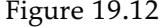
Learning curve for DECISION-LIST-LEARNING algorithm on the restaurant data. The curve for LEARN-DECISION-TREE is shown for comparison; decision trees do slightly better on this particular problem.

19.6 Linear Regression and Classification

Now it is time to move on from decision trees and lists to a different hypothesis space, one that has been used for hundreds of years: the class of linear functions of continuous-valued inputs. We’ll start with the simplest case: regression with a univariate linear function, otherwise known as “fitting a straight line.” Section 19.6.3 covers the multivariable case. Sections 19.6.4 and 19.6.5 show how to turn linear functions into classifiers by applying hard and soft thresholds.

Linear function

19.6.1 Univariate linear regression

A univariate linear function (a straight line) with input and output has the form where and are real-valued coefficients to be learned. We use the letter because we think of the coefficients as weights; the value of is changed by changing the relative weight of one term or another. We’ll define to be the vector and define the linear function with those weights as

\[h\_{\mathbf{w}}(x) = w\_1 x + w\_0.\]

Weight

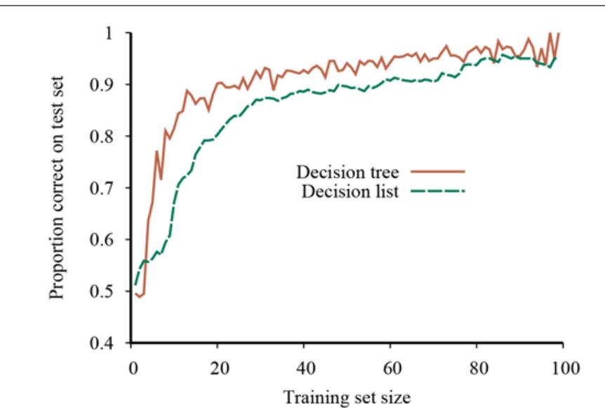
Figure 19.13(a) shows an example of a training set of points in the plane, each point representing the size in square feet and the price of a house offered for sale. The task of finding the that best fits these data is called linear regression. To fit a line to the data, all we have to do is find the values of the weights that minimize the empirical loss. It is traditional (going back to Gauss ) to use the squared-error loss function, summed over all the training examples: 6

6 Gauss showed that if the values have normally distributed noise, then the most likely values of and are obtained by using loss, minimizing the sum of the squares of the errors. (If the values have noise that follows a Laplace (double exponential) distribution, then loss is appropriate.)

\[Loss(h\_{\mathbf{w}}) = \sum\_{j=1}^{N} L\_2\left(y\_j, h\_{\mathbf{w}}\left(x\_j\right)\right) = \sum\_{j=1}^{N} \left(y\_j - h\_{\mathbf{w}}\left(x\_j\right)\right)^2 = \sum\_{j=1}^{N} \left(y\_j - \left(w\_1 x\_j + w\_0\right)\right)^2.\]

Linear regression

1. Data points of price versus floor space of houses for sale in Berkeley, CA, in July 2009, along with the linear function hypothesis that minimizes squared-error loss: (b) Plot of the loss function for various values of Note that the loss function is convex, with a single global minimum.

We would like to find The sum is minimized when its partial derivatives with respect to and are zero:

(19.2)

\[\frac{\partial}{\partial w\_0} \sum\_{j=1}^N (y\_j - (w\_1 x\_j + w\_0))^2 = 0 \text{ and } \frac{\partial}{\partial w\_1} \sum\_{j=1}^N (y\_j - (w\_1 x\_j + w\_0))^2 = 0.\]

These equations have a unique solution:

(19.3)

\[w\_1 = \frac{N\left(\sum x\_j y\_j\right) - \left(\sum x\_j\right)\left(\sum y\_j\right)}{N\left(\sum x\_j^2\right) - \left(\sum x\_j\right)^2}; \qquad w\_0 = \left(\sum y\_j - w\_1\left(\sum x\_j\right)\right) / N.\]

For the example in Figure 19.13(a) , the solution is and the line with those weights is shown as a dashed line in the figure.

Many forms of learning involve adjusting weights to minimize a loss, so it helps to have a mental picture of what’s going on in weight space—the space defined by all possible settings of the weights. For univariate linear regression, the weight space defined by and is two-dimensional, so we can graph the loss as a function of and in a 3D plot (see Figure 19.13(b) ). We see that the loss function is convex, as defined on page 122; this is true for every linear regression problem with an loss function, and implies that there are no local minima. In some sense that’s the end of the story for linear models; if we need to fit lines to data, we apply Equation (19.3) . 7

7 With some caveats: the loss function is appropriate when there is normally distributed noise that is independent of all results rely on the stationarity assumption; etc.

Weight space

19.6.2 Gradient descent

The univariate linear model has the nice property that it is easy to find an optimal solution where the partial derivatives are zero. But that won’t always be the case, so we introduce here a method for minimizing loss that does not depend on solving to find zeroes of the derivatives, and can be applied to any loss function, no matter how complex.

As discussed in Section 4.2 (page 119) we can search through a continuous weight space by incrementally modifying the parameters. There we called the algorithm hill climbing, but here we are minimizing loss, not maximizing gain, so we will use the term gradient descent. We choose any starting point in weight space—here, a point in the ( ) plane and then compute an estimate of the gradient and move a small amount in the steepest downhill direction, repeating until we converge on a point in weight space with (local) minimum loss. The algorithm is as follows:

(19.4)

Gradient descent

The parameter which we called the step size in Section 4.2 , is usually called the learning rate when we are trying to minimize loss in a learning problem. It can be a fixed constant, or it can decay over time as the learning process proceeds.

Learning rate

For univariate regression, the loss is quadratic, so the partial derivative will be linear. (The only calculus you need to know is the chain rule: plus the facts that and ) Let’s first work out the partial derivatives—the slopes—in the simplified case of only one training example,

(19.5)

\[\frac{\partial}{\partial w\_i} Loss(\mathbf{w}) \;= \; \frac{\partial}{\partial w\_i} (y - h\_{\mathbf{w}}(x))^2 \;= 2(y - h\_{\mathbf{w}}(x)) \times \frac{\partial}{\partial w\_i} (y - h\_{\mathbf{w}}(x))\]

\[= \; 2(y - h\_{\mathbf{w}}(x)) \times \frac{\partial}{\partial w\_i} (y - (w\_1 x + w\_0)).\]

Chain rule

Applying this to both and we get:

\[\frac{\partial}{\partial w\_0} Loss(\mathbf{w}) = -2 \left( y - h\_{\mathbf{w}}(x) \right); \qquad \frac{\partial}{\partial w\_1} Loss\left(\mathbf{w}\right) = -2 \left( y - h\_{\mathbf{w}}\left(x\right) \right) \times x.\]

Plugging this into Equation (19.4) , and folding the 2 into the unspecified learning rate we get the following learning rule for the weights:

\[w\_0 \gets w\_0 + \alpha \ (y - h\_{\mathbf{w}}(x)) \ ; \quad w\_1 \gets w\_1 + \alpha \ (y - h\_{\mathbf{w}}(x) \ ) \times \ x\]

These updates make intuitive sense: if (i.e., the output is too large), reduce a bit, and reduce if was a positive input but increase if was a negative input.

The preceding equations cover one training example. For training examples, we want to minimize the sum of the individual losses for each example. The derivative of a sum is the sum of the derivatives, so we have:

\[w\_0 \gets w\_0 + \alpha \sum\_j (y\_j - h\_{\mathbf{w}}(x\_j)) \; ; \quad w\_1 \gets w\_1 + \alpha \sum\_j (y\_j - h\_{\mathbf{w}}(x\_j)) \; \times \; x\_j \bar{x}\_j\]

These updates constitute the batch gradient descent learning rule for univariate linear regression (also called deterministic gradient descent). The loss surface is convex, which means that there are no local minima to get stuck in, and convergence to the global minimum is guaranteed (as long as we don’t pick an that is so large that it overshoots), but may be very slow: we have to sum over all training examples for every step, and there may be many steps. The problem is compounded if is larger than the processor’s memory size. A step that covers all the training examples is called an epoch.

Batch gradient descent

A faster variant is called stochastic gradient descent or SGD: it randomly selects a small number of training examples at each step, and updates according to Equation (19.5) . The original version of SGD selected only one training example for each step, but it is now more common to select a minibatch of out of the examples. Suppose we have examples and choose a minibatch of size Then on each step we have reduced the amount of computation by a factor of 100; but because the standard error of the estimated mean gradient is proportional to the square root of the number of examples, the standard error increases by only a factor of 10. So even if we have to take 10 times more steps before convergence, minibatch SGD is still 10 times faster than full batch SGD in this case.

Epoch

Stochastic gradient descent

SGD

Minibatch

With some CPU or GPU architectures, we can choose to take advantage of parallel vector operations, making a step with examples almost as fast as a step with only a single example. Within these constraints, we would treat as a hyperparameter that should be tuned for each learning problem.

Convergence of minibatch SGD is not strictly guaranteed; it can oscillate around the minimum without settling down. We will see on page 684 how a schedule of decreasing the learning rate, (as in simulated annealing) does guarantee convergence.

SGD can be helpful in an online setting, where new data are coming in one at a time, and the stationarity assumption may not hold. (In fact, SGD is also known as online gradient descent.) With a good choice for a model will slowly evolve, remembering some of what it learned in the past, but also adapting to the changes represented by the new data.

Online gradient descent

SGD is widely applied to models other than linear regression, in particular neural networks. Even when the loss surface is not convex, the approach has proven effective in finding good local minima that are close to the global minimum.

19.6.3 Multivariable linear regression

We can easily extend to multivariable linear regression problems, in which each example is an -element vector. Our hypothesis space is the set of functions of the form 8

8 The reader may wish to consult Appendix A for a brief summary of linear algebra. Also, note that we use the term “multivariable regression” to mean that the input is a vector of multiple values, but the output is a single variable. We will use the term “multivariate regression” for the case where the output is also a vector of multiple variables. However, other authors use the two terms interchangeably.

\[h\_{\mathbf{w}}(\mathbf{x}\_j) = w\_0 + w\_1 x\_{j,1} + \dots + w\_n x\_{j,n} = w\_0 + \sum\_i w\_i x\_{j,i} \dots\]

Multivariable linear regression

The term, the intercept, stands out as different from the others. We can fix that by inventing a dummy input attribute, which is defined as always equal to 1. Then is simply the dot product of the weights and the input vector (or equivalently, the matrix product of the transpose of the weights and the input vector):

\[h\_{\mathbf{w}}(\mathbf{x}\_j) = \mathbf{w} \cdot \mathbf{x}\_j = \mathbf{w}^\top \mathbf{x}\_j = \sum\_i w\_i x\_{j,i} \cdot \mathbf{x}\_i\]

The best vector of weights, minimizes squared-error loss over the examples:

\[\mathbf{w}^\* = \underset{\mathbf{w}}{\text{argmin}} \sum\_{j} L\_2(y\_j, \mathbf{w} \cdot \mathbf{x}\_j).\]

Multivariable linear regression is actually not much more complicated than the univariate case we just covered. Gradient descent will reach the (unique) minimum of the loss function; the update equation for each weight is

(19.6)

\[w\_i \gets w\_i + \alpha \sum\_j (y\_j - h\_{\mathbf{w}}(\mathbf{x}\_j)) \times x\_{j,i}\]

With the tools of linear algebra and vector calculus, it is also possible to solve analytically for the that minimizes loss. Let be the vector of outputs for the training examples, and be the data matrix—that is, the matrix of inputs with one -dimensional example per row. Then the vector of predicted outputs is and the squared-error loss over all the training data is

\[L(\mathbf{w}) = ||\hat{\mathbf{y}} - \mathbf{y}||^2 = ||\mathbf{X}\mathbf{w} - \mathbf{y}||^2.\]

Data matrix

We set the gradient to zero:

\[\nabla\_{\mathbf{w}} L(\mathbf{w}) = 2\mathbf{X}^{\top}(\mathbf{X}\mathbf{w} - \mathbf{y}) = 0.\]

Rearranging, we find that the minimum-loss weight vector is given by

\[\mathbf{w}^\* = (\mathbf{X}^\top \mathbf{X})^{-1} \mathbf{X}^\top \mathbf{y}.\]

We call the expression the pseudoinverse of the data matrix, and Equation (19.7) is called the normal equation.

Pseudoinverse

Normal equation

With univariate linear regression we didn’t have to worry about overfitting. But with multivariable linear regression in high-dimensional spaces it is possible that some dimension that is actually irrelevant appears by chance to be useful, resulting in overfitting.

Thus, it is common to use regularization on multivariable linear functions to avoid overfitting. Recall that with regularization we minimize the total cost of a hypothesis, counting both the empirical loss and the complexity of the hypothesis:

\[Cost(h) = EmpLoss(h) + \lambda\text{\textquotedbl{}Complexity(h)\textquotedbl{}}\]

For linear functions the complexity can be specified as a function of the weights. We can consider a family of regularization functions:

\[Complexity(h\_{\mathbf{w}}) = L\_q(\mathbf{w}) = \sum\_i |w\_i|^q.\]

As with loss functions, with we have regularization , which minimizes the sum of the absolute values; with regularization minimizes the sum of squares. Which regularization function should you pick? That depends on the specific problem, but regularization has an important advantage: it tends to produce a sparse model. That is, it often sets many weights to zero, effectively declaring the corresponding attributes to be 9

completely irrelevant—just as LEARN-DECISION-TREE does (although by a different mechanism). Hypotheses that discard attributes can be easier for a human to understand, and may be less likely to overfit.

9 It is perhaps confusing that the notation and is used for both loss functions and regularization functions. They need not be used in pairs: you could use loss with regularization, or vice versa.

Sparse model

Figure 19.14 gives an intuitive explanation of why regularization leads to weights of zero, while regularization does not. Note that minimizing is equivalent to minimizing subject to the constraint that for some constant that is related to Now, in Figure 19.14(a) the diamond-shaped box represents the set of points in two-dimensional weight space that have complexity less than our solution will have to be somewhere inside this box. The concentric ovals represent contours of the loss function, with the minimum loss at the center. We want to find the point in the box that is closest to the minimum; you can see from the diagram that, for an arbitrary position of the minimum and its contours, it will be common for the corner of the box to find its way closest to the minimum, just because the corners are pointy. And of course the corners are the points that have a value of zero in some dimension.

Figure 19.14

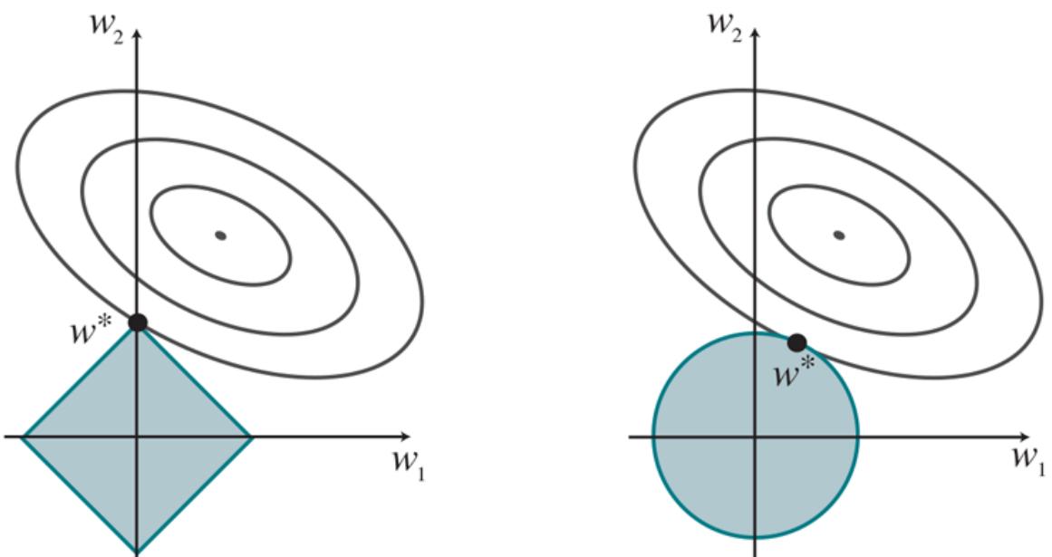
Why regularization tends to produce a sparse model. Left: With regularization (box), the minimal achievable loss (concentric contours) often occurs on an axis, meaning a weight of zero. Right: With regularization (circle), the minimal loss is likely to occur anywhere on the circle, giving no preference to zero weights.

In Figure 19.14(b) , we’ve done the same for the complexity measure, which represents a circle rather than a diamond. Here you can see that, in general, there is no reason for the intersection to appear on one of the axes; thus regularization does not tend to produce zero weights. The result is that the number of examples required to find a good is linear in the number of irrelevant features for regularization, but only logarithmic with regularization. Empirical evidence on many problems supports this analysis.

Another way to look at it is that regularization takes the dimensional axes seriously, while treats them as arbitrary. The function is spherical, which makes it rotationally invariant: Imagine a set of points in a plane, measured by their and coordinates. Now imagine rotating the axes by You’d get a different set of values representing the same points. If you apply regularization before and after rotating, you get exactly the same point as the answer (although the point would be described with the new coordinates). That is appropriate when the choice of axes really is arbitrary—when it doesn’t matter whether your two dimensions are distances north and east; or distances northeast and southeast. With regularization you’d get a different answer, because the function is not rotationally invariant. That is appropriate when the axes are not interchangeable; it doesn’t make sense to rotate “number of bathrooms” towards “lot size.”

19.6.4 Linear classifiers with a hard threshold

Linear functions can be used to do classification as well as regression. For example, Figure 19.15(a) shows data points of two classes: earthquakes (which are of interest to seismologists) and underground explosions (which are of interest to arms control experts). Each point is defined by two input values, and that refer to body and surface wave magnitudes computed from the seismic signal. Given these training data, the task of classification is to learn a hypothesis that will take new points and return either 0 for earthquakes or 1 for explosions.

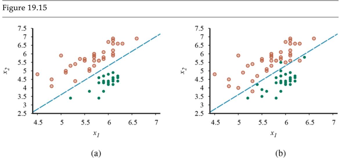
1. Plot of two seismic data parameters, body wave magnitude and surface wave magnitude for earthquakes (open orange circles) and nuclear explosions (green circles) occurring between 1982 and 1990 in Asia and the Middle East (Kebeasy et al., 1998). Also shown is a decision boundary between the classes. (b) The same domain with more data points. The earthquakes and explosions are no longer linearly separable.

A decision boundary is a line (or a surface, in higher dimensions) that separates the two classes. In Figure 19.15(a) , the decision boundary is a straight line. A linear decision boundary is called a linear separator and data that admit such a separator are called linearly separable. The linear separator in this case is defined by

\[x\_2 = 1.7x\_1 - 4.9 \quad \text{or} \quad -4.9 + 1.7x\_1 - x\_2 = 0.\]

Decision boundary

Linear separator

Linear separability

The explosions, which we want to classify with value 1, are below and to the right of this line; they are points for which while earthquakes have We can make the equation easier to deal with by changing it into the vector dot product form—with we have

\[-4.9x\_0 + 1.7x\_1 - x\_2 = 0,\]

and we can define the vector of weights,

\[ \mathbf{w} = \langle -4.9, 1.7, -1 \rangle, \]

and write the classification hypothesis

\[h\_{\mathbf{w}}(\mathbf{x}) = 1 \text{ if } \mathbf{w} \cdot \mathbf{x} \ge 0 \text{ and } 0 \text{ otherwise.}\]

Alternatively, we can think of as the result of passing the linear function through a threshold function:

Threshold function

The threshold function is shown in Figure 19.17(a) .

Now that the hypothesis has a well-defined mathematical form, we can think about choosing the weights to minimize the loss. In Sections 19.6.1 and 19.6.3 , we did this both in closed form (by setting the gradient to zero and solving for the weights) and by gradient descent in weight space. Here we cannot do either of those things because the gradient is zero almost everywhere in weight space except at those points where and at those points the gradient is undefined.

There is, however, a simple weight update rule that converges to a solution—that is, to a linear separator that classifies the data perfectly—provided the data are linearly separable. For a single example we have

(19.8)

\[w\_i \gets w\_i + \alpha \left( y - h\_{\mathbf{w}}(\mathbf{x}) \right) \times x\_i\]

which is essentially identical to Equation (19.6) , the update rule for linear regression! This rule is called the perceptron learning rule, for reasons that will become clear in Chapter 21 . Because we are considering a 0/1 classification problem, however, the behavior is somewhat different. Both the true value and the hypothesis output are either 0 or 1, so there are three possibilities:

• If the output is correct (i.e., ) then the weights are not changed.
• If is 1 but is 0, then is increased when the corresponding input is positive and decreased when is negative. This makes sense, because we want to make bigger so that outputs a 1.
• If is 0 but is 1, then is decreased when the corresponding input is positive and increased when is negative. This makes sense, because we want to make smaller so that outputs a 0.

Perceptron learning rule

Typically the learning rule is applied one example at a time, choosing examples at random (as in stochastic gradient descent). Figure 19.16(a) shows a training curve for this learning rule applied to the earthquake/explosion data shown in Figure 19.15(a) . A training curve measures the classifier performance on a fixed training set as the learning process proceeds one update at a time on that training set. The curve shows the update rule converging to a zero-error linear separator. The “convergence” process isn’t exactly pretty, but it always works. This particular run takes 657 steps to converge, for a data set with 63 examples, so each example is presented roughly 10 times on average. Typically, the variation across runs is large.

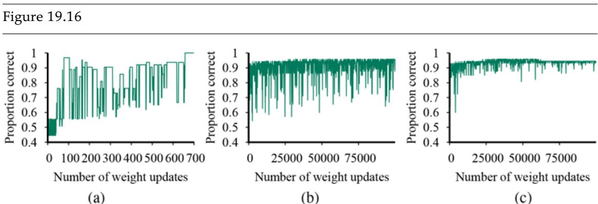
1. Plot of total training-set accuracy vs. number of iterations through the training set for the perceptron learning rule, given the earthquake/explosion data in Figure 19.15(a) . (b) The same plot for the noisy, nonseparable data in Figure 19.15(b) ; note the change in scale of the -axis. (c) The same plot as in (b), with a learning rate schedule

Training curve

We have said that the perceptron learning rule converges to a perfect linear separator when the data points are linearly separable; but what if they are not? This situation is all too common in the real world. For example, Figure 19.15(b) adds back in the data points left out by Kebeasy et al., (1998) when they plotted the data shown in Figure 19.15(a) . In Figure 19.16(b) , we show the perceptron learning rule failing to converge even after 10,000 steps: even though it hits the minimum-error solution (three errors) many times, the algorithm keeps changing the weights. In general, the perceptron rule may not converge to a stable solution for fixed learning rate but if decays as where is the iteration number, then the rule can be shown to converge to a minimum-error solution when examples are presented in a random sequence. It can also be shown that finding the 10

minimum-error solution is NP-hard, so one expects that many presentations of the examples will be required for convergence to be achieved. Figure 19.16(c) shows the training process with a learning rate schedule convergence is not perfect after 100,000 iterations, but it is much better than the fixed- case.

10 Technically, we require that and The learning rate satisfies these conditions. Often we use for some fairly large constant

19.6.5 Linear classification with logistic regression

We have seen that passing the output of a linear function through the threshold function creates a linear classifier; yet the hard nature of the threshold causes some problems: the hypothesis is not differentiable and is in fact a discontinuous function of its inputs and its weights. This makes learning with the perceptron rule a very unpredictable adventure. Furthermore, the linear classifier always announces a completely confident prediction of 1 or 0, even for examples that are very close to the boundary; it would be better if it could classify some examples as a clear 0 or 1, and others as unclear borderline cases.

All of these issues can be resolved to a large extent by softening the threshold function approximating the hard threshold with a continuous, differentiable function. In Chapter 13 (page 424), we saw two functions that look like soft thresholds: the integral of the standard normal distribution (used for the probit model) and the logistic function (used for the logit model). Although the two functions are very similar in shape, the logistic function

\[Logistic(z) = \frac{1}{1 + e^{-z}}\]

has more convenient mathematical properties. The function is shown in Figure 19.17(b) . With the logistic function replacing the threshold function, we now have

\[h\_{\mathbf{w}}(\mathbf{x}) = \operatorname{Logistic}(\mathbf{w} \cdot \mathbf{x}) = \frac{1}{1 + e^{-\mathbf{w} \cdot \mathbf{x}}}.\]

Figure 19.17

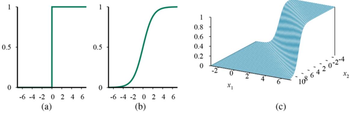
1. The hard threshold function with 0/1 output. Note that the function is nondifferentiable at (b) The logistic function, also known as the sigmoid function. (c) Plot of a logistic regression hypothesis for the data shown in Figure 19.15(b) .

An example of such a hypothesis for the two-input earthquake/explosion problem is shown in Figure 19.17(c) . Notice that the output, being a number between 0 and 1, can be interpreted as a probability of belonging to the class labeled 1. The hypothesis forms a soft boundary in the input space and gives a probability of 0.5 for any input at the center of the boundary region, and approaches 0 or 1 as we move away from the boundary.

The process of fitting the weights of this model to minimize loss on a data set is called logistic regression. There is no easy closed-form solution to find the optimal value of with this model, but the gradient descent computation is straightforward. Because our hypotheses no longer output just 0 or 1, we will use the loss function; also, to keep the formulas readable, we’ll use to stand for the logistic function, with its derivative.

Logistic regression

For a single example the derivation of the gradient is the same as for linear regression (Equation (19.5) ) up to the point where the actual form of is inserted. (For this derivation, we again need the chain rule.) We have

\[\begin{split} \frac{\partial}{\partial w\_i} Loss(\mathbf{w}) &= \frac{\partial}{\partial w\_i} (y - h\_{\mathbf{w}}(\mathbf{x}))^2 \\ &= 2(y - h\_{\mathbf{w}}(\mathbf{x})) \times \frac{\partial}{\partial w\_i} (y - h\_{\mathbf{w}}(\mathbf{x})) \\ &= -2(y - h\_{\mathbf{w}}(\mathbf{x})) \times g'(\mathbf{w} \cdot \mathbf{x}) \times \frac{\partial}{\partial w\_i} \mathbf{w} \cdot \mathbf{x} \\ &= -2(y - h\_{\mathbf{w}}(\mathbf{x})) \times g'(\mathbf{w} \cdot \mathbf{x}) \times x\_i. \end{split}\]

The derivative of the logistic function satisfies so we have

\[g'(\mathbf{w} \cdot \mathbf{x}) = g(\mathbf{w} \cdot \mathbf{x})(1 - g(\mathbf{w} \cdot \mathbf{x})) = h\_{\mathbf{w}}(\mathbf{x})(1 - h\_{\mathbf{w}}(\mathbf{x})) \]

so the weight update for minimizing the loss takes a step in the direction of the difference between input and prediction, and the length of that step depends on the constant and

(19.9)

\[w\_i \gets w\_i + \alpha \left( y - h\_{\mathbf{w}}(\mathbf{x}) \right) \times h\_{\mathbf{w}}(\mathbf{x}) (1 - h\_{\mathbf{w}}(\mathbf{x})) \times x\_i\]

Repeating the experiments of Figure 19.16 with logistic regression instead of the linear threshold classifier, we obtain the results shown in Figure 19.18 . In (a), the linearly separable case, logistic regression is somewhat slower to converge, but behaves much more predictably. In (b) and (c), where the data are noisy and nonseparable, logistic regression converges far more quickly and reliably. These advantages tend to carry over into real-world applications, and logistic regression has become one of the most popular classification techniques for problems in medicine, marketing, survey analysis, credit scoring, public health, and other applications.

Figure 19.18

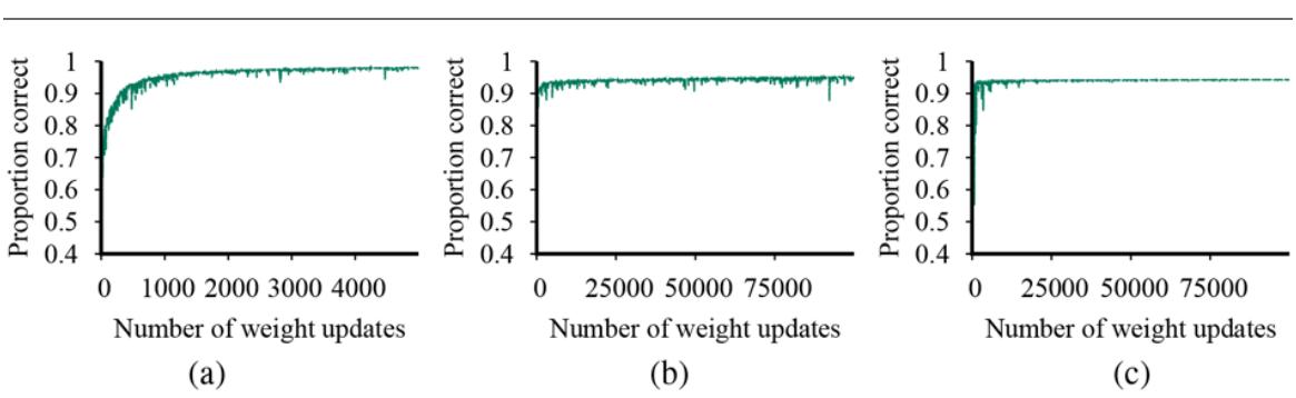
Repeat of the experiments in Figure 19.16 using logistic regression. The plot in (a) covers 5000 iterations rather than 700, while the plots in (b) and (c) use the same scale as before.

19.7 Nonparametric Models

Linear regression uses the training data to estimate a fixed set of parameters That defines our hypothesis and at that point we can throw away the training data, because they are all summarized by A learning model that summarizes data with a set of parameters of fixed size (independent of the number of training examples) is called a parametric model.

Parametric model

When data sets are small, it makes sense to have a strong restriction on the allowable hypotheses, to avoid overfitting. But when there are millions or billions of examples to learn from, it seems like a better idea to let the data speak for themselves rather than forcing them to speak through a tiny vector of parameters. If the data say that the correct answer is a very wiggly function, we shouldn’t restrict ourselves to linear or slightly wiggly functions.

Nonparametric model

Instance-based learning

A nonparametric model is one that cannot be characterized by a bounded set of parameters. For example, the piecewise linear function from Figure 19.1 retains all the data points as part of the model. Learning methods that do this have also been described as instance-based learning or memory-based learning. The simplest instance-based learning method is table lookup: take all the training examples, put them in a lookup table, and then when asked for see if is in the table; if it is, return the corresponding

The problem with this method is that it does not generalize well: when is not in the table we have no information about a plausible value.

19.7.1 Nearest-neighbor models

We can improve on table lookup with a slight variation: given a query instead of finding an example that is equal to find the examples that are nearest to This is called nearest-neighbors lookup. We’ll use the notation to denote the set of neighbors nearest to

Nearest neighbors

To do classification, find the set of neighbors and take the most common output value—for example, if and the output values are then the classification will be Yes. To avoid ties on binary classification, is usually chosen to be an odd number.

To do regression, we can take the mean or median of the neighbors, or we can solve a linear regression problem on the neighbors. The piecewise linear function from Figure 19.1 solves a (trivial) linear regression problem with the two data points to the right and left of (When the data points are equally spaced, these will be the two nearest neighbors.)

In Figure 19.19 , we show the decision boundary of -nearest-neighbors classification for 1 and 5 on the earthquake data set from Figure 19.15 . Nonparametric methods are still subject to underfitting and overfitting, just like parametric methods. In this case 1-nearestneighbors is overfitting; it reacts too much to the black outlier in the upper right and the white outlier at (5.4, 3.7). The 5-nearest-neighbors decision boundary is good; higher would underfit. As usual, cross-validation can be used to select the best value of

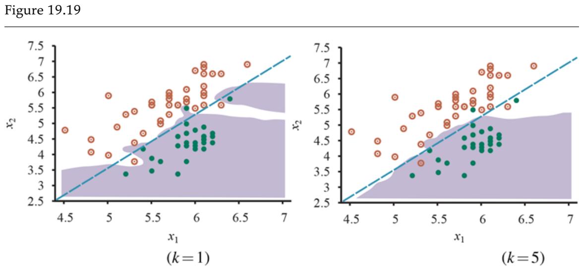
1. A -nearest-neighbors model showing the extent of the explosion class for the data in Figure 19.15 , with Overfitting is apparent. (b) With the overfitting problem goes away for this data set.

The very word “nearest” implies a distance metric. How do we measure the distance from a query point to an example point Typically, distances are measured with a Minkowski distance or norm, defined as

\[L^p(\mathbf{x}\_j, \mathbf{x}\_q) = \left(\sum\_i \left| x\_{j,i} - x\_{q,i} \right|^p \right)^{1/p}\]

Minkowski distance

With this is Euclidean distance and with it is Manhattan distance. With Boolean attribute values, the number of attributes on which the two points differ is called the Hamming distance. Often Euclidean distance is used if the dimensions are measuring similar properties, such as the width, height and depth of parts, and Manhattan distance is used if they are dissimilar, such as age, weight, and gender of a patient. Note that if we use the raw numbers from each dimension then the total distance will be affected by a change in units in any dimension. That is, if we change the height dimension from meters to miles while keeping the width and depth dimensions the same, we’ll get different nearest neighbors. And how do we compare a difference in age to a difference in weight? A

common approach is to applynormalization to the measurements in each dimension. We can compute the mean and standard deviation of the values in each dimension, and rescale them so that becomes A more complex metric known as the Mahalanobis distance takes into account the covariance between dimensions.

Hamming distance

Normalization

Mahalanobis distances

In low-dimensional spaces with plenty of data, nearest neighbors works very well: we are likely to have enough nearby data points to get a good answer. But as the number of dimensions rises we encounter a problem: the nearest neighbors in high-dimensional spaces are usually not very near! Consider -nearest-neighbors on a data set of points uniformly distributed throughout the interior of an -dimensional unit hypercube. We’ll define the neighborhood of a point as the smallest hypercube that contains the nearest neighbors. Let be the average side length of a neighborhood. Then the volume of the neighborhood (which contains points) is and the volume of the full cube (which contains points) is 1. So, on average, Taking th roots of both sides we get

To be concrete, let and In two dimensions ( a unit square), the average neighborhood has a small fraction of the unit square, and in 3 dimensions is just 2% of the edge length of the unit cube. But by the time we get to 17 dimensions, is half the edge length of the unit hypercube, and in 200 dimensions it is 94%. This problem has been called the curse of dimensionality.

Curse of dimensionality

Another way to look at it: consider the points that fall within a thin shell making up the outer 1% of the unit hypercube. These are outliers; in general it will be hard to find a good value for them because we will be extrapolating rather than interpolating. In one dimension, these outliers are only 2% of the points on the unit line (those points where or ), but in 200 dimensions, over 98% of the points fall within this thin shell—almost all the points are outliers. You can see an example of a poor nearest-neighbors fit on outliers if you look ahead to Figure 19.20(b) .

The function is conceptually trivial: given a set of examples and a query iterate through the examples, measure the distance to from each one, and keep the best If we are satisfied with an implementation that takes execution time, then that is the end of the story. But instance-based methods are designed for large data sets, so we would like something faster. The next two subsections show how trees and hash tables can be used to speed up the computation.

19.7.2 Finding nearest neighbors with -d trees

A balanced binary tree over data with an arbitrary number of dimensions is called a k-d tree, for -dimensional tree. The construction of a -d tree is similar to the construction of a balanced binary tree. We start with a set of examples and at the root node we split them along the th dimension by testing whether where is the median of the examples along the th dimension; thus half the examples will be in the left branch of the tree and half in the right. We then recursively make a tree for the left and right sets of examples, stopping when there are fewer than two examples left. To choose a dimension to split on at each node of the tree, one can simply select dimension at level of the tree. (Note that we may need to split on any given dimension several times as we proceed down the tree.) Another strategy is to split on the dimension that has the widest spread of values.

K-d tree

Exact lookup from a -d tree is just like lookup from a binary tree (with the slight complication that you need to pay attention to which dimension you are testing at each node). But nearest-neighbor lookup is more complicated. As we go down the branches, splitting the examples in half, in some cases we can ignore half of the examples. But not always. Sometimes the point we are querying for falls very close to the dividing boundary. The query point itself might be on the left hand side of the boundary, but one or more of the nearest neighbors might actually be on the right-hand side.

We have to test for this possibility by computing the distance of the query point to the dividing boundary, and then searching both sides if we can’t find examples on the left that are closer than this distance. Because of this problem, -d trees are appropriate only when there are many more examples than dimensions, preferably at least examples. Thus, -d trees are a good choice for up to about 10 dimensions when there are thousands of examples or up to 20 dimensions with millions of examples.

19.7.3 Locality-sensitive hashing

Hash tables have the potential to provide even faster lookup than binary trees. But how can we find nearest neighbors using a hash table, when hash codes rely on an exact match? Hash codes randomly distribute values among the bins, but we want to have near points grouped together in the same bin; we want a locality-sensitive hash (LSH).

Locality-sensitive hash

Approximate near-neighbors

We can’t use hashes to solve exactly, but with a clever use of randomized algorithms, we can find an approximate solution. First we define the approximate nearneighbors problem: given a data set of example points and a query point find, with high probability, an example point (or points) that is near To be more precise, we require that if there is a point that is within a radius of then with high probability the algorithm

will find a point that is within distance of If there is no point within radius then the algorithm is allowed to report failure. The values of and “high probability” are hyperparameters of the algorithm.

To solve approximate near neighbors, we will need a hash function that has the property that, for any two points and the probability that they have the same hash code is small if their distance is more than and is high if their distance is less than For simplicity we will treat each point as a bit string. (Any features that are not Boolean can be encoded into a set of Boolean features.)

We rely on the intuition that if two points are close together in an -dimensional space, then they will necessarily be close when projected down onto a one-dimensional space (a line). In fact, we can discretize the line into bins—hash buckets—so that, with high probability, near points project down to the same bin. Points that are far away from each other will tend to project down into different bins, but there will always be a few projections that coincidentally project far-apart points into the same bin. Thus, the bin for point contains many (but not all) points that are near and it might contain some points that are far away.

The trick of LSH is to create multiple random projections and combine them. A random projection is just a random subset of the bit-string representation. We choose different random projections and create hash tables, We then enter all the examples into each hash table. Then when given a query point we fetch the set of points in bin of each hash table, and union these sets together into a set of candidate points, Then we compute the actual distance to for each of the points in and return the closest points. With high probability, each of the points that are near to will show up in at least one of the bins, and although some far-away points will show up as well, we can ignore those. With large real-world problems, such as finding the near neighbors in a data set of 13 million Web images using 512 dimensions (Torralba et al., 2008), localitysensitive hashing needs to examine only a few thousand images out of 13 million to find nearest neighbors—a thousand-fold speedup over exhaustive or -d tree approaches.

19.7.4 Nonparametric regression

Now we’ll look at nonparametric approaches to regression rather than classification. Figure 19.20 shows an example of some different models. In (a), we have perhaps the simplest

method of all, known informally as “connect-the-dots,” and superciliously as “piecewiselinear nonparametric regression.” This model creates a function that, when given a query considers the training examples immediately to the left and right of and interpolates between them. When noise is low, this trivial method is actually not too bad, which is why it is a standard feature of charting software in spreadsheets. But when the data are noisy, the resulting function is spiky and does not generalize well.

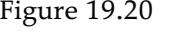
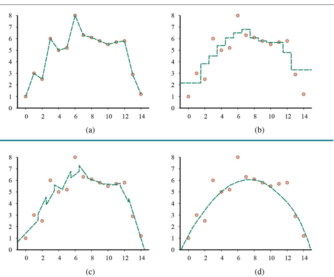
Nonparametric regression models: (a) connect the dots, (b) 3-nearest neighbors average, (c) 3-nearestneighbors linear regression, (d) locally weighted regression with a quadratic kernel of width

-nearest-neighbors regression improves on connect-the-dots. Instead of using just the two examples to the left and right of a query point we use the nearest neighbors. (Here we are using ). A larger value of tends to smooth out the magnitude of the spikes, although the resulting function has discontinuities. Figure 19.20 shows two versions of nearest-neighbors regression. In (b), we have the -nearest-neighbors average: is the

mean value of the points, Notice that at the outlying points, near and the estimates are poor because all the evidence comes from one side (the interior), and ignores the trend. In (c), we have -nearest-neighbor linear regression, which finds the best line through the examples. This does a better job of capturing trends at the outliers, but is still discontinuous. In both (b) and (c), we’re left with the question of how to choose a good value for The answer, as usual, is cross-validation.

Nearest-neighbors regression

Locally weighted regression (Figure 19.20(d) ) gives us the advantages of nearest neighbors, without the discontinuities. To avoid discontinuities in we need to avoid discontinuities in the set of examples we use to estimate The idea of locally weighted regression is that at each query point the examples that are close to are weighted heavily, and the examples that are farther away are weighted less heavily, and the farthest not at all. The decrease in weight over distance is typically gradual, not sudden.

Locally weighted regression

We decide how much to weight each example with a function known as a kernel, whose input is a distance between the query point and the example. A kernel function is a decreasing function of distance with a maximum at 0, so that gives higher weight to examples that are closer to the query point for which we are trying to predict the function value. The integral of the kernel value over the entire input space for must be finite—and if we choose to make the integral 1, certain calculations are easier.

Kernel

Figure 19.20(d) was generated with a quadratic kernel, with kernel width Other shapes, such as Gaussians, are also used. Typically, the width matters more than the exact shape: this is a hyperparameter of the model that is best chosen by cross-validation. If the kernels are too wide we’ll get underfitting and if they are too narrow we’ll get overfitting. In Figure 19.20(d) , a kernel width of 10 gives a smooth curve that looks just about right.

Doing locally weighted regression with kernels is now straightforward. For a given query point we solve the following weighted regression problem:

\[\mathbf{w}^\* = \underset{\mathbf{w}}{\text{argmin}} \sum\_{j} K(Distance(\mathbf{x}\_q, \mathbf{x}\_j)) \left( y\_j - \mathbf{w} \cdot \mathbf{x}\_j \right)^2,\]

where Distance is any of the distance metrics discussed for nearest neighbors. Then the answer is

Note that we need to solve a new regression problem for every query point—that’s what it means to be local. (In ordinary linear regression, we solved the regression problem once, globally, and then used the same for any query point.) Mitigating against this extra work is the fact that each regression problem will be easier to solve, because it involves only the examples with nonzero weight—the examples that are within the kernel width of the query. When kernel widths are small, this may be just a few points.

Most nonparametric models have the advantage that it is easy to do leave-one-out crossvalidation without having to recompute everything. With a -nearest-neighbors model, for instance, when given a test example we retrieve the nearest neighbors once, compute the per-example loss from them, and record that as the leave-one-out result for every example that is not one of the neighbors. Then we retrieve the nearest neighbors and record distinct results for leaving out each of the neighbors. With examples the whole process is not

19.7.5 Support vector machines

In the early 2000s, the support vector machine (SVM) model class was the most popular approach for “off-the-shelf” supervised learning, for when you don’t have any specialized prior knowledge about a domain. That position has now been taken over by deep learning networks and random forests, but SVMs retain three attractive properties:

• 1. SVMs construct a maximum margin separator—a decision boundary with the largest possible distance to example points. This helps them generalize well.
• 2. SVMs create a linear separating hyperplane, but they have the ability to embed the data into a higher-dimensional space, using the so-called kernel trick. Often, data that are not linearly separable in the original input space are easily separable in the higher-dimensional space.
• 3. SVMs are nonparametric—the separating hyperplane is defined by a set of example points, not by a collection of parameter values. But while nearest-neighbor models need to retain all the examples, an SVM model keeps only the examples that are closest to the separating plane—usually only a small constant times the number of dimensions. Thus SVMs combine the advantages of nonparametric and parametric models: they have the flexibility to represent complex functions, but they are resistant to overfitting.

Support vector machine (SVM)

We see in Figure 19.21(a) a binary classification problem with three candidate decision boundaries, each a linear separator. Each of them is consistent with all the examples, so from the point of view of 0/1 loss, each would be equally good. Logistic regression would find some separating line; the exact location of the line depends on all the example points. The key insight of SVMs is that some examples are more important than others, and that paying attention to them can lead to better generalization.

Figure 19.21

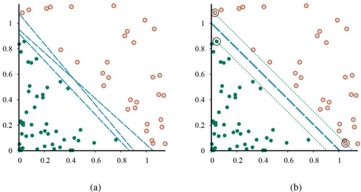
Support vector machine classification: (a) Two classes of points (orange open and green filled circles) and three candidate linear separators. (b) The maximum margin separator (heavy line), is at the midpoint of the margin (area between dashed lines). The support vectors (points with large black circles) are the examples closest to the separator; here there are three.

Consider the lowest of the three separating lines in (a). It comes very close to five of the black examples. Although it classifies all the examples correctly, and thus minimizes loss, it should make you nervous that so many examples are close to the line; it may be that other black examples will turn out to fall on the wrong side of the line.

SVMs address this issue: Instead of minimizing expected empirical loss on the training data, SVMs attempt to minimize expected generalization loss. We don’t know where the as-yetunseen points may fall, but under the probabilistic assumption that they are drawn from the same distribution as the previously seen examples, there are some arguments from computational learning theory (Section 19.5 ) suggesting that we minimize generalization loss by choosing the separator that is farthest away from the examples we have seen so far. We call this separator, shown in Figure 19.21(b) the maximum margin separator. The margin is the width of the area bounded by dashed lines in the figure—twice the distance from the separator to the nearest example point.

Maximum margin separator

Margin

Now, how do we find this separator? Before showing the equations, some notation: Traditionally SVMs use the convention that class labels are and instead of the and 0 we have been using so far. Also, whereas we previously put the intercept into the weight vector (and a corresponding dummy 1 value into ), SVMs do not do that; they keep the intercept as a separate parameter,

With that in mind, the separator is defined as the set of points We could search the space of and with gradient descent to find the parameters that maximize the margin while correctly classifying all the examples.

However, it turns out there is another approach to solving this problem. We won’t show the details, but will just say that there is an alternative representation called the dual representation, in which the optimal solution is found by solving

(19.10)

\[\underset{\alpha}{\text{argmax}} \sum\_{j} \alpha\_{j} - \frac{1}{2} \sum\_{j,k} \alpha\_{j} \alpha\_{k} y\_{j} y\_{k} (\mathbf{x}\_{j} \cdot \mathbf{x}\_{k})^{2}\]

Quadratic programming

subject to the constraints and This is a quadratic programming optimization problem, for which there are good software packages. Once we have found the vector we can get back to with the equation or we can stay in the dual representation. There are three important properties of Equation (19.10) . First, the expression is convex; it has a single global maximum that can be found efficiently. Second, the data enter the expression only in the form of dot products of pairs of points. This second property is also true of the equation for the separator itself; once the optimal have been calculated, the equation is 11

11 The function returns for a positive for a negative

(19.11)

\[h(\mathbf{x}) = \text{sign}\left(\sum\_{j} \alpha\_{j} y\_{j}(\mathbf{x} \cdot \mathbf{x}\_{j}) - b\right).\]

A final important property is that the weights associated with each data point are zero except for the support vectors—the points closest to the separator. (They are called “support” vectors because they “hold up” the separating plane.) Because there are usually many fewer support vectors than examples, SVMs gain some of the advantages of parametric models.

Support vector

What if the examples are not linearly separable? Figure 19.22(a) shows an input space defined by attributes with positive examples inside a circular region and negative examples outside. Clearly, there is no linear separator for this problem. Now, suppose we re-express the input data—that is, we map each input vector to a new vector of feature values, In particular, let us use the three features

(19.12)

\[f\_1 = x\_1^2, \qquad f\_2 = x\_2^2, \qquad f\_3 = \sqrt{2}x\_1x\_2.\]

Figure 19.22

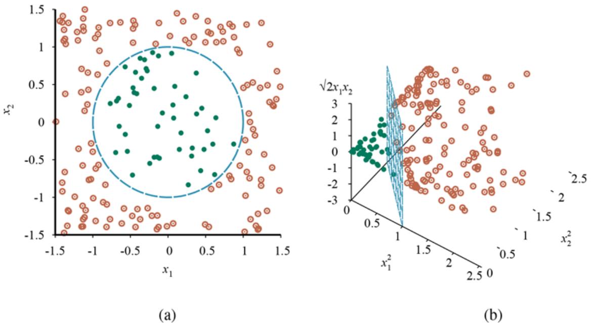
1. A two-dimensional training set with positive examples as green filled circles and negative examples as orange open circles. The true decision boundary, is also shown. (b) The same data after mapping into a three-dimensional input space The circular decision boundary in (a) becomes a linear decision boundary in three dimensions. Figure 19.21(b) gives a closeup of the separator in (b).

We will see shortly where these came from, but for now, just look at what happens. Figure 19.22(b) shows the data in the new, three-dimensional space defined by the three features; the data are linearly separable in this space! This phenomenon is actually fairly general: if data are mapped into a space of sufficiently high dimension, then they will almost always be linearly separable—if you look at a set of points from enough directions, you’ll find a way to make them line up. Here, we used only three dimensions; Exercise 19.SVME asks you to show that four dimensions suffice for linearly separating a circle anywhere in the plane (not just at the origin), and five dimensions suffice to linearly separate any ellipse. In general (with some special cases excepted) if we have data points then they will always be separable in spaces of dimensions or more (Exercise 19.EMBE). 12

12 The reader may notice that we could have used just and but the 3D mapping illustrates the idea better.

Now, we would not usually expect to find a linear separator in the input space but we can find linear separators in the high-dimensional feature space simply by replacing in Equation (19.10) with This by itself is not remarkable—replacing by in any learning algorithm has the required effect—but the dot product has some special properties. It turns out that can often be computed without first computing

for each point. In our three-dimensional feature space defined by Equation (19.12) , a little bit of algebra shows that

\[F(\mathbf{x}\_j) \cdot F(\mathbf{x}\_k) = (\mathbf{x}\_j \cdot \mathbf{x}\_k)^2.\]

(That’s why the is in ) The expression is called a kernel function, and is usually written as The kernel function can be applied to pairs of input data to evaluate dot products in some corresponding feature space. So, we can find linear separators in the higher-dimensional feature space simply by replacing in Equation (19.10) with a kernel function Thus, we can learn in the higherdimensional space, but we compute only kernel functions rather than the full list of features for each data point. 13

13 This usage of “kernel function” is slightly different from the kernels in locally weighted regression. Some SVM kernels are distance metrics, but not all are.

Kernel function

The next step is to see that there’s nothing special about the kernel It corresponds to a particular higher-dimensional feature space, but other kernel functions correspond to other feature spaces. A venerable result in mathematics, Mercer’s theorem (1909), tells us that any “reasonable” kernel function corresponds to some feature space. These feature spaces can be very large, even for innocuous-looking kernels. For example, the polynomial kernel, corresponds to a feature space whose dimension is exponential in A common kernel is the Gaussian: 14

14 Here, “reasonable” means that the matrix is positive definite.

Mercer’s theorem

19.7.6 The kernel trick

This then is the clever kernel trick: Plugging these kernels into Equation (19.10) , optimal linear separators can be found efficiently in feature spaces with billions of (or even infinitely many) dimensions. The resulting linear separators, when mapped back to the original input space, can correspond to arbitrarily wiggly, nonlinear decision boundaries between the positive and negative examples.

Kernel trick

In the case of inherently noisy data, we may not want a linear separator in some highdimensional space. Rather, we’d like a decision surface in a lower-dimensional space that does not cleanly separate the classes, but reflects the reality of the noisy data. That is possible with the soft margin classifier, which allows examples to fall on the wrong side of the decision boundary, but assigns them a penalty proportional to the distance required to move them back to the correct side.

Soft margin

The kernel method can be applied not only with learning algorithms that find optimal linear separators, but also with any other algorithm that can be reformulated to work only with dot products of pairs of data points, as in Equations (19.10) and (19.11) . Once this is done, the dot product is replaced by a kernel function and we have a kernelized version of the algorithm.

Kernelization

19.8 Ensemble Learning

So far we have looked at learning methods in which a single hypothesis is used to make predictions. The idea of ensemble learning is to select a collection, or ensemble, of hypotheses, and combine their predictions by averaging, voting, or by another level of machine learning. We call the individual hypotheses base models and their combination an ensemble model.

Ensemble learning

Base model

Ensemble model

There are two reasons to do this. The first is to reduce bias. The hypothesis space of a base model may be too restrictive, imposing a strong bias (such as the bias of a linear decision boundary in logistic regression). An ensemble can be more expressive, and thus have less bias, than the base models. Figure 19.23 shows that an ensemble of three linear classifiers can represent a triangular region that could not be represented by a single linear classifier. An ensemble of linear classifiers allows more functions to be realizable, at a cost of only times more computation; this is often better than allowing a completely general hypothesis space that might require exponentially more computation.

Figure 19.23

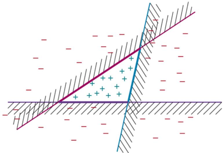
Illustration of the increased expressive power obtained by ensemble learning. We take three linear threshold hypotheses, each of which classifies positively on the unshaded side, and classify as positive any example classified positively by all three. The resulting triangular region is a hypothesis not expressible in the original hypothesis space.

The second reason is to reduce variance. Consider an ensemble of binary classifiers that we combine using majority voting. For the ensemble to misclassify a new example, at least three of the five classifiers have to misclassify it. The hope is that this is less likely than a single misclassification by a single classifier. To quantify that, suppose you have trained a single classifier that is correct in 80% of cases. Now create an ensemble of 5 classifiers, each trained on a different subset of the data so that they are independent. Let’s assume this leads to some reduction in quality, and each individual classifier is correct in only 75% of cases. But together, the majority vote of the ensemble will be correct in 89% of cases (and 99% with 17 classifiers), assuming true independence.

In practice the independence assumption is unreasonable—individual classifiers share some of the same data and assumptions, and thus are not completely independent, and will share some of the same errors. But if the component classifiers are at least somewhat uncorrelated then ensemble learning will make fewer misclassifications. We will now consider four ways of creating ensembles: bagging, random forests, stacking, and boosting.

19.8.1 Bagging

In bagging, we generate distinct training sets by sampling with replacement from the original training set. That is, we randomly pick examples from the training set, but each of those picks might be an example we picked before. We then run our machine learning 15

algorithm on the examples to get a hypothesis. We repeat this process times, getting different hypotheses. Then, when asked to predict the value of a new input, we aggregate the predictions from all hypotheses. For classification problems, that means taking the plurality vote (the majority vote for binary classification). For regression problems, the final output is the average:

15 Note on terminology: In statistics, a sample with replacement is called a bootstrap, and “bagging” is short for “bootstrap aggregating.”

\[h(\mathbf{x}) = \frac{1}{K} \sum\_{i=1}^{K} h\_i(\mathbf{x})\]

Bagging

Bagging tends to reduce variance and is a standard approach when there is limited data or when the base model is seen to be overfitting. Bagging can be applied to any class of model, but is most commonly used with decision trees. It is appropriate because decision trees are unstable: a slightly different set of examples can lead to a wildly different tree. Bagging smoothes out this variance. If you have access to multiple computers then bagging is efficient, because the hypotheses can be computed in parallel.

19.8.2 Random forests

Unfortunately, bagging decision trees often ends up giving us trees that are highly correlated. If there is one attribute with a very high information gain, it is likely to be the root of most of the trees. The random forest model is a form of decision tree bagging in which we take extra steps to make the ensemble of trees more diverse, to reduce variance. Random forests can be used for classification or regression.

Random forests

The key idea is to randomly vary the attribute choices (rather than the training examples). At each split point in constructing the tree, we select a random sampling of attributes, and then compute which of those gives the highest information gain. If there are attributes, a common default choice is that each split randomly picks attributes to consider for classification problems, or for regression problems.

A further improvement is to use randomness in selecting the split point value: for each selected attribute, we randomly sample several candidate values from a uniform distribution over the attribute’s range. Then we select the value that has the highest information gain. That makes it more likely that every tree in the forest will be different. Trees constructed in this fashion are called extremely randomized trees (ExtraTrees).

Extremely randomized trees (ExtraTrees)

Random forests are efficient to create. You might think that it would take times longer to create an ensemble of trees, but it is not that bad, for three reasons: (a) each split point runs faster because we are considering fewer attributes, (b) we can skip the pruning step for each individual tree, because the ensemble as a whole decreases overfitting, and (c) if we happen to have computers available, we can build all the trees in parallel. For example, Adele Cutler reports that for a 100-attribute problem, if we have just three CPUs we can grow a forest of trees in about the same time as it takes to create a single decision tree on a single CPU.

All the hyperparameters of random forests can be trained by cross-validation: the number of trees the number of examples used by each tree (often expressed as a percentage of the complete data set), the number of attributes used at each split point (often expressed as a function of the total number of attributes, such as ), and the number of random split points tried if we are using ExtraTrees. In place of the regular cross-validation strategy, we could measure the out-of-bag error: the mean error on each example, using only the trees whose example set didn’t include that particular example.

Out-of-bag error

We have been warned that more complex models can be prone to overfitting, and observed that to be true for decision trees, where we found that pruning was an answer to prevent overfitting. Random forests are complex, unpruned models. Yet they are resistant to overfitting. As you increase capacity by adding more trees to the forest they tend to improve on validation-set error rate. The curve typically looks like Figure 19.9(b) , not (a) .

Breiman (2001) gives a mathematical proof that (in almost all cases) as you add more trees to the forest, the error converges; it does not grow. One way to think of it is that the random selection of attributes yields a variety of trees, thus reducing variance, but because we don’t need to prune the trees, they can cover the full input space at higher resolution. Some number of trees can cover unique cases that appear only a few times in the data, and their votes can prove decisive, but they can be outvoted when they do not apply. That said, random forests are not totally immune to overfitting. Although the error can’t increase in the limit, that does not mean that the error will go to zero.

Random forests have been very successful across a wide variety of application problems. In Kaggle data science competitions they were the most popular approach of winning teams from 2011 through 2014, and remain a common approach to this day (although deep learning and gradient boosting have become even more common among recent winners). The randomForest package in R has been a particular favorite. In finance, random forests have been used for credit card default prediction, household income prediction, and option pricing. Mechanical applications include machine fault diagnosis and remote sensing. Bioinformatic and medical applications include diabetic retinopathy, microarray gene expression, mass spectrum protein expression analysis, biomarker discovery, and protein– protein interaction prediction.

19.8.3 Stacking

Whereas bagging combines multiple base models of the same model class trained on different data, the technique of stacked generalization (or stacking for short) combines multiple base models from different model classes trained on the same data. For example, suppose we are given the restaurant data set, the first row of which is shown here:

Stacked generalization

We separate the data into training, validation, and test sets and use the training set to train, say, three separate base models—an SVM model, a logistic regression model, and a decision tree model.

In the next step we take the validation data set and augment each row with the predictions made from the three base models, giving us rows that look like this (where the predictions are shown in bold):

\[\mathbf{x}\_2 = \text{Yes, No, No, Yes,Full, \\$, No, No, No, Then, 30 - 60, \textbf{Yes, No, No}; \textbf{No}; \textbf{y}\_2 = \text{No}\]

We use this validation set to train a new ensemble model, let’s say a logistic regression model (but it need not be one of the base model classes). The ensemble model can use the predictions and the original data as it sees fit. It might learn a weighted average of the base models, for example that the predictions should be weighted in a ratio of 50%:30%:20%. Or it might learn nonlinear interactions between the data and the predictions, perhaps trusting the SVM model more when the wait time is long, for example. We used the same training data to train each of the base models, and then used the held-out validation data (plus predictions) to train the ensemble model. It is also possible to use cross-validation if desired.

The method is called “stacking” because it can be thought of as a layer of base models with an ensemble model stacked above it, operating on the output of the base models. In fact, it is possible to stack multiple layers, each one operating on the output of the previous layer. Stacking reduces bias, and usually leads to performance that is better than any of the individual base models. Stacking is frequently used by winning teams in data science competitions (such as Kaggle and the KDD Cup), because individuals can work independently, each refining their own base model, and then come together to build the final stacked ensemble model.

19.8.4 Boosting

The most popular ensemble method is called boosting. To understand how it works, we need first to introduce the idea of a weighted training set, in which each example has an associated weight that describes how much the example should count during training. For example, if one example had a weight of 3 and the other examples all had a weight of 1, that would be equivalent to having 3 copies of the one example in the training set.

Boosting

Weighted training set

Boosting starts with equal weights for all the examples. From this training set, it generates the first hypothesis, In general, will classify some of the training examples correctly and some incorrectly. We would like the next hypothesis to do better on the misclassified examples, so we increase their weights while decreasing the weights of the correctly classified examples.

From this new weighted training set, we generate hypothesis The process continues in this way until we have generated hypotheses, where is an input to the boosting algorithm. Examples that are difficult to classify will get increasingly larger weights until the algorithm is forced to create a hypothesis that classifies them correctly. Note that this is a greedy algorithm in the sense that it does not backtrack; once it has chosen a hypothesis it will never undo that choice; rather it will add new hypotheses. It is also a sequential algorithm, so we can’t compute all the hypotheses in parallel as we could with bagging.

The final ensemble lets each hypothesis vote, as in bagging, except that each hypothesis gets a weighted number of votes—the hypotheses that did better on their respective weighted training sets are given more voting weight. For regression or binary classification we have

\[h(\mathbf{x}) = \sum\_{i=1}^{K} z\_i h\_i(\mathbf{x})\]

where is the weight of the th hypothesis. (This weighting of hypotheses is distinct from the weighting of examples.)

Figure 19.24 shows how the algorithm works conceptually. There are many variants of the basic boosting idea, with different ways of adjusting the example weights and combining the hypotheses. The variants all share the general idea that difficult examples get more weight as we move from one hypothesis to the next. Like the Bayesian learning methods we will see in Chapter 20 , they also give more weight to more accurate hypotheses.

Figure 19.24

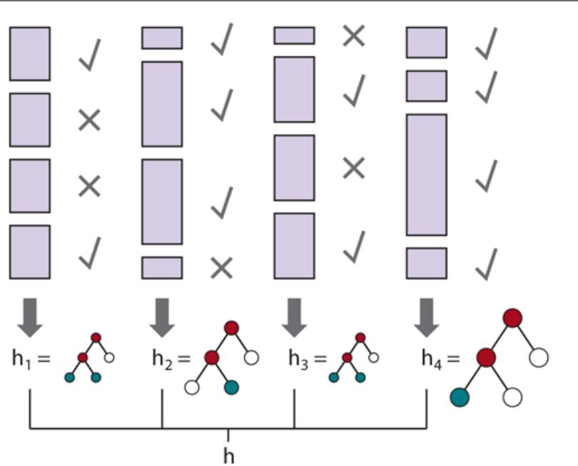
How the boosting algorithm works. Each shaded rectangle corresponds to an example; the height of the rectangle corresponds to the weight. The checks and crosses indicate whether the example was classified correctly by the current hypothesis. The size of the decision tree indicates the weight of that hypothesis in the final ensemble.

One specific algorithm, called ADABOOST, is shown in Figure 19.25 . It is usually applied with decision trees as the component hypotheses; often the trees are limited in size. ADABOOST has a very important property: if the input learning algorithm is a weak learning algorithm—which means that always returns a hypothesis with accuracy on the training set that is slightly better than random guessing (that is, 50% for Boolean

classification)—then ADABOOST will return a hypothesis that classifies the training data perfectly for large enough Thus, the algorithm boosts the accuracy of the original learning algorithm on the training data.

Figure 19.25

The ADABOOST variant of the boosting method for ensemble learning. The algorithm generates hypotheses by successively reweighting the training examples. The function WEIGHTED-MAJORITY generates a hypothesis that returns the output value with the highest vote from the hypotheses in with votes weighted by For regression problems, or for binary classification with two classes and 1, this is

Weak learning

In other words, boosting can overcome any amount of bias in the base model, as long as the base model is better than random guessing. (In our pseudocode we stop generating

hypotheses if we get one that is worse than random.) This result holds no matter how inexpressive the original hypothesis space and no matter how complex the function being learned. The exact formulas for weights in Figure 19.25 (with etc.) are chosen to make the proof of this property easy (see (Freund and Schapire, 1996)). Of course, this property does not guarantee accuracy on previously unseen examples.

Let us see how well boosting does on the restaurant data. We will choose as our original hypothesis space the class of decision stumps, which are decision trees with just one test, at the root. The lower curve in Figure 19.26(a) shows that unboosted decision stumps are not very effective for this data set, reaching a prediction performance of only 81% on 100 training examples. When boosting is applied (with ), the performance is better, reaching 93% after 100 examples.

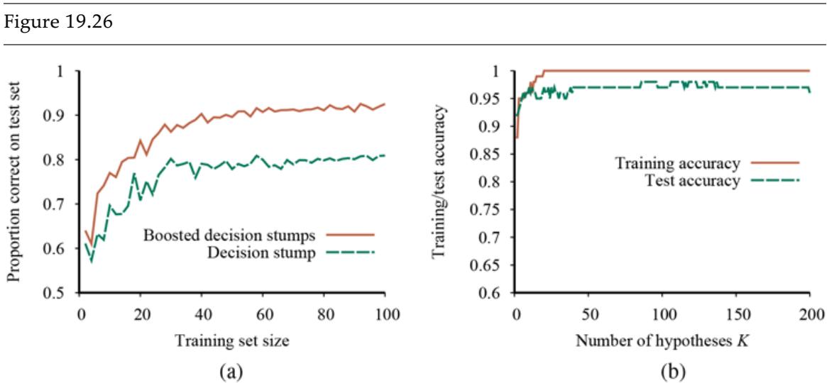
1. Graph showing the performance of boosted decision stumps with versus unboosted decision stumps on the restaurant data. (b) The proportion correct on the training set and the test set as a function of the number of hypotheses in the ensemble. Notice that the test set accuracy improves slightly even after the training accuracy reaches 1, i.e., after the ensemble fits the data exactly.

Decision stump

An interesting thing happens as the ensemble size increases. Figure 19.26(b) shows the training set performance (on 100 examples) as a function of Notice that the error reaches zero when is 20; that is, a weighted-majority combination of 20 decision stumps suffices to fit the 100 examples exactly—this is the interpolation pont. As more stumps are added to the ensemble, the error remains at zero. The graph also shows that the test set performance continues to increase long after the training set error has reached zero. At the test performance is 0.95 (or 0.05 error), and the performance increases to 0.98 as late as before gradually dropping to 0.95.

This finding, which is quite robust across data sets and hypothesis spaces, came as quite a surprise when it was first noticed. Ockham’s razor tells us not to make hypotheses more complex than necessary, but the graph tells us that the predictions improve as the ensemble hypothesis gets more complex! Various explanations have been proposed for this. One view is that boosting approximates Bayesian learning (see Chapter 20 ), which can be shown to be an optimal learning algorithm, and the approximation improves as more hypotheses are added. Another possible explanation is that the addition of further hypotheses enables the ensemble to be more confident in its distinction between positive and negative examples, which helps it when it comes to classifying new examples.

19.8.5 Gradient boosting

For regression and classification of factored tabular data, gradient boosting, sometimes called gradient boosting machines (GBM) or gradient boosted regression trees (GBRT), has become a very popular method. As the name implies, gradient boosting is a form of boosting using gradient descent. Recall that in ADABOOST, we start with one hypothesis and boost it with a sequence of hypotheses that pay special attention to the examples that the previous ones got wrong. In gradient boosting we also add new boosting hypotheses, which pay attention not to specific examples, but to the gradient between the right answers and the answers given by the previous hypotheses.

Gradient boosting

As in the other algorithms that used gradient descent, we start with a differentiable loss function; we might use squared error for regression, or logarithmic loss for classification. As in ADABOOST, we then build a decision tree. In Section 19.6.2 , we used gradient descent to

minimize the parameters of a model—we calculate the loss, and update the parameters in the direction of less loss. With gradient boosting, we are not updating parameters of the existing model, we are updating the parameters of the next tree—but we must do that in a way that reduces the loss by moving in the right direction along the gradient.

As in the models we saw in Section 19.4.3 , regularization can help prevent overfitting. That can come in the form of limiting the number of trees or their size (in terms of their depth or number of nodes). It can come from the learning rate, which says how far to move along the direction of the gradient; values in the range 0.1 to 0.3 are common, and the smaller the learning rate, the more trees we will need in the ensemble.

Gradient boosting is implemented in the popular XGBOOST (eXtreme Gradient Boosting) package, which is routinely used for both large-scale applications in industry (for problems with billions of examples), and by the winners of data science competitions (in 2015, it was used by every team in the top 10 of the KDDCup). XGBOOST does gradient boosting with pruning and regularization, and takes care to be efficient, carefully organizing memory to avoid cache misses, and allowing for parallel computation on multiple machines.

19.8.6 Online learning

So far, everything we have done in this chapter has relied on the assumption that the data are i.i.d. (independent and identically distributed). On the one hand, that is a sensible assumption: if the future bears no resemblance to the past, then how can we predict anything? On the other hand, it is too strong an assumption: we know that there are correlations between the past and the future, and in complex scenarios it is unlikely that we will capture all the data that would make the future independent of the past given the data.

In this section we examine what to do when the data are not i.i.d.—when they can change over time. In this case, it matters when we make a prediction, so we will adopt the perspective called online learning: an agent receives an input from nature, predicts the corresponding and then is told the correct answer. Then the process repeats with and so on. One might think this task is hopeless—if nature is adversarial, all the predictions may be wrong. It turns out that there are some guarantees we can make.

Online learning

Let us consider the situation where our input consists of predictions from a panel of experts. For example, each day pundits predict whether the stock market will go up or down, and our task is to pool those predictions and make our own. One way to do this is to keep track of how well each expert performs, and choose to believe them in proportion to their past performance. This is called the randomized weighted majority algorithm. We can describe it more formally:

Initialize a set of weights all to 1.

for each problem to be solved do

• 1. Receive the predictions from the experts.
• 2. Randomly choose an expert in proportion to its weight:
• 3. yield as the answer to this problem.
• 4. Receive the correct answer
• 5. For each expert such that update
• 6. Normalize the weights so that

Randomized weighted majority algorithm

Here is a number, that tells how much to penalize an expert for each mistake.

We measure the success of this algorithm in terms of regret, which is defined as the number of additional mistakes we make compared to the expert who, in hindsight, had the best prediction record. Let be the number of mistakes made by the best expert. Then the number of mistakes, made by the random weighted majority algorithm, is bounded by 16

\[M < \frac{M^\* \ln(1/\beta) + \ln K}{1 - \beta}.\]

Regret

This bound holds for any sequence of examples, even ones chosen by adversaries trying to do their worst. To be specific, when there are experts, if we choose then our number of mistakes is bounded by and if by In general, if is close to 1 then we are responsive to change over the long run; if the best expert changes, we will pick up on it before too long. However, we pay a penalty at the beginning, when we start with all experts trusted equally; we may accept the advice of the bad experts for too long. When is closer to 0, these two factors are reversed. Note that we can choose so that gets asymptotically close to in the long run; this is called no-regret learning (because the average amount of regret per trial tends to 0 as the number of trials increases).

No-regret learning

Online learning is helpful when the data may be changing rapidly over time. It is also useful for applications that involve a large collection of data that is constantly growing, even if changes are gradual. For example, with a data set of millions of Web images, you wouldn’t want to retrain from scratch every time a single new image is added. It would be more practical to have an online algorithm that allows images to be added incrementally. For most learning algorithms based on minimizing loss, there is an online version based on minimizing regret. Many of these online algorithms come with guaranteed bounds on regret.

It may seem surprising that there are such tight bounds on how well we can do compared to a panel of experts. What is even more surprising is that when such panels convene to prognosticate about political contests or sporting events, the viewing public is so willing to listen to their predictions and so uninterested in knowing their error rates.

19.9 Developing Machine Learning Systems

In this chapter we have concentrated on explaining the theory of machine learning. The practice of using machine learning to solve practical problems is a separate discipline. Over the last 50 years, the software industry has evolved a software development methodology that makes it more likely that a (traditional) software project will be a success. But we are still in the early stages of defining a methodology for machine learning projects; the tools and techniques are not as well-developed. Here is a breakdown of typical steps in the process.

19.9.1 Problem formulation

The first step is to figure out what problem you want to solve. There are two parts to this. First ask, “what problem do I want to solve for my users?” An answer such as “make it easier for users to organize and access their photos” is too vague; “help a user find all photos that match a specific term, such as Paris” is better. Then ask, “what part(s) of the problem can be solved by machine learning?” perhaps settling on “learn a function that maps a photo to a set of labels; then, when given a label as a query, retrieve all photos with that label.”

To make this concrete, you need to specify a loss function for your machine learning component, perhaps measuring the system’s accuracy at predicting a correct label. This objective should be correlated with your true goals, but usually will be distinct—the true goal might be to maximize the number of users you gain and keep on your system, and the revenue that they produce. Those are metrics you should track, but not necessarily ones that you can directly build a machine learning model for.

When you have decomposed your problem into parts, you may find that there are multiple components that can be handled by old-fashioned software engineering, not machine learning. For example, for a user who asks for “best photos,” you could implement a simple procedure that sorts photos by the number of likes and views. Once you have developed your overall system to the point where it is viable, you can then go back and optimize, replacing the simple components with more sophisticated machine learning models.

Part of problem formulation is deciding whether you are dealing with supervised, unsupervised, or reinforcement learning. The distinctions are not always so crisp. In semisupervised learning we are given a few labeled examples and use them to mine more information from a large collection of unlabeled examples. This has become a common approach, with companies emerging whose missions are to quickly label some examples, in order to help machine learning systems make better use of the remaining unlabeled examples.

Semisupervised learning

Sometimes you have a choice of which approach to use. Consider a system to recommend songs or movies to customers. We could approach this as a supervised learning problem, where the inputs include a representation of the customer and the labeled output is whether or not they liked the recommendation, or we could approach it as a reinforcement learning problem, where the system makes a series of recommendation actions, and occasionally gets a reward from the customer for making a good suggestion.

The labels themselves may not be the oracular truths that we hope for. Imagine that you are trying to build a system to guess a person’s age from a photo. You gather some labeled examples by having people upload photos and state their age. That’s supervised learning. But in reality some of the people lied about their age. It’s not just that there is random noise in the data; rather the inaccuracies are systematic, and to uncover them is an unsupervised learning problem involving images, self-reported ages, and true (unknown) ages. Thus, both noise and lack of labels create a continuum between supervised and unsupervised learning. The field of weakly supervised learning focuses on using labels that are noisy, imprecise, or supplied by non-experts.

Weakly supervised learning

19.9.2 Data collection, assessment, and management

Every machine learning project needs data; in the case of our photo identification project there are freely available image data sets, such as ImageNet, which has over 14 million photos with about 20,000 different labels. Sometimes we may have to manufacture our own data, which can be done by our own labor, or by crowdsourcing to paid workers or unpaid volunteers operating over an Internet service. Sometimes data come from your users. For example, the Waze navigation service encourages users to upload data about traffic jams, and uses that to provide up-to-date navigation directions for all users. Transfer learning (see Section 21.7.2 ) can be used when you don’t have enough of your own data: start with a publicly available general-purpose data set (or a model that has been pretrained on this data), and then add specific data from your users and retrain.

ImageNet

If you deploy a system to users, your users will provide feedback—perhaps by clicking on one item and ignoring the others. You will need a strategy for dealing with this data. That involves a review with privacy experts (see Section 27.3.2 ) to make sure that you get the proper permission for the data you collect, and that you have processes for insuring the integrity of the user’s data, and that they understand what you will do with it. You also need to ensure that your processes are fair and unbiased (see Section 27.3.3 ). If there is data that you feel is too sensitive to collect but that would be useful for a machine learning model, consider a federated learning approach where the data stays on the user’s device, but model parameters are shared in a way that does not reveal private data.

It is good practice to maintain data provenance for all your data. For each column in your data set, you should know the exact definition, where the data come from, what the possible values are, and who has worked on it. Were there periods of time in which a data feed was interrupted? Did the definition of some data source evolve over time? You’ll need to know this if you want to compare results across time periods.

Data provenance

This is particularly true if you are relying on data that are produced by someone else—their needs and yours might diverge, and they might end up changing the way the data are produced, or might stop updating it all together. You need to monitor your data feeds to catch this. Having a reliable, flexible, secure, data-handling pipeline is more critical to success than the exact details of the machine learning algorithm. Provenance is also important for legal reasons, such as compliance with privacy law.

For any task there will be questions about the data: Is this the right data for my task? Does it capture enough of the right inputs to give us a chance of learning a model? Does it contain the outputs I want to predict? If not, can I build an unsupervised model? Or can I label a portion of the data and then do semisupervised learning? Is it relevant data? It is great to have 14 million photos, but if all your users are specialists interested in a specific topic, then a general database won’t help—you’ll need to collect photos on the specific topic. How much training data is enough? (Do I need to collect more data? Can I discard some data to make computation faster?) The best way to answer this is to reason by analogy to a similar project with known training set size.

Once you get started you can draw a learning curve (see Figure 19.7 ) to see if more data will help, or if learning has already plateaued. There are endless ad hoc, unjustified rules of thumb for the number of training examples you’ll need: millions for hard problems; thousands for average problems; hundreds or thousands for each class in a classification problem; 10 times more examples than parameters of the model; 10 times more examples than input features; examples for input features; more examples for nonlinear models than for linear models; more examples if greater accuracy is required; fewer examples if you use regularization; enough examples to achieve the statistical power necessary to reject the null hypothesis in classification. All these rules come with caveats—as does the sensible rule that suggests trying what has worked in the past for similar problems.

You should think defensively about your data. Could there be data entry errors? What can be done with missing data fields? If you collect data from your customers (or other people) could some of the people be adversaries out to game the system? Are there spelling errors or inconsistent terminology in text data? (For example, do “Apple,” “AAPL,” and “Apple Inc.” all refer to the same company?) You will need a process to catch and correct all these potential sources of data error.

When data are limited, data augmentation can help. For example, with a data set of images, you can create multiple versions of each image by rotating, translating, cropping, or scaling each image, or by changing the brightness or color balance or adding noise. As long as these are small changes, the image label should remain the same, and a model trained on such augmented data will be more robust.

Data augmentation

Sometimes data are plentiful but are classified into unbalanced classes. For example, a training set of credit card transactions might consist of 10,000,000 valid transactions and 1,000 fraudulent ones. A classifier that says “valid” regardless of the input will achieve 99.99% accuracy on this data set. To go beyond that, a classifier will have to pay more attention to the fraudulent examples. To help it do that, you can undersample the majority class (i.e., ignore some of the “valid” class examples) or over-sample the minority class (i.e., duplicate some of the “fraudulent” class examples). You can use a weighted loss function that gives a larger penalty to missing a fraudulent case.

Unbalanced classes

Undersampling

Over-sample

Boosting can also help you focus on the minority class. If you are using an ensemble method, you can change the rules by which the ensemble votes and give “fraudulent” as the response even if only a minority of the ensemble votes for “fraudulent.” You can help balance unbalanced classes by generating synthetic data with techniques such as SMOTE (Chawla et al., 2002) or ADASYN (He et al., 2008).

You should carefully consider outliers in your data. An outlier is a data point that is far from other points. For example, in the restaurant problem, if price were a numeric value rather than a categorical one, and if one example had a price of while all the others were 30 or less, that example would be an outlier. Methods such as linear regression are susceptible to outliers because they must form a single global linear model that takes all inputs into account—they can’t treat the outlier differently from other example points, and thus a single outlier can have a large effect on all the parameters of the model.

Outlier

With attributes like price that are positive numbers, we can diminish the effect of outliers by transforming the data, taking the logarithm of each value, so and become 1.3, 1.4, and 2.5. This makes sense from a practical point of view because the high value now has less influence on the model, and from a theoretical point of view because, as we saw in Section 16.3.2 , the utility of money is logarithmic.

Methods such as decision trees that are built from multiple local models can treat outliers individually: it doesn’t matter if the biggest value is or either way it can be treated in its own local node after a test of the form That makes decision trees (and thus random forests and gradient boosting) more robust to outliers.

Feature engineering

After correcting overt errors, you may also want to preprocess your data to make it easier to digest. We have already seen the process of quantization: forcing a continuous valued input, such as the wait time, into fixed bins Domain knowledge can tell you what thresholds are important, such as comparing when

studying voting patterns. We also saw (page 688 ) that nearest-neighbor algorithms perform better when data are normalized to have a standard deviation of 1. With categorical attributes such as sunny/cloudy/rainy, it is often helpful to transform the data into three separate Boolean attributes, exactly one of which is true (we call this a one-hot encoding). This is particularly useful when the machine learning model is a neural network.

One-hot encoding

You can also introduce new attributes based on your domain knowledge. For example, given a data set of customer purchases where each entry has a date attribute, you might want to augment the data with new attributes saying whether the date is a weekend or holiday.

As another example, consider the task of estimating the true value of houses that are for sale. In Figure 19.13 we showed a toy version of this problem, doing linear regression of house size to asking price. But we really want to estimate the selling price of a house, not the asking price. To solve this task we’ll need data on actual sales. But that doesn’t mean we should throw away the data about asking price—we can use it as one of the input features. Besides the size of the house, we’ll need more information: the number of rooms, bedrooms, and bathrooms; whether the kitchen and bathrooms have been recently remodeled; the age of the house and perhaps its state of repair; whether it has central heating and air conditioning; the size of the yard and the state of the landscaping.

We’ll also need information about the lot and the neighborhood. But how do we define neighborhood? By zip code? What if a zip code straddles a desirable and an undesirable neighborhood? What about the school district? Should the name of the school district be a feature, or the average test scores? The ability to do a good job of feature engineering is critical to success. As Pedro Domingos (2012) says, “At the end of the day, some machine learning projects succeed and some fail. What makes the difference? Easily the most important factor is the features used.”

Exploratory data analysis and visualization

John Tukey (1977) coined the term exploratory data analysis (EDA) for the process of exploring data in order to gain an understanding of it, not to make predictions or test hypotheses. This is done mostly with visualizations, but also with summary statistics. Looking at a few histograms or scatter plots can often help determine if data are missing or erroneous; whether your data are normally distributed or heavy-tailed; and what learning model might be appropriate.

It can be helpful to cluster your data and then visualize a prototype data point at the center of each cluster. For example, in the data set of images, I can identify that here is a cluster of cat faces; nearby is a cluster of sleeping cats; other clusters depict other objects. Expect to iterate several times between visualizing and modeling—to create clusters you need a distance function to tell you which items are near each other, but to choose a good distance function you need some feel for the data.

It is also helpful to detect outliers that are far from the prototypes; these can be considered critics of the prototype model, and can give you a feel for what type of errors your system might make. An example would be a cat wearing a lion costume.

Our computer display devices (screens or paper) are two-dimensional, which means that it is easy to visualize two-dimensional data. And our eyes are experienced at understanding three-dimensional data that has been projected down to two dimensions. But many data sets have dozens or even millions of dimensions. In order to visualize them we can do dimensionality reduction, projecting the data down to a map in two dimensions (or sometimes to three dimensions, which can then be explored interactively). 17

17 Geoffrey Hinton provides the helpful advice “To deal with a 14-dimensional space, visualize a 3D space and say ‘fourteen’ to yourself very loudly.”

The map can’t maintain all relationships between data points, but should have the property that similar points in the original data set are close together in the map. A technique called t-distributed stochastic neighbor embedding (t-SNE) does just that. Figure 19.27 shows a t-SNE map of the MNIST digit recognition data set. Data analysis and visualization packages such as Pandas, Bokeh, and Tableau can make it easier to work with your data.

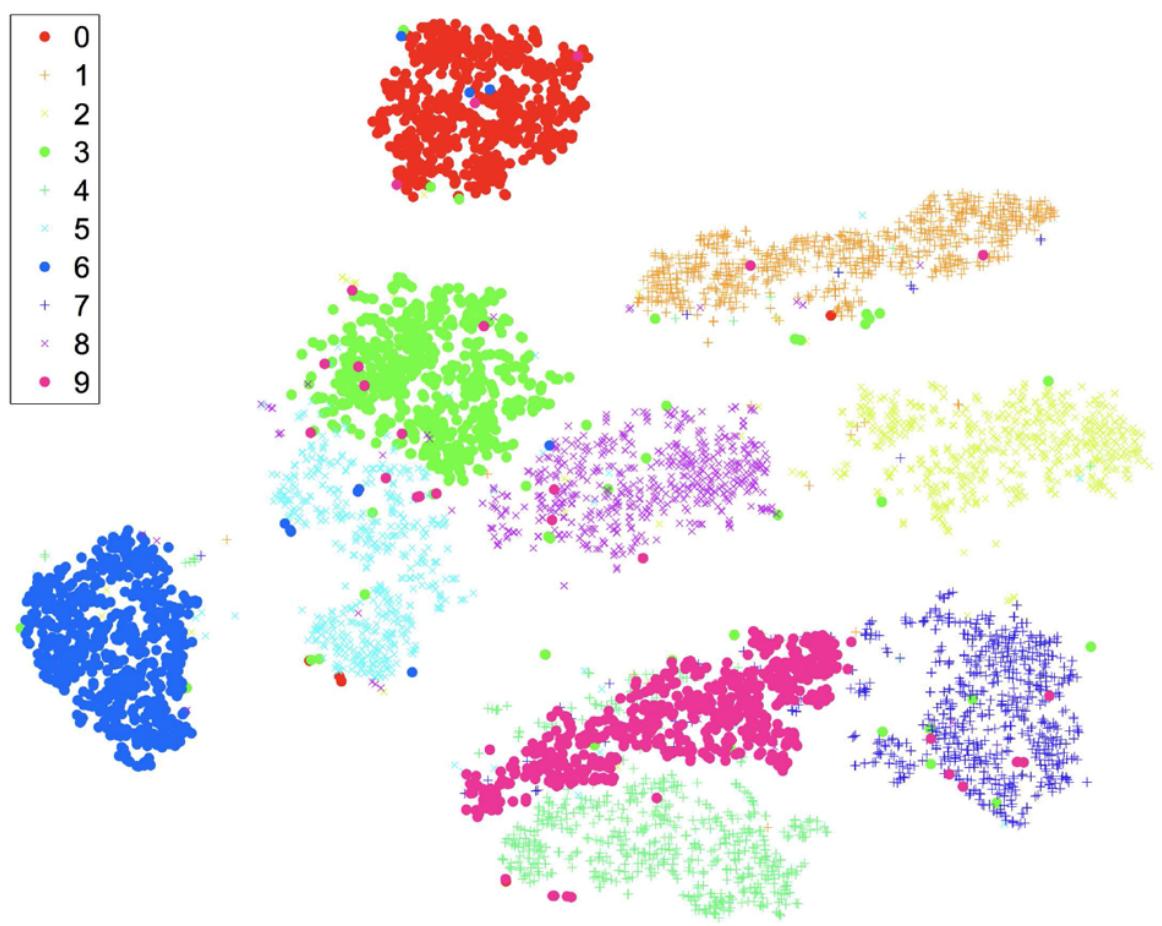
A two-dimensional t-SNE map of the MNIST data set, a collection of 60,000 images of handwritten digits, each pixels and thus 784 dimensions. You can clearly see clusters for the ten digits, with a few confusions in each cluster; for example the top cluster is for the digit 0, but within the bounds of the cluster are a few data points representing the digits 3 and 6. The t-SNE algorithm finds a representation that accentuates the differences between clusters.

T-distributed stochastic neighbor embedding (t-SNE)

19.9.3 Model selection and training

With cleaned data in hand and an intuitive feel for it, it is time to build a model. That means choosing a model class (random forests? deep neural networks? an ensemble?), training your model with the training data, tuning any hyperparameters of the class (number of trees? number of layers?) with the validation data, debugging the process, and finally evaluating the model on the test data.

There is no guaranteed way to pick the best model class, but there are some rough guidelines. Random forests are good when there are a lot of categorical features and you believe that many of them may be irrelevant. Nonparametric methods are good when you have a lot of data and no prior knowledge, and when you don’t want to worry too much about choosing just the right features (as long as there are fewer than 20 or so). However, nonparametric methods usually give you a function that is more expensive to run.

Logistic regression does well when the data are linearly separable, or can be converted to be so with clever feature engineering. Support vector machines are a good method to try when the data set is not too large; they perform similarly to logistic regression on separable data and can be better for high-dimensional data. Problems dealing with pattern recognition, such as image or speech processing, are most often approached with deep neural networks (see Chapter 21 ).

Choosing hyperparameters can be done with a combination of experience—do what worked well in similar past problems—and search: run experiments with multiple possible values for hyperparameters. As you run more experiments you will get ideas for different models to try. However, if you measure performance on the validation data, get a new idea, and run more experiments, then you run the risk of overfitting on the validation data. If you have enough data, you may want to have several separate validation data sets to avoid this problem. This is especially true if you inspect the validation data by eye, rather than just run evaluations on it.

Suppose you are building a classifier—for example a system to classify spam email. Labeling a legitimate piece of mail as spam is called a false positive. There will be a tradeoff between false positives and false negatives (labeling a piece of spam as legitimate); if you want to keep more legitimate mail out of the spam folder, you will necessarily end up sending more spam to the inbox. But what is the best way to make the tradeoff? You can try different values of hyperparameters and get different rates for the two types of errors—different points on this tradeoff. A chart called the receiver operating characteristic (ROC) curve plots false positives versus true positives for each value of the hyperparameter, helping you visualize values that would be good choices for the tradeoff. A metric called the “area under the ROC curve” or AUC provides a single-number summary of the ROC curve, which is useful if you want to deploy a system and let each user choose their tradeoff point.

False positive

Receiver operating characteristic (ROC) curve

AUC

Another helpful visualization tool for classification problems is a confusion matrix: a twodimensional table of counts of how often each category is classified or misclassified as each other category.

Confusion matrix

There can be tradeoffs in factors other than the loss function. If you can train a stock market prediction model that makes you 10 on every trade, that’s great—but not if it costs you 20 in computation cost for each prediction. A machine translation program that runs on your phone and allows you to read signs in a foreign city is helpful—but not if it runs down the battery after an hour of use. Keep track of all the factors that lead to acceptance or rejection of your system, and design a process where you can quickly iterate the process of getting a new idea, running an experiment, and evaluating the results of the experiment to see if you have made progress. Making this iteration process fast is one of the most important factors for success in machine learning.

19.9.4 Trust, interpretability, and explainability

We have described a machine learning methodology where you develop your model with training data, choose hyperparameters with validation data, and get a final metric with test data. Doing well on that metric is a necessary but not sufficient condition for you to trust

your model. And it is not just you—other stakeholders including regulators, lawmakers, the press, and your users are also interested in the trustworthiness of your system (as well as in related attributes such as reliability, accountability, and safety).

A machine learning system is still a piece of software, and you can build trust with all the typical tools for verifying and validating any software system:

• SOURCE CONTROL: Systems for version control, build, and bug/issue tracking.
• TESTING: Unit tests for all the components covering simple canonical cases as well as tricky adversarial cases, fuzz tests (where random inputs are generated), regression tests, load tests, and system integration tests: these are all important for any software system. For machine learning, we also have tests on the training, validation, and test data sets.
• REVIEW: Code walk-throughs and reviews, privacy reviews, fairness reviews (see Section 27.3.3 ), and other legal compliance reviews.
• MONITORING: Dashboards and alerts to make sure that the system is up and running and is continuing to performing at a high level of accuracy.
• ACCOUNTABILITY: What happens when the system is wrong? What is the process for complaining about or appealing the system’s decision? How can we track who was responsible for the error? Society expects (but doesn’t always get) accountability for important decisions made by banks, politicians, and the law, and they should expect accountability from software systems including machine learning systems.

In addition, there are some factors that are especially important for machine learning systems, as we shall detail below.

INTERPRETABILITY: We say that a machine learning model is interpretable if you can inspect the actual model and understand why it got a particular answer for a given input, and how the answer would change when the input changes. Decision tree models are considered to be highly interpretable; we can understand that following the path and in a decision tree leads to a decision to A decision tree is interpretable for two reasons. First, we humans have experience in understanding IF/THEN rules. (In contrast, it is very difficult for humans to get an intuitive understanding of the result of a matrix multiply followed by an activation function, as is done in some neural network models.) Second, the decision tree was in a sense constructed 18

to be interpretable—the root of the tree was chosen to be the attribute with the highest information gain.

18 This terminology is not universally accepted; some authors use “interpretable” and “explainable” as synonyms, both referring to reaching some kind of understanding of a model.

Interpretability

Linear regression models are also considered to be interpretable; we can examine a model for predicting the rent on an apartment and see that for each bedroom added, the rent increases by 500, according to the model. This idea of “If I change how will the output change?” is at the core of interpretability. Of course, correlation is not causation, so interpretable models are answering what is the case, but not necessarily why it is the case.

Explainability

EXPLAINABILITY: An explainable model is one that can help you understand “why was this output produced for this input?” In our terminology, interpretability derives from inspecting the actual model, whereas explainability can be provided by a separate process. That is, the model itself can be a hard-to-understand black box, but an explanation module can summarize what the model does. For a neural network image-recognition system that classifies a picture as dog, if we tried to interpret the model directly, the best we could come away with would be something like “after processing the convolutional layers, the activation for the dog output in the softmax layer was higher than any other class.” That’s not a very compelling argument. But a separate explanation module might be able to examine the neural network model and come up with the explanation “it has four legs, fur, a tail, floppy ears, and a long snout; it is smaller than a wolf, and it is lying on a dog bed, so I think it is a dog.” Explanations are one way to build trust, and some regulations such as the European GDPR (General Data Protection Regulation) require systems to provide explanations.

As an example of a separate explanation module, the local interpretable model-agnostic explanations (LIME) system works like this: no matter what model class you use, LIME builds an interpretable model—often a decision tree or linear model—that is an approximation of your model, and then interprets the linear model to create explanations that say how important each feature is. LIME accomplishes this by treating the machinelearned model as a black box, and probing it with different random input values to create a data set from which the interpretable model can be built. This approach is appropriate for structured data, but not for things like images, where each pixel is a feature, and no one pixel is “important” by itself.

Sometimes we choose a model class because of its explainability—we might choose decision trees over neural networks not because they have higher accuracy but because the explainability gives us more trust in them.

However, a simple explanation can lead to a false sense of security. After all, we typically choose to use a machine learning model (rather than a hand-written traditional program) because the problem we are trying to solve is inherently complex, and we don’t know how to write a traditional program. In that case, we shouldn’t expect that there will necessarily be a simple explanation for every prediction.

If you are building a machine learning model primarily for the purpose of understanding the domain, then interpretability and explainability will help you arrive at that understanding. But if you just want the best-performing piece of software then testing may give you more confidence and trust than explanations. Which would you trust: an experimental aircraft that has never flown before but has a detailed explanation of why it is safe, or an aircraft that safely completed 100 previous flights and has been carefully maintained, but comes with no guaranted explanation?

19.9.5 Operation, monitoring, and maintenance

Once you are happy with your model’s performance, you can deploy it to your users. You’ll face additional challenges. First, there is the problem of the long tail of user inputs. You may have tested your system on a large test set, but if your system is popular, you will soon see inputs that were never tested before. You need to know whether your model generalizes well for them, which means you need to monitor your performance on live data—tracking statistics, displaying a dashboard, and sending alerts when key metrics fall below a

threshold. In addition to automatically updating statistics on user interactions, you may need to hire and train human raters to look at your system and grade how well it is doing.

Long tail

Monitoring

Second, there is the problem of nonstationarity—the world changes over time. Suppose your system classifies email as spam or non-spam. As soon as you successfully classify a batch of spam messages, the spammers will see what you have done and change their tactics, sending a new type of message you haven’t seen before. Non-spam also evolves, as users change the mix of email versus messaging or desktop versus mobile services that they use.

Nonstationarity

You will continually face the question of what is better: a model that has been well tested but was built from older data, versus a model that is built from the latest data but has not been tested in actual use. Different systems have different requirements for freshness: some problems benefit from a new model every day, or even every hour, while other problems can keep the same model for months. If you are deploying a new model every hour, it will be impractical to run a heavy test suite and a manual review process for each update. You will need to automate the testing and release process so that small changes can be automatically approved, but larger changes trigger appropriate review. You can consider the tradeoff between an online model where new data incrementally modifies the existing model, versus an offline model where each new release requires building a new model from scratch.

It it is not just that the data will be changing—for example, new words will be used in spam email messages. It is also that the entire data schema may change—you might start out classifying spam email, and need to adapt to classify spam text messages, spam voice messages, spam videos, etc. Figure 19.28 gives a general rubric to guide the practitioner in choosing the appropriate level of testing and monitoring.

Figure 19.28

A set of criteria to see how well you are doing at deploying your machine learning model with sufficient tests. Abridged from Breck et al. (2016), who also provide a scoring metric.

Summary

This chapter introduced machine learning, and focused on supervised learning from examples. The main points were:

• Learning takes many forms, depending on the nature of the agent, the component to be improved, and the available feedback.
• If the available feedback provides the correct answer for example inputs, then the learning problem is called supervised learning. The task is to learn a function Learning a function whose output is a continuous or ordered value (like weight) is called regression; learning a function with a small number of possible output categories is called classification;
• We want to learn a function that not only agrees with the data but also is likely to agree with future data. We need to balance agreement with the data against simplicity of the hypothesis.
• Decision trees can represent all Boolean functions. The information-gain heuristic provides an efficient method for finding a simple, consistent decision tree.
• The performance of a learning algorithm can be visualized by a learning curve, which shows the prediction accuracy on the test set as a function of the training set size.
• When there are multiple models to choose from, model selection can pick good values of hyperparameters, as confirmed by cross-validation on validation data. Once the hyperparameter values are chosen, we build our best model using all the training data.
• Sometimes not all errors are equal. A loss function tells us how bad each error is; the goal is then to minimize loss over a validation set.
• Computational learning theory analyzes the sample complexity and computational complexity of inductive learning. There is a tradeoff between the expressiveness of the hypothesis space and the ease of learning.
• Linear regression is a widely used model. The optimal parameters of a linear regression model can be calculated exactly, or can be found by gradient descent search, which is a technique that can be applied to models that do not have a closed-form solution.
• A linear classifier with a hard threshold—also known as a perceptron—can be trained by a simple weight update rule to fit data that are linearly separable. In other cases, the rule fails to converge.
• Logistic regression replaces the perceptron’s hard threshold with a soft threshold defined by a logistic function. Gradient descent works well even for noisy data that are not linearly separable.
• Nonparametric models use all the data to make each prediction, rather than trying to summarize the data with a few parameters. Examples include nearest neighbors and locally weighted regression.
• Support vector machines find linear separators with maximum margin to improve the generalization performance of the classifier. Kernel methods implicitly transform the input data into a high-dimensional space where a linear separator may exist, even if the original data are nonseparable.
• Ensemble methods such as bagging and boosting often perform better than individual methods. In online learning we can aggregate the opinions of experts to come arbitrarily close to the best expert’s performance, even when the distribution of the data are constantly shifting.
• Building a good machine learning model requires experience in the complete development process, from managing data to model selection and optimization, to continued maintenance.

Bibliographical and Historical Notes

Chapter 1 covered the history of philosophical investigations into the topic of inductive learning. William of Ockham (1280–1349), the most influential philosopher of his century and a major contributor to medieval epistemology, logic, and metaphysics, is credited with a statement called “Ockham’s Razor”—in Latin, Entia non sunt multiplicanda praeter necessitatem, and in English, “Entities are not to be multiplied beyond necessity.” Unfortunately, this laudable piece of advice is nowhere to be found in his writings in precisely these words (although he did say “Pluralitas non est ponenda sine necessitate,” or “Plurality shouldn’t be posited without necessity”). A similar sentiment was expressed by Aristotle in 350 BCE in Physics book I, chapter VI: “For the more limited, if adequate, is always preferable.”

David Hume (1711–1776) formulated the problem of induction, recognizing that generalizing from examples admits the possibility of errors, in a way that logical deduction does not. He saw that there was no way to have a guaranteed correct solution to the problem, but proposed the principle of uniformity of nature, which we have called stationarity. What Ockham and Hume were getting at is that when we do induction, we are choosing from the multitude of consistent models one that is more likely—because it is simpler and matches our expectations. In modern day, the no free lunch theorem (Wolpert and Macready, 1997; Wolpert, 2013) says that if a learning algorithm performs well on a certain set of problems, it is only because it will perform poorly on a different set: if our decision tree correctly predicts SR’s restaurant waiting behavior, it must perform poorly for some other hypothetical person who has the opposite waiting behavior on the unobserved inputs.

Machine learning was one of the key ideas at the birth of computer science. Alan Turing (1947) anticipated it, saying “Let us suppose we have set up a machine with certain initial instruction tables, so constructed that these tables might on occasion, if good reason arose, modify those tables.” Arthur Samuel (1959) defined machine learning as the “field of study that gives computers the ability to learn without being explicitly programmed” while creating his learning checkers program.

The first notable use of decision trees was in EPAM, the “Elementary Perceiver And Memorizer” (Feigenbaum, 1961), which was a simulation of human concept learning. ID3 (Quinlan, 1979) added the crucial idea of choosing the attribute with maximum entropy. The concepts of entropy and information theory were developed by Claude Shannon to aid in the study of communication (Shannon and Weaver, 1949). (Shannon also contributed one of the earliest examples of machine learning, a mechanical mouse named Theseus that learned to navigate through a maze by trial and error.) The method of tree pruning was described by Quinlan (1986). A description of C4.5, an industrial-strength decision tree package, can be found in Quinlan (1993). An alternative industrial-strength software package, CART (for Classification and Regression Trees) was developed by the statistician Leo Breiman and his colleagues (Breiman et al., 1984).

Hyafil and Rivest, (1976) proved that finding an optimal decision tree (rather than finding a good tree through locally greedy selections) is NP-complete. But Bertsimas and Dunn, (2017) point out that in the last 25 years, advances in hardware design and in algorithms for mixed-integer programming have resulted in an 800 billion-fold speedup, which means that it is now feasible to solve this NP-hard problem at least for problems with not more than a few thousand examples and a few dozen features.

Cross-validation was first introduced by Larson, (1931), and in a form close to what we show by Stone, (1974) and Golub et al., (1979). The regularization procedure is due to Tikhonov, (1963).

On the question of overfitting, John von Neumann was quoted (Dyson, 2004) as boasting, “With four parameters I can fit an elephant, and with five I can make him wiggle his trunk,” meaning that a high-degree polynomial can be made to fit almost any data, but at the cost of potentially overfitting. Mayer et al., (2010) proved him right by demonstrating a fourparameter elephant and five-parameter wiggle, and Boué, (2019) went even further, demonstrating an elephant and other animals with a one-parameter chaotic function.

Zhang et al., (2016) analyze under what conditions a model can memorize the training data. They perform experiments using random data—surely an algorithm that gets zero error on a training set with random labels must be memorizing the data set. However, they conclude that the field has yet to discover a precise measure of what it means for a model to be “simple” in the sense of Ockham’s razor. Arpit et al., (2017) show that the conditions under which memorization can occur depend on details of both the model and the data set.

Belkin et al., (2019) discuss the bias–variance tradeoff in machine learning and why some model classes continue to improve after reaching the interpolation point, while other model classes exhibit the U-shaped curve. Berrada et al., (2019) develop a new learning algorithm based on gradient descent that exploits the ability of models to memorize to set good values for the learning rate hyperparameter.

Theoretical analysis of learning algorithms began with the work of Gold, (1967) on identification in the limit. This approach was motivated in part by models of scientific discovery from the philosophy of science (Popper, 1962), but has been applied mainly to the problem of learning grammars from example sentences (Osherson et al., 1986).

Whereas the identification-in-the-limit approach concentrates on eventual convergence, the study of Kolmogorov complexity or algorithmic complexity, developed independently by Solomonoff (1964, 2009) and Kolmogorov (1965), attempts to provide a formal definition for the notion of simplicity used in Ockham’s razor. To escape the problem that simplicity depends on the way in which information is represented, it is proposed that simplicity be measured by the length of the shortest program for a universal Turing machine that correctly reproduces the observed data. Although there are many possible universal Turing machines, and hence many possible “shortest” programs, these programs differ in length by at most a constant that is independent of the amount of data. This beautiful insight, which essentially shows that any initial representation bias will eventually be overcome by the data, is marred only by the undecidability of computing the length of the shortest program. Approximate measures such as the minimum description length, or MDL (Rissanen, 1984; Rissanen, 2007) can be used instead and have produced excellent results in practice. The text by Li and Vitanyi (2008) is the best source for Kolmogorov complexity.

Kolmogorov complexity

The theory of PAC learning was inaugurated by Leslie Valiant (1984), stressing the importance of computational and sample complexity. With Michael Kearns (1990), Valiant showed that several concept classes cannot be PAC-learned tractably, even though sufficient information is available in the examples. Some positive results were obtained for classes such as decision lists (Rivest, 1987).

An independent tradition of sample-complexity analysis has existed in statistics, beginning with the work on uniform convergence theory (Vapnik and Chervonenkis, 1971). The socalled VC dimension provides a measure roughly analogous to, but more general than, the measure obtained from PAC analysis. The VC dimension can be applied to continuous function classes, to which standard PAC analysis does not apply. PAC-learning theory and VC theory were first connected by the “four Germans” (none of whom actually is German): Blumer, Ehrenfeucht, Haussler, and Warmuth (1989).

VC dimension

Linear regression with squared error loss goes back to Legendre, (1805) and Gauss, (1809), who were both working on predicting orbits around the sun. (Gauss claimed to be using the technique since 1795, but delayed in publishing it.) The modern use of multivariable regression for machine learning is covered in texts such as Bishop, (2007). The differences between and regularization are analyzed by Ng, (2004) and Moore and DeNero, (2011).

The term logistic function comes from Pierre-François Verhulst (1804–1849), a statistician who used the curve to model population growth with limited resources, a more realistic model than the unconstrained geometric growth proposed by Thomas Malthus. Verhulst called it the courbe logistique, because of its relation to the logarithmic curve. The term curse of dimensionality comes from Richard Bellman, (1961).

Logistic regression can be solved with gradient descent or with the Newton–Raphson method (Newton, 1671; Raphson, 1690). A variant of the Newton method called L-BFGS is often used for large-dimensional problems; the L stands for “limited memory,” meaning that it avoids creating the full matrices all at once, and instead creates parts of them on the fly. BFGS are the authors’ initials (Byrd et al., 1995). The idea of gradient descent goes back to Cauchy, (1847); stochastic gradient descent (SGD) was introduced in the statistical

optimization community by Robbins and Monro, (1951), rediscovered for neural networks by Rosenblatt, (1960), and popularized for large-scale machine learning by Bottou and Bousquet, (2008). Bottou et al., (2018) reconsider the topic of large-scale learning with a decade of additional experience.

Nearest-neighbors models date back at least to Fix and Hodges, (1951) and have been a standard tool in statistics and pattern recognition ever since. Within AI, they were popularized by Stanfill and Waltz, (1986), who investigated methods for adapting the distance metric to the data. Hastie and Tibshirani, (1996) developed a way to localize the metric to each point in the space, depending on the distribution of data around that point. Gionis et al., (1999) introduced locality-sensitive hashing (LSH), which revolutionized the retrieval of similar objects in high-dimensional spaces. Andoni and Indyk, (2006) provide a survey of LSH and related methods, and Samet, (2006) covers properties of highdimensional spaces. The technique is particularly useful for genomic data, where each record has millions of attributes (Berlin et al., 2015).

The ideas behind kernel machines come from Aizerman et al., (1964) (who also introduced the kernel trick), but the full development of the theory is due to Vapnik and his colleagues (Boser et al., 1992). SVMs were made practical with the introduction of the soft-margin classifier for handling noisy data in a paper that won the 2008 ACM Theory and Practice Award (Cortes and Vapnik, 1995), and of the Sequential Minimal Optimization (SMO) algorithm for efficiently solving SVM problems using quadratic programming (Platt, 1999). SVMs have proven to be very effective for tasks such as text categorization (Joachims, 2001), computational genomics (Cristianini and Hahn, 2007), and handwritten digit recognition of DeCoste and Schölkopf, (2002).

As part of this process, many new kernels have been designed that work with strings, trees, and other nonnumerical data types. A related technique that also uses the kernel trick to implicitly represent an exponential feature space is the voted perceptron (Freund and Schapire, 1999; Collins and Duffy, 2002). Textbooks on SVMs include Cristianini and Shawe-Taylor, (2000) and Schölkopf and Smola, (2002). A friendlier exposition appears in the AI Magazine article by Cristianini and Schölkopf, (2002). Bengio and LeCun, (2007) show some of the limitations of SVMs and other local, nonparametric methods for learning functions that have a global structure but do not have local smoothness.

The first mathematical proof of the value of an ensemble was Condorcet’s jury theorem (1785), which proved that if jurors are independent and an individual juror has at least a 50% chance of deciding a case correctly, then the more jurors you add, the better the chance of deciding the case correctly. More recently, ensemble learning has become an increasingly popular technique for improving the performance of learning algorithms.

The first random forest algorithm, using random attribution selection, is by Ho, (1995); an independent version was introduced by Amit and Geman, (1997). Breiman, (2001) added the ideas of bagging and “out-of-bag error.” Friedman, (2001) introduced the terminology Gradient Boosting Machine (GBM), expanding the approach to allow for multiclass classification, regression, and ranking problems.

Michel Kearns, (1988) defined the Hypothesis Boosting Problem: given a learner that predicts only slightly better than random guessing, is it possible to derive a learner that performs arbitrarily well? The problem was answered in the affirmative in a theoretical paper by Schapire, (1990) that led to the ADABOOST algorithm Freund and Schapire, (1996) and to further theoretical work Schapire, (2003). Friedman et al., (2000) explain boosting from a statistician’s viewpoint. Chen and Guestrin, (2016) describe the XGBOOST system, which has been used with great success in many large-scale applications.

Online learning is covered in a survey by Blum, (1996) and a book by Cesa-Bianchi and Lugosi, (2006). Dredze et al., (2008) introduce the idea of confidence-weighted online learning for classification: in addition to keeping a weight for each parameter, they also maintain a measure of confidence, so that a new example can have a large effect on features that were rarely seen before (and thus had low confidence) and a small effect on common features that have already been well estimated. Yu et al., (2011) describe how a team of students work together to build an ensemble classifier in the KDD competition. One exciting possibility is to create an “outrageously large” mixture-of-experts ensemble that uses a sparse subset of experts for each incoming example (Shazeer et al., 2017). Seni and Elder, (2010) survey ensemble methods.

In terms of practical advice for building machine learning systems, Pedro Domingos describes a few things to know (2012). Andrew Ng gives hints for developing and debugging a product using machine learning (Ng, 2019). O’Neil and Schutt, (2013) describe the process of doing data science. Tukey, (1977) introduced exploratory data analysis, and

Gelman, (2004) gives an updated view of the process. Bien et al., (2011) describe the process of choosing prototypes for interpretability, and Kim et al., (2017) show how to find critics that are maximally distant from the prototypes using a metric called maximum mean discrepancy. Wattenberg et al., (2016) describe how to use t-SNE. To get a comprehensive view of how well your deployed machine learning system is doing, Breck et al., (2016) offer a checklist of 28 tests that you can apply to get an overall ML test score. Riley, (2019) describes three common pitfalls of ML development.

Banko and Brill, (2001), Halevy et al., (2009), and Gandomi and Haider, (2015) discuss the advantages of using the large amounts of data that are now available. Lyman and Varian, (2003) estimated that about 5 exabytes ( bytes) of data was produced in 2002, and that the rate of production is doubling every 3 years; Hilbert and Lopez, (2011) estimated bytes for 2007, indicating an acceleration. Guyon and Elisseeff, (2003) discuss the problem of feature selection with large data sets.

Doshi-Velez and Kim, (2017) propose a framework for interpretable machine learning or explainable AI (XAI). Miller et al., (2017) point out that there are two kinds of explanations, one for the designers of an AI system and one for the users, and we need to be clear what we are aiming for. The LIME system (Ribeiro et al., 2016) builds interpretable linear models that approximate whatever machine learning system you have. A similar system, SHAP (Lundberg and Lee, 2018) (Shapley Additive exPlanations), uses the notion of a Shapley value (page 628) to determine the contribution of each feature.

The idea that we could apply machine learning to the task of solving machine learning problems is a tantalizing one. Thrun and Pratt, (2012) give an early overview of the field in an edited collection titled Learning to Learn. Recently the field has adopted the name automated machine learning (AutoML); Hutter et al., (2019) give an overview.

Automated machine learning (AutoML)

Kanter and Veeramachaneni, (2015) describe a system for doing automated feature selection. Bergstra and Bengio, (2012) describe a system for searching the space of

hyperparameters, as do Thornton et al., (2013) and Bermúdez-Chacón et al., (2015). Wong et al., (2019) show how transfer learning can speed up AutoML for deep learning models. Competitions have been organized to see which systems are best at AutoML tasks (Guyon et al., 2015). (Steinruecken et al., 2019) describe a system called the Automatic Statistician: you give it some data and it writes a report, mixing text, charts, and calculations. The major cloud computing providers have included AutoML as part of their offerings. Some researchers prefer the term metalearning: for example, the MAML (Model-Agnostic Meta-Learning) system (Finn et al., 2017) works with any model that can be trained by gradient descent; it trains a core model so that it will be easy to fine-tune the model with new data on new tasks.

Despite all this work, we still don’t have a complete system for automatically solving machine learning problems. To do that with supervised machine learning we would need to start with a data set of examples. Here the input is a specification of the problem, in the form that a problem is initially encountered: a vague description of the goals, and some data to work with, perhaps with a vague plan for how to acquire more data. The output would be a complete running machine learning program, along with a methodology for maintaining the program: gathering more data, cleaning it, testing and monitoring the system, etc. One would expect we would need a data set of thousands of such examples. But no such data set exists, so existing AutoML systems are limited in what they can accomplish.

There is a dizzying array of books that introduce data science and machine learning in conjunction with software packages such as Python (Segaran, 2007; Raschka, 2015; Nielsen, 2015), Scikit-Learn (Pedregosa et al., 2011), R (Conway and White, 2012), Pandas (McKinney, 2012), NumPy (Marsland, 2014), PyTorch (Howard and Gugger, 2020), TensorFlow (Ramsundar and Zadeh, 2018), and Keras (Chollet, 2017; Géron, 2019).

There are a number of valuable textbooks in machine learning (Bishop, 2007; Murphy, 2012) and in the closely allied and overlapping fields of pattern recognition (Ripley, 1996; Duda et al., 2001), statistics (Wasserman, 2004; Hastie et al., 2009; James et al., 2013), data science (Blum et al., 2020), data mining (Han et al., 2011; Witten and Frank, 2016; Tan et al., 2019), computational learning theory (Kearns and Vazirani, 1994; Vapnik, 1998), and information theory (Shannon and Weaver, 1949; MacKay, 2002; Cover and Thomas, 2006). Burkov, (2019) attempts the shortest possible introduction to machine learning, and

Domingos, (2015) offers a nontechnical overview of the field. Current research in machine learning is published in the annual proceedings of the International Conference on Machine Learning (ICML), the International Conference on Learning Representations (ICLR), and the conference on Neural Information Processing Systems (NeurIPS); and in Machine Learning and the Journal of Machine Learning Research.

Chapter 20 Learning Probabilistic Models

In which we view learning as a form of uncertain reasoning from observations, and devise models to represent the uncertain world.

Chapter 12 pointed out the prevalence of uncertainty in real environments. Agents can handle uncertainty by using the methods of probability and decision theory, but first they must learn their probabilistic theories of the world from experience. This chapter explains how they can do that, by formulating the learning task itself as a process of probabilistic inference (Section 20.1 ). We will see that a Bayesian view of learning is extremely powerful, providing general solutions to the problems of noise, overfitting, and optimal prediction. It also takes into account the fact that a less-than-omniscient agent can never be certain about which theory of the world is correct, yet must still make decisions by using some theory of the world.

We describe methods for learning probability models—primarily Bayesian networks—in Sections 20.2 and 20.3 . Some of the material in this chapter is fairly mathematical, although the general lessons can be understood without plunging into the details. It may benefit the reader to review Chapters 12 and 13 and peek at Appendix A .

20.1 Statistical Learning

The key concepts in this chapter, just as in Chapter 19 , are data and hypotheses. Here, the data are evidence—that is, instantiations of some or all of the random variables describing the domain. The hypotheses in this chapter are probabilistic theories of how the domain works, including logical theories as a special case.

Consider a simple example. Our favorite surprise candy comes in two flavors: cherry (yum) and lime (ugh). The manufacturer has a peculiar sense of humor and wraps each piece of candy in the same opaque wrapper, regardless of flavor. The candy is sold in very large bags, of which there are known to be five kinds—again, indistinguishable from the outside:

Given a new bag of candy, the random variable (for hypothesis) denotes the type of the bag, with possible values through . is not directly observable, of course. As the pieces of candy are opened and inspected, data are revealed— , where each is a random variable with possible values and . The basic task faced by the agent is to predict the flavor of the next piece of candy. Despite its apparent triviality, this scenario serves to introduce many of the major issues. The agent really does need to infer a theory of its world, albeit a very simple one. 1

1 Statistically sophisticated readers will recognize this scenario as a variant of the urn-and-ball setup. We find urns and balls less compelling than candy.

Bayesian learning simply calculates the probability of each hypothesis, given the data, and makes predictions on that basis. That is, the predictions are made by using all the hypotheses, weighted by their probabilities, rather than by using just a single “best” hypothesis. In this way, learning is reduced to probabilistic inference.

Let represent all the data, with observed value . The key quantities in the Bayesian approach are the hypothesis prior, , and the likelihood of the data under each hypothesis, . The probability of each hypothesis is obtained by Bayes’ rule:

(20.1)

Hypothesis prior

Likelihood

Now, suppose we want to make a prediction about an unknown quantity . Then we have

(20.2)

\[\mathbf{P}\left(X\middle|\mathbf{d}\right) = \sum\_{i} \mathbf{P}\left(X\middle|h\_{i}\right) P\left(h\_{i}\middle|\mathbf{d}\right),\]

where each hypothesis determines a probability distribution over . This equation shows that predictions are weighted averages over the predictions of the individual hypotheses, where the weight is proportional to the prior probability of and its degree of fit, according to Equation (20.1) . The hypotheses themselves are essentially “intermediaries” between the raw data and the predictions.

For our candy example, we will assume for the time being that the prior distribution over is given by , as advertised by the manufacturer. The likelihood of the data is calculated under the assumption that the observations are i.i.d. (see page 665), so that

(20.3)

\[P\left(\mathbf{d} \middle| h\_i\right) = \prod\_j P\left(d\_j \middle| h\_i\right).\]

For example, suppose the bag is really an all-lime bag ( ) and the first 10 candies are all lime; then is , because half the candies in an bag are lime. Figure 20.1(a) shows how the posterior probabilities of the five hypotheses change as the sequence of 10 lime candies is observed. Notice that the probabilities start out at their prior values, so is initially the most likely choice and remains so after 1 lime candy is unwrapped. After 2 lime candies are unwrapped, is most likely; after 3 or more, (the dreaded all-lime bag) is the most likely. After 10 in a row, we are fairly certain of our fate. Figure 20.1(b) shows the predicted probability that the next candy is lime, based on Equation (20.2) . As we would expect, it increases monotonically toward 1. 2

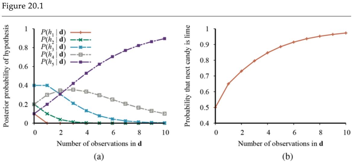
2 We stated earlier that the bags of candy are very large; otherwise, the i.i.d. assumption fails to hold. Technically, it is more correct (but less hygienic) to rewrap each candy after inspection and return it to the bag.

1. Posterior probabilities from Equation (20.1) . The number of observations ranges from 1 to 10, and each observation is of a lime candy. (b) Bayesian prediction from Equation (20.2) .

The example shows that the Bayesian prediction eventually agrees with the true hypothesis. This is characteristic of Bayesian learning. For any fixed prior that does not rule out the true hypothesis, the posterior probability of any false hypothesis will, under certain technical conditions, eventually vanish. This happens simply because the probability of generating “uncharacteristic” data indefinitely is vanishingly small. (This point is analogous to one made in the discussion of PAC learning in Chapter 19 .) More important, the Bayesian prediction is optimal, whether the data set is small or large. Given the hypothesis prior, any other prediction is expected to be correct less often.

The optimality of Bayesian learning comes at a price, of course. For real learning problems, the hypothesis space is usually very large or infinite, as we saw in Chapter 19 . In some cases, the summation in Equation (20.2) (or integration, in the continuous case) can be carried out tractably, but in most cases we must resort to approximate or simplified methods.

A very common approximation—one that is usually adopted in science—is to make predictions based on a single most probable hypothesis—that is, an that maximizes . This is often called a maximum a posteriori or MAP (pronounced “em-ay-pee”) hypothesis. Predictions made according to an MAP hypothesis are approximately Bayesian to the extent that . In our candy example, after three lime candies in a row, so the MAP learner then predicts that the fourth candy is lime with probability 1.0—a much more dangerous prediction than the Bayesian prediction of 0.8 shown in Figure 20.1(b) . As more data arrive, the MAP and Bayesian predictions become closer, because the competitors to the MAP hypothesis become less and less probable.

Maximum a posteriori

Although this example doesn’t show it, finding MAP hypotheses is often much easier than Bayesian learning, because it requires solving an optimization problem instead of a large summation (or integration) problem.

In both Bayesian learning and MAP learning, the hypothesis prior plays an important role. We saw in Chapter 19 that overfitting can occur when the hypothesis space is too expressive, that is, when it contains many hypotheses that fit the data set well. Bayesian and MAP learning methods use the prior to penalize complexity. Typically, more complex hypotheses have a lower prior probability—in part because there so many of them. On the other hand, more complex hypotheses have a greater capacity to fit the data. (In the extreme case, a lookup table can reproduce the data exactly.) Hence, the hypothesis prior embodies a tradeoff between the complexity of a hypothesis and its degree of fit to the data.

We can see the effect of this tradeoff most clearly in the logical case, where contains only deterministic hypotheses (such as , which says that every candy is cherry). In that case, is 1 if is consistent and 0 otherwise. Looking at Equation (20.1) , we see that will then be the simplest logical theory that is consistent with the data. Therefore, maximum a posteriori learning provides a natural embodiment of Ockham’s razor.

Another insight into the tradeoff between complexity and degree of fit is obtained by taking the logarithm of Equation (20.1) . Choosing to maximize is equivalent to minimizing

\[-\log\_2 P\left(\mathbf{d}|h\_i\right) - \log\_2 P\left(h\_i\right).\]

Using the connection between information encoding and probability that we introduced in Section 19.3.3 , we see that the term equals the number of bits required to specify the hypothesis . Furthermore, is the additional number of bits required to specify the data, given the hypothesis. (To see this, consider that no bits are required if the hypothesis predicts the data exactly—as with and the string of lime candies —and .) Hence, MAP learning is choosing the hypothesis that provides maximum compression of the data. The same task is addressed more directly by the minimum description length, or MDL, learning method. Whereas MAP learning expresses simplicity by assigning higher probabilities to simpler hypotheses, MDL expresses it directly by counting the bits in a binary encoding of the hypotheses and data.

A final simplification is provided by assuming a uniform prior over the space of hypotheses. In that case, MAP learning reduces to choosing an that maximizes . This is called a maximum-likelihood hypothesis, . Maximum-likelihood learning is very common in statistics, a discipline in which many researchers distrust the subjective nature of hypothesis

priors. It is a reasonable approach when there is no reason to prefer one hypothesis over another a priori—for example, when all hypotheses are equally complex.

Maximum-likelihood

When the data set is large, the prior distribution over hypotheses is less important—the evidence from the data is strong enough to swamp the prior distribution over hypotheses. That means maximum likelihood learning is a good approximation to Bayesian and MAP learning with large data sets, but it has problems (as we shall see) with small data sets.

20.2 Learning with Complete Data

The general task of learning a probability model, given data that are assumed to be generated from that model, is called density estimation. (The term applied originally to probability density functions for continuous variables, but it is used now for discrete distributions too.) Density estimation is a form of unsupervised learning. This section covers the simplest case, where we have complete data. Data are complete when each data point contains values for every variable in the probability model being learned. We focus on parameter learning—finding the numerical parameters for a probability model whose structure is fixed. For example, we might be interested in learning the conditional probabilities in a Bayesian network with a given structure. We will also look briefly at the problem of learning structure and at nonparametric density estimation.

Density estimation

Complete data

Parameter learning

20.2.1 Maximum-likelihood parameter learning: Discrete models

Suppose we buy a bag of lime and cherry candy from a new manufacturer whose flavor proportions are completely unknown; the fraction of cherry could be anywhere between 0 and 1. In that case, we have a continuum of hypotheses. The parameter in this case, which we call , is the proportion of cherry candies, and the hypothesis is . (The proportion of lime candies is just .) If we assume that all proportions are equally likely a priori, then a maximum-likelihood approach is reasonable. If we model the situation with a Bayesian network, we need just one random variable, (the flavor of a randomly chosen candy from the bag). It has values and , where the probability of is (see Figure 20.2(a) ). Now suppose we unwrap candies, of which are cherry and are lime. According to Equation (20.3) , the likelihood of this particular data set is

\[P\left(\mathbf{d} \middle| h\_{\theta}\right) = \prod\_{j=1}^{N} P\left(d\_{j} \middle| h\_{\theta}\right) = \theta^{c} \cdot \left(1 - \theta\right)^{\ell}.\]

The maximum-likelihood hypothesis is given by the value of that maximizes this expression. Because the function is monotonic, the same value is obtained by maximizing the log likelihood instead:

\[L\left(\mathbf{d}\Big|h\_{\theta}\right) = \log P\left(\mathbf{d}\Big|h\_{\theta}\right) = \sum\_{j=1}^{N} \log P\left(d\_{j}\Big|h\_{\theta}\right) = c\log\theta + \ell\log\left(1-\theta\right)\]

Log likelihood

(By taking logarithms, we reduce the product to a sum over the data, which is usually easier to maximize.) To find the maximum-likelihood value of , we differentiate with respect to and set the resulting expression to zero:

\[\frac{dL(\mathbf{d}|h\_{\theta})}{d\theta} = \frac{c}{\theta} - \frac{\ell}{1-\theta} = 0 \qquad \Rightarrow \qquad \theta = \frac{c}{c+\ell} = \frac{c}{N} \dots\]

In English, then, the maximum-likelihood hypothesis asserts that the actual proportion of cherry candies in the bag is equal to the observed proportion in the candies unwrapped so far!

It appears that we have done a lot of work to discover the obvious. In fact, though, we have laid out one standard method for maximum-likelihood parameter learning, a method with broad applicability:

• 1. Write down an expression for the likelihood of the data as a function of the parameter(s).
• 2. Write down the derivative of the log likelihood with respect to each parameter.
• 3. Find the parameter values such that the derivatives are zero.

The trickiest step is usually the last. In our example, it was trivial, but we will see that in many cases we need to resort to iterative solution algorithms or other numerical optimization techniques, as described in Section 4.2 . (We will need to verify that the Hessian matrix is negative-definite.) The example also illustrates a significant problem with maximum-likelihood learning in general: when the data set is small enough that some events have not yet been observed—for instance, no cherry candies—the maximum-likelihood hypothesis assigns zero probability to those events. Various tricks are used to avoid this problem, such as initializing the counts for each event to 1 instead of 0.

Let us look at another example. Suppose this new candy manufacturer wants to give a little hint to the consumer and uses candy wrappers colored red and green. The for each candy is selected probabilistically, according to some unknown conditional distribution, depending on the flavor. The corresponding probability model is shown in Figure 20.2(b) . Notice that it has three parameters: , , and . With these parameters, the likelihood of seeing, say, a cherry candy in a green wrapper can be obtained from the standard semantics for Bayesian networks (page 415):

\[\begin{aligned} &P\left(Flavor = charge, Wrapper = green|h\_{\theta,\theta\_1,\theta\_2}\right) \\ &= P\left(Flavor = charge |h\_{\theta,\theta\_1,\theta\_2}\right) P\left(Wrapper = green|Flavor = charge, h\_{\theta,\theta\_1,\theta\_2}\right) \\ &= \theta \cdot \left(1 - \theta\_1\right) .\end{aligned}\]

Figure 20.2

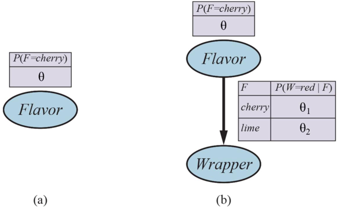
1. Bayesian network model for the case of candies with an unknown proportion of cherry and lime. (b) Model for the case where the wrapper color depends (probabilistically) on the candy flavor.

Now we unwrap candies, of which are cherry and are lime. The wrapper counts are as follows: of the cherry candies have red wrappers and have green, while of the lime candies have red and have green. The likelihood of the data is given by

\[P\left(\mathbf{d}\Big|h\_{\theta,\theta\_1,\theta\_2}\right) = \theta^c \left(1-\theta\right)^\ell \cdot \theta\_1^{r\_c} \left(1-\theta\_1\right)^{g\_c} \cdot \theta\_2^{r\_\ell} \left(1-\theta\_2\right)^{g\_\ell}.\]

This looks pretty horrible, but taking logarithms helps:

\[L = \left[c\log\theta + \ell\log(1-\theta)\right] + \left[r\_c\log\theta\_1 + g\_c\log(1-\theta\_1)\right] + \left[r\_\ell\log\theta\_2 + g\_\ell\log(1-\theta\_2)\right].\]

The benefit of taking logs is clear: the log likelihood is the sum of three terms, each of which contains a single parameter. When we take derivatives with respect to each parameter and set them to zero, we get three independent equations, each containing just one parameter:

\[\begin{aligned} \frac{\partial L}{\partial \theta} &=& \frac{c}{\theta} - \frac{\ell}{1 - \theta} = 0 & \Rightarrow & \theta = \frac{c}{c + \ell} \\ \frac{\partial L}{\partial \theta\_1} &=& \frac{r\_c}{\theta\_1} - \frac{g\_c}{1 - \theta\_1} = 0 & \Rightarrow & \theta\_1 = \frac{r\_c}{r\_c + g\_c} \\ \frac{\partial L}{\partial \theta\_2} &=& \frac{r\_\ell}{\theta\_2} - \frac{g\_\ell}{1 - \theta\_2} = 0 & \Rightarrow & \theta\_2 = \frac{r\_\ell}{r\_\ell + g\_\ell} \end{aligned}\]

The solution for is the same as before. The solution for , the probability that a cherry candy has a red wrapper, is the observed fraction of cherry candies with red wrappers, and similarly for .

These results are very comforting, and it is easy to see that they can be extended to any Bayesian network whose conditional probabilities are represented as tables. The most important point is that with complete data, the maximum-likelihood parameter learning problem for a Bayesian network decomposes into separate learning problems, one for each parameter. (See Exercise 20.NORX for the nontabulated case, where each parameter affects several conditional probabilities.) The second point is that the parameter values for a variable, given its parents, are just the observed frequencies of the variable values for each setting of the parent values. As before, we must be careful to avoid zeroes when the data set is small.

20.2.2 Naive Bayes models

Probably the most common Bayesian network model used in machine learning is the naive Bayes model first introduced on page 402. In this model, the “class” variable (which is to be predicted) is the root and the “attribute” variables are the leaves. The model is “naive” because it assumes that the attributes are conditionally independent of each other, given the class. (The model in Figure 20.2(b) is a naive Bayes model with class and just one attribute, Wrapper.) In the case of Boolean variables, the parameters are

\[ \theta = P(C = true), \\ \theta\_{i1} = P(X\_i = true | C = true), \\ \theta\_{i2} = P(X\_i = true | C = false). \]

The maximum-likelihood parameter values are found in exactly the same way as in Figure 20.2(b) . Once the model has been trained in this way, it can be used to classify new examples for which the class variable is unobserved. With observed attribute values , the probability of each class is given by

\[\mathbf{P}\left(C\middle|x\_1,\ldots,x\_n\right) = \alpha \cdot \mathbf{P}\left(C\right)\prod\_{i} \mathbf{P}\left(x\_i \middle| C\right)\dots\]

A deterministic prediction can be obtained by choosing the most likely class. Figure 20.3 shows the learning curve for this method when it is applied to the restaurant problem from Chapter 19 . The method learns fairly well but not as well as decision tree learning; this is presumably because the true hypothesis—which is a decision tree—is not representable exactly using a naive Bayes model. Naive Bayes learning turns out to do surprisingly well in a wide range of applications; the boosted version (Exercise 20.BNBX) is one of the most effective general-purpose learning algorithms. Naive Bayes learning scales well to very large problems: with Boolean attributes, there are just parameters, and no search is required to find , the maximum-likelihood naive Bayes hypothesis. Finally, naive Bayes learning systems deal well with noisy or missing data and can give probabilistic predictions when appropriate. Their primary drawback is the fact that the conditional independence assumption is seldom accurate; as noted on page 403, the assumption leads to overconfident probabilities that are often very close to 0 or 1, especially with large numbers of attributes.

Figure 20.3

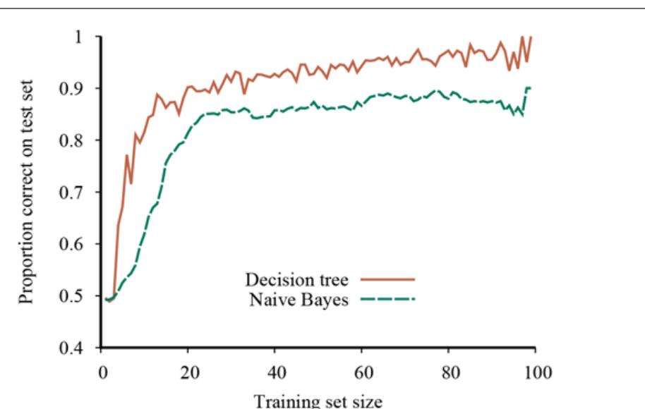
The learning curve for naive Bayes learning applied to the restaurant problem from Chapter 19 ; the learning curve for decision tree learning is shown for comparison.

20.2.3 Generative and discriminative models

We can distinguish two kinds of machine learning models used for classifiers: generative and discriminative. A generative model models the probability distribution of each class. For example, the naive Bayes text classifier from Section 12.6.1 creates a separate model for each possible category of text—one for sports, one for weather, and so on. Each model includes the prior probability of the category—for example —as well as the conditional probability . From these we can compute the joint probability and we can generate a random selection of words that is representative of texts in the weather category.

Generative model

A discriminative model directly learns the decision boundary between classes. That is, it learns . Given example inputs, a discriminative model will come up with an output category, but you cannot use a discriminative model to, say, generate random words that are representative of a category. Logistic regression, decision trees, and support vector machines are all discriminative models.

Discriminative model

Since discriminative models put all their emphasis on defining the decision boundary—that is, actually doing the classification task they were asked to do—they tend to perform better in the limit, with an arbitrary amount of training data. However, with limited data, in some cases a generative model performs better. (Ng and Jordan, 2002) compare the generative naive Bayes classifier to the discriminative logistic regression classifier on 15 (small) data sets, and find that with the maximum amount of data, the discriminative model does better on 9 out of 15 data sets, but with only a small amount of data, the generative model does better on 14 out of 15 data sets.

20.2.4 Maximum-likelihood parameter learning: Continuous models

Continuous probability models such as the linear–Gaussian model were shown on page 422. Because continuous variables are ubiquitous in real-world applications, it is important to know how to learn the parameters of continuous models from data. The principles for maximum-likelihood learning are identical in the continuous and discrete cases.

Let us begin with a very simple case: learning the parameters of a Gaussian density function on a single variable. That is, we assume the data are generated as follows:

\[P\left(x\right) = \frac{1}{\sigma\sqrt{2\pi}}e^{-\frac{\left(x-\mu\right)^2}{2\sigma^2}}.\]

The parameters of this model are the mean and the standard deviation . (Notice that the normalizing “constant” depends on , so we cannot ignore it.) Let the observed values be . Then the log likelihood is

\[L = \sum\_{j=1}^{N} \log \frac{1}{\sigma \sqrt{2\pi}} e^{-\frac{\binom{x\_{j-\mu}}{2\sigma^2}}{2\sigma^2}} = N \left( -\log \sqrt{2\pi} - \log \sigma \right) - \sum\_{j=1}^{N} \frac{\left( x\_j - \mu \right)^2}{2\sigma^2}.\]

Setting the derivatives to zero as usual, we obtain

(20.4)

\[\begin{array}{rclclcl}\frac{\partial L}{\partial \mu} &=& -\frac{1}{\sigma^2} \sum\_{j=1}^{N} \left( x\_j - \mu \right) = 0 & & \Rightarrow & \mu = \frac{\sum\_{j} x\_j}{N} \\\\ \frac{\partial L}{\partial \sigma} &=& -\frac{N}{\sigma} + \frac{1}{\sigma^3} \sum\_{j=1}^{N} \left( x\_j - \mu \right)^2 = 0 & & \Rightarrow & \sigma = \sqrt{\frac{\sum\_{j} \left( x\_j - \mu \right)^2}{N}} \end{array}\]

That is, the maximum-likelihood value of the mean is the sample average and the maximum-likelihood value of the standard deviation is the square root of the sample variance. Again, these are comforting results that confirm “commonsense” practice.

Now consider a linear–Gaussian model with one continuous parent and a continuous child . As explained on page 422, has a Gaussian distribution whose mean depends linearly on the value of and whose standard deviation is fixed. To learn the conditional distribution , we can maximize the conditional likelihood

\[P\left(y\middle|x\right) = \frac{1}{\sigma\sqrt{2\pi}}e^{-\frac{\left(\wp - \left(\mathfrak{s}\_{1^{\sigma + \mathfrak{s}\_2}}\right)\right)^2}{2\sigma^2}}.\]

Here, the parameters are , , and . The data are a collection of pairs, as illustrated in Figure 20.4 . Using the usual methods (Exercise 20.LINR), we can find the maximum-likelihood values of the parameters. The point here is different. If we consider just the parameters and that define the linear relationship between and , it becomes clear that maximizing the log likelihood with respect to these parameters is the same as minimizing the numerator in the exponent of Equation (20.5) . This is the loss, the squared error between the actual value and the prediction .

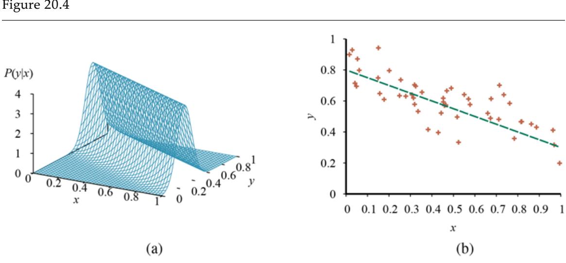
1. A linear–Gaussian model described as plus Gaussian noise with fixed variance. (b) A set of 50 data points generated from this model and the best-fit line.

This is the quantity minimized by the standard linear regression procedure described in Section 19.6 . Now we can understand why: minimizing the sum of squared errors gives the maximum-likelihood straight-line model, provided that the data are generated with Gaussian noise of fixed variance.

20.2.5 Bayesian parameter learning

Maximum-likelihood learning gives rise to simple procedures, but it has serious deficiencies with small data sets. For example, after seeing one cherry candy, the maximum-likelihood hypothesis is that the bag is 100% cherry (i.e., ). Unless one’s hypothesis prior is that

bags must be either all cherry or all lime, this is not a reasonable conclusion. It is more likely that the bag is a mixture of lime and cherry. The Bayesian approach to parameter learning starts with a hypothesis prior and updates the distribution as data arrive.

The candy example in Figure 20.2(a) has one parameter, : the probability that a randomly selected piece of candy is cherry-flavored. In the Bayesian view, is the (unknown) value of a random variable that defines the hypothesis space; the hypothesis prior is the prior distribution over . Thus, is the prior probability that the bag has a fraction of cherry candies.

If the parameter can be any value between 0 and 1, then is a continuous probability density function (see Section A.3 ). If we don’t know anything about the possible values of we can use the uniform density function , which says all values are equally likely.

A more flexible family of probability density functions is known as the beta distributions. Each beta distribution is defined by two hyperparameters and such that 3

(20.6)

\[ \operatorname{Beta} \left( \theta; a, b \right) = \alpha \; \theta^{a-1} \left( 1 - \theta \right)^{b-1}, \]

3 They are called hyperparameters because they parameterize a distribution over , which is itself a parameter.

Beta distribution

Hyperparameter

for in the range . The normalization constant , which makes the distribution integrate to 1, depends on and . Figure 20.5 shows what the distribution looks like for various values of and . The mean value of the beta distribution is , so larger values of suggest a belief that is closer to 1 than to 0. Larger values of make the distribution more peaked, suggesting greater certainty about the value of . It turns out that the uniform density function is the same as : the mean is , and the distribution is flat.

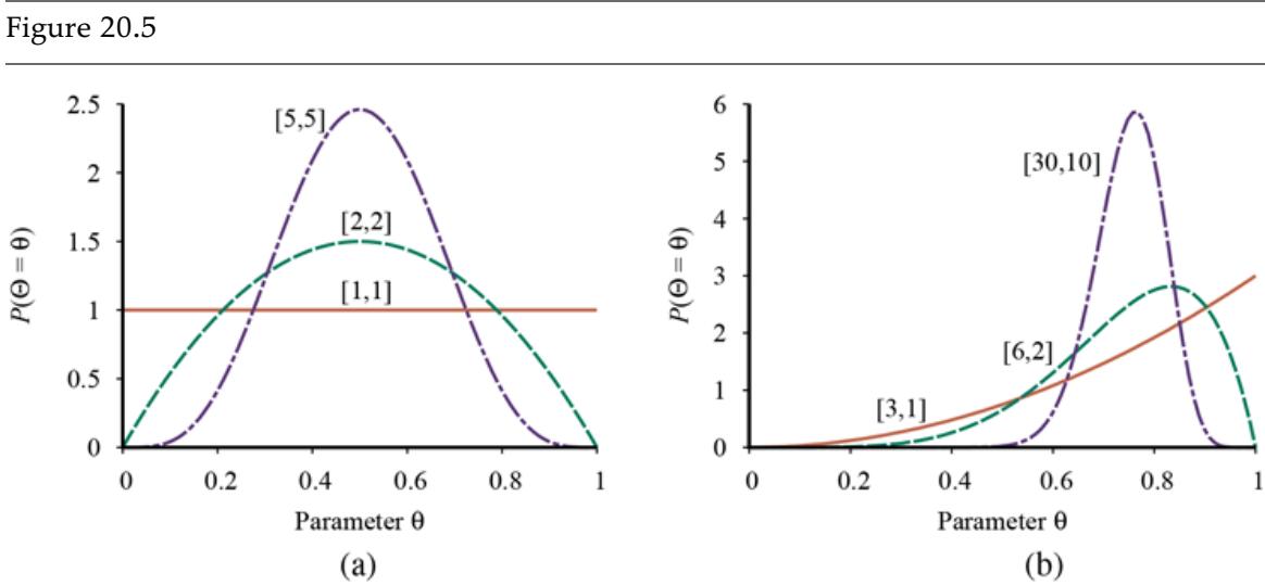
Examples of the distribution for different values of .

Besides its flexibility, the beta family has another wonderful property: if has a prior , then, after a data point is observed, the posterior distribution for is also a beta distribution. In other words, is closed under update. The beta family is called the conjugate prior for the family of distributions for a Boolean variable. Let’s see how this works. Suppose we observe a cherry candy; then we have 4

4 Other conjugate priors include the Dirichlet family for the parameters of a discrete multivalued distribution and the Normal– Wishart family for the parameters of a Gaussian distribution. See Bernardo and Smith (1994).

\[\begin{aligned} P(\theta|D\_1 = \text{cherr} y) &= \alpha \, P(D\_1 = \text{cherr} y | \theta) P(\theta) \\ &= \alpha' \, \theta \cdot \text{Beta} \left(\theta; a, b\right) = \alpha' \, \theta \cdot \theta^{a-1} \left(1 - \theta\right)^{b-1} \\ &= \alpha' \, \theta^a \left(1 - \theta\right)^{b-1} = \alpha' \, \text{Beta} \left(\theta; a + 1, b\right). \end{aligned}\]

Conjugate prior

Thus, after seeing a cherry candy, we simply increment the parameter to get the posterior; similarly, after seeing a lime candy, we increment the parameter. Thus, we can view the and hyperparameters as virtual counts, in the sense that a prior behaves exactly as if we had started out with a uniform prior and seen actual cherry candies and actual lime candies.

Virtual count

By examining a sequence of beta distributions for increasing values of and , keeping the proportions fixed, we can see vividly how the posterior distribution over the parameter changes as data arrive. For example, suppose the actual bag of candy is 75% cherry. Figure 20.5(b) shows the sequence , , . Clearly, the distribution is converging to a narrow peak around the true value of . For large data sets, then, Bayesian learning (at least in this case) converges to the same answer as maximum-likelihood learning.

Now let us consider a more complicated case. The network in Figure 20.2(b) has three parameters, , , and , where is the probability of a red wrapper on a cherry candy and is the probability of a red wrapper on a lime candy. The Bayesian hypothesis prior must cover all three parameters—that is, we need to specify . Usually, we assume parameter independence:

\[\mathbf{P}(\Theta, \Theta\_1, \Theta\_2) = \mathbf{P}(\Theta)\mathbf{P}(\Theta\_1)\mathbf{P}(\Theta\_2)\dots\]

Parameter independence

With this assumption, each parameter can have its own beta distribution that is updated separately as data arrive. Figure 20.6 shows how we can incorporate the hypothesis prior and any data into a Bayesian network, in which we have a node for each parameter variable.

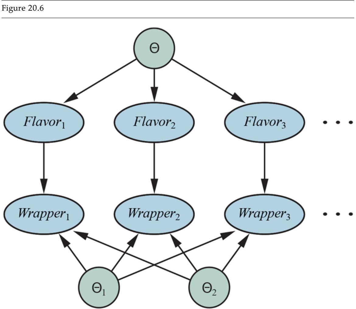
A Bayesian network that corresponds to a Bayesian learning process. Posterior distributions for the parameter variables , , and can be inferred from their prior distributions and the evidence in and .

The nodes have no parents. For the th observation of a wrapper and corresponding flavor of a piece of candy, we add nodes and . is dependent on the flavor parameter :

\[P(Flavar\_i = herry| Θ = θ) = θ ...\]

is dependent on and :

Now, the entire Bayesian learning process for the original Bayes net in Figure 20.2(b) can be formulated as an inference problem in the derived Bayes net shown in Figure 20.6 , where the data and parameters become nodes. Once we have added all the new evidence nodes, we can then query the parameter variables (in this case, ). Under this formulation there is just one learning algorithm—the inference algorithm for Bayesian networks.

Of course, the nature of these networks is somewhat different from those of Chapter 13 because of the potentially huge number of evidence variables representing the training set and the prevalence of continuous-valued parameter variables. Exact inference may be impossible except in very simple cases such as the naive Bayes model. Practitioners typically use approximate inference methods such as MCMC (Section 13.4.2 ); many statistical software packages incorporate efficient implementations of MCMC for this purpose.

20.2.6 Bayesian linear regression

Here we illustrate how to apply a Bayesian approach to a standard statistical task: linear regression. The conventional approach was described in Section 19.6 as minimizing the sum of squared errors and reinterpreted in Section 20.2.4 as maximizing likelihood assuming a Gaussian error model. These produce a single best hypothesis: a straight line with specific values for the slope and intercept and a fixed variance for the prediction error at any given point. There is no measure of how confident one should be in the slope and intercept values.

Furthermore, if one is predicting a value for an unseen data point far from the observed data points, it seems to make no sense to assume a prediction error that is the same as the prediction error for a data point right next to an observed data point. It would seem more sensible for the prediction error to be larger, the farther the data point is from the observed data, because a small change in the slope will cause a large change in the predicted value for a distant point.

The Bayesian approach fixes both of these problems. The general idea, as in the preceding section, is to place a prior on the model parameters—here, the coefficients of the linear

model and the noise variance—and then to compute the parameter posterior given the data. For multivariate data and unknown noise model, this leads to rather a lot of linear algebra, so we focus on a simple case: univariable data, a model that is constrained to go through the origin, and known noise: a normal distribution with variance . Then we have just one parameter and the model is

(20.7)

\[P\left(y|x,\theta\right) = N\left(y;\theta x,\sigma\_y^2\right) = \frac{1}{\sigma\sqrt{2\pi}}e^{-\frac{1}{2}\left(\frac{\left(y-\theta x\right)^2}{\sigma^2}\right)}\]

As the log likelihood is quadratic in , the appropriate form for a conjugate prior on is also a Gaussian. This ensures that the posterior for will also be Gaussian. We’ll assume a mean and variance for the prior, so that

(20.8)

\[P\left(\theta \atop \theta \right) = N\left(\theta; \theta\_0, \sigma\_0^2\right) = \frac{1}{\sigma\_0 \sqrt{2\pi}} e^{-\frac{1}{2} \left(\frac{\left(\theta - \theta\_0\right)^2}{\sigma\_0^2}\right)}\]

Uninformative prior

Depending on the data being modeled, one might have some idea of what sort of slope to expect, or one might be completely agnostic. In the latter case, it makes sense to choose to be 0 and to be large—a so-called uninformative prior. Finally, we can assume a prior for the -value of each data point, but this is completely immaterial to the analysis because it doesn’t depend on .

Now the setup is complete, so we can compute the posterior for using Equation (20.1) : . The observed data points are , so the

likelihood for the data is obtained from Equation (20.7) as follows:

\[\begin{aligned} P(\mathbf{d}|\boldsymbol{\theta}) &= \left(\prod\_{i} P(x\_i)\right) \prod\_{i} P(y\_i|x\_i, \boldsymbol{\theta}) = \alpha \prod\_{i} e^{-\frac{1}{2} \left(\frac{(y\_i - \theta x\_i)^2}{\sigma^2}\right)} \\ &= \alpha e^{-\frac{1}{2} \sum\_{i} \left(\frac{(y\_i - \theta x\_i)^2}{\sigma^2}\right)}, \end{aligned}\]

where we have absorbed the -value priors and the normalizing constants for the Gaussians into a constant that is independent of . Now we combine this and the parameter prior from Equation (20.8) to obtain the posterior:

\[P\left(\theta \middle| \mathbf{d} \right) = \alpha'' e^{-\frac{1}{2} \left( \frac{\left(\theta - \theta\_0\right)^2}{\sigma\_0^2} \right)} e^{-\frac{1}{2} \sum\_i \left( \frac{\left(\chi\_i - \theta x\_i\right)^2}{\sigma^2} \right)}\]

Although this looks complicated, each exponent is a quadratic function of , so the sum of the two exponents is as well. Hence, the whole expression represents a Gaussian distribution for . Using algebraic manipulations very similar to those in Section 14.4 , we find

\[P\left(\boldsymbol{\theta} \middle| \mathbf{d} \middle| \begin{array}{c} \\ \boldsymbol{\theta} \middle| \mathbf{d} \\ \boldsymbol{\theta} \\ \hline \end{array} \right) = \boldsymbol{\alpha}^{\prime\prime\prime} \boldsymbol{e}^{-\frac{1}{2} \left( \frac{\left(\boldsymbol{\theta} - \boldsymbol{\theta}\_{N}\right)^{2}}{\sigma\_{N}^{2}} \right)}\]

with “updated” mean and variance given by

\[\theta\_N = \frac{\sigma^2 \theta\_0 + \sigma\_0^2 \sum\_i x\_i y\_i}{\sigma^2 + \sigma\_0^2 \sum\_i x\_i^2} \quad \text{and} \quad \sigma\_N^2 = \frac{\sigma^2 \sigma\_0^2}{\sigma^2 + \sigma\_0^2 \sum\_i x\_i^2}.\]

Let’s look at these formulas to see what they mean. When the data are narrowly concentrated on a small region of the -axis near the origin, will be small and the posterior variance will be large, roughly equal to the prior variance . This is as one would expect: the data do little to constrain the rotation of the line around the origin. Conversely, when the data are widely spread along the axis, will be large and the

posterior variance will be small, roughly equal to , so the slope will be very tightly constrained.

To make a prediction at a specific data point, we have to integrate over the possible values of , as suggested by Equation (20.2) :

\[\begin{split} P(y|x,\mathbf{d}) &= \int\_{-\infty}^{\infty} P(y|x,\mathbf{d},\theta)P(\theta|x,\mathbf{d})d\theta = \int\_{-\infty}^{\infty} P(y|x,\theta)P(\theta|\mathbf{d})d\theta \\ &= \quad \alpha \int\_{-\infty}^{\infty} e^{-\frac{1}{2}\left(\frac{(y-\theta x)^{2}}{\sigma^{2}}\right)} e^{-\frac{1}{2}\left(\frac{(\theta-\theta\_{N})^{2}}{\sigma^{2}\_{N}}\right)} d\theta \end{split}\]

Again, the sum of the two exponents is a quadratic function of , so we have a Gaussian over whose integral is 1. The remaining terms in form another Gaussian:

\[P\left(y \middle| x, \mathbf{d}\right) \propto e^{-\frac{1}{2}\left(\frac{\left(y - \theta\_N \overline{\ast}\right)^2}{\sigma^2 + \sigma\_N^2 x^2}\right)}\]

Looking at this expression, we see that the mean prediction for is , that is, it is based on the posterior mean for . The variance of the prediction is given by the model noise plus a term proportional to , which means that the standard deviation of the prediction increases asymptotically linearly with the distance from the origin. Figure 20.7 illustrates this phenomenon. As noted at the beginning of this section, having greater uncertainty for predictions that are further from the observed data points makes perfect sense.

Figure 20.7

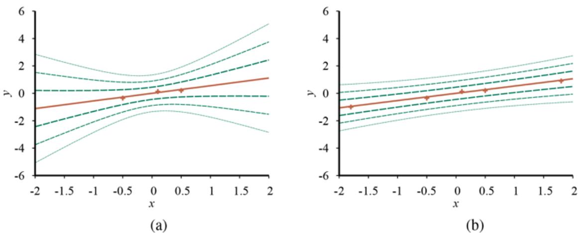
Bayesian linear regression with a model constrained to pass through the origin and fixed noise variance . Contours at , , and standard deviations are shown for the predictive density. (a) With three data points near the origin, the slope is quite uncertain, with . Notice how the uncertainty increases with distance from the observed data points. (b) With two additional data points further away, the slope is very tightly constrained, with . The remaining variance in the predictive density is almost entirely due to the fixed noise .

20.2.7 Learning Bayes net structures

So far, we have assumed that the structure of the Bayes net is given and we are just trying to learn the parameters. The structure of the network represents basic causal knowledge about the domain that is often easy for an expert, or even a naive user, to supply. In some cases, however, the causal model may be unavailable or subject to dispute—for example, certain corporations have long claimed that smoking does not cause cancer and other corporations assert that concentrations have no effect on climate—so it is important to understand how the structure of a Bayes net can be learned from data. This section gives a brief sketch of the main ideas.

The most obvious approach is to search for a good model. We can start with a model containing no links and begin adding parents for each node, fitting the parameters with the methods we have just covered and measuring the accuracy of the resulting model. Alternatively, we can start with an initial guess at the structure and use hill climbing or simulated annealing search to make modifications, retuning the parameters after each change in the structure. Modifications can include reversing, adding, or deleting links. We must not introduce cycles in the process, so many algorithms assume that an ordering is given for the variables, and that a node can have parents only among those nodes that come earlier in the ordering (just as in the construction process in Chapter 13 ). For full generality, we also need to search over possible orderings.

There are two alternative methods for deciding when a good structure has been found. The first is to test whether the conditional independence assertions implicit in the structure are actually satisfied in the data. For example, the use of a naive Bayes model for the restaurant problem assumes that

and we can check in the data whether the same equation holds between the corresponding conditional frequencies. But even if the structure describes the true causal nature of the domain, statistical fluctuations in the data set mean that the equation will never be satisfied exactly, so we need to perform a suitable statistical test to see if there is sufficient evidence that the independence hypothesis is violated. The complexity of the resulting network will depend on the threshold used for this test—the stricter the independence test, the more links will be added and the greater the danger of overfitting.

An approach more consistent with the ideas in this chapter is to assess the degree to which the proposed model explains the data (in a probabilistic sense). We must be careful how we measure this, however. If we just try to find the maximum-likelihood hypothesis, we will end up with a fully connected network, because adding more parents to a node cannot decrease the likelihood (Exercise 20.MLPA). We are forced to penalize model complexity in some way. The MAP (or MDL) approach simply subtracts a penalty from the likelihood of each structure (after parameter tuning) before comparing different structures. The Bayesian approach places a joint prior over structures and parameters. There are usually far too many structures to sum over (superexponential in the number of variables), so most practitioners use MCMC to sample over structures.

Penalizing complexity (whether by MAP or Bayesian methods) introduces an important connection between the optimal structure and the nature of the representation for the conditional distributions in the network. With tabular distributions, the complexity penalty for a node’s distribution grows exponentially with the number of parents, but with, say, noisy-OR distributions, it grows only linearly. This means that learning with noisy-OR (or other compactly parameterized) models tends to produce learned structures with more parents than does learning with tabular distributions.

20.2.8 Density estimation with nonparametric models

It is possible to learn a probability model without making any assumptions about its structure and parameterization by adopting the nonparametric methods of Section 19.7 . The task of nonparametric density estimation is typically done in continuous domains, such as that shown in Figure 20.8(a) . The figure shows a probability density function on a space defined by two continuous variables. In Figure 20.8(b) we see a sample of data points from this density function. The question is, can we recover the model from the samples?

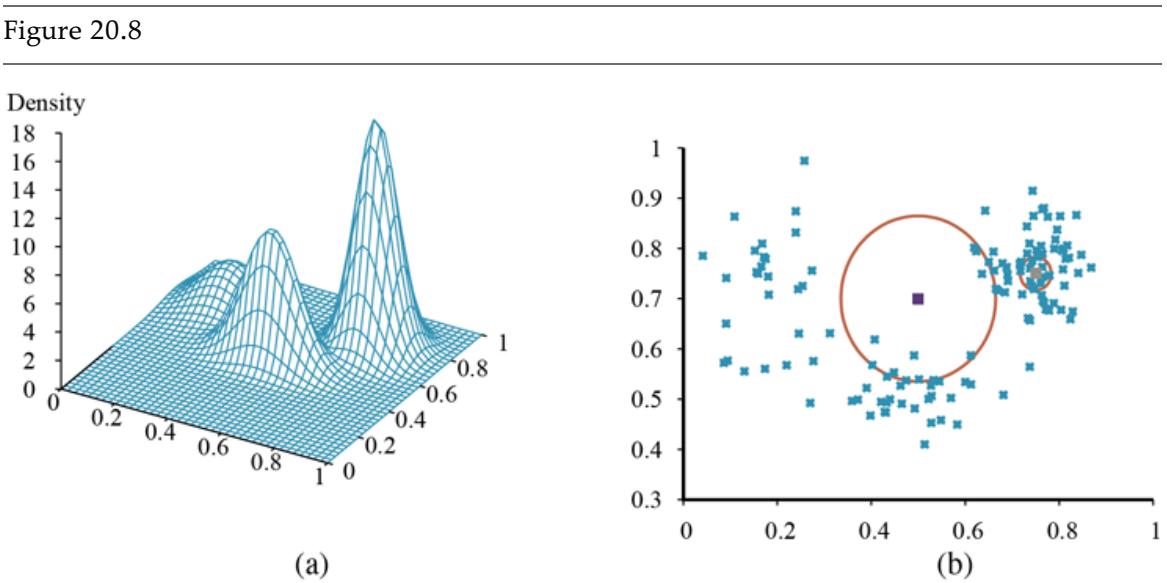
1. A 3D plot of the mixture of Gaussians from Figure 20.12(a) . (b) A 128-point sample of points from the mixture, together with two query points (small orange squares) and their -nearest-neighborhoods (large circle and smaller circle to the right).

Nonparametric density estimation

First we will consider -nearest-neighbors models. (In Chapter 19 we saw nearestneighbor models for classification and regression; here we see them for density estimation.) Given a sample of data points, to estimate the unknown probability density at a query point we can simply measure the density of the data points in the neighborhood of . Figure 20.8(b) shows two query points (small squares). For each query point we have drawn the smallest circle that encloses 10 neighbors—the 10-nearest-neighborhood. We can see that the central circle is large, meaning there is a low density there, and the circle on the right is

small, meaning there is a high density there. In Figure 20.9 we show three plots of density estimation using -nearest-neighbors, for different values of . It seems clear that (b) is about right, while (a) is too spiky ( is too small) and (c) is too smooth ( is too big).

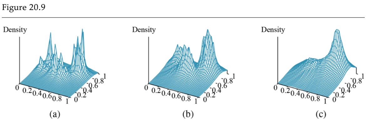
Density estimation using -nearest-neighbors, applied to the data in Figure 20.8(b) , for , , and respectively. is too spiky, 40 is too smooth, and 10 is just about right. The best value for can be chosen by cross-validation.

Another possibility is to use kernel functions, as we did for locally weighted regression. To apply a kernel model to density estimation, assume that each data point generates its own little density function. For example, we might use spherical Gaussians with standard deviation along each axis. Then estimated density at a query point is the average of the data kernels:

\[P\left(\mathbf{x}\right) = \frac{1}{N} \sum\_{j=1}^{N} K\left(\mathbf{x}, \mathbf{x}\_{j}\right) \quad \text{where} \quad K\left(\mathbf{x}, \mathbf{x}\_{j}\right) = \frac{1}{\left(w^{2}\sqrt{2\pi}\right)^{d}} e^{-\frac{\rho\left(\mathbf{x}, \mathbf{x}\_{j}\right)^{2}}{2\theta^{2}}},\]

where is the number of dimensions in and is the Euclidean distance function. We still have the problem of choosing a suitable value for kernel width ; Figure 20.10 shows values that are too small, just right, and too large. A good value of can be chosen by using cross-validation.

Figure 20.10

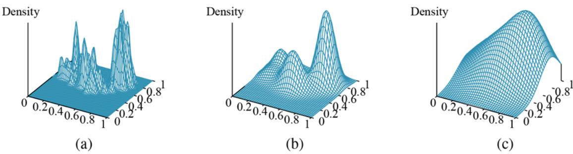
Density estimation using kernels for the data in Figure 20.8(b) , using Gaussian kernels with , , and respectively. is about right.

20.3 Learning with Hidden Variables: The EM Algorithm

Latent variable

The preceding section dealt with the fully observable case. Many real-world problems have hidden variables (sometimes called latent variables), which are not observable in the data. For example, medical records often include the observed symptoms, the physician’s diagnosis, the treatment applied, and perhaps the outcome of the treatment, but they seldom contain a direct observation of the disease itself! (Note that the diagnosis is not the disease; it is a causal consequence of the observed symptoms, which are in turn caused by the disease.) One might ask, “If the disease is not observed, could we construct a model based only on the observed variables?” The answer appears in Figure 20.11 , which shows a small, fictitious diagnostic model for heart disease. There are three observable predisposing factors and three observable symptoms (which are too depressing to name). Assume that each variable has three possible values (e.g., , , and ). Removing the hidden variable from the network in (a) yields the network in (b); the total number of parameters increases from 78 to 708. Thus, latent variables can dramatically reduce the number of parameters required to specify a Bayesian network. This, in turn, can dramatically reduce the amount of data needed to learn the parameters.

Figure 20.11

1. A simple diagnostic network for heart disease, which is assumed to be a hidden variable. Each variable has three possible values and is labeled with the number of independent parameters in its conditional distribution; the total number is 78. (b) The equivalent network with removed. Note that the symptom variables are no longer conditionally independent given their parents. This network requires 708 parameters.

Hidden variables are important, but they do complicate the learning problem. In Figure 20.11(a) , for example, it is not obvious how to learn the conditional distribution for , given its parents, because we do not know the value of in each case; the same problem arises in learning the distributions for the symptoms. This section describes an algorithm called expectation–maximization, or EM, that solves this problem in a very general way. We will show three examples and then provide a general description. The algorithm seems like magic at first, but once the intuition has been developed, one can find applications for EM in a huge range of learning problems.

Expectation–maximization

20.3.1 Unsupervised clustering: Learning mixtures of Gaussians

Unsupervised clustering is the problem of discerning multiple categories in a collection of objects. The problem is unsupervised because the category labels are not given. For example, suppose we record the spectra of a hundred thousand stars; are there different types of stars revealed by the spectra, and, if so, how many types and what are their characteristics? We are all familiar with terms such as “red giant” and “white dwarf,” but the stars do not carry these labels on their hats—astronomers had to perform unsupervised clustering to identify these categories. Other examples include the identification of species, genera, orders, phylum, and so on in the Linnaean taxonomy and the creation of natural kinds for ordinary objects (see Chapter 10 ).

Unsupervised clustering

Unsupervised clustering begins with data. Figure 20.12(b) shows 500 data points, each of which specifies the values of two continuous attributes. The data points might correspond to stars, and the attributes might correspond to spectral intensities at two particular frequencies. Next, we need to understand what kind of probability distribution might have generated the data. Clustering presumes that the data are generated from a mixture distribution, . Such a distribution has components, each of which is a distribution in its own right. A data point is generated by first choosing a component and then generating a sample from that component. Let the random variable denote the component, with values ; then the mixture distribution is given by

\[P\left(\mathbf{x}\right) = \sum\_{i=1}^{k} P\left(C = i\right) P\left(\mathbf{x} \middle| C = i\right),\]

Mixture distribution

Component

where refers to the values of the attributes for a data point. For continuous data, a natural choice for the component distributions is the multivariate Gaussian, which gives the socalled mixture of Gaussians family of distributions. The parameters of a mixture of

Gaussians are (the weight of each component), (the mean of each component), and (the covariance of each component). Figure 20.12(a) shows a mixture of three Gaussians; this mixture is in fact the source of the data in (b) as well as being the model shown in Figure 20.8(a) on page 736.

1. A Gaussian mixture model with three components; the weights (left-to-right) are 0.2, 0.3, and 0.5. (b) 500 data points sampled from the model in (a). (c) The model reconstructed by EM from the data in (b).

The unsupervised clustering problem, then, is to recover a Gaussian mixture model like the one in Figure 20.12(a) from raw data like that in Figure 20.12(b) . Clearly, if we knew which component generated each data point, then it would be easy to recover the component Gaussians: we could just select all the data points from a given component and then apply (a multivariate version of) Equation (20.4) (page 729) for fitting the parameters of a Gaussian to a set of data. On the other hand, if we knew the parameters of each component, then we could, at least in a probabilistic sense, assign each data point to a component.

The problem is that we know neither the assignments nor the parameters. The basic idea of EM in this context is to pretend that we know the parameters of the model and then to infer the probability that each data point belongs to each component. After that, we refit the components to the data, where each component is fitted to the entire data set with each point weighted by the probability that it belongs to that component. The process iterates until convergence. Essentially, we are “completing” the data by inferring probability distributions over the hidden variables—which component each data point belongs tobased on the current model. For the mixture of Gaussians, we initialize the mixture-model parameters arbitrarily and then iterate the following two steps:

• 1. E-STEP: Compute the probabilities , the probability that datum was generated by component . By Bayes’ rule, we have . The term is just the probability at of the th Gaussian, and the term is just the weight parameter for the th Gaussian. Define , the effective number of data points currently assigned to component .
• 2. M-STEP: Compute the new mean, covariance, and component weights using the following steps in sequence:

\[\begin{aligned} \mu\_i &\leftarrow \sum\_j p\_{ij} \mathbf{x}\_j / n\_i \\ \Sigma\_i &\leftarrow \sum\_j p\_{ij} \left(\mathbf{x}\_j - \mu\_i\right) \left(\mathbf{x}\_j - \mu\_i\right)^\top / n\_i \\ w\_i &\leftarrow n\_i / N \end{aligned}\]

where is the total number of data points. The E-step, or expectation step, can be viewed as computing the expected values of the hidden indicator variables , where is 1 if datum was generated by the th component and 0 otherwise. The M-step, or maximization step, finds the new values of the parameters that maximize the log likelihood of the data, given the expected values of the hidden indicator variables.

Indicator variable

The final model that EM learns when it is applied to the data in Figure 20.12(a) is shown in Figure 20.12(c) ; it is virtually indistinguishable from the original model from which the data were generated (horizontal line). Figure 20.13(a) plots the log likelihood of the data according to the current model as EM progresses.

Figure 20.13

Graphs showing the log likelihood of the data, , as a function of the EM iteration. The horizontal line shows the log likelihood according to the true model. (a) Graph for the Gaussian mixture model in Figure 20.12 . (b) Graph for the Bayesian network in Figure 20.14(a) .

There are two points to notice. First, the log likelihood for the final learned model slightly exceeds that of the original model, from which the data were generated. This might seem surprising, but it simply reflects the fact that the data were generated randomly and might not provide an exact reflection of the underlying model. The second point is that EM increases the log likelihood of the data at every iteration. This fact can be proved in general. Furthermore, under certain conditions (that hold in most cases), EM can be proven to reach a local maximum in likelihood. (In rare cases, it could reach a saddle point or even a local minimum.) In this sense, EM resembles a gradient-based hill-climbing algorithm, but notice that it has no “step size” parameter.

Things do not always go as well as Figure 20.13(a) might suggest. It can happen, for example, that one Gaussian component shrinks so that it covers just a single data point. Then its variance will go to zero and its likelihood will go to infinity! If we don’t know how many components are in the mixture we have to try different values of and see which is best; that can be a source of error. Another problem is that two components can “merge,” acquiring identical means and variances and sharing their data points. These kinds of degenerate local maxima are serious problems, especially in high dimensions. One solution is to place priors on the model parameters and to apply the MAP version of EM. Another is to restart a component with new random parameters if it gets too small or too close to another component. Sensible initialization also helps.

20.3.2 Learning Bayes net parameter values for hidden variables

To learn a Bayesian network with hidden variables, we apply the same insights that worked for mixtures of Gaussians. Figure 20.14(a) represents a situation in which there are two bags of candy that have been mixed together. Candies are described by three features: in addition to the and the , some candies have a in the middle and some do not. The distribution of candies in each bag is described by a naive Bayes model: the features are independent, given the bag, but the conditional probability distribution for each feature depends on the bag. The parameters are as follows: is the prior probability that a candy comes from Bag 1; and are the probabilities that the flavor is cherry, given that the candy comes from Bag 1 or Bag 2 respectively; and give the probabilities that the wrapper is red; and and give the probabilities that the candy has a hole.

The overall model is a mixture model: a weighted sum of two different distributions, each of which is a product of independent, univariate distributions. (In fact, we can also model the mixture of Gaussians as a Bayesian network, as shown in Figure 20.14(b) .) In the figure, the bag is a hidden variable because, once the candies have been mixed together, we no longer know which bag each candy came from. In such a case, can we recover the descriptions of the two bags by observing candies from the mixture? Let us work through an iteration of EM for this problem. First, let’s look at the data. We generated 1000 samples from a model whose true parameters are as follows:

(20.9)

\[ \theta = 0.5, \quad \theta\_{F1} = \theta\_{W1} = \theta\_{H1} = 0.8, \quad \theta\_{F2} = \theta\_{W2} = \theta\_{H2} = 0.3. \]

That is, the candies are equally likely to come from either bag; the first is mostly cherry with red wrappers and holes; the second is mostly lime with green wrappers and no holes. The counts for the eight possible kinds of candy are as follows:

		W = red	W = green
		H=1 H=0 H=1 H=0
=cherry F	273	93	104	90
F =lime	79	100	94	167

We start by initializing the parameters. For numerical simplicity, we arbitrarily choose 5

5 It is better in practice to choose them randomly, to avoid local maxima due to symmetry.

(20.10)

\[ \theta^{(0)} = 0.6, \ \theta\_{F1}^{(0)} = \theta\_{W1}^{(0)} = \theta\_{H1}^{(0)} = 0.6, \ \theta\_{F2}^{(0)} = \theta\_{W2}^{(0)} = \theta\_{H2}^{(0)} = 0.4 \ \dots \]

First, let us work on the parameter. In the fully observable case, we would estimate this directly from the observed counts of candies from bags 1 and 2. Because the bag is a hidden variable, we calculate the expected counts instead. The expected count is the sum, over all candies, of the probability that the candy came from bag 1:

\[\theta^{(1)} = \hat{N}\left(Bag = 1\right) / N = \sum\_{j=1}^{N} P\left(Bag = 1 \middle|{\ flavor\_j, wrapper\_j, holes\_j}\right) / N \ .\]

These probabilities can be computed by any inference algorithm for Bayesian networks. For a naive Bayes model such as the one in our example, we can do the inference “by hand,” using Bayes’ rule and applying conditional independence:

\[\theta^{\{1\}} = \frac{1}{N} \sum\_{j=1}^{N} \frac{P(f\_{\textit{f}}|\textit{Bag}=1)P(\textit{wapper}|\textit{Bag}=1)P(\textit{holes}|\textit{Bag}=1)P(\textit{Bag}=1)}{\sum\_{i}P(f\_{\textit{f}}|\textit{Bag}=i)P(\textit{wapper}\_{j}|\textit{Bag}=i)} \frac{P(\textit{boles}|\textit{Bag}=1)}{P(\textit{boles}|\textit{Bag}=i)P(\textit{Bag}=i)} \frac{1}{P(\textit{bage}=1)}\]

Applying this formula to, say, the 273 red-wrapped cherry candies with holes, we get a contribution of

\[\frac{273}{1000} \cdot \frac{\theta\_{F1}^{(0)}\theta\_{W1}^{(0)}\theta\_{H1}^{(0)}\theta^{(0)}}{\theta\_{F1}^{(0)}\theta\_{W1}^{(0)}\theta\_{H1}^{(0)}\theta^{(0)} + \theta\_{F2}^{(0)}\theta\_{W2}^{(0)}\theta\_{H2}^{(0)}\left(1-\theta^{(0)}\right)} \approx 0.22797\dots\]

Continuing with the other seven kinds of candy in the table of counts, we obtain .

Now let us consider the other parameters, such as . In the fully observable case, we would estimate this directly from the observed counts of cherry and lime candies from bag 1. The expected count of cherry candies from bag 1 is given by

\[\sum\_{j: Flavor\_j = chory} P(Bag = 1 | Flavor\_j = chory, wrapper\_j, holes\_j)\]

Again, these probabilities can be calculated by any Bayes net algorithm. Completing this process, we obtain the new values of all the parameters:

(20.11)

\[\begin{aligned} \theta^{(1)} &= 0.6124, \; \theta\_{F1}^{(1)} = 0.6684, \quad \theta\_{W1}^{(1)} = 0.6483, \; \theta\_{H1}^{(1)} = 0.6558, \\\ \theta\_{F2}^{(1)} &= 0.3887, \; \theta\_{W2}^{(1)} = 0.3817, \; \theta\_{H2}^{(1)} = 0.3827. \end{aligned}\]

The log likelihood of the data increases from about initially to about after the first iteration, as shown in Figure 20.13(b) . That is, the update improves the likelihood itself by a factor of about . By the tenth iteration, the learned model is a better fit than the original model ( ). Thereafter, progress becomes very slow. This is not uncommon with EM, and many practical systems combine EM with a gradient-based algorithm such as Newton–Raphson (see Chapter 4 ) for the last phase of learning.

The general lesson from this example is that the parameter updates for Bayesian network learning with hidden variables are directly available from the results of inference on each example. Moreover, only local posterior probabilities are needed for each parameter. Here, “local” means

that the conditional probability table (CPT) for each variable can be learned from posterior probabilities involving just and its parents . Defining to be the CPT parameter , the update is given by the normalized expected counts as follows:

\[\theta\_{ijk} \leftarrow \hat{N}\left(X\_i = x\_{ij}, \mathbf{U}\_i = \mathbf{u}\_{ik}\right) / \hat{N}\left(\mathbf{U}\_i = \mathbf{u}\_{ik}\right).\]

The expected counts are obtained by summing over the examples, computing the probabilities for each by using any Bayes net inference algorithm. For the exact algorithms—including variable elimination—all these probabilities are obtainable directly as a by-product of standard inference, with no need for extra computations specific to learning. Moreover, the information needed for learning is available locally for each parameter.

Standing back a little, we can think about what the EM algorithm is doing in this example as recovering seven parameters ( ) from seven ( ) observed counts in the data. (The eighth count is fixed by the fact that the counts sum to 1000.) If each candy were described by two attributes rather than three (say, omitting the holes), we would have had five parameters ( ) but only three ( ) observed counts. In such a case it is not possible to recover the mixture weight or the characteristics of the two bags that were mixed together. We say that the two-attribute model is not identifiable.

Identifiability

Identifiability in Bayesian networks is a tricky issue. Note that even with three attributes and seven counts, we cannot uniquely recover the model, because there are two observationally equivalent models with the variable flipped. Depending on how the parameters are initialized, EM will converge either to a model where bag 1 has mostly cherry and bag 2 mostly lime, or vice versa. This kind if non-identifiability is unavoidable with variables that are never observed.

20.3.3 Learning hidden Markov models

Our final application of EM involves learning the transition probabilities in hidden Markov models (HMMs). Recall from Section 14.3 that a hidden Markov model can be represented by a dynamic Bayes net with a single discrete state variable, as illustrated in Figure 20.15 . Each data point consists of an observation sequence of finite length, so the problem is to learn the transition probabilities from a set of observation sequences (or from just one long sequence).

An unrolled dynamic Bayesian network that represents a hidden Markov model (repeat of Figure 14.16 ).

We have already seen how to learn Bayes nets, but there is a complication: in Bayes nets, each parameter is distinct; in a hidden Markov model, on the other hand, the individual transition probabilities from state to state at time , , are repeated across time—that is, for all . To estimate the transition probability from state to state , we simply calculate the expected proportion of times that the system undergoes a transition to state when in state :

\[\theta\_{ij} \leftarrow \sum\_{t} \hat{N}\left(X\_{t+1} = j, X\_t = i\right) / \sum\_{t} \hat{N}\left(X\_t = i\right) \dots\]

The expected counts are computed by an HMM inference algorithm. The forward– backward algorithm shown in Figure 14.4 can be modified very easily to compute the necessary probabilities. One important point is that the probabilities required are obtained by smoothing rather than filtering. Filtering gives the probability distribution of the current state given the past, but smoothing gives the distribution given all evidence, including what

happens after a particular transition occurred. The evidence in a murder case is usually obtained after the crime (i.e., the transition from state to state ) has taken place.

20.3.4 The general form of the EM algorithm

We have seen several instances of the EM algorithm. Each involves computing expected values of hidden variables for each example and then recomputing the parameters, using the expected values as if they were observed values. Let be all the observed values in all the examples, let denote all the hidden variables for all the examples, and let be all the parameters for the probability model. Then the EM algorithm is

\[\theta^{\{i+1\}} = \underset{\theta}{\text{argmax}} \sum\_{\mathbf{z}} P\left(\mathbf{Z} = \mathbf{z} | \mathbf{x}, \theta^{\{i\}}\right) L\left(\mathbf{x}, \mathbf{Z} = \mathbf{z} | \theta\right).\]

This equation is the EM algorithm in a nutshell. The E-step is the computation of the summation, which is the expectation of the log likelihood of the “completed” data with respect to the distribution , which is the posterior over the hidden variables, given the data. The M-step is the maximization of this expected log likelihood with respect to the parameters. For mixtures of Gaussians, the hidden variables are the s, where is 1 if example was generated by component . For Bayes nets, is the value of unobserved variable in example . For HMMs, is the state of the sequence in example at time . Starting from the general form, it is possible to derive an EM algorithm for a specific application once the appropriate hidden variables have been identified.

As soon as we understand the general idea of EM, it becomes easy to derive all sorts of variants and improvements. For example, in many cases the E-step—the computation of posteriors over the hidden variables—is intractable, as in large Bayes nets. It turns out that one can use an approximate E-step and still obtain an effective learning algorithm. With a sampling algorithm such as MCMC (see Section 13.4 ), the learning process is very intuitive: each state (configuration of hidden and observed variables) visited by MCMC is treated exactly as if it were a complete observation. Thus, the parameters can be updated directly after each MCMC transition. Other forms of approximate inference, such as variational methods and loopy belief propagation, have also proved effective for learning very large networks.

20.3.5 Learning Bayes net structures with hidden variables

In Section 20.2.7 , we discussed the problem of learning Bayes net structures with complete data. When unobserved variables influence observed data, things get more difficult. In the simplest case, a human expert might tell the learning algorithm that certain hidden variables exist, leaving it to the algorithm to find a place for them in the network structure. For example, an algorithm might try to learn the structure shown in Figure 20.11(a) on page 738, given the information that (a three-valued variable) should be included in the model. As in the complete-data case, the overall algorithm has an outer loop that searches over structures and an inner loop that fits the network parameters given the structure.

If the learning algorithm is not told which hidden variables exist, then there are two choices: either pretend that the data are really complete—which may force the algorithm to learn a parameter-intensive model such as the one in Figure 20.11(b) —or invent new hidden variables in order to simplify the model. The latter approach can be implemented by including new modification choices in the structure search: in addition to modifying links, the algorithm can add or delete a hidden variable or change its arity. Of course, the algorithm will not know that the new variable it has invented is called ; nor will it have meaningful names for the values. Fortunately, newly invented hidden variables will usually be connected to preexisting variables, so a human expert can often inspect the local conditional distributions involving the new variable and ascertain its meaning.

As in the complete-data case, pure maximum-likelihood structure learning will result in a completely connected network (moreover, one with no hidden variables), so some form of complexity penalty is required. We can also apply MCMC to sample many possible network structures, thereby approximating Bayesian learning. For example, we can learn mixtures of Gaussians with an unknown number of components by sampling over the number; the approximate posterior distribution for the number of Gaussians is given by the sampling frequencies of the MCMC process.

For the complete-data case, the inner loop to learn the parameters is very fast—just a matter of extracting conditional frequencies from the data set. When there are hidden variables, the inner loop may involve many iterations of EM or a gradient-based algorithm, and each iteration involves the calculation of posteriors in a Bayes net, which is itself an NP-hard problem. To date, this approach has proved impractical for learning complex models.

One possible improvement is the so-called structural EM algorithm, which operates in much the same way as ordinary (parametric) EM except that the algorithm can update the structure as well as the parameters. Just as ordinary EM uses the current parameters to compute the expected counts in the E-step and then applies those counts in the M-step to choose new parameters, structural EM uses the current structure to compute expected counts and then applies those counts in the M-step to evaluate the likelihood for potential new structures. (This contrasts with the outer-loop/inner-loop method, which computes new expected counts for each potential structure.) In this way, structural EM may make several structural alterations to the network without once recomputing the expected counts, and is capable of learning nontrivial Bayes net structures. Structural EM has a search space over the space of structures rather than the space of structures and parameters. Nonetheless, much work remains to be done before we can say that the structure-learning problem is solved.

Structural EM

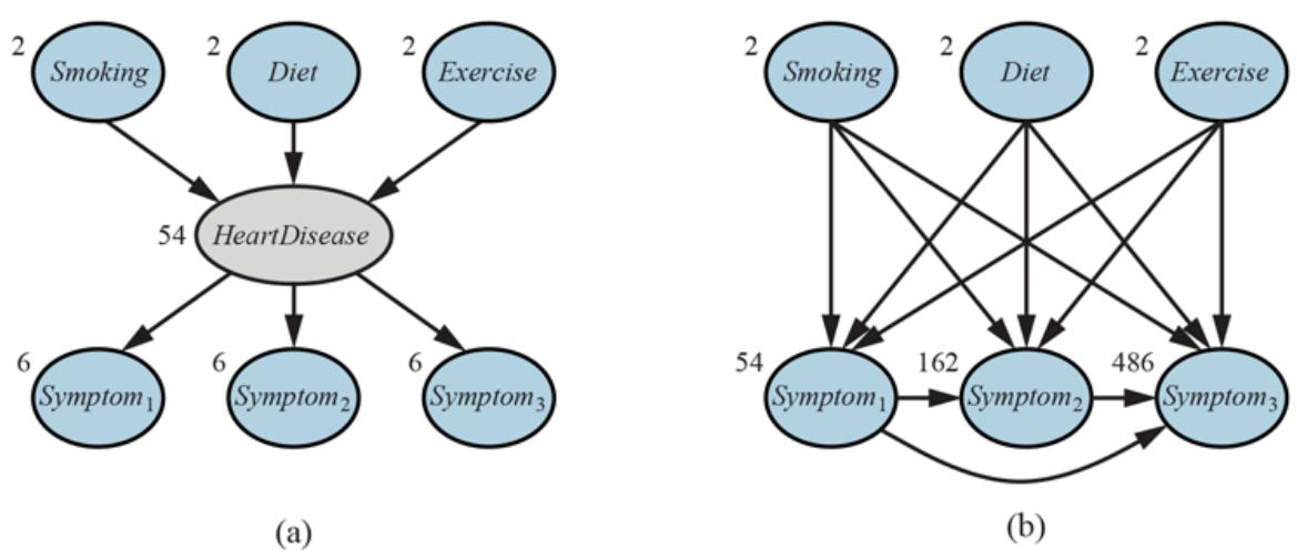
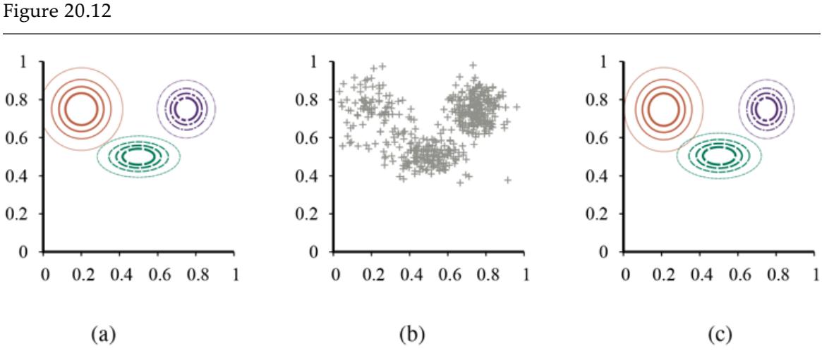
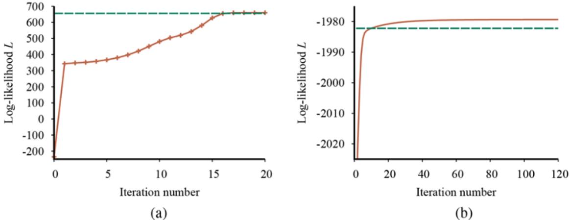
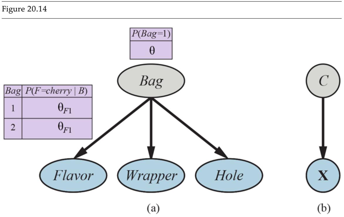
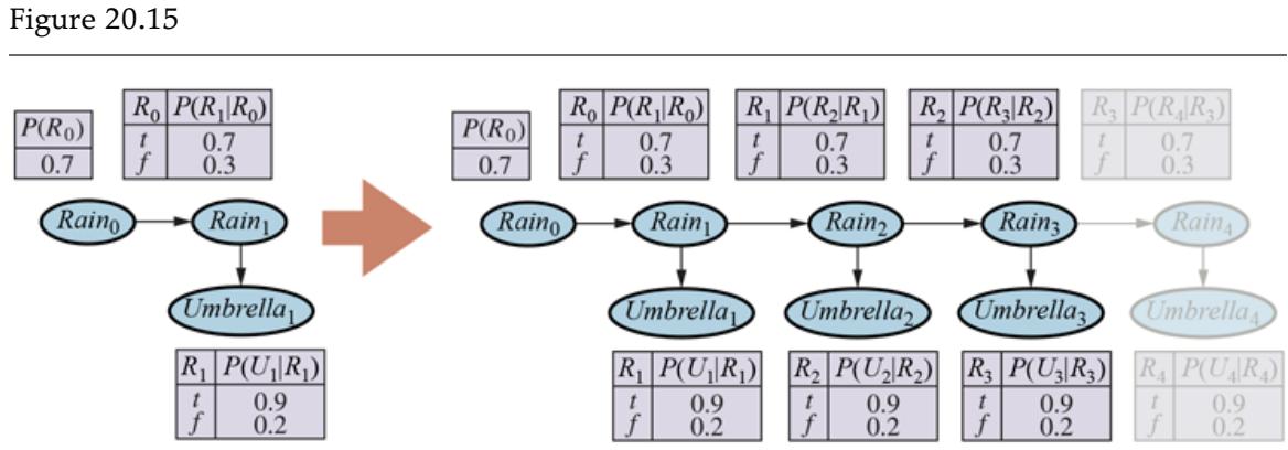
Summary

Statistical learning methods range from simple calculation of averages to the construction of complex models such as Bayesian networks. They have applications throughout computer science, engineering, computational biology, neuroscience, psychology, and physics. This chapter has presented some of the basic ideas and given a flavor of the mathematical underpinnings. The main points are as follows:

• Bayesian learning methods formulate learning as a form of probabilistic inference, using the observations to update a prior distribution over hypotheses. This approach provides a good way to implement Ockham’s razor, but quickly becomes intractable for complex hypothesis spaces.
• Maximum a posteriori (MAP) learning selects a single most likely hypothesis given the data. The hypothesis prior is still used and the method is often more tractable than full Bayesian learning.
• Maximum-likelihood learning simply selects the hypothesis that maximizes the likelihood of the data; it is equivalent to MAP learning with a uniform prior. In simple cases such as linear regression and fully observable Bayesian networks, maximumlikelihood solutions can be found easily in closed form. Naive Bayes learning is a particularly effective technique that scales well.
• When some variables are hidden, local maximum likelihood solutions can be found using the expectation maximization (EM) algorithm. Applications include unsupervised clustering using mixtures of Gaussians, learning Bayesian networks, and learning hidden Markov models.
• Learning the structure of Bayesian networks is an example of model selection. This usually involves a discrete search in the space of structures. Some method is required for trading off model complexity against degree of fit.
• Nonparametric models represent a distribution using the collection of data points. Thus, the number of parameters grows with the training set. Nearest-neighbors methods look at the examples nearest to the point in question, whereas kernel methods form a distance-weighted combination of all the examples.

Statistical learning continues to be a very active area of research. Enormous strides have been made in both theory and practice, to the point where it is possible to learn almost any model for which exact or approximate inference is feasible.

Bibliographical and Historical Notes

The application of statistical learning techniques in AI was an active area of research in the early years (see Duda and Hart, 1973) but became separated from mainstream AI as the latter field concentrated on symbolic methods. A resurgence of interest occurred shortly after the introduction of Bayesian network models in the late 1980s; at roughly the same time, a statistical view of neural network learning began to emerge. In the late 1990s, there was a noticeable convergence of interests in machine learning, statistics, and neural networks, centered on methods for creating large probabilistic models from data.

The naive Bayes model is one of the oldest and simplest forms of Bayesian network, dating back to the 1950s. Its origins were mentioned in Chapter 12 . Its surprising success is partially explained by Domingos and Pazzani (1997). A boosted form of naive Bayes learning won the first KDD Cup data mining competition (Elkan, 1997). Heckerman (1998) gives an excellent introduction to the general problem of Bayes net learning. Bayesian parameter learning with Dirichlet priors for Bayesian networks was discussed by Spiegelhalter et al. (1993). The beta distribution as a conjugate prior for a Bernoulli variable was first derived by Thomas (Bayes, 1763) and later reintroduced by Karl Pearson (1895) as a model for skewed data; for many years it was known as a “Pearson Type I distribution.” Bayesian linear regression is discussed in the text by Box and Tiao (1973); Minka (2010) provides a concise summary of the derivations for the general multivariate case.

Several software packages incorporate mechanisms for statistical learning with Bayes net models. These include BUGS (Bayesian inference Using Gibbs Sampling) (Gilks et al., 1994; Lunn et al., 2000, 2013), JAGS (Just Another Gibbs Sampler) (Plummer, 2003), and STAN (Carpenter et al., 2017).

The first algorithms for learning Bayes net structures used conditional independence tests (Pearl, 1988; Pearl and Verma, 1991). Spirtes et al. (1993) implemented a comprehensive approach in the TETRAD package for Bayes net learning. Algorithmic improvements since then led to a clear victory in the 2001 KDD Cup data mining competition for a Bayes net learning method (Cheng et al., 2002). (The specific task here was a bioinformatics problem with 139,351 features!) A structure-learning approach based on maximizing likelihood was developed by Cooper and Herskovits (1992) and improved by Heckerman et al. (1994).

More recent algorithms have achieved quite respectable performance in the complete-data case (Moore and Wong, 2003; Teyssier and Koller, 2005). One important component is an efficient data structure, the AD-tree, for caching counts over all possible combinations of variables and values (Moore and Lee, 1997). Friedman and Goldszmidt (1996) pointed out the influence of the representation of local conditional distributions on the learned structure.

The general problem of learning probability models with hidden variables and missing data was addressed by Hartley (1958), who described the general idea of what was later called EM and gave several examples. Further impetus came from the Baum–Welch algorithm for HMM learning (Baum and Petrie, 1966), which is a special case of EM. The paper by Dempster, Laird, and Rubin (1977), which presented the EM algorithm in general form and analyzed its convergence, is one of the most cited papers in both computer science and statistics. (Dempster himself views EM as a schema rather than an algorithm, since a good deal of mathematical work may be required before it can be applied to a new family of distributions.) McLachlan and Krishnan (1997) devote an entire book to the algorithm and its properties. The specific problem of learning mixture models, including mixtures of Gaussians, is covered by Titterington et al. (1985).

Within AI, AUTOCLASS (Cheeseman et al., 1988; Cheeseman and Stutz, 1996) was the first successful system that used EM for mixture modeling. AUTOCLASS was applied to a number of real-world scientific classification tasks, including the discovery of new types of stars from spectral data (Goebel et al., 1989) and new classes of proteins and introns in DNA/protein sequence databases (Hunter and States, 1992).

For maximum-likelihood parameter learning in Bayes nets with hidden variables, EM and gradient-based methods were introduced around the same time by Lauritzen (1995) and Russell et al. (1995). The structural EM algorithm was developed by Friedman (1998) and applied to maximum-likelihood learning of Bayes net structures with latent variables. Friedman and Koller (2003) describe Bayesian structure learning. Daly et al. (2011) review the field of Bayes net learning, providing extensive citations to the literature.

The ability to learn the structure of Bayesian networks is closely connected to the issue of recovering causal information from data. That is, is it possible to learn Bayes nets in such a way that the recovered network structure indicates real causal influences? For many years,

statisticians avoided this question, believing that observational data (as opposed to data generated from experimental trials) could yield only correlational information—after all, any two variables that appear related might in fact be influenced by a third, unknown causal factor rather than influencing each other directly. Pearl (2000) has presented convincing arguments to the contrary, showing that there are in fact many cases where causality can be ascertained and developing the causal network formalism to express causes and the effects of intervention as well as ordinary conditional probabilities.

Nonparametric density estimation, also called Parzen window density estimation, was investigated initially by Rosenblatt (1956) and Parzen (1962). Since that time, a huge literature has developed investigating the properties of various estimators. Devroye (1987) gives a thorough introduction. There is also a rapidly growing literature on nonparametric Bayesian methods, originating with the seminal work of Ferguson (1973) on the Dirichlet process, which can be thought of as a distribution over Dirichlet distributions. These methods are particularly useful for mixtures with unknown numbers of components. Ghahramani (2005) and Jordan (2005) provide useful tutorials on the many applications of these ideas to statistical learning. The text by Rasmussen and Williams (2006) covers the Gaussian process, which gives a way of defining prior distributions over the space of continuous functions.

Dirichlet process

Gaussian process

The material in this chapter brings together work from the fields of statistics and pattern recognition, so the story has been told many times in many ways. Good texts on Bayesian statistics include those by DeGroot (1970), Berger (1985), and Gelman et al. (1995). Bishop (2007), Hastie et al. (2009), Barber (2012), and Murphy (2012) provide excellent introductions to statistical machine learning. For pattern classification, the classic text for many years has been Duda and Hart (1973), now updated (Duda et al., 2001). The annual

NeurIPS (Neural Information Processing Systems, formerly NIPS) conference, whose proceedings are published as the series Advances in Neural Information Processing Systems, includes many Bayesian learning papers, as does the annual conference on Artificial Intelligence and Statistics. Specifically Bayesian venues include the Valencia International Meetings on Bayesian Statistics and the journal Bayesian Analysis.

Chapter 21 Deep Learning

In which gradient descent learns multistep programs, with significant implications for the major subfields of artificial intelligence.

Deep learning is a broad family of techniques for machine learning in which hypotheses take the form of complex algebraic circuits with tunable connection strengths. The word “deep” refers to the fact that the circuits are typically organized into many layers, which means that computation paths from inputs to outputs have many steps. Deep learning is currently the most widely used approach for applications such as visual object recognition, machine translation, speech recognition, speech synthesis, and image synthesis; it also plays a significant role in reinforcement learning applications (see Chapter 22 ).

Deep learning

Layer

Deep learning has its origins in early work that tried to model networks of neurons in the brain (McCulloch and Pitts, 1943) with computational circuits. For this reason, the networks trained by deep learning methods are often called neural networks, even though the resemblance to real neural cells and structures is superficial.

Neural network

While the true reasons for the success of deep learning have yet to be fully elucidated, it has self-evident advantages over some of the methods covered in Chapter 19 —particularly for high-dimensional data such as images. For example, although methods such as linear and logistic regression can handle a large number of input variables, the computation path from each input to the output is very short: multiplication by a single weight, then adding into the aggregate output. Moreover, the different input variables contribute independently to the output, without interacting with each other (Figure 21.1(a) ). This significantly limits the expressive power of such models. They can represent only linear functions and boundaries in the input space, whereas most real-world concepts are far more complex.

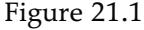
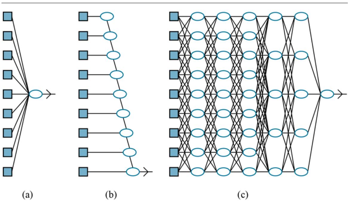
1. A shallow model, such as linear regression, has short computation paths between inputs and output. (b) A decision list network (page 674) has some long paths for some possible input values, but most paths are short. (c) A deep learning network has longer computation paths, allowing each variable to interact with all the others.

Decision lists and decision trees, on the other hand, allow for long computation paths that can depend on many input variables—but only for a relatively small fraction of the possible input vectors (Figure 21.1(b) ). If a decision tree has long computation paths for a significant fraction of the possible inputs, it must be exponentially large in the number of input variables. The basic idea of deep learning is to train circuits such that the computation paths are long, allowing all the input variables to interact in complex ways (Figure

21.1(c) ). These circuit models turn out to be sufficiently expressive to capture the complexity of real-world data for many important kinds of learning problems.

Section 21.1 describes simple feedforward networks, their components, and the essentials of learning in such networks. Section 21.2 goes into more detail on how deep networks are put together, and Section 21.3 covers a class of networks called convolutional neural networks that are especially important in vision applications. Sections 21.4 and 21.5 go into more detail on algorithms for training networks from data and methods for improving generalization. Section 21.6 covers networks with recurrent structure, which are well suited for sequential data. Section 21.7 describes ways to use deep learning for tasks other than supervised learning. Finally, Section 21.8 surveys the range of applications of deep learning.

21.1 Simple Feedforward Networks

A feedforward network, as the name suggests, has connections only in one direction—that is, it forms a directed acyclic graph with designated input and output nodes. Each node computes a function of its inputs and passes the result to its successors in the network. Information flows through the network from the input nodes to the output nodes, and there are no loops. A recurrent network, on the other hand, feeds its intermediate or final outputs back into its own inputs. This means that the signal values within the network form a dynamical system that has internal state or memory. We will consider recurrent networks in Section 21.6 .

Feedforward network

Recurrent network

Boolean circuits, which implement Boolean functions, are an example of feedforward networks. In a Boolean circuit, the inputs are limited to 0 and 1, and each node implements a simple Boolean function of its inputs, producing a 0 or a 1. In neural networks, input values are typically continuous, and nodes take continuous inputs and produce continuous outputs. Some of the inputs to nodes are parameters of the network; the network learns by adjusting the values of these parameters so that the network as a whole fits the training data.

21.1.1 Networks as complex functions

Each node within a network is called a unit. Traditionally, following the design proposed by McCulloch and Pitts, a unit calculates the weighted sum of the inputs from predecessor nodes and then applies a nonlinear function to produce its output. Let denote the output of unit and let be the weight attached to the link from unit to unit ; then we have

\[a\_j = g\_j(\sum\_i w\_{i,j} a\_i) \equiv g\_j(i n\_j),\]

where is a nonlinear activation function associated with unit and is the weighted sum of the inputs to unit .

Activation function

As in Section 19.6.3 (page 679), we stipulate that each unit has an extra input from a dummy unit 0 that is fixed to and a weight for that input. This allows the total weighted input to unit to be nonzero even when the outputs of the preceding layer are all zero. With this convention, we can write the preceding equation in vector form:

(21.1)

\[a\_j = g\_j(\mathbf{w}^\top \mathbf{x})\]

where is the vector of weights leading into unit (including ) and is the vector of inputs to unit (including the ).

The fact that the activation function is nonlinear is important because if it were not, any composition of units would still represent a linear function. The nonlinearity is what allows sufficiently large networks of units to represent arbitrary functions. The universal approximation theorem states that a network with just two layers of computational units, the first nonlinear and the second linear, can approximate any continuous function to an arbitrary degree of accuracy. The proof works by showing that an exponentially large network can represent exponentially many “bumps” of different heights at different locations in the input space, thereby approximating the desired function. In other words,

sufficiently large networks can implement a lookup table for continuous functions, just as sufficiently large decision trees implement a lookup table for Boolean functions.

A variety of different activation functions are used. The most common are the following:

The logistic or sigmoid function, which is also used in logistic regression (see page 685):

\[ \sigma(x) = 1/(1 + e^{-x})\,. \]

Sigmoid

The ReLU function, whose name is an abbreviation for rectified linear unit:

\[\text{ReLU}(x) = \max(0, x).\]

ReLU

The softplus function, a smooth version of the ReLU function:

\[\text{softplus}(x) = \log(1 + e^x).\]

Softplus

The derivative of the softplus function is the sigmoid function.

The tanh function:

\[\tanh(x) = \frac{e^{2x} - 1}{e^{2x} + 1}.\]

Note that the range of tanh is . Tanh is a scaled and shifted version of the sigmoid, as .

These functions are shown in Figure 21.2 . Notice that all of them are monotonically nondecreasing, which means that their derivatives are nonnegative. We will have more to say about the choice of activation function in later sections.

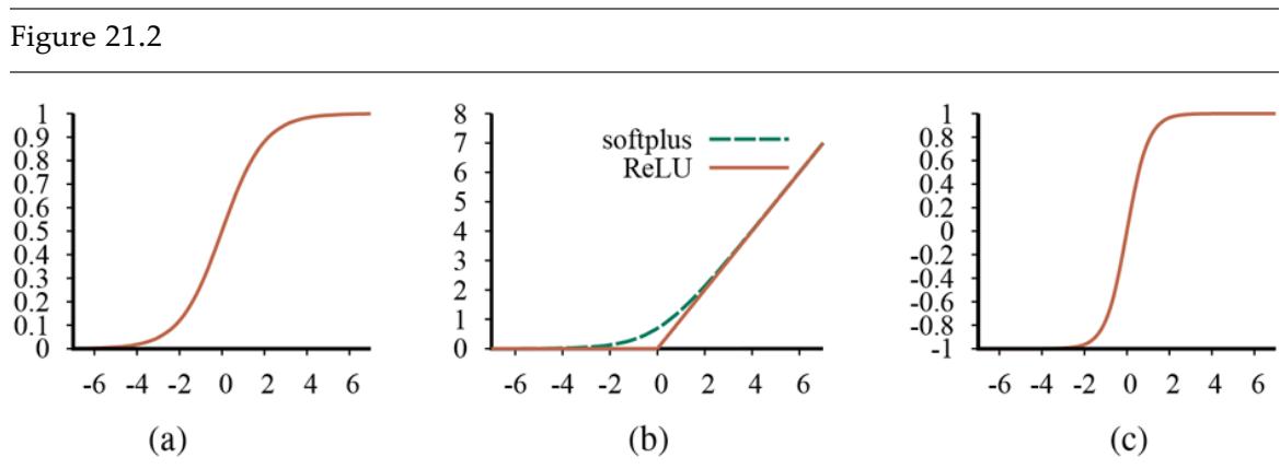
Activation functions commonly used in deep learning systems: (a) the logistic or sigmoid function; (b) the ReLU function and the softplus function; (c) the tanh function.

Coupling multiple units together into a network creates a complex function that is a composition of the algebraic expressions represented by the individual units. For example, the network shown in Figure 21.3(a) represents a function , parameterized by weights , that maps a two-element input vector to a scalar output value . The internal structure of the function mirrors the structure of the network. For example, we can write an expression for the output as follows:

(21.2)

\[\begin{aligned} \hat{y} &= g\_5(in\_5) = g\_5(w\_{0,5} + w\_{3,5}a\_3 + w\_{4,5}a\_4) \\ &= g\_5(w\_{0,5} + w\_{3,5}g\_3(in\_3) + w\_{4,5}g\_4(in\_4)) \\ &= g\_5(w\_{0,5} + w\_{3,5}g\_3(w\_{0,3} + w\_{1,3}x\_1 + w\_{2,3}x\_2) \\ &\quad + w\_{4,5}g\_4(w\_{0,4} + w\_{1,4}x\_1 + w\_{2,4}x\_2)). \end{aligned}\]

Tanh

1. A neural network with two inputs, one hidden layer of two units, and one output unit. Not shown are the dummy inputs and their associated weights. (b) The network in (a) unpacked into its full computation graph.

Thus, we have the output expressed as a function of the inputs and the weights.

Figure 21.3(a) shows the traditional way a network might be depicted in a book on neural networks. A more general way to think about the network is as a computation graph or dataflow graph—essentially a circuit in which each node represents an elementary computation. Figure 21.3(b) shows the computation graph corresponding to the network in Figure 21.3(a) ; the graph makes each element of the overall computation explicit. It also distinguishes between the inputs (in blue) and the weights (in light mauve): the weights can be adjusted to make the output agree more closely with the true value in the training data. Each weight is like a volume control knob that determines how much the next node in the graph hears from that particular predecessor in the graph.

Computation graph

Just as Equation (21.1) described the operation of a unit in vector form, we can do something similar for the network as a whole. We will generally use to denote a weight matrix; for this network, denotes the weights in the first layer ( , , etc.) and denotes the weights in the second layer ( etc.). Finally, let and denote the activation functions in the first and second layers. Then the entire network can be written as follows:

(21.3)

\[h\_{\mathbf{w}}(\mathbf{x}) = \mathbf{g}^{(2)}(\mathbf{W}^{(2)}\mathbf{g}^{(1)}(\mathbf{W}^{(1)}\mathbf{x})).\]

Like Equation (21.2) , this expression corresponds to a computation graph, albeit a much simpler one than the graph in Figure 21.3(b) : here, the graph is simply a chain with weight matrices feeding into each layer.

The computation graph in Figure 21.3(b) is relatively small and shallow, but the same idea applies to all forms of deep learning: we construct computation graphs and adjust their weights to fit the data. The graph in Figure 21.3(b) is also fully connected, meaning that every node in each layer is connected to every node in the next layer. This is in some sense the default, but we will see in Section 21.3 that choosing the connectivity of the network is also important in achieving effective learning.

Fully connected

21.1.2 Gradients and learning

In Section 19.6 , we introduced an approach to supervised learning based on gradient descent: calculate the gradient of the loss function with respect to the weights, and adjust the weights along the gradient direction to reduce the loss. (If you have not already read

Section 19.6 , we recommend strongly that you do so before continuing.) We can apply exactly the same approach to learning the weights in computation graphs. For the weights leading into units in the output layer—the ones that produce the output of the network, the gradient calculation is essentially identical to the process in Section 19.6 . For weights leading into units in the hidden layers, which are not directly connected to the outputs, the process is only slightly more complicated.

Output layer

Hidden layer

For now, we will use the squared loss function, , and we will calculate the gradient for the network in Figure 21.3 with respect to a single training example . (For multiple examples, the gradient is just the sum of the gradients for the individual examples.) The network outputs a prediction and the true value is , so we have

\[Loss(h\_{\mathbf{w}}) = L\_2(y, h\_{\mathbf{w}}(\mathbf{x})) = ||y - h\_{\mathbf{w}}(\mathbf{x})||^2 = (y - \hat{y})^2.\]

To compute the gradient of the loss with respect to the weights, we need the same tools of calculus we used in Chapter 19 —principally the chain rule, . We’ll start with the easy case: a weight such as that is connected to the output unit. We operate directly on the network-defining expressions from Equation (21.2) :

(21.4)

\[\begin{split} \frac{\partial}{\partial w\_{3,5}} Loss(h\_{\mathbf{w}}) &= \frac{\partial}{\partial w\_{3,5}} (y - \hat{y})^2 = -2(y - \hat{y}) \frac{\partial \hat{y}}{\partial w\_{3,5}} \\ &= -2(y - \hat{y}) \frac{\partial}{\partial w\_{3,5}} g\_5(in\_5) = -2(y - \hat{y}) g\_5'(in\_5) \frac{\partial}{\partial w\_{3,5}} in\_5 \\ &= -2(y - \hat{y}) g\_5'(in\_5) \frac{\partial}{\partial w\_{3,5}} (w\_{0,5} + w\_{3,5} a\_3 + w\_{4,5} a\_4) \\ &= -2(y - \hat{y}) g\_5'(in\_5) a\_3. \end{split}\]

The simplification in the last line follows because and do not depend on , nor does the coefficient of , .

The slightly more difficult case involves a weight such as that is not directly connected to the output unit. Here, we have to apply the chain rule one more time. The first few steps are identical, so we omit them:

(21.5)

\[\begin{split} \frac{\partial}{\partial w\_{1,3}} Loss(h\_{\mathbf{w}}) &= -2(y - \hat{y})g\_5'(in\_5) \frac{\partial}{\partial w\_{1,3}} \left( w\_{0,5} + w\_{3,5} a\_3 + w\_{4,5} a\_4 \right) \\ &= -2(y - \hat{y})g\_5'(in\_5) w\_{3,5} \frac{\partial}{\partial w\_{1,3}} a\_3 \\ &= -2(y - \hat{y})g\_5'(in\_5) w\_{3,5} \frac{\partial}{\partial w\_{1,3}} g\_3(in\_3) \\ &= -2(y - \hat{y})g\_5'(in\_5) w\_{3,5} g\_3'(in\_3) \frac{\partial}{\partial w\_{1,3}} in\_3 \\ &= -2(y - \hat{y})g\_5'(in\_5) w\_{3,5} g\_3'(in\_3) \frac{\partial}{\partial w\_{1,3}} (w\_{0,3} + w\_{1,3} x\_1 + w\_{2,3} x\_2) \\ &= -2(y - \hat{y})g\_5'(in\_5) w\_{3,5} g\_3'(in\_3) x\_1. \end{split}\]

So, we have fairly simple expressions for the gradient of the loss with respect to the weights and .

If we define as a sort of “perceived error” at the point where unit 5 receives its input, then the gradient with respect to is just . This makes perfect sense: if is positive, that means is too big (recall that is always nonnegative); if is also positive, then increasing will only make things worse, whereas if is negative, then increasing will reduce the error. The magnitude of also matters: if is small for this training example, then didn’t play a major role in producing the error and doesn’t need to be changed much.

If we also define , then the gradient for becomes just . Thus, the perceived error at the input to unit 3 is the perceived error at the input to unit 5, multiplied by information along the path from 5 back to 3. This phenomenon is completely general, and gives rise to the term back-propagation for the way that the error at the output is passed back through the network.

Back-propagation

Another important characteristic of these gradient expressions is that they have as factors the local derivatives . As noted earlier, these derivatives are always nonnegative, but they can be very close to zero (in the case of the sigmoid, softplus, and tanh functions) or exactly zero (in the case of ReLUs), if the inputs from the training example in question happen to put unit in the flat operating region. If the derivative is small or zero, that means that changing the weights leading into unit will have a negligible effect on its output. As a result, deep networks with many layers may suffer from a vanishing gradient the error signals are extinguished altogether as they are propagated back through the network. Section 21.3.3 provides one solution to this problem.

Vanishing gradient

We have shown that gradients in our tiny example network are simple expressions that can be computed by passing information back through the network from the output units. It turns out that this property holds more generally. In fact, as we show in Section 21.4.1 , the gradient computations for any feedforward computation graph have the same structure as the underlying computation graph. This property follows straightforwardly from the rules of differentiation.

We have shown the gory details of a gradient calculation, but worry not: there is no need to redo the derivations in Equations (21.4) and (21.5) for each new network structure! All

such gradients can be computed by the method of automatic differentiation, which applies the rules of calculus in a systematic way to calculate gradients for any numeric program. In fact, the method of back-propagation in deep learning is simply an application of reverse mode differentiation, which applies the chain rule “from the outside in” and gains the efficiency advantages of dynamic programming when the network in question has many inputs and relatively few outputs. 1

1 Automatic differentiation methods were originally developed in the 1960s and 1970s for optimizing the parameters of systems defined by large, complex Fortran programs.

Automatic differentiation

Reverse mode

All of the major packages for deep learning provide automatic differentiation, so that users can experiment freely with different network structures, activation functions, loss functions, and forms of composition without having to do lots of calculus to derive a new learning algorithm for each experiment. This has encouraged an approach called end-to-end learning, in which a complex computational system for a task such as machine translation can be composed from several trainable subsystems; the entire system is then trained in an end-to-end fashion from input/output pairs. With this approach, the designer need have only a vague idea about how the overall system should be structured; there is no need to know in advance exactly what each subsystem should do or how to label its inputs and outputs.

End-to-end learning

21.2 Computation Graphs for Deep Learning

We have established the basic ideas of deep learning: represent hypotheses as computation graphs with tunable weights and compute the gradient of the loss function with respect to those weights in order to fit the training data. Now we look at how to put together computation graphs. We begin with the input layer, which is where the training or test example is encoded as values of the input nodes. Then we consider the output layer, where the outputs are compared with the true values to derive a learning signal for tuning the weights. Finally, we look at the hidden layers of the network.

21.2.1 Input encoding

The input and output nodes of a computational graph are the ones that connect directly to the input data and the output data . The encoding of input data is usually straightforward, at least for the case of factored data where each training example contains values for input attributes. If the attributes are Boolean, we have input nodes; usually is mapped to an input of 0 and is mapped to 1, although sometimes and are used. Numeric attributes, whether integer or real-valued, are typically used as is, although they may be scaled to fit within a fixed range; if the magnitudes for different examples vary enormously, the values can be mapped onto a log scale.

Images do not quite fit into the category of factored data; although an RGB image of size pixels can be thought of as integer-valued attributes (typically with values in the range ), this would ignore the fact that the RGB triplets belong to the same pixel in the image and the fact that pixel adjacency really matters. Of course, we can map adjacent pixels onto adjacent input nodes in the network, but the meaning of adjacency is completely lost if the internal layers of the network are fully connected. In practice, networks used with image data have array-like internal structures that aim to reflect the semantics of adjacency. We will see this in more detail in Section 21.3 .

Categorical attributes with more than two values—like the attribute in the restaurant problem from Chapter 19 , which has values French, Italian, Thai, or burger)—are usually encoded using the so-called one-hot encoding. An attribute with possible values is represented by separate input bits. For any given value, the corresponding input bit is set to 1 and all the others are set to 0. This generally works better than mapping the values to integers. If we used integers for the attribute, Thai would be 3 and burger would be 4. Because the network is a composition of continuous functions, it would have no choice but to pay attention to numerical adjacency, but in this case the numerical adjacency between Thai and burger is semantically meaningless.

21.2.2 Output layers and loss functions

On the output side of the network, the problem of encoding the raw data values into actual values for the output nodes of the graph is much the same as the input encoding problem. For example, if the network is trying to predict the Weather variable from Chapter 12 , which has values {sun, rain, cloud, snow}, we would use a one-hot encoding with four bits.

So much for the data values . What about the prediction ? Ideally, it would exactly match the desired value , and the loss would be zero, and we’d be done. In practice, this seldom happens—especially before we have started the process of adjusting the weights! Thus, we need to think about what an incorrect output value means, and how to measure the loss. In deriving the gradients in Equations (21.4) and (21.5) , we began with the squared-error loss function. This keeps the algebra simple, but it is not the only possibility. In fact, for most deep learning applications, it is more common to interpret the output values as probabilities and to use the negative log likelihood as the loss function—exactly as we did with maximum likelihood learning in Chapter 20 .

Maximum likelihood learning finds the value of that maximizes the probability of the observed data. And because the log function is monotonic, this is equivalent to maximizing the log likelihood of the data, which is equivalent in turn to minimizing a loss function defined as the negative log likelihood. (Recall from page 725 that taking logs turns products of probabilities into sums, which are more amenable for taking derivatives.) In other words, we are looking for that minimizes the sum of negative log probabilities of the examples:

(21.6)

\[\mathbf{w}^\* = \underset{\mathbf{w}}{\text{argmin}} - \sum\_{j=1}^N \log P\_{\mathbf{w}}(\mathbf{y}\_j|\mathbf{x}\_j).\]

In the deep learning literature, it is common to talk about minimizing the cross-entropy loss. Cross-entropy, written as , is a kind of measure of dissimilarity between two distributions and . The general definition is 2

2 Cross-entropy is not a distance in the usual sense because is not zero; rather, it equals the entropy . It is easy to show that , where is the Kullback–Leibler divergence, which does satisfy . Thus, for fixed , varying to minimize the cross-entropy also minimizes the KL divergence.

Cross-entropy

(21.7)

\[H(P,Q) = \mathbf{E}\_{\mathbf{z}\sim P(\mathbf{z})}[\log Q(\mathbf{z})] = \int P(\mathbf{z}) \log Q(\mathbf{z}) d\mathbf{z}.\]

In machine learning, we typically use this definition with being the true distribution over training examples, , and being the predictive hypothesis . Minimizing the cross-entropy by adjusting makes the hypothesis agree as closely as possible with the true distribution. In reality, we cannot minimize this cross-entropy because we do not have access to the true data distribution ; but we do have access to samples from , so the sum over the actual data in Equation (21.6) approximates the expectation in Equation (21.7) .

To minimize the negative log likelihood (or the cross-entropy), we need to be able to interpret the output of the network as a probability. For example, if the network has one output unit with a sigmoid activation function and is learning a Boolean classification, we can interpret the output value directly as the probability that the example belongs to the positive class. (Indeed, this is exactly how logistic regression is used; see page 684.) Thus, for Boolean classification problems, we commonly use a sigmoid output layer.

Multiclass classification problems are very common in machine learning. For example, classifiers used for object recognition often need to recognize thousands of distinct categories of objects. Natural language models that try to predict the next word in a sentence may have to choose among tens of thousands of possible words. For this kind of prediction, we need the network to output a categorical distribution—that is, if there are possible answers, we need output nodes that represent probabilities summing to 1.

To achieve this, we use a softmax layer, which outputs a vector of values given a vector of input values . The th element of that output vector is given by

\[\text{softmax}(\mathbf{in})\_k = \frac{e^{in\_k}}{\sum\_{k'=1}^d e^{in\_{k'}}}.\]

Softmax

By construction, the softmax function outputs a vector of nonnegative numbers that sum to 1. As usual, the input to each of the output nodes will be a weighted linear combination of the outputs of the preceding layer. Because of the exponentials, the softmax layer accentuates differences in the inputs: for example, if the vector of inputs is given by , then the outputs are . The softmax, is, nonetheless, smooth and differentiable (Exercise 21.SOFG), unlike the function. It is easy to show (Exercise 21.SMSG) that the sigmoid is a softmax with . In other words, just as sigmoid units propagate binary class information through a network, softmax units propagate multiclass information.

For a regression problem, where the target value is continuous, it is common to use a linear output layer—in other words, , without any activation function —and to interpret this as the mean of a Gaussian prediction with fixed variance. As we noted on page 729, maximizing likelihood (i.e., minimizing negative log likelihood) with a fixed-variance Gaussian is the same as minimizing squared error. Thus, a linear output layer interpreted in this way does classical linear regression. The input features to this linear regression are the outputs from the preceding layer, which typically result from multiple nonlinear transformations of the original inputs to the network.

Many other output layers are possible. For example, a mixture density layer represents the outputs using a mixture of Gaussian distributions. (See Section 20.3.1 for more details on

Gaussian mixtures.) Such layers predict the relative frequency of each mixture component, the mean of each component, and the variance of each component. As long as these output values are interpreted appropriately by the loss function as defining the probability for the true output value , the network will, after training, fit a Gaussian mixture model in the space of features defined by the preceding layers.

Mixture density

21.2.3 Hidden layers

During the training process, a neural network is shown many input values and many corresponding output values . While processing an input vector , the neural network performs several intermediate computations before producing the output . We can think of the values computed at each layer of the network as a different representation for the input . Each layer transforms the representation produced by the preceding layer to produce a new representation. The composition of all these transformations succeeds—if all goes well—in transforming the input into the desired output. Indeed, one hypothesis for why deep learning works well is that the complex end-to-end transformation that maps from input to output—say, from an input image to the output category “giraffe”—is decomposed by the many layers into the composition of many relatively simple transformations, each of which is fairly easy to learn by a local updating process.

In the process of forming all these internal transformations, deep networks often discover meaningful intermediate representations of the data. For example, a network learning to recognize complex objects in images may form internal layers that detect useful subunits: edges, corners, ellipses, eyes, faces—cats. Or it may not—deep networks may form internal layers whose meaning is opaque to humans, even though the output is still correct.

The hidden layers of neural networks are typically less diverse than the output layers. For the first 25 years of research with multilayer networks (roughly 1985–2010), internal nodes used sigmoid and tanh activation functions almost exclusively. From around 2010 onwards, the ReLU and softplus become more popular, partly because they are believed to avoid the problem of vanishing gradients mentioned in Section 21.1.2 . Experimentation with

increasingly deep networks suggested that, in many cases, better learning was obtained with deep and relatively narrow networks rather than shallow, wide networks, given a fixed total number of weights. A typical example of this is shown in Figure 21.7 on page 769.

Test-set error as a function of layer width (as measured by total number of weights) for three-layer and eleven-layer convolutional networks. The data come from early versions of Google’s system for transcribing addresses in photos taken by Street View cars (Goodfellow et al., 2014).

There are, of course, many other structures to consider for computation graphs, besides just playing with width and depth. At the time of writing, there is little understanding as to why some structures seem to work better than others for some particular problem. With experience, practitioners gain some intuition as to how to design networks and how to fix them when they don’t work, just as chefs gain intuition for how to design recipes and how to fix them when they taste unpleasant. For this reason, tools that facilitate rapid exploration and evaluation of different structures are essential for success in real-world problems.

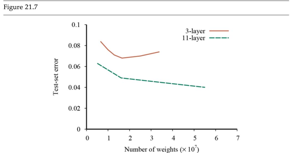
21.3 Convolutional Networks

We mentioned in Section 21.2.1 that an image cannot be thought of as a simple vector of input pixel values, primarily because adjacency of pixels really matters. If we were to construct a network with fully connected layers and an image as input, we would get the same result whether we trained with unperturbed images or with images all of whose pixels had been randomly permuted. Furthermore, suppose there are pixels and units in the first hidden layer, to which the pixels provide input. If the input and the first hidden layer are fully connected, that means weights; for a typical megapixel RGB image, that’s 9 trillion weights. Such a vast parameter space would require correspondingly vast numbers of training images and a huge computational budget to run the training algorithm.

These considerations suggest that we should construct the first hidden layer so that each hidden unit receives input from only a small, local region of the image. This kills two birds with one stone. First, it respects adjacency, at least locally. (And we will see later that if subsequent layers have the same locality property, then the network will respect adjacency in a global sense.) Second, it cuts down the number of weights: if each local region has pixels, then there will be weights in all.

So far, so good. But we are missing another important property of images: roughly speaking, anything that is detectable in one small, local region of the image—perhaps an eye or a blade of grass—would look the same if it appeared in another small, local region of the image. In other words, we expect image data to exhibit approximate spatial invariance, at least at small to moderate scales. We don’t necessarily expect the top halves of photos to look like bottom halves, so there is a scale beyond which spatial invariance no longer holds. 3

3 Similar ideas can be applied to process time-series data sources such as audio waveforms. These typically exhibit temporal invariance—a word sounds the same no matter what time of day it is uttered. Recurrent neural networks (Section 21.6 ) automatically exhibit temporal invariance.

Spatial invariance

Local spatial invariance can be achieved by constraining the weights connecting a local region to a unit in the hidden layer to be the same for each hidden unit. (That is, for hidden units and , the weights are the same as .) This makes the hidden units into feature detectors that detect the same feature wherever it appear in the image. Typically, we want the first hidden layer to detect many kinds of features, not just one; so for each local image region we might have hidden units with distinct sets of weights. This means that there are weights in all—a number that is not only far smaller than , but is actually independent of , the image size. Thus, by injecting some prior knowledge namely, knowledge of adjacency and spatial invariance—we can develop models that have far fewer parameters and can learn much more quickly.

A convolutional neural network (CNN) is one that contains spatially local connections, at least in the early layers, and has patterns of weights that are replicated across the units in each layer. A pattern of weights that is replicated across multiple local regions is called a kernel and the process of applying the kernel to the pixels of the image (or to spatially organized units in a subsequent layer) is called convolution. 4

4 In the terminology of signal processing, we would call this operation a cross-correlation, not a convolution. But “convolution” is used within the field of neural networks.

Convolutional neural network (CNN)

Kernel

Convolution

Kernels and convolutions are easiest to illustrate in one dimension rather than two or more, so we will assume an input vector of size , corresponding to pixels in a onedimensional image, and a vector kernel of size . (For simplicity we will assume that is an odd number.) All the ideas carry over straightforwardly to higher-dimensional cases.

We write the convolution operation using the symbol, for example: . The operation is defined as follows:

(21.8)

\[z\_i = \sum\_{j=1}^{l} k\_j x\_{j+i - (l+1)/2}.\]

In other words, for each output position , we take the dot product between the kernel and a snippet of centered on with width .

The process is illustrated in Figure 21.4 for a kernel vector , which detects a darker point in the 1D image. (The 2D version might detect a darker line.) Notice that in this example the pixels on which the kernels are centered are separated by a distance of 2 pixels; we say the kernel is applied with a stride . Notice that the output layer has fewer pixels: because of the stride, the number of pixels is reduced from to roughly . (In two dimensions, the number of pixels would be roughly , where and are the strides in the and directions in the image.) We say “roughly” because of what happens at the edge of the image: in Figure 21.4 the convolution stops at the edges of the image, but one can also pad the input with extra pixels (either zeroes or copies of the outer pixels) so that the kernel can be applied exactly times. For small kernels, we typically use , so the output has the same dimensions as the image (see Figure 21.5 ).

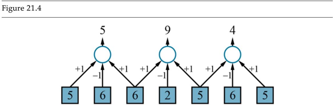
An example of a one-dimensional convolution operation with a kernel of size and a stride . The peak response is centered on the darker (lower intensity) input pixel. The results would usually be fed through a nonlinear activation function (not shown) before going to the next hidden layer.

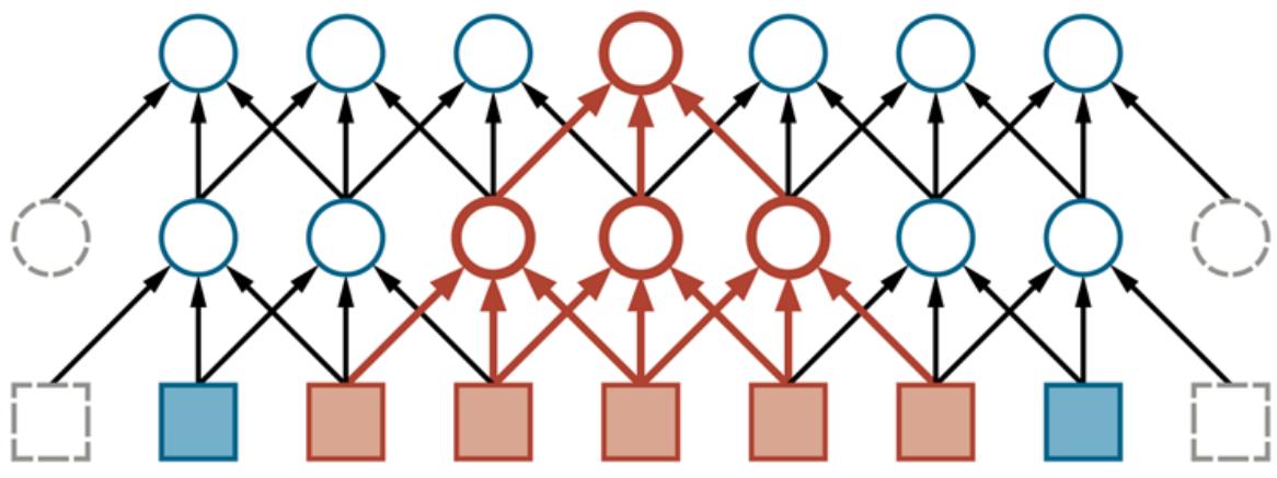
The first two layers of a CNN for a 1D image with a kernel size and a stride . Padding is added at the left and right ends in order to keep the hidden layers the same size as the input. Shown in red is the receptive field of a unit in the second hidden layer. Generally speaking, the deeper the unit, the larger the receptive field.

Stride

The operation of applying a kernel across an image can be implemented in the obvious way by a program with suitable nested loops; but it can also be formulated as a single matrix operation, just like the application of the weight matrix in Equation (21.1) . For example, the convolution illustrated in Figure 21.4 can be viewed as the following matrix multiplication:

(21.9)

\[ \begin{pmatrix} +1 & -1 & +1 & 0 & 0 & 0 & 0 \\ 0 & 0 & +1 & -1 & +1 & 0 & 0 \\ 0 & 0 & 0 & 0 & +1 & -1 & +1 \end{pmatrix} \begin{pmatrix} 5 \\ 6 \\ 6 \\ 2 \\ 5 \\ 6 \\ 6 \\ 5 \end{pmatrix} = \begin{pmatrix} 5 \\ 9 \\ 4 \end{pmatrix}. \]

In this weight matrix, the kernel appears in each row, shifted according to the stride relative to the previous row, One wouldn’t necessarily construct the weight matrix explicitly—it is

mostly zeroes, after all—but the fact that convolution is a linear matrix operation serves as a reminder that gradient descent can be applied easily and effectively to CNNs, just as it can to plain vanilla neural networks.

As mentioned earlier, there will be kernels, not just one; so, with a stride of 1, the output will be times larger. This means that a two-dimensional input array becomes a threedimensional array of hidden units, where the third dimension is of size . It is important to organize the hidden layer this way, so that all the kernel outputs from a particular image location stay associated with that location. Unlike the spatial dimensions of the image, however, this additional “kernel dimension” does not have any adjacency properties, so it does not make sense to run convolutions along it.

CNNs were inspired originally by models of the visual cortex proposed in neuroscience. In those models, the receptive field of a neuron is the portion of the sensory input that can affect that neuron’s activation. In a CNN, the receptive field of a unit in the first hidden layer is small—just the size of the kernel, i.e., pixels. In the deeper layers of the network, it can be much larger. Figure 21.5 illustrates this for a unit in the second hidden layer, whose receptive field contains five pixels. When the stride is 1, as in the figure, a node in the th hidden layer will have a receptive field of size ; so the growth is linear in . (In a 2D image, each dimension of the receptive field grows linearly with , so the area grows quadratically.) When the stride is larger than 1, each pixel in layer represents pixels in layer ; therefore, the receptive field grows as —that is, exponentially with depth. The same effect occurs with pooling layers, which we discuss next.

Receptive field

21.3.1 Pooling and downsampling

A pooling layer in a neural network summarizes a set of adjacent units from the preceding layer with a single value. Pooling works just like a convolution layer, with a kernel size and stride , but the operation that is applied is fixed rather than learned. Typically, no activation function is associated with the pooling layer. There are two common forms of pooling:

Pooling

Downsampling

• Average-pooling computes the average value of its inputs. This is identical to convolution with a uniform kernel vector . If we set , the effect is to coarsen the resolution of the image—to downsample it—by a factor of . An object that occupied, say, pixels would now occupy only pixels after pooling. The same learned classifier that would be able to recognize the object at a size of 10 pixels in the original image would now be able to recognize that object in the pooled image, even if it was too big to recognize in the original image. In other words, average-pooling facilitates multiscale recognition. It also reduces the number of weights required in subsequent layers, leading to lower computational cost and possibly faster learning.
• Max-pooling computes the maximum value of its inputs. It can also be used purely for downsampling, but it has a somewhat different semantics. Suppose we applied maxpooling to the hidden layer in Figure 21.4 : the result would be a 9, indicating that somewhere in the input image there is a darker dot that is detected by the kernel. In other words, max-pooling acts as a kind of logical disjunction, saying that a feature exists somewhere in the unit’s receptive field.

If the goal is to classify the image into one of categories, then the final layer of the network will be a softmax with output units. The early layers of the CNN are image-sized, so somewhere in between there must be significant reductions in layer size. Convolution layers and pooling layers with stride larger than 1 all serve to reduce the layer size. It’s also possible to reduce the layer size simply by having a fully connected layer with fewer units than the preceding layer. CNNs often have one or two such layers preceding the final softmax layer.

21.3.2 Tensor operations in CNNs

We saw in Equations (21.1) and (21.3) that the use of vector and matrix notation can be helpful in keeping mathematical derivations simple and elegant and providing concise

descriptions of computation graphs. Vectors and matrices are one-dimensional and twodimensional special cases of tensors, which (in deep learning terminology) are simply multidimensional arrays of any dimension. 5

5 The proper mathematical definition of tensors requires that certain invariances hold under a change of basis.

Tensor

For CNNs, tensors are a way of keeping track of the “shape” of the data as it progresses through the layers of the network. This is important because the whole notion of convolution depends on the idea of adjacency: adjacent data elements are assumed to be semantically related, so it makes sense to apply operators to local regions of the data. Moreover, with suitable language primitives for constructing tensors and applying operators, the layers themselves can be described concisely as maps from tensor inputs to tensor outputs.

A final reason for describing CNNs in terms of tensor operations is computational efficiency: given a description of a network as a sequence of tensor operations, a deep learning software package can generate compiled code that is highly optimized for the underlying computational substrate. Deep learning workloads are often run on GPUs (graphics processing units) or TPUs (tensor processing units), which make available a high degree of parallelism. For example, one of Google’s third-generation TPU pods has throughput equivalent to about ten million laptops. Taking advantage of these capabilities is essential if one is training a large CNN on a large database of images. Thus, it is common to process not one image at a time but many images in parallel; as we will see in Section 21.4 , this also aligns nicely with the way that the stochastic gradient descent algorithm calculates gradients with respect to a minibatch of training examples.

Let us put all this together in the form of an example. Suppose we are training on RGB images with a minibatch size of 64. The input in this case will be a four-dimensional tensor of size . Then we apply 96 kernels of size with a stride of 2 in both and directions in the image. This gives an output tensor of size

. Such a tensor is often called a feature map, since it shows how each feature extracted by a kernel appears across the entire image; in this case it is composed of 96 channels, where each channel carries information from one feature. Notice that unlike the input tensor, this feature map no longer has dedicated color channels; nonetheless, the color information may still be present in the various feature channels if the learning algorithm finds color to be useful for the final predictions of the network.

Feature map

Channel

21.3.3 Residual networks

Residual networks are a popular and successful approach to building very deep networks that avoid the problem of vanishing gradients.

Residual network

Typical deep models use layers that learn a new representation at layer by completely replacing the representation at layer . Using the matrix–vector notation that we introduced in Equation (21.3) , with being the values of the units in layer , we have

\[\mathbf{z}^{(i)} = f(\mathbf{z}^{(i-1)}) = \mathbf{g}^{(i)}(\mathbf{W}^{(i)}\mathbf{z}^{(i-1)}) .\]

Because each layer completely replaces the representation from the preceding layer, all of the layers must learn to do something useful. Each layer must, at the very least, preserve the task-relevant information contained in the preceding layer. If we set for any layer , the entire network ceases to function. If we also set , the network would not even

be able to learn: layer would not learn because it would observe no variation in its input from layer , and layer would not learn because the back-propagated gradient from layer would always be zero. Of course, these are extreme examples, but they illustrate the need for layers to serve as conduits for the signals passing through the network.

The key idea of residual networks is that a layer should perturb the representation from the previous layer rather than replace it entirely. If the learned perturbation is small, the next layer is close to being a copy of the previous layer. This is achieved by the following equation for layer in terms of layer :

(21.10)

\[\mathbf{z}^{(i)} = \mathbf{g}\_r^{(i)} (\mathbf{z}^{(i-1)} + f(\mathbf{z}^{(i-1)})),\]

where denotes the activation functions for the residual layer. Here we think of as the residual, perturbing the default behavior of passing layer through to layer . The function used to compute the residual is typically a neural network with one nonlinear layer combined with one linear layer:

\[f(\mathbf{z}) = \mathbf{V}\mathbf{g}(\mathbf{W}\mathbf{z}),\]

Residual

where and are learned weight matrices with the usual bias weights added.

Residual networks make it possible to learn significantly deeper networks reliably. Consider what happens if we set for a particular layer in order to disable that layer. Then the residual disappears and Equation (21.10) simplifies to

\[\mathbf{z}^{(i)} = \mathbf{g}\_r(\mathbf{z}^{(i-1)}).\]

Now suppose that consists of ReLU activation functions and that also applies a ReLU function to its inputs: . In that case we have

\[\mathbf{z}^{(i)} = \mathbf{g}\_r(\mathbf{z}^{(i-1)}) = \text{ReLU}(\mathbf{z}^{(i-1)}) = \text{ReLU}(\text{ReLU}(\mathbf{in}^{(i-1)})) = \text{ReLU}(\mathbf{in}^{(i-1)}) = \mathbf{z}^{(i-1)},\]

where the penultimate step follows because . In other words, in residual nets with ReLU activations, a layer with zero weights simply passes its inputs through with no change. The rest of the network functions just as if the layer had never existed. Whereas traditional networks must learn to propagate information and are subject to catastrophic failure of information propagation for bad choices of the parameters, residual networks propagate information by default.

Residual networks are often used with convolutional layers in vision applications, but they are in fact a general-purpose tool that makes deep networks more robust and allows researchers to experiment more freely with complex and heterogeneous network designs. At the time of writing, it is not uncommon to see residual networks with hundreds of layers. The design of such networks is evolving rapidly, so any additional specifics we might provide would probably be outdated before reaching printed form. Readers desiring to know the best architectures for specific applications should consult recent research publications.

21.4 Learning Algorithms

Training a neural network consists of modifying the network’s parameters so as to minimize the loss function on the training set. In principle, any kind of optimization algorithm could be used. In practice, modern neural networks are almost always trained with some variant of stochastic gradient descent (SGD).

We covered standard gradient descent and its stochastic version in Section 19.6.2 . Here, the goal is to minimize the loss , where represents all of the parameters of the network. Each update step in the gradient descent process looks like this:

\[ \mathbf{w} \leftarrow \mathbf{w} - \alpha \nabla\_{\mathbf{w}} L(\mathbf{w}), \]

where is the learning rate. For standard gradient descent, the loss is defined with respect to the entire training set. For SGD, it is defined with respect to a minibatch of examples chosen randomly at each step.

As noted in Section 4.2 , the literature on optimization methods for high-dimensional continuous spaces includes innumerable enhancements to basic gradient descent. We will not cover all of them here, but it is worth mentioning a few important considerations that are particularly relevant to training neural networks:

• For most networks that solve real-world problems, both the dimensionality of and the size of the training set are very large. These considerations militate strongly in favor of using SGD with a relatively small minibatch size : stochasticity helps the algorithm escape small local minima in the high-dimensional weight space (as in simulated annealing—see page 114); and the small minibatch size ensures that the computational cost of each weight update step is a small constant, independent of the training set size.
• Because the gradient contribution of each training example in the SGD minibatch can be computed independently, the minibatch size is often chosen so as to take maximum advantage of hardware parallelism in GPUs or TPUs.
• To improve convergence, it is usually a good idea to use a learning rate that decreases over time. Choosing the right schedule is usually a matter of trial and error.

Near a local or global minimum of the loss function with respect to the entire training set, the gradients estimated from small minibatches will often have high variance and may point in entirely the wrong direction, making convergence difficult. One solution is to increase the minibatch size as training proceeds; another is to incorporate the idea of momentum, which keeps a running average of the gradients of past minibatches in order to compensate for small minibatch sizes.

Momentum

Care must be taken to mitigate numerical instabilities that may arise due to overflow, underflow, and rounding error. These are particularly problematic with the use of exponentials in softmax, sigmoid, and tanh activation functions, and with the iterated computations in very deep networks and recurrent networks (Section 21.6 ) that lead to vanishing and exploding activations and gradients.

Overall, the process of learning the weights of the network is usually one that exhibits diminishing returns. We run until it is no longer practical to decrease the test error by running longer. Usually this does not mean we have reached a global or even a local minimum of the loss function. Instead, it means we would have to make an impractically large number of very small steps to continue reducing the cost, or that additional steps would only cause overfitting, or that estimates of the gradient are too inaccurate to make further progress.

21.4.1 Computing gradients in computation graphs

On page 755, we derived the gradient of the loss function with respect to the weights in a specific (and very simple) network. We observed that the gradient could be computed by back-propagating error information from the output layer of the network to the hidden layers. We also said that this result holds in general for any feedforward computation graph. Here, we explain how this works.

Figure 21.6 shows a generic node in a computation graph. (The node has in-degree and out-degree 2, but nothing in the analysis depends on this.) During the forward pass, the

node computes some arbitrary function from its inputs, which come from nodes and . In turn, feeds its value to nodes and .

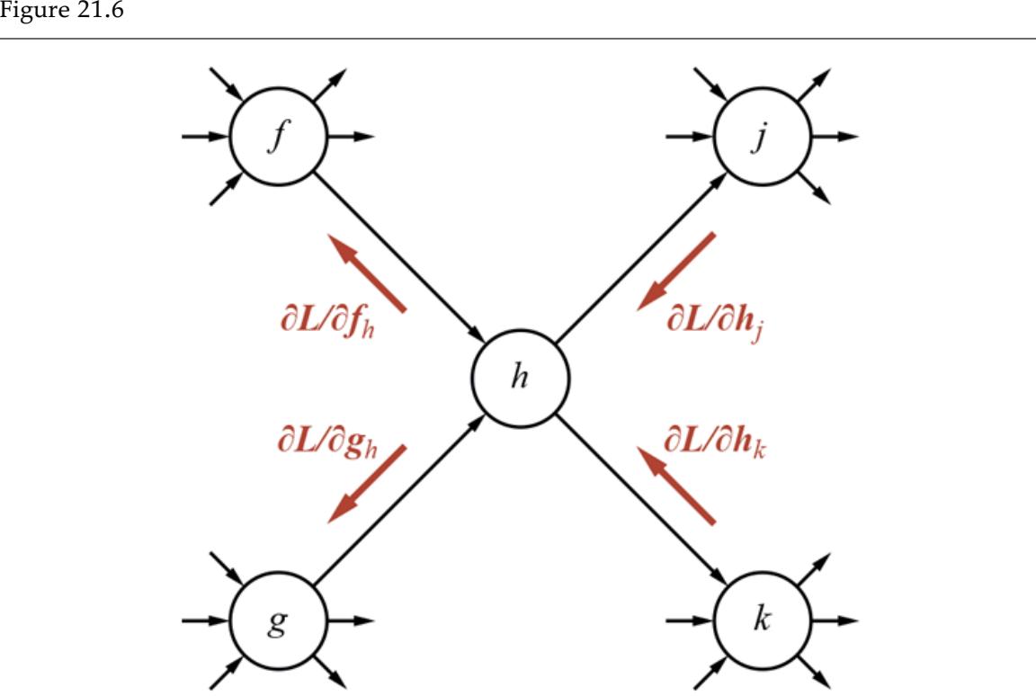
Illustration of the back-propagation of gradient information in an arbitrary computation graph. The forward computation of the output of the network proceeds from left to right, while the back-propagation of gradients proceeds from right to left.

The back-propagation process passes messages back along each link in the network. At each node, the incoming messages are collected and new messages are calculated to pass back to the next layer. As the figure shows, the messages are all partial derivatives of the loss . For example, the backward message is the partial derivative of with respect to ’s first input, which is the forward message from to . Now, affects through both and , so we have

(21.11)

\[ \partial L/\partial h = \partial L/\partial h\_j + \partial L/\partial h\_k, \]

With this equation, the node can compute the derivative of with respect to by summing the incoming messages from and . Now, to compute the outgoing messages and , we use the following equations:

(21.12)

\[\frac{\partial L}{\partial f\_h} = \frac{\partial L}{\partial h} \frac{\partial h}{\partial f\_h} \qquad \text{and} \qquad \frac{\partial L}{\partial g\_h} = \frac{\partial L}{\partial h} \frac{\partial h}{\partial g\_h}.\]

In Equation (21.12) , was already computed by Equation (21.11) , and and are just the derivatives of with respect to its first and second arguments, respectively. For example, if is a multiplication node—that is, —then and . Software packages for deep learning typically come with a library of node types (addition, multiplication, sigmoid, and so on), each of which knows how to compute its own derivatives as needed for Equation (21.12) .

The back-propagation process begins with the output nodes, where each initial message is calculated directly from the expression for in terms of the predicted value and the true value from the training data. At each internal node, the incoming backward messages are summed according to Equation (21.11) and the outgoing messages are generated from Equation (21.12) . The process terminates at each node in the computation graph that represents a weight (e.g., the light mauve ovals in Figure 21.3(b) ). At that point, the sum of the incoming messages to is —precisely the gradient we need to update . Exercise 21.BPRE asks you to apply this process to the simple network in Figure 21.3 in order to rederive the gradient expressions in Equations (21.4) and (21.5) .

Weight-sharing, as used in convolutional networks (Section 21.3 ) and recurrent networks (Section 21.6 ), is handled simply by treating each shared weight as a single node with multiple outgoing arcs in the computation graph. During back-propagation, this results in multiple incoming gradient messages. By Equation (21.11) , this means that the gradient for the shared weight is the sum of the gradient contributions from each place it is used in the network.

It is clear from this description of the back-propagation process that its computational cost is linear in the number of nodes in the computation graph, just like the cost of the forward computation. Furthermore, because the node types are typically fixed when the network is designed, all of the gradient computations can be prepared in symbolic form in advance and compiled into very efficient code for each node in the graph. Note also that the messages in Figure 21.6 need not be scalars: they could equally be vectors, matrices, or higherdimensional tensors, so that the gradient computations can be mapped onto GPUs or TPUs to benefit from parallelism.

One drawback of back-propagation is that it requires storing most of the intermediate values that were computed during forward propagation in order to calculate gradients in the backward pass. This means that the total memory cost of training the network is proportional to the number of units in the entire network. Thus, even if the network itself is represented only implicitly by propagation code with lots of loops, rather than explicitly by a data structure, all of the intermediate results of that propagation code have to be stored explicitly.

21.4.2 Batch normalization

Batch normalization is a commonly used technique that improves the rate of convergence of SGD by rescaling the values generated at the internal layers of the network from the examples within each minibatch. Although the reasons for its effectiveness are not well understood at the time of writing, we include it because it confers significant benefits in practice. To some extent, batch normalization seems to have effects similar to those of the residual network.

Batch normalization

Consider a node somewhere in the network: the values of for the examples in a minibatch are . Batch normalization replaces each with a new quantity :

\[ \hat{z}\_i = \gamma \frac{z\_i - \mu}{\sqrt{\epsilon + \sigma^2}} + \beta, \]

where is the mean value of across the minibatch, is the standard deviation of , is a small constant added to prevent division by zero, and and are learned parameters.

Batch normalization standardizes the mean and variance of the values, as determined by the values of and . This makes it much simpler to train a deep network. Without batch

normalization, information can get lost if a layer’s weights are too small, and the standard deviation at that layer decays to near zero. Batch normalization prevents this from happening. It also reduces the need for careful initialization of all the weights in the network to make sure that the nodes in each layer are in the right operating region to allow information to propagate.

With batch normalization, we usually include and , which may be node-specific or layerspecific, among the parameters of the network, so that they are included in the learning process. After training, and are fixed at their learned values.

21.5 Generalization

So far we have described how to fit a neural network to its training set, but in machine learning the goal is to generalize to new data that has not been seen previously, as measured by performance on a test set. In this section, we focus on three approaches to improving generalization performance: choosing the right network architecture, penalizing large weights, and randomly perturbing the values passing through the network during training.

21.5.1 Choosing a network architecture

A great deal of effort in deep learning research has gone into finding network architectures that generalize well. Indeed, for each particular kind of data—images, speech, text, video, and so on—a good deal of the progress in performance has come from exploring different kinds of network architectures and varying the number of layers, their connectivity, and the types of node in each layer. 6

6 Noting that much of this incremental, exploratory work is carried out by graduate students, some have called the process graduate student descent (GSD).

Some neural network architectures are explicitly designed to generalize well on particular types of data: convolutional networks encode the idea that the same feature extractor is useful at all locations across a spatial grid, and recurrent networks encode the idea that the same update rule is useful at all points in a stream of sequential data. To the extent that these assumptions are valid, we expect convolutional architectures to generalize well on images and recurrent networks to generalize well on text and audio signals.

One of the most important empirical findings in the field of deep learning is that when comparing two networks with similar numbers of weights, the deeper network usually gives better generalization performance. Figure 21.7 shows this effect for at least one real-world application—recognizing house numbers. The results show that for any fixed number of parameters, an eleven-layer network gives much lower test-set error than a three-layer network.

Deep learning systems perform well on some but not all tasks. For tasks with highdimensional inputs—images, video, speech signals, etc.—they perform better than any other pure machine learning approaches. Most of the algorithms described in Chapter 19 can handle high-dimensional input only if it is preprocessed using manually designed features to reduce the dimensionality. This preprocessing approach, which prevailed prior to 2010, has not yielded performance comparable to that achieved by deep learning systems.

Clearly, deep learning models are capturing some important aspects of these tasks. In particular, their success implies that the tasks can be solved by parallel programs with a relatively small number of steps ( to rather than, say, ). This is perhaps not surprising, because these tasks are typically solved by the brain in less than a second, which is time enough for only a few tens of sequential neuron firings. Moreover, by examining the internal-layer representations learned by deep convolutional networks for vision tasks, we find evidence that the processing steps seem to involve extracting a sequence of increasingly abstract representations of the scene, beginning with tiny edges, dots, and corner features and ending with entire objects and arrangements of multiple objects.

On the other hand, because they are simple circuits, deep learning models lack the compositional and quantificational expressive power that we see in first-order logic (Chapter 8 ) and context-free grammars (Chapter 23 ).

Although deep learning models generalize well in many cases, they may also produce unintuitive errors. They tend to produce input–output mappings that are discontinuous, so that a small change to an input can cause a large change in the output. For example, it may be possible to alter just a few pixels in an image of a dog and cause the network to classify the dog as an ostrich or a school bus—even though the altered image still looks exactly like a dog. An altered image of this kind is called an adversarial example.

Adversarial example

In low-dimensional spaces it is hard to find adversarial examples. But for an image with a million pixel values, it is often the case that even though most of the pixels contribute to the image being classified in the middle of the “dog” region of the space, there are a few dimensions where the pixel value is near the boundary to another category. An adversary with the ability to reverse engineer the network can find the smallest vector difference that would move the image over the border.

When adversarial examples were first discovered, they set off two worldwide scrambles: one to find learning algorithms and network architectures that would not be susceptible to adversarial attack, and another to create ever-more-effective adversarial attacks against all kinds of learning systems. So far the attackers seem to be ahead. In fact, whereas it was assumed initially that one would need access to the internals of the trained network in order to construct an adversarial example specifically for that network, it has turned out that one can construct robust adversarial examples that fool multiple networks with different architectures, hyperparameters, and training sets. These findings suggest that deep learning models recognize objects in ways that are quite different from the human visual system.

21.5.2 Neural architecture search

Unfortunately, we don’t yet have a clear set of guidelines to help you choose the best network architecture for a particular problem. Success in deploying a deep learning solution requires experience and good judgment.

From the earliest days of neural network research, attempts have been made to automate the process of architecture selection. We can think of this as a case of hyperparameter tuning (Section 19.4.4 ), where the hyperparameters determine the depth, width, connectivity, and other attributes of the network. However, there are so many choices to be made that simple approaches like grid search can’t cover all possibilities in a reasonable amount of time.

Neural architecture search

Therefore, it is common to use neural architecture search to explore the state space of possible network architectures. Many of the search techniques and learning techniques we covered earlier in the book have been applied to neural architecture search.

Evolutionary algorithms have been popular because it is sensible to do both recombination (joining parts of two networks together) and mutation (adding or removing a layer or changing a parameter value). Hill climbing can also be used with these same mutation operations. Some researchers have framed the problem as reinforcement learning, and some as Bayesian optimization. Another possibility is to treat the architectural possibilities as a continuous differentiable space and use gradient descent to find a locally optimal solution.

For all these search techniques, a major challenge is estimating the value of a candidate network. The straightforward way to evaluate an architecture is to train it on a test set for multiple batches and then evaluate its accuracy on a validation set. But with large networks that could take many GPU-days.

Therefore, there have been many attempts to speed up this estimation process by eliminating or at least reducing the expensive training process. We can train on a smaller data set. We can train for a small number of batches and predict how the network would improve with more batches. We can use a reduced version of the network architecture that we hope retains the properties of the full version. We can train one big network and then search for subgraphs of the network that perform better; this search can be fast because the subgraphs share parameters and don’t have to be retrained.

Another approach is to learn a heuristic evaluation function (as was done for A* search). That is, start by choosing a few hundred network architectures and train and evaluate them. That gives us a data set of (network, score) pairs. Then learn a mapping from the features of a network to a predicted score. From that point on we can generate a large number of candidate networks and quickly estimate their value. After a search through the space of networks, the best one(s) can be fully evaluated with a complete training procedure.

21.5.3 Weight decay

In Section 19.4.3 we saw that regularization—limiting the complexity of a model—can aid generalization. This is true for deep learning models as well. In the context of neural networks we usually call this approach weight decay.

Weight decay

Weight decay consists of adding a penalty to the loss function used to train the neural network, where is a hyperparameter controlling the strength of the penalty and the sum is usually taken over all of the weights in the network. Using is equivalent to not using weight decay, while using larger values of encourages the weights to become small. It is common to use weight decay with near .

Choosing a specific network architecture can be seen as an absolute constraint on the hypothesis space: a function is either representable within that architecture or it is not. Loss function penalty terms such as weight decay offer a softer constraint: functions represented with large weights are in the function family, but the training set must provide more evidence in favor of these functions than is required to choose a function with small weights.

It is not straightforward to interpret the effect of weight decay in a neural network. In networks with sigmoid activation functions, it is hypothesized that weight decay helps to keep the activations near the linear part of the sigmoid, avoiding the flat operating region that leads to vanishing gradients. With ReLU activation functions, weight decay seems to be beneficial, but the explanation that makes sense for sigmoids no longer applies because the ReLU’s output is either linear or zero. Moreover, with residual connections, weight decay encourages the network to have small differences between consecutive layers rather than small absolute weight values. Despite these differences in the behavior of weight decay across many architectures, weight decay is still widely useful.

One explanation for the beneficial effect of weight decay is that it implements a form of maximum a posteriori (MAP) learning (see page 723). Letting and stand for the inputs and outputs across the entire training set, the maximum a posteriori hypothesis satisfies

\[\begin{aligned} h\_{\text{MAP}} &= \underset{\mathbf{w}}{\text{argmax}} \, P(\mathbf{y}|\mathbf{X}, \mathbf{W})P(\mathbf{W})\\ &= \underset{\mathbf{w}}{\text{argmin}} [-\log P(\mathbf{y}|\mathbf{X}, \mathbf{W}) - \log P(\mathbf{W})]. \end{aligned}\]

The first term is the usual cross-entropy loss; the second term prefers weights that are likely under a prior distribution. This aligns exactly with a regularized loss function if we set

\[\log P(\mathbf{W}) = -\lambda \sum\_{i,j} W\_{i,j}^2,\]

which means that is a zero-mean Gaussian prior.

21.5.4 Dropout

Another way that we can intervene to reduce the test-set error of a network—at the cost of making it harder to fit the training set—is to use dropout. At each step of training, dropout applies one step of back-propagation learning to a new version of the network that is created by deactivating a randomly chosen subset of the units. This is a rough and very lowcost approximation to training a large ensemble of different networks (see Section 19.8 ).

Dropout

More specifically, let us suppose we are using stochastic gradient descent with minibatch size . For each minibatch, the dropout algorithm applies the following process to every node in the network: with probability , the unit output is multiplied by a factor of ; otherwise, the unit output is fixed at zero. Dropout is typically applied to units in the hidden layers with ; for input units, a value of turns out to be most effective. This process produces a thinned network with about half as many units as the original, to which back-propagation is applied with the minibatch of training examples. The process repeats in the usual way until training is complete. At test time, the model is run with no dropout.

We can think of dropout from several perspectives:

• By introducing noise at training time, the model is forced to become robust to noise.
• As noted above, dropout approximates the creation of a large ensemble of thinned networks. This claim can be verified analytically for linear models, and appears to hold experimentally for deep learning models.
• Hidden units trained with dropout must learn not only to be useful hidden units; they must also learn to be compatible with many other possible sets of other hidden units that may or may not be included in the full model. This is similar to the selection processes that guide the evolution of genes: each gene must not only be effective in its own function, but must work well with other genes, whose identity in future organisms may vary considerably.

Dropout applied to later layers in a deep network forces the final decision to be made robustly by paying attention to all of the abstract features of the example rather than focusing on just one and ignoring the others. For example, a classifier for animal images might be able to achieve high performance on the training set just by looking at the animal’s nose, but would presumably fail on a test case where the nose was obscured or damaged. With dropout, there will be training cases where the internal “nose unit” is zeroed out, causing the learning process to find additional identifying features. Notice that trying to achieve the same degree of robustness by adding noise to the input data would be difficult: there is no easy way to know in advance that the network is going to focus on noses, and no easy way to delete noses automatically from each image.

Altogether, dropout forces the model to learn multiple, robust explanations for each input. This causes the model to generalize well, but also makes it more difficult to fit the training set—it is usually necessary to use a larger model and to train it for more iterations.

21.6 Recurrent Neural Networks

Recurrent neural networks (RNNs) are distinct from feedforward networks in that they allow cycles in the computation graph. In all the cases we will consider, each cycle has a delay, so that units may take as input a value computed from their own output at an earlier step in the computation. (Without the delay, a cyclic circuit may reach an inconsistent state.) This allows the RNN to have internal state, or memory: inputs received at earlier time steps affect the RNN’s response to the current input.

Memory

RNNs can also be used to perform more general computations—after all, ordinary computers are just Boolean circuits with memory—and to model real neural systems, many of which contain cyclic connections. Here we focus on the use of RNNs to analyze sequential data, where we assume that a new input vector arrives at each time step.

As tools for analyzing sequential data, RNNs can be compared to the hidden Markov models, dynamic Bayesian networks, and Kalman filters described in Chapter 14 . (The reader may find it helpful to refer back to that chapter before proceeding.) Like those models, RNNs make a Markov assumption (see page 463): the hidden state of the network suffices to capture the information from all previous inputs. Furthermore, suppose we describe the RNN’s update process for the hidden state by the equation for some parameterized function . Once trained, this function represents a timehomogeneous process (page 463)—effectively a universally quantified assertion that the dynamics represented by hold for all time steps. Thus, RNNs add expressive power compared to feedforward networks, just as convolutional networks do, and just as dynamic Bayes nets add expressive power compared to regular Bayes nets. Indeed, if you tried to use a feedforward network to analyze sequential data, the fixed size of the input layer would force the network to examine only a finite-length window of data, in which case the network would fail to detect long-distance dependencies.

21.6.1 Training a basic RNN

The basic model we will consider has an input layer , a hidden layer with recurrent connections, and an output layer , as shown in Figure 21.8(a) . We assume that both and are observed in the training data at each time step. The equations defining the model refer to the values of the variables indexed by time step :

(21.13)

\[\begin{aligned} \mathbf{z}\_t &= f\_\mathbf{w}(\mathbf{z}\_{t-1}, \mathbf{x}\_t) = \mathbf{g}\_z(\mathbf{W}\_{z,z}\mathbf{z}\_{t-1} + \mathbf{W}\_{x,z}\mathbf{x}\_t) \equiv \mathbf{g}\_z(\mathbf{in}\_{z,t}),\\ \hat{\mathbf{y}}\_t &= \mathbf{g}\_u(\mathbf{W}\_{z,y}\mathbf{z}\_t) \equiv \mathbf{g}\_u(\mathbf{in}\_{y,t}), \end{aligned}\]

1. Schematic diagram of a basic RNN where the hidden layer has recurrent connections; the symbol indicates a delay. (b) The same network unrolled over three time steps to create a feedforward network. Note that the weights are shared across all time steps.

where and denote the activation functions for the hidden and output layers, respectively. As usual, we assume an extra dummy input fixed at for each unit as well as bias weights associated with those inputs.

Given a sequence of input vectors and observed outputs , we can turn this model into a feedforward network by “unrolling” it for steps, as shown in Figure 21.8(b) . Notice that the weight matrices , , and are shared across all time steps. In the unrolled network, it is easy to see that we can calculate gradients to train the weights in the usual way; the only difference is that the sharing of weights across layers makes the gradient computation a little more complicated.

To keep the equations simple, we will show the gradient calculation for an RNN with just one input unit, one hidden unit, and one output unit. For this case, making the bias weights explicit, we have and . As in Equations (21.4) and (21.5) , we will assume a squared-error loss —in this case, summed over the time steps. The derivations for the input-layer and output-layer weights and are essentially identical to Equation (21.4) , so we leave them as an exercise. For the hiddenlayer weight , the first few steps also follow the same pattern as Equation (21.4) :

(21.14)

\[\begin{split} \frac{\partial L}{\partial w\_{z,z}} &= \frac{\partial}{\partial w\_{z,z}} \sum\_{t=1}^{T} (y\_t - \hat{y}\_t)^2 = \sum\_{t=1}^{T} -2(y\_t - \hat{y}\_t) \frac{\partial \hat{y}\_t}{\partial w\_{z,z}} \\ &= \sum\_{t=1}^{T} -2(y\_t - \hat{y}\_t) \frac{\partial}{\partial w\_{z,z}} g\_y(in\_{y,t}) = \sum\_{t=1}^{T} -2(y\_t - \hat{y}\_t) g'\_y(in\_{y,t}) \frac{\partial}{\partial w\_{z,z}} in\_{y,t} \\ &= \sum\_{t=1}^{T} -2(y\_t - \hat{y}\_t) g'\_y(in\_{y,t}) \frac{\partial}{\partial w\_{z,z}} \{w\_{z,y} z\_t + w\_{0,y}\} \\ &= \sum\_{t=1}^{T} -2(y\_t - \hat{y}\_t) g'\_y(in\_{y,t}) w\_{z,y} \frac{\partial z\_t}{\partial w\_{z,z}} .\end{split}\]

Now the gradient for the hidden unit can be obtained from the previous time step as follows:

(21.15)

\[\begin{split} \frac{\partial z\_{t}}{\partial w\_{z,z}} &= \frac{\partial}{\partial w\_{z,z}} g\_{z}(in\_{z,t}) = g'\_{z}(in\_{z,t}) \frac{\partial}{\partial w\_{z,z}} in\_{z,t} = g'\_{z}(in\_{z,t}) \frac{\partial}{\partial w\_{z,z}} \{w\_{z,z}z\_{t-1} + w\_{x,z}x\_{t} + w\_{0,z}\} \\ &= g'\_{z}(in\_{z,t}) \left(z\_{t-1} + w\_{z,z}\frac{\partial z\_{t-1}}{\partial w\_{z,z}}\right), \end{split}\]

where the last line uses the rule for derivatives of products: .

Looking at Equation (21.15) , we notice two things. First, the gradient expression is recursive: the contribution to the gradient from time step is calculated using the contribution from time step . If we order the calculations in the right way, the total run time for computing the gradient will be linear in the size of the network. This algorithm is called back-propagation through time, and is usually handled automatically by deep learning software systems. Second, if we iterate the recursive calculation, we see that gradients at will include terms proportional to . For sigmoids, tanhs, and ReLUs, , so our simple RNN will certainly suffer from the vanishing gradient problem

(see page 756) if . On the other hand, if , we may experience the exploding gradient problem. (For the general case, these outcomes depend on the first eigenvalue of the weight matrix .) The next section describes a more elaborate RNN design intended to mitigate this issue.

Back-propagation through time

Exploding gradient

21.6.2 Long short-term memory RNNs

Several specialized RNN architectures have been designed with the goal of enabling information to be preserved over many time steps. One of the most popular is the long short-term memory or LSTM. The long-term memory component of an LSTM, called the memory cell and denoted by , is essentially copied from time step to time step. (In contrast, the basic RNN multiplies its memory by a weight matrix at every time step, as shown in Equation (21.13) .) New information enters the memory by adding updates; in this way, the gradient expressions do not accumulate multiplicatively over time. LSTMs also include gating units, which are vectors that control the flow of information in the LSTM via elementwise multiplication of the corresponding information vector:

The forget gate determines if each element of the memory cell is remembered (copied to the next time step) or forgotten (reset to zero).

Forget gate

The input gate determines if each element of the memory cell is updated additively by new information from the input vector at the current time step.

Input gate

The output gate determines if each element of the memory cell is transferred to the short-term memory , which plays a similar role to the hidden state in basic RNNs.

Output gate

Long short-term memory

Memory cell

Gating unit

Whereas the word “gate” in circuit design usually connotes a Boolean function, gates in LSTMs are soft—for example, elements of the memory cell vector will be partially forgotten if the corresponding elements of the forget-gate vector are small but not zero. The values for the gating units are always in the range and are obtained as the outputs of a sigmoid function applied to the current input and the previous hidden state. In detail, the update equations for the LSTM are as follows:

\[\begin{aligned} \mathbf{f}\_t &= \sigma(\mathbf{W}\_{x,f}\mathbf{x}\_t + \mathbf{W}\_{z,f}\mathbf{z}\_{t-1}) \\ \mathbf{i}\_t &= \sigma(\mathbf{W}\_{x,i}\mathbf{x}\_t + \mathbf{W}\_{z,i}\mathbf{z}\_{t-1}) \\ \mathbf{o}\_t &= \sigma(\mathbf{W}\_{x,o}\mathbf{x}\_t + \mathbf{W}\_{z,o}\mathbf{z}\_{t-1}) \\ \mathbf{c}\_t &= \mathbf{c}\_{t-1} \odot \mathbf{f}\_t + \mathbf{i}\_t \odot \tanh(\mathbf{W}\_{x,c}\mathbf{x}\_t + \mathbf{W}\_{z,c}\mathbf{z}\_{t-1}) \\ \mathbf{z}\_t &= \tanh(\mathbf{c}\_t) \odot \mathbf{o}\_t, \end{aligned}\]

where the subscripts on the various weight matrices indicate the origin and destination of the corresponding links. The symbol denotes elementwise multiplication.

LSTMs were among the first practically usable forms of RNN. They have demonstrated excellent performance on a wide range of tasks including speech recognition and handwriting recognition. Their use in natural language processing is discussed in Chapter 24 .

21.7 Unsupervised Learning and Transfer Learning

The deep learning systems we have discussed so far are based on supervised learning, which requires each training example to be labeled with a value for the target function. Although such systems can reach a high level of test-set accuracy—as shown by the ImageNet competition results, for example—they often require far more labeled data than a human would for the same task. For example, a child needs to see only one picture of a giraffe, rather than thousands, in order to be able to recognize giraffes reliably in a wide range of settings and views. Clearly, something is missing in our deep learning story; indeed, it may be the case that our current approach to supervised deep learning renders some tasks completely unattainable because the requirements for labeled data would exceed what the human race (or the universe) can supply. Moreover, even in cases where the task is feasible, labeling large data sets usually requires scarce and expensive human labor.

For these reasons, there is intense interest in several learning paradigms that reduce the dependence on labeled data. As we saw in Chapter 19 , these paradigms include unsupervised learning, transfer learning, and semisupervised learning. Unsupervised learning algorithms learn solely from unlabeled inputs , which are often more abundantly available than labeled examples. Unsupervised learning algorithms typically produce generative models, which can produce realistic text, images, audio, and video, rather than simply predicting labels for such data. Transfer learning algorithms require some labeled examples but are able to improve their performance further by studying labeled examples for different tasks, thus making it possible to draw on more existing sources of data. Semisupervised learning algorithms require some labeled examples but are able to improve their performance further by also studying unlabeled examples. This section covers deep learning approaches to unsupervised and transfer learning; while semisupervised learning is also an active area of research in the deep learning community, the techniques developed so far have not proven broadly effective in practice, so we do not cover them.

21.7.1 Unsupervised learning

Supervised learning algorithms all have essentially the same goal: given a training set of inputs and corresponding outputs , learn a function that approximates well. Unsupervised learning algorithms, on the other hand, take a training set of unlabeled

examples . Here we describe two things that such an algorithm might try to do. The first is to learn new representations—for example, new features of images that make it easier to identify the objects in an image. The second is to learn a generative model—typically in the form of a probability distribution from which new samples can be generated. (The algorithms for learning Bayes nets in Chapter 20 fall in this category.) Many algorithms are capable of both representation learning and generative modeling.

Suppose we learn a joint model , where is a set of latent, unobserved variables that represent the content of the data in some way. In keeping with the spirit of the chapter, we do not predefine the meanings of the variables; the model is free to learn to associate with however it chooses. For example, a model trained on images of handwritten digits might choose to use one direction in space to represent the thickness of pen strokes, another to represent ink color, another to represent background color, and so on. With images of faces, the learning algorithm might choose one direction to represent gender and another to capture the presence or absence of glasses, as illustrated in Figure 21.9 .

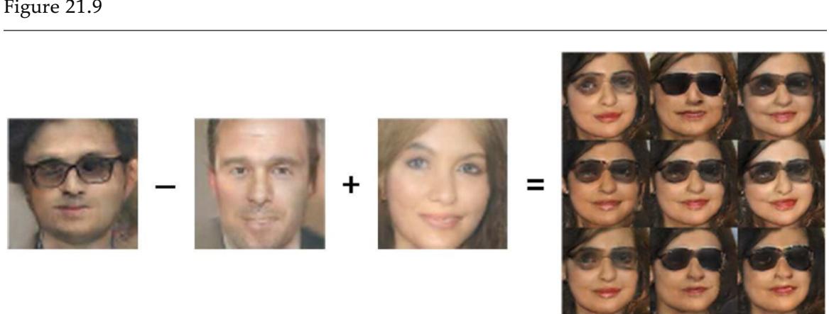
A demonstration of how a generative model has learned to use different directions in space to represent different aspects of faces. We can actually perform arithmetic in space. The images here are all generated from the learned model and show what happens when we decode different points in space. We start with the coordinates for the concept of “man with glasses,” subtract off the coordinates for “man,” add the coordinates for “woman,” and obtain the coordinates for “woman with glasses.” Images reproduced with permission from (Radford et al., 2015).

A learned probability model achieves both representation learning (it has constructed meaningful vectors from the raw vectors) and generative modeling: if we integrate out of we obtain .

Probabilistic PCA: A simple generative model

PPCA

There have been many proposals for the form that might take. One of the simplest is the probabilistic principal components analysis (PPCA) model. In a PPCA model, is chosen from a zero-mean, spherical Gaussian, then is generated from by applying a weight matrix and adding spherical Gaussian noise: 7

7 Standard PCA involves fitting a multivariate Gaussian to the raw input data and then selecting out the longest axes—the principal components—of that ellipsoidal distribution.

\[\begin{aligned} P(\mathbf{z}) &= N(\mathbf{z}; \mathbf{0}, \mathbf{I}) \\ P\_W(\mathbf{x}|\mathbf{z}) &= N(\mathbf{x}; \mathbf{W}\mathbf{z}, \sigma^2 \mathbf{I}) \end{aligned}\]

The weights (and optionally the noise parameter ) can be learned by maximizing the likelihood of the data, given by

(21.16)

\[P\_W(\mathbf{x}) = \int P\_W(\mathbf{x}, \mathbf{z})d\mathbf{z} = N(\mathbf{x}; \mathbf{0}, \mathbf{W}\mathbf{W}^\top + \sigma^2 \mathbf{I}).\]

The maximization with respect to can be done by gradient methods or by an efficient iterative EM algorithm (see Section 20.3 ). Once has been learned, new data samples can be generated directly from using Equation (21.16) . Moreover, new observations that have very low probability according to Equation (21.16) can be flagged as potential anomalies.

With PPCA, we usually assume that the dimensionality of is much less than the dimensionality of , so that the model learns to explain the data as well as possible in terms of a small number of features. These features can be extracted for use in standard classifiers by computing , the expectation of .

Generating data from a probabilistic PCA model is straightforward: first sample from its fixed Gaussian prior, then sample from a Gaussian with mean . As we will see shortly, many other generative models resemble this process, but use complicated mappings defined by deep models rather than linear mappings from -space to -space.

Autoencoders

Many unsupervised deep learning algorithms are based on the idea of an autoencoder. An autoencoder is a model containing two parts: an encoder that maps from to a representation and a decoder that maps from a representation to observed data . In general, the encoder is just a parameterized function and the decoder is just a parameterized function . The model is trained so that , so that the encoding process is roughly inverted by the decoding process. The functions and can be simple linear models parameterized by a single matrix or they can be represented by a deep neural network.

Autoencoder

A very simple autoencoder is the linear autoencoder, where both and are linear with a shared weight matrix :

\[ \begin{aligned} \hat{\mathbf{z}} &= f(\mathbf{x}) = \mathbf{W}\mathbf{x} \\ \mathbf{x} &= g(\hat{\mathbf{z}}) = \mathbf{W}^\top \hat{\mathbf{z}}. \end{aligned} \]

One way to train this model is to minimize the squared error so that . The idea is to train so that a low-dimensional will retain as much information as possible to reconstruct the high-dimensional data . This linear autoencoder turns out to be closely connected to classical principal components analysis (PCA). When is -dimensional, the matrix should learn to span the principal components of the data—in other words, the set of orthogonal directions in which the data has highest variance, or equivalently the eigenvectors of the data covariance matrix that have the largest eigenvalues—exactly as in PCA.

The PCA model is a simple generative model that corresponds to a simple linear autoencoder. The correspondence suggests that there may be a way to capture more complex kinds of generative models using more complex kinds of autoencoders. The variational autoencoder (VAE) provides one way to do this.

Variational autoencoder

Variational methods were introduced briefly on page 458 as a way to approximate the posterior distribution in complex probability models, where summing or integrating out a large number of hidden variables is intractable. The idea is to use a variational posterior , drawn from a computationally tractable family of distributions, as an approximation to the true posterior. For example, we might choose from the family of Gaussian distributions with a diagonal covariance matrix. Within the chosen family of tractable distributions, is optimized to be as close as possible to the true posterior distribution .

Variational posterior

For our purposes, the notion of “as close as possible” is defined by the KL divergence, which we mentioned on page 758. This is given by

\[D\_{KL}(Q(\mathbf{z}) \parallel P(\mathbf{z}|\mathbf{x})) = \int Q(\mathbf{z}) \log \frac{Q(\mathbf{z})}{P(\mathbf{z}|\mathbf{x})} d\mathbf{z}\]

which is an average (with respect to ) of the log ratio between and . It is easy to see that , with equality when and coincide. We can then define the variational lower bound (sometimes called the evidence lower bound, or ELBO) on the log likelihood of the data:

\[L(\mathbf{x}, Q) = \log P(\mathbf{x}) - D\_{KL}(Q(\mathbf{z}) \parallel P(\mathbf{z}|\mathbf{x})).\]

Variational lower bound

ELBO

We can see that is a lower bound for because the KL divergence is nonnegative. Variational learning maximizes with respect to parameters rather than maximizing , in the hope that the solution found, , is close to maximizing as well.

As written, does not yet seem to be any easier to maximize than . Fortunately, we can rewrite Equation (21.17) to reveal improved computational tractability:

\[\begin{aligned} L &=& \log P(\mathbf{x}) - \int Q(\mathbf{z}) \log \frac{Q(\mathbf{z})}{P(\mathbf{z}|\mathbf{x})} d\mathbf{z} \\ &=& - \int Q(\mathbf{z}) \log Q(\mathbf{z}) d\mathbf{z} + \int Q(\mathbf{z}) \log P(\mathbf{x}) P(\mathbf{z}|\mathbf{x}) d\mathbf{z} \\ &=& H(Q) + \mathbf{E}\_{\mathbf{z} \sim Q} \log P(\mathbf{z}, \mathbf{x}) \end{aligned}\]

where is the entropy of the distribution. For some variational families (such as Gaussian distributions), can be evaluated analytically. Moreover, the expectation, , admits an efficient unbiased estimate via samples of from . For each sample, can usually be evaluated efficiently—for example, if is a Bayes net, is just a product of conditional probabilities because and comprise all the variables.

Variational autoencoders provide a means of performing variational learning in the deep learning setting. Variational learning involves maximizing with respect to the parameters of both and . For a variational autoencoder, the decoder is interpreted as defining . For example, the output of the decoder might define the mean of a conditional Gaussian. Similarly, the output of the encoder is interpreted as defining the parameters of —for example, might be a Gaussian with mean . Training the variational autoencoder then consists of maximizing with respect to the parameters of both the

encoder and the decoder , which can themselves be arbitrarily complicated deep networks.

Deep autoregressive models

An autoregressive model (or AR model) is one in which each element of the data vector is predicted based on other elements of the vector. Such a model has no latent variables. If is of fixed size, an AR model can be thought of as a fully observable and possibly fully connected Bayes net. This means that calculating the likelihood of a given data vector according to an AR model is trivial; the same holds for predicting the value of a single missing variable given all the others, and for sampling a data vector from the model.

Autoregressive model

The most common application of autoregressive models is in the analysis of time series data, where an AR model of order predicts given . In the terminology of Chapter 14 , an AR model is a non-hidden Markov model. In the terminology of Chapter 23 , an gram model of letter or word sequences is an AR model of order .

In classical AR models, where the variables are real-valued, the conditional distribution is a linear–Gaussian model with fixed variance whose mean is a weighted linear combination of —in other words, a standard linear regression model. The maximum likelihood solution is given by the Yule–Walker equations, which are closely related to the normal equations on page 680.

Yule–Walker equations

A deep autoregressive model is one in which the linear–Gaussian model is replaced by an arbitrary deep network with a suitable output layer depending on whether is discrete or continuous. Recent applications of this autoregressive approach include DeepMind’s

WaveNet model for speech generation (van den Oord et al., 2016a). WaveNet is trained on raw acoustic signals, sampled 16,000 times per second, and implements a nonlinear AR model of order 4800 with a multilayer convolutional structure. In tests it proves to be substantially more realistic than previous state-of-the-art speech generation systems.

Deep autoregressive model

Generative adversarial networks

A generative adversarial network (GAN) is actually a pair of networks that combine to form a generative system. One of the networks, the generator, maps values from to in order to produce samples from the distribution . A typical scheme samples from a unit Gaussian of moderate dimension and then passes it through a deep network to obtain . The other network, the discriminator, is a classifier trained to classify inputs as real (drawn from the training set) or fake (created by the generator). GANs are a kind of implicit model in the sense that samples can be generated but their probabilities are not readily available; in a Bayes net, on the other hand, the probability of a sample is just the product of the conditional probabilities along the sample generation path.

Generative adversarial network (GAN)

Generator

Discriminator

Implicit model

The generator is closely related to the decoder from the variational autoencoder framework. The challenge in implicit modeling is to design a loss function that makes it possible to train the model using samples from the distribution, rather than maximizing the likelihood assigned to training examples from the data set.

Both the generator and the discriminator are trained simultaneously, with the generator learning to fool the discriminator and the discriminator learning to accurately separate real from fake data. The competition between generator and discriminator can be described in the language of game theory (see Chapter 18 ). The idea is that in the equilibrium state of the game, the generator should reproduce the training distribution perfectly, such that the discriminator cannot perform better than random guessing. GANs have worked particularly well for image generation tasks. For example, GANs can create photorealistic, highresolution images of people who have never existed (Karras et al., 2017).

Unsupervised translation

Translation tasks, broadly construed, consist of transforming an input that has rich structure into an output that also has rich structure. In this context, “rich structure” means that the data are multidimensional and have interesting statistical dependencies among the various dimensions. Images and natural language sentences have a rich structure, but a single number, such as a class ID, does not. Transforming a sentence from English to French or converting a photo of a night scene into an equivalent photo taken during the daytime are both examples of translation tasks.

Supervised translation consists of gathering many pairs and training the model to map each to the corresponding . For example, machine translation systems are often trained on pairs of sentences that have been translated by professional human translators. For other kinds of translation, supervised training data may not be available. For example, consider a photo of a night scene containing many moving cars and pedestrians. It is presumably not feasible to find all of the cars and pedestrians and return them to their original positions in the night-time photo in order to retake the same photo in the daytime. To overcome this difficulty, it is possible to use unsupervised translation techniques that are capable of

training on many examples of and many separate examples of but no corresponding pairs.

Unsupervised translation

These approaches are generally based on GANs; for example, one can train a GAN generator to produce a realistic example of when conditioned on , and another GAN generator to perform the reverse mapping. The GAN training framework makes it possible to train a generator to generate any one of many possible samples that the discriminator accepts as a realistic example of given , without any need for a specific paired as is traditionally needed in supervised learning. More detail on unsupervised translation for images is given in Section 25.7.5 .

21.7.2 Transfer learning and multitask learning

In transfer learning, experience with one learning task helps an agent learn better on another task. For example, a person who has already learned to play tennis will typically find it easier to learn related sports such as racquetball and squash; a pilot who has learned to fly one type of commercial passenger airplane will very quickly learn to fly another type; a student who has already learned algebra finds it easier to learn calculus.

Transfer learning

We do not yet know the mechanisms of human transfer learning. For neural networks, learning consists of adjusting weights, so the most plausible approach for transfer learning is to copy over the weights learned for task A to a network that will be trained for task B. The weights are then updated by gradient descent in the usual way using data for task B. It may be a good idea to use a smaller learning rate in task B, depending on how similar the tasks are and how much data was used in task A.

Notice that this approach requires human expertise in selecting the tasks: for example, weights learned during algebra training may not be very useful in a network intended for racquetball. Also, the notion of copying weights requires a simple mapping between the input spaces for the two tasks and essentially identical network architectures.

One reason for the popularity of transfer learning is the availability of high-quality pretrained models. For example, you could download a pretrained visual object recognition model such as the ResNet-50 model trained on the COCO data set, thereby saving yourself weeks of work. From there you can modify the model parameters by supplying additional images and object labels for your specific task.

Suppose you want to classify types of unicycles. You have only a few hundred pictures of different unicycles, but the COCO data set has over 3,000 images in each of the categories of bicycles, motorcycles, and skateboards. This means that a model pretrained on COCO already has experience with wheels and roads and other relevant features that will be helpful in interpreting the unicycle images.

Often you will want to freeze the first few layers of the pretrained model—these layers serve as feature detectors that will be useful for your new model. Your new data set will be allowed to modify the parameters of the higher levels only; these are the layers that identify problem-specific features and do classification. However, sometimes the difference between sensors means that even the lowest-level layers need to be retrained.

As another example, for those building a natural language system, it is now common to start with a pretrained model such as the ROBERTA model (see Section 24.6 ), which already “knows” a great deal about the vocabulary and syntax of everyday language. The next step is to fine-tune the model in two ways. First, by giving it examples of the specialized vocabulary used in the desired domain; perhaps a medical domain (where it will learn about “mycardial infarction”) or perhaps a financial domain (where it will learn about “fiduciary responsibility”). Second, by training the model on the task it is to perform. If it is to do question answering, train it on question/answer pairs.

One very important kind of transfer learning involves transfer between simulations and the real world. For example, the controller for a self-driving car can be trained on billions of

miles of simulated driving, which would be impossible in the real world. Then, when the controller is transitioned to the real vehicle, it adapts quickly to the new environment.

Multitask learning is a form of transfer learning in which we simultaneously train a model on multiple objectives. For example, rather than training a natural language system on partof-speech tagging and then transferring the learned weights to a new task such as document classification, we train one system simultaneously on part-of-speech tagging, document classification, language detection, word prediction, sentence difficulty modeling, plagiarism detection, sentence entailment, and question answering. The idea is that to solve any one of these tasks, a model might be able to take advantage of superficial features of the data. But to solve all eight at once with a common representation layer, the model is more likely to create a common representation that reflects real natural language usage and content.

Multitask learning

21.8 Applications

Deep learning has been applied successfully to many important problem areas in AI. For indepth explanations, we refer the reader to the relevant chapters: Chapter 22 for the use of deep learning in reinforcement learning systems, Chapter 24 for natural language processing, Chapter 25 (particularly Section 25.4 ) for computer vision, and Chapter 26 for robotics.

21.8.1 Vision

We begin with computer vision, which is the application area that has arguably had the biggest impact on deep learning, and vice versa. Although deep convolutional networks had been in use since the 1990s for tasks such as handwriting recognition, and neural networks had begun to surpass generative probability models for speech recognition by around 2010, it was the success of the AlexNet deep learning system in the 2012 ImageNet competition that propelled deep learning into the limelight.

The ImageNet competition was a supervised learning task with 1,200,000 images in 1,000 different categories, and systems were evaluated on the “top-5” score—how often the correct category appears in the top five predictions. AlexNet achieved an error rate of 15.3%, whereas the next best system had an error rate of more than 25%. AlexNet had five convolutional layers interspersed with max-pooling layers, followed by three fully connected layers. It used ReLU activation functions and took advantage of GPUs to speed up the process of training 60 million weights.

Since 2012, with improvements in network design, training methods, and computing resources, the top-5 error rate has been reduced to less than 2%—well below the error rate of a trained human (around 5%). CNNs have been applied to a wide range of vision tasks, from self-driving cars to grading cucumbers. Driving, which is covered in Section 25.7.6 and in several sections of Chapter 26 , is among the most demanding of vision tasks: not only must the algorithm detect, localize, track, and recognize pigeons, paper bags, and pedestrians, but it has to do it in real time with near-perfect accuracy. 8

8 The widely known tale of the Japanese cucumber farmer who built his own cucumber-sorting robot using TensorFlow is, it turns out, mostly mythical. The algorithm was developed by the farmer’s son, who worked previously as a software engineer at Toyota, and

21.8.2 Natural language processing

Deep learning has also had a huge impact on natural language processing (NLP) applications such as machine translation and speech recognition. Some advantages of deep learning for these applications include the possibility of end-to-end learning, the automatic generation of internal representations for the meanings of words, and the interchangeability of learned encoders and decoders.

End-to-end learning refers to the construction of entire systems as a single, learned function . For example, an for machine translation might take as input an English sentence and produce an equivalent Japanese sentence . Such an can be learned from training data in the form of human-translated pairs of sentences (or even pairs of texts, where the alignment of corresponding sentences or phrases is part of the problem to be solved). A more classical pipeline approach might first parse , then extract its meaning, then reexpress the meaning in Japanese as , then post-edit using a language model for Japanese. This pipeline approach has two major drawbacks: first, errors are compounded at each stage; and second, humans have to determine what constitutes a “parse tree” and a “meaning representation,” but there is no easily accessible ground truth for these notions, and our theoretical ideas about them are almost certainly incomplete.

At our present stage of understanding, then, the classical pipeline approach—which, at least naively, seems to correspond to how a human translator works—is outperformed by the end-to-end method made possible by deep learning. For example, Wu et al. (2016b) showed that end-to-end translation using deep learning reduced translation errors by 60% relative to a previous pipeline-based system. As of 2020, machine translation systems are approaching human performance for language pairs such as French and English for which very large paired data sets are available, and they are usable for other language pairs covering the majority of Earth’s population. There is even some evidence that networks trained on multiple languages do in fact learn an internal meaning representation: for example, after learning to translate Portuguese to English and English to Spanish, it is possible to translate Portuguese directly into Spanish without any Portuguese/Spanish sentence pairs in the training set.

One of the most significant findings to emerge from the application of deep learning to language tasks is that a great deal deal of mileage comes from re-representing individual words as vectors in a high-dimensional space—so-called word embeddings (see Section 24.1 ). The vectors are usually extracted from the weights of the first hidden layer of a network trained on large quantities of text, and they capture the statistics of the lexical contexts in which words are used. Because words with similar meanings are used in similar contexts, they end up close to each other in the vector space. This allows the network to generalize effectively across categories of words, without the need for humans to predefine those categories. For example, a sentence beginning “John bought a watermelon and two pounds of …” is likely to continue with “apples” or “bananas” but not with “thorium” or “geography.” Such a prediction is much easier to make if “apples” and “bananas” have similar representations in the internal layer.

21.8.3 Reinforcement learning

In reinforcement learning (RL), a decision-making agent learns from a sequence of reward signals that provide some indication of the quality of its behavior. The goal is to optimize the sum of future rewards. This can be done in several ways: in the terminology of Chapter 17 , the agent can learn a value function, a Q-function, a policy, and so on. From the point of view of deep learning, all these are functions that can be represented by computation graphs. For example, a value function in Go takes a board position as input and returns an estimate of how advantageous the position is for the agent. While the methods of training in RL differ from those of supervised learning, the ability of multilayer computation graphs to represent complex functions over large input spaces has proved to be very useful. The resulting field of research is called deep reinforcement learning.

Deep reinforcement learning

In the 1950s, Arthur Samuel experimented with multilayer representations of value functions in his work on reinforcement learning for checkers, but he found that in practice a linear function approximator worked best. (This may have been a consequence of working with a computer roughly 100 billion times less powerful than a modern tensor processing unit.) The first major successful demonstration of deep RL was DeepMind’s Atari-playing

agent, DQN (Mnih et al., 2013). Different copies of this agent were trained to play each of several different Atari video games, and demonstrated skills such as shooting alien spaceships, bouncing balls with paddles, and driving simulated racing cars. In each case, the agent learned a Q-function from raw image data with the reward signal being the game score. Subsequent work has produced deep RL systems that play at a superhuman level on the majority of the 57 different Atari games. DeepMind’s ALPHAGO system also used deep RL to defeat the best human players at the game of Go (see Chapter 5 ).

Despite its impressive successes, deep RL still faces significant obstacles: it is often difficult to get good performance, and the trained system may behave very unpredictably if the environment differs even a little from the training data (Irpan, 2018). Compared to other applications of deep learning, deep RL is rarely applied in commercial settings. It is, nonetheless, a very active area of research.

Summary

This chapter described methods for learning functions represented by deep computational graphs. The main points were:

• Neural networks represent complex nonlinear functions with a network of parameterized linear-threshold units.
• The back-propagation algorithm implements a gradient descent in parameter space to minimize the loss function.
• Deep learning works well for visual object recognition, speech recognition, natural language processing, and reinforcement learning in complex environments.
• Convolutional networks are particularly well suited for image processing and other tasks where the data have a grid topology.
• Recurrent networks are effective for sequence-processing tasks including language modeling and machine translation.

Bibliographical and Historical Notes

The literature on neural networks is vast. Cowan and Sharp (1988b, 1988a) survey the early history, beginning with the work of McCulloch and Pitts (1943). (As mentioned in Chapter 1 , John McCarthy has pointed to the work of Nicolas Rashevsky (1936, 1938) as the earliest mathematical model of neural learning.) Norbert Wiener, a pioneer of cybernetics and control theory (Wiener, 1948), worked with McCulloch and Pitts and influenced a number of young researchers, including Marvin Minsky, who may have been the first to develop a working neural network in hardware, in 1951 (see Minsky and Papert, 1988, pp. ix–x). Alan Turing (1948) wrote a research report titled Intelligent Machinery that begins with the sentence “I propose to investigate the question as to whether it is possible for machinery to show intelligent behaviour” and goes on to describe a recurrent neural network architecture he called “B-type unorganized machines” and an approach to training them. Unfortunately, the report went unpublished until 1969, and was all but ignored until recently.

The perceptron, a one-layer neural network with a hard-threshold activation function, was popularized by Frank Rosenblatt (1957). After a demonstration in July 1958, the New York Times described it as “the embryo of an electronic computer that [the Navy] expects will be able to walk, talk, see, write, reproduce itself and be conscious of its existence.” Rosenblatt (1960) later proved the perceptron convergence theorem, although it had been foreshadowed by purely mathematical work outside the context of neural networks (Agmon, 1954; Motzkin and Schoenberg, 1954). Some early work was also done on multilayer networks, including Gamba perceptrons (Gamba et al., 1961) and madalines (Widrow, 1962). Learning Machines (Nilsson, 1965) covers much of this early work and more. The subsequent demise of early perceptron research efforts was hastened (or, the authors later claimed, merely explained) by the book Perceptrons (Minsky and Papert, 1969), which lamented the field’s lack of mathematical rigor. The book pointed out that single-layer perceptrons could represent only linearly separable concepts and noted the lack of effective learning algorithms for multilayer networks. These limitations were already well known (Hawkins, 1961) and had been acknowledged by Rosenblatt himself (Rosenblatt, 1962).

The papers collected by Hinton and Anderson (1981), based on a conference in San Diego in 1979, can be regarded as marking a renaissance of connectionism. The two-volume “PDP” (Parallel Distributed Processing) anthology (Rumelhart and McClelland, 1986) helped to spread the gospel, so to speak, particularly in the psychology and cognitive science communities. The most important development of this period was the back-propagation algorithm for training multilayer networks.

The back-propagation algorithm was discovered independently several times in different contexts (Kelley, 1960; Bryson, 1962; Dreyfus, 1962; Bryson and Ho, 1969; Werbos, 1974; Parker, 1985) and Stuart Dreyfus (1990) calls it the “Kelley–Bryson gradient procedure.” Although Werbos had applied it to neural networks, this idea did not become widely known until a paper by David Rumelhart, Geoff Hinton, and Ron Williams (1986) appeared in Nature giving a nonmathematical presentation of the algorithm. Mathematical respectability was enhanced by papers showing that multilayer feedforward networks are (subject to technical conditions) universal function approximators (Cybenko, 1988, Cybenko, 1989). The late 1980s and early 1990s saw a huge growth in neural network research: the number of papers mushroomed by a factor of 200 between 1980–84 and 1990–94.

In the late 1990s and early 2000s, interest in neural networks waned as other techniques such as Bayes nets, ensemble methods, and kernel machines came to the fore. Interest in deep models was sparked when Geoff Hinton’s research on deep Bayesian networks generative models with category variables at the root and evidence variables at the leaves began to bear fruit, outperforming kernel machines on small benchmark data sets (Hinton et al., 2006). Interest in deep learning exploded when Krizhevsky et al., 2013 used deep convolutional networks to win the ImageNet competition (Russakovsky et al., 2015).

Commentators often cite the availability of “big data” and the processing power of GPUs as the main contributing factors in the emergence of deep learning. Architectural improvements were also important, including the adoption of the ReLU activation function instead of the logistic sigmoid (Jarrett et al., 2009; Nair and Hinton, 2010; Glorot et al., 2011) and later the development of residual networks (He et al., 2016).

On the algorithmic side, the use of stochastic gradient descent (SGD) with small batches was essential in allowing neural networks to scale to large data sets (Bottou and Bousquet, 2008). Batch normalization (Ioffe and Szegedy, 2015) also helped in making the training process faster and more reliable and has spawned several additional normalization techniques (Ba et al., 2016; Wu and He, 2018; Miyato et al., 2018). Several papers have

studied the empirical behavior of SGD on large networks and large data sets (Dauphin et al., 2015; Choromanska et al., 2014; Goodfellow et al., 2015b). On the theoretical side, some progress has been made on explaining the observation that SGD applied to overparameterized networks often reaches a global minimum with a training error of zero, although so far the theorems to this effect assume a network with layers far wider than would ever occur in practice (Allen-Zhu et al., 2018; Du et al., 2018). Such networks have more than enough capacity to function as lookup tables for the training data.

The last piece of the puzzle, at least for vision applications, was the use of convolutional networks. These had their origins in the descriptions of the mammalian visual system by neurophysiologists David Hubel and Torsten Wiesel (Hubel and Wiesel, 1959, 1962, 1968). They described “simple cells” in the visual system of a cat that resemble edge detectors, as well as “complex cells” that are invariant to some transformations such as small spatial translations. In modern convolutional networks, the output of a convolution is analogous to a simple cell while the output of a pooling layer is analogous to a complex cell.

The work of Hubel and Wiesel inspired many of the early connectionist models of vision (Marr and Poggio, 1976). The neocognitron (Fukushima, 1980; Fukushima and Miyake, 1982), designed as a model of the visual cortex, was essentially a convolutional network in terms of model architecture, although an effective training algorithm for such networks had to wait until Yann LeCun and collaborators showed how to apply back-propagation (LeCun et al., 1995). One of the early commercial successes of neural networks was handwritten digit recognition using convolutional networks (LeCun et al., 1995).

Recurrent neural networks (RNNs) were commonly proposed as models of brain function in the 1970s, but no effective learning algorithms were associated with these proposals. The method of back-propagation through time appears in the PhD thesis of Paul Werbos (1974), and his later review paper (Werbos, 1990) gives several additional references to rediscoveries of the method in the 1980s. One of the most influential early works on RNNs was due to Jeff Elman (1990), building on an RNN architecture suggested by Michael Jordan (1986). Williams and Zipser (1989) present an algorithm for online learning in RNNs. Bengio et al., 1994 analyzed the problem of vanishing gradients in recurrent networks. The long short-term memory (LSTM) architecture (Hochreiter, 1991; Hochreiter and Schmidhuber, 1997; Gers et al., 2000) was proposed as a way of avoiding this problem. More recently, effective RNN designs have been derived automatically (Jozefowicz et al., 2015; Zoph and Le, 2016).

Many methods have been tried for improving generalization in neural networks. Weight decay was suggested by Hinton (1987) and analyzed mathematically by Krogh and Hertz (1992). The dropout method is due to Srivastava et al. (2014a). Szegedy et al., 2013 introduced the idea of adversarial examples, spawning a huge literature.

Poole et al., 2017 showed that deep networks (but not shallow ones) can disentangle complex functions into flat manifolds in the space of hidden units. Rolnick and Tegmark (2018) showed that the number of units required to approximate a certain class of polynomials of variables grows exponentially for shallow networks but only linearly for deep networks.

White et al., 2019 showed that their BANANAS system could do neural architecture search (NAS) by predicting the accuracy of a network to within 1% after training on just 200 random sample architectures. Zoph and Le (2016) use reinforcement learning to search the space of neural network architectures. Real et al., 2018 use an evolutionary algorithm to do model selection, Liu et al., 2017 use evolutionary algorithms on hierarchical representations, and Jaderberg et al., 2017 describe population-based training. Liu et al., 2019 relax the space of architectures to a continuous differentiable space and use gradient descent to find a locally optimal solution. Pham et al., 2018 describe the ENAS (Efficient Neural Architecture Search) system, which searches for optimal subgraphs of a larger graph. It is fast because it does not need to retrain parameters. The idea of searching for a subgraph goes back to the “optimal brain damage” algorithm of LeCun et al., (1990).

Despite this impressive array of approaches, there are critics who feel the field has not yet matured. Yu et al., 2019 show that in some cases these NAS algorithms are no more efficient than random architecture selection. For a survey of recent results in neural architecture search, see Elsken et al., 2018.

Unsupervised learning constitutes a large subfield within statistics, mostly under the heading of density estimation. Silverman (1986) and Murphy (2012) are good sources for classical and modern techniques in this area. Principal components analysis (PCA) dates back to Pearson (1901); the name comes from independent work by Hotelling (1933). The probabilistic PCA model (Tipping and Bishop, 1999) adds a generative model for the principal components themselves. The variational autoencoder is due to Kingma and Welling (2013) and Rezende et al., 2014; Jordan et al., 1999 provide an introduction to variational methods for inference in graphical models.

For autoregressive models, the classic text is by Box et al., 2016. The Yule–Walker equations for fitting AR models were developed independently by Yule (1927) and Walker (1931). Autoregressive models with nonlinear dependencies were developed by several authors (Frey, 1998; Bengio and Bengio, 2001; Larochelle and Murray, 2011). The autoregressive WaveNet model (van den Oord et al., 2016a) was based on earlier work on autoregressive image generation (van den Oord et al., 2016b). Generative adversarial networks, or GANs, were first proposed by Goodfellow et al. (2015a), and have found many applications in AI. Some theoretical understanding of their properties is emerging, leading to improved GAN models and algorithms (Li and Malik, 2018b, 2018a; Zhu et al., 2019). Part of that understanding involves protecting against adversarial attacks (Carlini et al., 2019).

Several branches of research into neural networks have been popular in the past but are not actively explored today. Hopfield networks (Hopfield, 1982) have symmetric connections between each pair of nodes and can learn to store patterns in an associative memory, so that an entire pattern can be retrieved by indexing into the memory using a fragment of the pattern. Hopfield networks are deterministic; they were later generalized to stochastic Boltzmann machines (Hinton and Sejnowski, 1983, 1986). Boltzmann machines are possibly the earliest example of a deep generative model. The difficulty of inference in Boltzmann machines led to advances in both Monte Carlo techniques and variational techniques (see Section 13.4 ).

Hopfield network

Boltzmann machine

Research on neural networks for AI has also been intertwined to some extent with research into biological neural networks. The two topics coincided in the 1940s, and ideas for convolutional networks and reinforcement learning can be traced to studies of biological systems; but at present, new ideas in deep learning tend to be based on purely computational or statistical concerns. The field of computational neuroscience aims to build computational models that capture important and specific properties of actual biological systems. Overviews are given by Dayan and Abbott (2001) and Trappenberg (2010).

Computational neuroscience

For modern neural nets and deep learning, the leading textbooks are those by Goodfellow et al., 2016 and Charniak (2018). There are also many hands-on guides associated with the various open-source software packages for deep learning. Three of the leaders of the field— Yann LeCun, Yoshua Bengio, and Geoff Hinton—introduced the key ideas to non-AI researchers in an influential Nature article (2015). The three were recipients of the 2018 Turing Award. Schmidhuber (2015) provides a general overview, and Deng et al., 2014 focus on signal processing tasks.

The primary publication venues for deep learning research are the conference on Neural Information Processing Systems (NeurIPS), the International Conference on Machine Learning (ICML), and the International Conference on Learning Representations (ICLR). The main journals are Machine Learning, the Journal of Machine Learning Research, and Neural Computation. Increasingly, because of the fast pace of research, papers appear first on arXiv.org and are often described in the research blogs of the major research centers.

Chapter 22 Reinforcement Learning

In which we see how experiencing rewards and punishments can teach an agent how to maximize rewards in the future.

With supervised learning, an agent learns by passively observing example input/output pairs provided by a “teacher.” In this chapter, we will see how agents can actively learn from their own experience, without a teacher, by considering their own ultimate success or failure.

22.1 Learning from Rewards

Consider the problem of learning to play chess. Let’s imagine treating this as a supervised learning problem using the methods of Chapters 19 –21 . The chess-playing agent function takes as input a board position and returns a move, so we train this function by supplying examples of chess positions, each labeled with the correct move. Now, it so happens that we have available databases of several million grandmaster games, each a sequence of positions and moves. The moves made by the winner are, with few exceptions, assumed to be good, if not always perfect. Thus, we have a promising training set. The problem is that there are relatively few examples (about ) compared to the space of all possible chess positions (about ). In a new game, one soon encounters positions that are significantly different from those in the database, and the trained agent function is likely to fail miserably—not least because it has no idea of what its moves are supposed to achieve (checkmate) or even what effect the moves have on the positions of the pieces. And of course chess is a tiny part of the real world. For more realistic problems, we would need much vaster grandmaster databases, and they simply don’t exist. 1

1 As Yann LeCun and Alyosha Efros have pointed out, “the AI revolution will not be supervised.”

An alternative is reinforcement learning (RL), in which an agent interacts with the world and periodically receives rewards (or, in the terminology of psychology, reinforcements) that reflect how well it is doing. For example, in chess the reward is for winning, for losing, and for a draw. We have already seen the concept of rewards in Chapter 17 for Markov decision processes (MDPs). Indeed, the goal is the same in reinforcement learning: maximize the expected sum of rewards. Reinforcement learning differs from “just solving an MDP” because the agent is not given the MDP as a problem to solve; the agent is in the MDP. It may not know the transition model or the reward function, and it has to act in order to learn more. Imagine playing a new game whose rules you don’t know; after a hundred or so moves, the referee tells you “You lose.” That is reinforcement learning in a nutshell.

Reinforcement learning

From our point of view as designers of AI systems, providing a reward signal to the agent is usually much easier than providing labeled examples of how to behave. First, the reward function is often (as we saw for chess) very concise and easy to specify: it requires only a few lines of code to tell the chess agent if it has won or lost the game or to tell the car-racing agent that it has won or lost the race or has crashed. Second, we don’t have to be experts, capable of supplying the correct action in any situation, as would be the case if we tried to apply supervised learning.

It turns out, however, that a little bit of expertise can go a long way in reinforcement learning. The two examples in the preceding paragraph—the win/loss rewards for chess and racing—are what we call sparse rewards, because in the vast majority of states the agent is given no informative reward signal at all. In games such as tennis and cricket, we can easily supply additional rewards for each point won or for each run scored. In car racing, we could reward the agent for making progress around the track in the right direction. When learning to crawl, any forward motion is an achievement. These intermediate rewards make learning much easier.

Sparse

As long as we can provide the correct reward signal to the agent, reinforcement learning provides a very general way to build AI systems. This is particularly true for simulated environments, where there is no shortage of opportunities to gain experience. The addition of deep learning as a tool within RL systems has also made new applications possible, including learning to play Atari video games from raw visual input (Mnih et al., 2013), controlling robots (Levine et al., 2016), and playing poker (Brown and Sandholm, 2017).

Literally hundreds of different reinforcement learning algorithms have been devised, and many of them can employ as tools a wide range of learning methods from Chapters 19 – 21 . In this chapter, we cover the basic ideas and give some sense of the variety of approaches through a few examples. We categorize the approaches as follows:

MODEL-BASED REINFORCEMENT LEARNING: In these approaches the agent uses a transition model of the environment to help interpret the reward signals and to make decisions about how to act. The model may be initially unknown, in which case the agent learns the model from observing the effects of its actions, or it may already be known—for example, a chess program may know the rules of chess even if it does not know how to choose good moves. In partially observable environments, the transition model is also useful for state estimation (see Chapter 14 ). Model-based reinforcement learning systems often learn a utility function , defined (as in Chapter 17 ) in terms of the sum of rewards from state onward. 2

2 In the RL literature, which draws more on operations research than economics, utility functions are often called value functions and denoted .

Model-based reinforcement learning

MODEL-FREE REINFORCEMENT LEARNING: In these approaches the agent neither knows nor learns a transition model for the environment. Instead, it learns a more direct representation of how to behave. This comes in one of two varieties:

Model-free reinforcement learning

ACTION-UTILITY LEARNING: We introduced action-utility functions in Chapter 17 . The most common form of action-utility learning is Q-learning, where the agent learns a Q-function, or quality-function, , denoting the sum of rewards from state onward if action is taken. Given a Q-function, the agent can choose what to do in by finding the action with the highest Q-value.

Action-utility learning

Q-learning

Q-function

POLICY SEARCH: The agent learns a policy that maps directly from states to actions. In the terminology of Chapter 2 , this a reflex agent.

Policy search

We begin in Section 22.2 with passive reinforcement learning, where the agent’s policy is fixed and the task is to learn the utilities of states (or of state–action pairs); this could also involve learning a model of the environment. (An understanding of Markov decision processes, as described in Chapter 17 , is essential for this section.) Section 22.3 covers active reinforcement learning, where the agent must also figure out what to do. The principal issue is exploration: an agent must experience as much as possible of its environment in order to learn how to behave in it. Section 22.4 discusses how an agent can use inductive learning (including deep learning methods) to learn much faster from its experiences. We also discuss other approaches that can help scale up RL to solve real problems, including providing intermediate pseudorewards to guide the learner and organizing behavior into a hierarchy of actions. Section 22.5 covers methods for policy search. In Section 22.6 , we explore apprenticeship learning: training a learning agent using demonstrations rather than reward signals. Finally, Section 22.7 reports on applications of reinforcement learning.

Passive reinforcement learning

Active reinforcement learning

22.2 Passive Reinforcement Learning

We start with the simple case of a fully observable environment with a small number of actions and states, in which an agent already has a fixed policy that determines its actions. The agent is trying to learn the utility function —the expected total discounted reward if policy is executed beginning in state . We call this a passive learning agent.

Passive learning agent

The passive learning task is similar to the policy evaluation task, part of the policy iteration algorithm described in Section 17.2.2 . The difference is that the passive learning agent does not know the transition model , which specifies the probability of reaching state from state after doing action ; nor does it know the reward function , which specifies the reward for each transition.

We will use as our example the world introduced in Chapter 17 . Figure 22.1 shows the optimal policies for that world and the corresponding utilities. The agent executes a set of trials in the environment using its policy . In each trial, the agent starts in state (1,1) and experiences a sequence of state transitions until it reaches one of the terminal states, (4,2) or (4,3). Its percepts supply both the current state and the reward received for the transition that just occurred to reach that state. Typical trials might look like this:

\[\begin{array}{c}(1,1) \xrightarrow[Up]{\bullet \mathbf{04}}(1,2) \xrightarrow[Up]{\bullet \mathbf{04}}(1,3) \xrightarrow[Rights]{\bullet \mathbf{04}}(1,2) \xrightarrow[Up]{\bullet \mathbf{04}}(1,3) \xrightarrow[Rights]{\bullet \mathbf{04}}(2,3) \xrightarrow[Rights]{\bullet \mathbf{04}}(3,3) \xrightarrow[Rights]{\bullet \mathbf{16}}(4,3) \\\ (1,1) \xrightarrow[Op]{\bullet \mathbf{04}}(1,2) \xrightarrow[Op]{\bullet \mathbf{04}}(1,3) \xrightarrow[Rights]{\bullet \mathbf{04}}(2,3) \xrightarrow[Rights]{\bullet \mathbf{04}}(3,3) \xrightarrow[Rights]{\bullet \mathbf{04}}(3,2) \xrightarrow[Up]{\bullet \mathbf{04}}(3,3) \xrightarrow[Rights]{\bullet \mathbf{16}}(4,3) \\\ (1,1) \xrightarrow[Op]{\bullet \mathbf{04}}(1,2) \xrightarrow[Rights]{\bullet \mathbf{04}}(1,3) \xrightarrow[Rights]{\bullet \mathbf{04}}(2,3) \xrightarrow[Rights]{\bullet \mathbf{04}}(3,3) \xrightarrow[Rights]{\bullet \mathbf{16}}(4,2) \\\ \end{array}\]

Figure 22.1

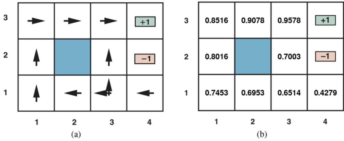
1. The optimal policies for the stochastic environment with for transitions between nonterminal states. There are two policies because in state (3,1) both and are optimal. We saw this before in Figure 17.2 . (b) The utilities of the states in the world, given policy .

Note that each transition is annotated with both the action taken and the reward received at the next state. The object is to use the information about rewards to learn the expected utility associated with each nonterminal state . The utility is defined to be the expected sum of (discounted) rewards obtained if policy is followed. As in Equation (17.2) on page 567, we write

(22.1)

\[U^{\pi}(s) = E\left[\sum\_{t=0}^{\infty} \gamma^t R(S\_t, \pi(S\_t), S\_{t+1})\right],\]

where is the reward received when action is taken in state and reaches state . Note that is a random variable denoting the state reached at time when executing policy , starting from state . We will include a discount factor in all of our equations, but for the world we will set , which means no discounting.

22.2.1 Direct utility estimation

The idea of direct utility estimation is that the utility of a state is defined as the expected total reward from that state onward (called the expected reward-to-go), and that each trial provides a sample of this quantity for each state visited. For example, the first of the three trials shown earlier provides a sample total reward of 0.76 for state (1,1), two samples of 0.80 and 0.88 for (1,2), two samples of 0.84 and 0.92 for (1,3), and so on. Thus, at the end of each sequence, the algorithm calculates the observed reward-to-go for each state and updates the estimated utility for that state accordingly, just by keeping a running average for each state in a table. In the limit of infinitely many trials, the sample average will converge to the true expectation in Equation (22.1) .

Direct utility estimation

Reward-to-go

This means that we have reduced reinforcement learning to a standard supervised learning problem in which each example is a (state, reward-to-go) pair. We have a lot of powerful algorithms for supervised learning, so this approach seems promising, but it ignores an important constraint: The utility of a state is determined by the reward and the expected utility of the successor states. More specifically, the utility values obey the Bellman equations for a fixed policy (see also Equation (17.14) ):

(22.2)

\[U\_i(s) = \sum\_{s'} P(s'|s, \pi\_i(s)) [R(s, \pi\_i(s), s') + \gamma U\_i(s')].\]

By ignoring the connections between states, direct utility estimation misses opportunities for learning. For example, the second of the three trials given earlier reaches the state (3,2), which has not previously been visited. The next transition reaches (3,3), which is known from the first trial to have a high utility. The Bellman equation suggests immediately that (3,2) is also likely to have a high utility, because it leads to (3,3), but direct utility estimation learns nothing until the end of the trial. More broadly, we can view direct utility estimation as searching for in a hypothesis space that is much larger than it needs to be, in that it includes many functions that violate the Bellman equations. For this reason, the algorithm often converges very slowly.

22.2.2 Adaptive dynamic programming

An adaptive dynamic programming (or ADP) agent takes advantage of the constraints among the utilities of states by learning the transition model that connects them and solving the corresponding Markov decision process using dynamic programming. For a passive learning agent, this means plugging the learned transition model and the observed rewards into Equation (22.2) to calculate the utilities of the states. As we remarked in our discussion of policy iteration in Chapter 17 , these Bellman equations are linear when the policy is fixed, so they can be solved using any linear algebra package.

Adaptive dynamic programming

Alternatively, we can adopt the approach of modified policy iteration (see page 578), using a simplified value iteration process to update the utility estimates after each change to the learned model. Because the model usually changes only slightly with each observation, the value iteration process can use the previous utility estimates as initial values and typically converge very quickly.

Learning the transition model is easy, because the environment is fully observable. This means that we have a supervised learning task where the input for each training example is a state–action pair, , and the output is the resulting state, . The transition model is represented as a table and it is estimated directly from the counts that are accumulated in . The counts record how often state is reached when executing in . For example, in the three trials given on page 792, Right is executed four times in (3,3) and the resulting state is (3,2) twice and (4,3) twice, so and are both estimated to be .

The full agent program for a passive ADP agent is shown in Figure 22.2 . Its performance on the world is shown in Figure 22.3 . In terms of how quickly its value estimates improve, the ADP agent is limited only by its ability to learn the transition model. In this sense, it provides a standard against which to measure any other reinforcement learning algorithms. It is, however, intractable for large state spaces. In backgammon, for example, it would involve solving roughly equations in unknowns.

Figure 22.2

A passive reinforcement learning agent based on adaptive dynamic programming. The agent chooses a value for and then incrementally computes the and values of the MDP. The POLICY-EVALUATION function solves the fixed-policy Bellman equations, as described on page 577.

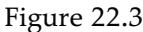
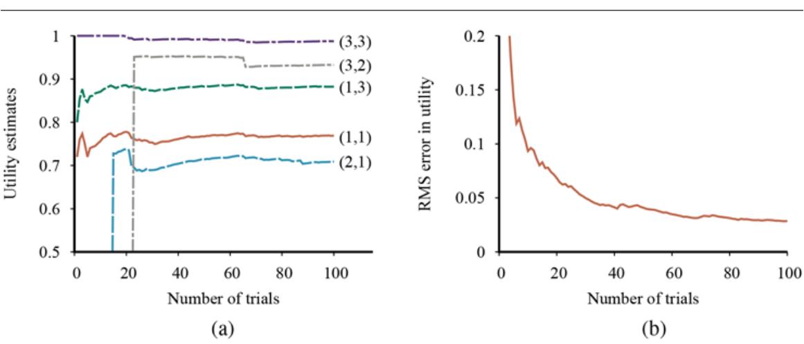
The passive ADP learning curves for the world, given the optimal policy shown in Figure 22.1 . (a) The utility estimates for a selected subset of states, as a function of the number of trials. Notice that it takes 14 and 23 trials respectively before the rarely visited states (2,1) and (3,2) “discover” that they connect to the exit state at (4,3). (b) The root-mean-square error (see Appendix A ) in the estimate for , averaged over 50 runs of 100 trials each.

22.2.3 Temporal-difference learning

Solving the underlying MDP as in the preceding section is not the only way to bring the Bellman equations to bear on the learning problem. Another way is to use the observed transitions to adjust the utilities of the observed states so that they agree with the constraint equations. Consider, for example, the transition from (1,3) to (2,3) in the second trial on page 792. Suppose that as a result of the first trial, the utility estimates are and . Now, if this transition from (1,3) to (2,3) occurred all the time, we would expect the utilities to obey the equation

\[U^{\pi}(1,3) = -0.04 + U^{\pi}(2,3),\]

so would be 0.92. Thus, its current estimate of 0.84 might be a little low and should be increased. More generally, when a transition occurs from state to state via action , we apply the following update to :

(22.3)

\[U^{\pi}(s) \leftarrow U^{\pi}(s) + \alpha[R(s, \pi(s), s') + \gamma U^{\pi}(s') - U^{\pi}(s)],\]

Here, is the learning rate parameter. Because this update rule uses the difference in utilities between successive states (and thus successive times), it is often called the temporal-difference (TD) equation. Just as in the weight update rules from Chapter 19 (e.g., Equation (19.6) on page 680), the TD term is effectively an error signal, and the update is intended to reduce the error.

Temporal-difference

All temporal-difference methods work by adjusting the utility estimates toward the ideal equilibrium that holds locally when the utility estimates are correct. In the case of passive learning, the equilibrium is given by Equation (22.2) . Now Equation (22.3) does in fact cause the agent to reach the equilibrium given by Equation (22.2) , but there is some subtlety involved. First, notice that the update involves only the observed successor , whereas the actual equilibrium conditions involve all possible next states. One might think that this causes an improperly large change in when a very rare transition occurs; but, in fact, because rare transitions occur only rarely, the average value of will converge to the correct quantity in the limit, even if the value itself continues to fluctuate.

Furthermore, if we turn the parameter into a function that decreases as the number of times a state has been visited increases, as shown in Figure 22.4 , then itself will converge to the correct value. Figure 22.5 illustrates the performance of the passive TD agent on the world. It does not learn quite as fast as the ADP agent and shows much higher variability, but it is much simpler and requires much less computation per observation. Notice that TD does not need a transition model to perform its updates. The environment itself supplies the connection between neighboring states in the form of observed transitions. 3

3 The technical conditions are given on page 684. In Figure 22.5 we have used , which satisfies the conditions.

Figure 22.4

A passive reinforcement learning agent that learns utility estimates using temporal differences. The stepsize function is chosen to ensure convergence.

Figure 22.5

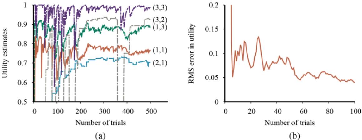
The TD learning curves for the world. (a) The utility estimates for a selected subset of states, as a function of the number of trials, for a single run of 500 trials. Compare with the run of 100 trials in Figure 22.3(a) . (b) The root-mean-square error in the estimate for , averaged over 50 runs of 100 trials each.

The ADP and TD approaches are closely related. Both try to make local adjustments to the utility estimates in order to make each state “agree” with its successors. One difference is that TD adjusts a state to agree with its observed successor (Equation (22.3) ), whereas ADP adjusts the state to agree with all of the successors that might occur, weighted by their probabilities (Equation (22.2) ). This difference disappears when the effects of TD adjustments are averaged over a large number of transitions, because the frequency of each successor in the set of transitions is approximately proportional to its probability. A more important difference is that whereas TD makes a single adjustment per observed transition, ADP makes as many as it needs to restore consistency between the utility estimates U and the transition model . Although the observed transition makes only a local change in , its effects might need to be propagated throughout U. Thus, TD can be viewed as a crude but efficient first approximation to ADP.

Each adjustment made by ADP could be seen, from the TD point of view, as a result of a pseudoexperience generated by simulating the current transition model. It is possible to extend the TD approach to use a transition model to generate several pseudoexperiences transitions that the TD agent can imagine might happen, given its current model. For each observed transition, the TD agent can generate a large number of imaginary transitions. In this way, the resulting utility estimates will approximate more and more closely those of ADP—of course, at the expense of increased computation time.

Pseudoexperience

In a similar vein, we can generate more efficient versions of ADP by directly approximating the algorithms for value iteration or policy iteration. Even though the value iteration algorithm is efficient, it is intractable if we have, say, states. However, many of the necessary adjustments to the state values on each iteration will be extremely tiny. One possible approach to generating reasonably good answers quickly is to bound the number of adjustments made after each observed transition. One can also use a heuristic to rank the possible adjustments so as to carry out only the most significant ones. The prioritized sweeping heuristic prefers to make adjustments to states whose likely successors have just undergone a large adjustment in their own utility estimates.

Prioritized sweeping

Using heuristics like this, approximate ADP algorithms can learn roughly as fast as full ADP, in terms of the number of training sequences, but can be orders of magnitude more efficient in terms of total computation (see Exercise 22.PRSW). This enables them to handle state spaces that are far too large for full ADP. Approximate ADP algorithms have an additional advantage: in the early stages of learning a new environment, the transition model often will be far from correct, so there is little point in calculating an exact utility function to match it. An approximation algorithm can use a minimum adjustment size that decreases as the transition model becomes more accurate. This eliminates the very long runs of value iteration that can occur early in learning due to large changes in the model.

22.3 Active Reinforcement Learning

A passive learning agent has a fixed policy that determines its behavior. An active learning agent gets to decide what actions to take. Let us begin with the adaptive dynamic programming (ADP) agent and consider how it can be modified to take advantage of this new freedom.

First, the agent will need to learn a complete transition model with outcome probabilities for all actions, rather than just the model for the fixed policy. The learning mechanism used by PASSIVE-ADP-AGENT will do just fine for this. Next, we need to take into account the fact that the agent has a choice of actions. The utilities it needs to learn are those defined by the optimal policy; they obey the Bellman equations (which we repeat here):

(22.4)

\[U(s) = \max\_{a \in A(s)} \sum\_{s'} P(s'|s, a) [R(s, a, s') + \gamma U(s')].\]

These equations can be solved to obtain the utility function using the value iteration or policy iteration algorithms from Chapter 17 .

The final issue is what to do at each step. Having obtained a utility function that is optimal for the learned model, the agent can extract an optimal action by one-step lookahead to maximize the expected utility; alternatively, if it uses policy iteration, the optimal policy is already available, so it could simply execute the action the optimal policy recommends. But should it?

22.3.1 Exploration

Figure 22.6 shows the results of one sequence of trials for an ADP agent that follows the recommendation of the optimal policy for the learned model at each step. The agent does not learn the true utilities or the true optimal policy! What happens instead is that in the third trial, it finds a policy that reaches the reward along the lower route via (2,1), (3,1), (3,2), and (3,3). (See Figure 22.6(b) .) After experimenting with minor variations, from the eighth trial onward it sticks to that policy, never learning the utilities of the other states and never

finding the optimal route via (1,2), (1,3), and (2,3). We will call this agent a greedy agent, because it greedily takes the action that it currently believes to be optimal at each step. Sometimes greed pays off and the agent converges to the optimal policy, but often it does not.

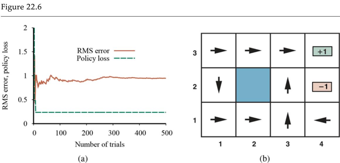
Performance of a greedy ADP agent that executes the action recommended by the optimal policy for the learned model. (a) The root mean square (RMS) error averaged across all nine nonterminal squares and the policy loss in (1,1). We see that the policy converges quickly, after just eight trials, to a suboptimal policy with a loss of 0.235. (b) The suboptimal policy to which the greedy agent converges in this particular sequence of trials. Notice the action in (1,2).

Greedy agent

How can it be that choosing the optimal action leads to suboptimal results? The answer is that the learned model is not the same as the true environment; what is optimal in the learned model can therefore be suboptimal in the true environment. Unfortunately, the agent does not know what the true environment is, so it cannot compute the optimal action for the true environment. What, then, should it do?

The greedy agent has overlooked the fact that actions do more than provide rewards; they also provide information in the form of percepts in the resulting states. As we saw with bandit problems in Section 17.3 , an agent must make a tradeoff between exploitation of the current best action to maximize its short-term reward and exploration of previously unknown states to gain information that can lead to a change in policy (and to greater rewards in the future). In the real world, one constantly has to decide between continuing in a comfortable existence, versus striking out into the unknown in the hopes of a better life.

Although bandit problems are difficult to solve exactly to obtain an optimal exploration scheme, it is nonetheless possible to come up with a scheme that will eventually discover an optimal policy, even if it might take longer to do so than is optimal. Any such scheme should not be greedy in terms of the immediate next move, but should be what is called “greedy in the limit of infinite exploration,” or GLIE. A GLIE scheme must try each action in each state an unbounded number of times to avoid having a finite probability that an optimal action is missed. An ADP agent using such a scheme will eventually learn the true transition model, and can then operate under exploitation.

GLIE

There are several GLIE schemes; one of the simplest is to have the agent choose a random action at time step with probability and to follow the greedy policy otherwise. While this does eventually converge to an optimal policy, it can be slow. A better approach would give some weight to actions that the agent has not tried very often, while tending to avoid actions that are believed to be of low utility (as we did with Monte Carlo tree search in Section 5.4 ). This can be implemented by altering the constraint equation (22.4) so that it assigns a higher utility estimate to relatively unexplored state–action pairs.

This amounts to an optimistic prior over the possible environments and causes the agent to behave initially as if there were wonderful rewards scattered all over the place. Let us use to denote the optimistic estimate of the utility (i.e., the expected reward-to-go) of the state , and let be the number of times action has been tried in state . Suppose we are using value iteration in an ADP learning agent; then we need to rewrite the update equation (Equation (17.10) on page 573) to incorporate the optimistic estimate:

\[U^{+}(s) \leftarrow \max\_{a} f\left(\sum\_{s'} P(s'|s,a)[R(s,a,s') + \gamma U^{+}(s')], N(s,a)\right).\]

Here, is the exploration function. The function determines how greed (preference for high values of the utility ) is traded off against curiosity (preference for actions that have not been tried often and have a low count ). The function should be increasing in and decreasing in . Obviously, there are many possible functions that fit these conditions. One particularly simple definition is

\[f(u,n) = \begin{cases} R^+ & \text{if } n < N\_e \\ u & \text{otherwise,} \end{cases}\]

Exploration function

where is an optimistic estimate of the best possible reward obtainable in any state and is a fixed parameter. This will have the effect of making the agent try each state–action pair at least times. The fact that rather than appears on the right-hand side of Equation (22.5) is very important. As exploration proceeds, the states and actions near the start state might well be tried a large number of times. If we used , the more pessimistic utility estimate, then the agent would soon become disinclined to explore further afield. The use of means that the benefits of exploration are propagated back from the edges of unexplored regions, so that actions that lead toward unexplored regions are weighted more highly, rather than just actions that are themselves unfamiliar.

The effect of this exploration policy can be seen clearly in Figure 22.7(b) , which shows a rapid convergence toward zero policy loss, unlike with the greedy approach. A very nearly optimal policy is found after just 18 trials. Notice that the RMS error in the utility estimates does not converge as quickly. This is because the agent stops exploring the unrewarding parts of the state space fairly soon, visiting them only “by accident” thereafter. However, it makes perfect sense for the agent not to care about the exact utilities of states that it knows are undesirable and can be avoided. There is not much point in learning about the best radio station to listen to while falling off a cliff.

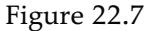
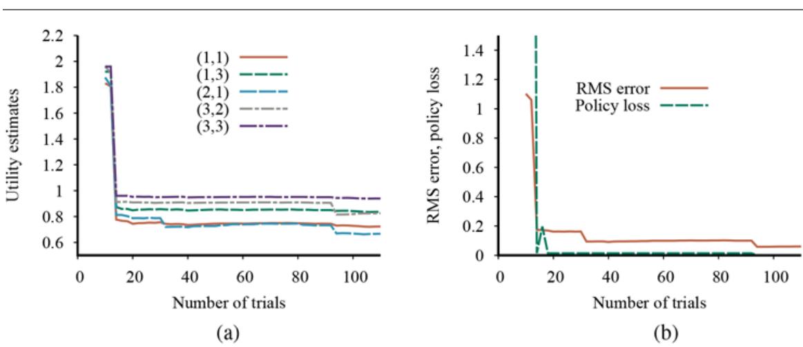
Performance of the exploratory ADP agent using and . (a) Utility estimates for selected states over time. (b) The RMS error in utility values and the associated policy loss.

22.3.2 Safe exploration

So far we have assumed that an agent is free to explore as it wishes—that any negative rewards serve only to improve its model of the world. That is, if we play a game of chess and lose, we suffer no damage (except perhaps to our pride), and whatever we learned will make us a better player in the next game. Similarly, in a simulation environment for a selfdriving car, we could explore the limits of the car’s performance, and any accidents give us more information. If the car crashes, we just hit the reset button.

Unfortunately, the real world is less forgiving. If you are a baby sunfish, your probability of surviving to adulthood is about 0.00000001. Many actions are irreversible, in the sense defined for online search agents in Section 4.5 : no subsequent sequence of actions can restore the state to what it was before the irreversible action was taken. In the worst case, the agent enters an absorbing state where no actions have any effect and no rewards are received.

Absorbing state

In many practical settings, we cannot afford to have our agents taking irreversible actions or entering absorbing states. For example, an agent learning to drive in a real car should avoid taking actions that might lead to any of the following:

• states with large negative rewards, such as serious car crashes;
• states from which there is no escape, such as driving the car into a deep ditch;
• states that permanently limit future rewards, such as damaging the car’s engine so that its maximum speed is reduced.

We can end up in a bad state either because our model is unknown, and we actively choose to explore in a direction that turns out to be bad, or because our model is incorrect and we don’t know that a given action can have a disastrous result. Note that the algorithm in Figure 22.2 is using maximum-likelihood estimation (see Chapter 20 ) to learn the transition model; moreover, by choosing a policy based solely on the estimated model, it is acting as if the model were correct. This is not necessarily a good idea! For example, a taxi agent that didn’t know how traffic lights work might ignore a red light once or twice with no ill effects and then formulate a policy to ignore all red lights from then on.

A better idea would be to choose a policy that works reasonably well for the whole range of models that have a reasonable chance of being the true model, even if the policy happens to be suboptimal for the maximum-likelihood model. There are three mathematical approaches that have this flavor.

The first approach, Bayesian reinforcement learning, assumes a prior probability over hypotheses about what the true model is; the posterior probability is obtained in the usual way by Bayes’ rule given the observations to date. Then, if the agent has decided to stop learning, the optimal policy is the one that gives the highest expected utility. Let be the expected utility, averaged over all possible start states, obtained by executing policy in model . Then we have

\[ \pi^\* = \underset{\pi}{\text{argmax}} \sum\_h P(h|\mathbf{e}) U\_h^{\pi}. \]

Bayesian reinforcement learning

In some special cases, this policy can even be computed! If the agent will continue learning in the future, however, then finding an optimal policy becomes considerably more difficult, because the agent must consider the effects of future observations on its beliefs about the transition model. The problem becomes an exploration POMDP whose belief states are distributions over models. In principle, this exploration POMDP can be formulated and solved before the agent ever sets foot in the world. (Exercise 22.EPOM asks you to do this for the Minesweeper game to find the best first move.) The result is a complete strategy that tells the agent what to do next given any possible percept sequence. Solving the exploration POMDP is usually wildly intractable, but the concept provides an analytical foundation for understanding the exploration problem described in Section 22.3 .

Exploration POMDP

It is worth noting that being perfectly Bayesian will not protect the agent from an untimely death. Unless the prior gives some indication of percepts that suggest danger, there is nothing to prevent the agent from taking an exploratory action that leads to an absorbing state. For example, it used to be thought that human infants had an innate fear of heights and would not crawl off a cliff, but this turns out not to be true (Adolph et al., 2014).

The second approach, derived from robust control theory, allows for a set of possible models without assigning probabilities to them, and defines an optimal robust policy as one that gives the best outcome in the worst case over :

\[ \pi^\* = \underset{\pi}{\text{argmax}} \,\underset{h}{\text{min}} U\_h^{\pi}. \]

Robust control theory

Often, the set will be the set of models that exceed some likelihood threshold on , so the robust and Bayesian approaches are related.

The robust control approach can be considered as a game between the agent and an adversary, where the adversary gets to pick the worst possible result for any action, and the policy we get is the minimax solution for the game. Our logical wumpus agent (see Section 7.7 ) is a robust control agent in this way: it considers all models that are logically possible, and does not explore any locations that could possibly contain a pit or a wumpus, so it is finding the action with maximum utility in the worst case over all possible hypotheses.

The problem with the worst-case assumption is that it results in overly conservative behavior. A self-driving car that assumes that every other driver will try to collide with it has no choice but to stay in the garage. Real life is full of such risk–reward tradeoffs.

Although one reason for venturing into reinforcement learning was to escape the need for a human teacher (as in supervised learning), it turns out that human knowledge can help keep a system safe. One way is to record a series of actions by an experienced teacher, so that the system will act reasonably from the start, and can learn to improve from there. A second way is for a human to write down constraints on what a system can do, and have a program outside of the reinforcement learning system enforce those constraints. For example, when training an autonomous helicopter, a partial policy can be provided that takes over control when the helicopter enters a state from which any further unsafe actions would lead to an irrecoverable state—one in which the safety controller cannot guarantee that the absorbing state will be avoided. In all other states, the learning agent is free to do as it pleases.

22.3.3 Temporal-difference Q-learning

Now that we have an active ADP agent, let us consider how to construct an active temporaldifference (TD) learning agent. The most obvious change is that the agent will have to learn a transition model so that it can choose an action based on via one-step look-ahead. The model acquisition problem for the TD agent is identical to that for the ADP agent, and the TD update rule remains unchanged. Once again, it can be shown that the TD algorithm will converge to the same values as ADP, as the number of training sequences tends to infinity.

The Q-learning method avoids the need for a model by learning an action-utility function instead of a utility function . denotes the expected total discounted reward if the agent takes action in and acts optimally thereafter. Knowing the Q-function enables the agent to act optimally simply by choosing , with no need for look-ahead based on a transition model.

We can also derive a model-free TD update for the Q-values. We begin with the Bellman equation for , repeated here from Equation (17.8) :

(22.6)

\[Q(s,a) = \sum\_{s'} P(s'|s,a)[R(s,a,s') + \gamma \max\_{a'} Q(s',a')]\]

From this, we can write down the Q-learning TD update, by analogy to the TD update for utilities in Equation (22.3) :

(22.7)

\[Q(s,a) \leftarrow Q(s,a) + \alpha[R(s,a,s') + \gamma \max\_{a'} Q(s',a') - Q(s,a)].\]

This update is calculated whenever action is executed in state leading to state . As in Equation (22.3) , the term represents an error that the update is trying to minimize.

The important part of this equation is what it does not contain: a TD Q-learning agent does not need a transition model, , either for learning or for action selection. As noted at the beginning of the chapter, model-free methods can be applied even in very complex domains because no model need be provided or learned. On the other hand, the Q-learning agent has no means of looking into the future, so it may have difficulty when rewards are sparse and long action sequences must be constructed to reach them.

The complete agent design for an exploratory TD Q-learning agent is shown in Figure 22.8 . Notice that it uses exactly the same exploration function as that used by the exploratory ADP agent—hence the need to keep statistics on actions taken (the table ). If a simpler exploration policy is used—say, acting randomly on some fraction of steps, where the fraction decreases over time—then we can dispense with the statistics.

An exploratory Q-learning agent. It is an active learner that learns the value of each action in each situation. It uses the same exploration function as the exploratory ADP agent, but avoids having to learn the transition model.

Q-learning has a close relative called SARSA (for state, action, reward, state, action). The update rule for SARSA is very similar to the Q-learning update rule (Equation (22.7) ), except that SARSA updates with the Q-value of the action that is actually taken:

(22.8)

\[Q(s,a) \leftarrow Q(s,a) + \alpha[R(s,a,s') + \gamma \, Q(s',a') - Q(s,a)],\]

SARSA

The rule is applied at the end of each quintuplet—hence the name. The difference from Q-learning is quite subtle: whereas Q-learning backs up the Q-value from the best action in , SARSA waits until an action is taken and backs up the Q-value for that action. If the agent is greedy and always takes the action with the best Q-value, the two algorithms are identical. When exploration is happening, however, they differ: if the exploration yields a negative reward, SARSA penalizes the action, while Q-learning does not.

Q-learning is an off-policy learning algorithm, because it learns Q-values that answer the question “What would this action be worth in this state, assuming that I stop using whatever policy I am using now, and start acting according to a policy that chooses the best action

(according to my estimates)?” SARSA is an on-policy algorithm: it learns Q-values that answer the question “What would this action be worth in this state, assuming I stick with my policy?” Q-learning is more flexible than SARSA, in the sense that a Q-learning agent can learn how to behave well when under the control of a wide variety of exploration policies. On the other hand, SARSA is appropriate if the overall policy is even partly controlled by other agents or programs, in which case it is better to learn a Q-function for what will actually happen rather than what would happen if the agent got to pick estimated best actions. Both Q-learning and SARSA learn the optimal policy for the world, but they do so at a much slower rate than the ADP agent. This is because the local updates do not enforce consistency among all the Q-values via the model.

Off-policy

On-policy

22.4 Generalization in Reinforcement Learning

So far, we have assumed that utility functions and Q-functions are represented in tabular form with one output value for each state. This works for state spaces with up to about states, which is more than enough for our toy two-dimensional grid environments. But in real-world environments with many more states, convergence will be too slow. Backgammon is simpler than most real-world applications, yet it has about states. We cannot easily visit them all in order to learn how to play the game.

Chapter 5 introduced the idea of an evaluation function as a compact measure of desirability for potentially vast state spaces. In the terminology of this chapter, the evaluation function is an approximate utility function; we use the term function approximation for the process of constructing a compact approximation of the true utility function or Q-function. For example, we might approximate the utility function using a weighted linear combination of features :

\[ \hat{U}\_\theta(s) = \theta\_1 f\_1(s) + \theta\_2 f\_2(s) + \dots + \theta\_n f\_n(s). \]

Function approximation

Instead of learning state values in a table, a reinforcement learning algorithm can learn, say, 20 values for the parameters that make a good approximation to the true utility function. Sometimes this approximate utility function is combined with lookahead search to produce more accurate decisions. Adding look-ahead search means that effective behavior can be generated from a much simpler utility function approximator that is learnable from far fewer experiences.

Function approximation makes it practical to represent utility (or Q) functions for very large state spaces, but more importantly, it allows for inductive generalization: the agent can generalize from states it has visited to states it has not yet visited. Tesauro (1992) used this

technique to build a backgammon-playing program that played at human champion level, even though it explored only a trillionth of the complete state space of backgammon.

22.4.1 Approximating direct utility estimation

The method of direct utility estimation (Section 22.2 ) generates trajectories in the state space and extracts, for each state, the sum of rewards received from that state onward until termination. The state and the sum of rewards received constitute a training example for a supervised learning algorithm. For example, suppose we represent the utilities for the world using a simple linear function, where the features of the squares are just their and coordinates. In that case, we have

(22.9)

\[ \ddot{U}\_\theta(x, y) = \theta\_0 + \theta\_1 x + \theta\_2 y. \]

Thus, if , then . Given a collection of trials, we obtain a set of sample values of , and we can find the best fit, in the sense of minimizing the squared error, using standard linear regression (see Chapter 19 ).

For reinforcement learning, it makes more sense to use an online learning algorithm that updates the parameters after each trial. Suppose we run a trial and the total reward obtained starting at (1,1) is 0.4. This suggests that , currently 0.8, is too large and must be reduced. How should the parameters be adjusted to achieve this? As with neural-network learning, we write an error function and compute its gradient with respect to the parameters. If is the observed total reward from state onward in the th trial, then the error is defined as (half) the squared difference of the predicted total and the actual total: . The rate of change of the error with respect to each parameter is , so to move the parameter in the direction of decreasing the error, we want

(22.10)

\[ \theta\_i \leftarrow \theta\_i - \alpha \frac{\partial E\_j(s)}{\partial \theta\_i} = \theta\_i + \alpha [u\_j(s) - \hat{U}\_\theta(s)] \frac{\partial \hat{U}\_\theta(s)}{\partial \theta\_i} \]

This is called the Widrow–Hoff rule, or the delta rule, for online least-squares. For the linear function approximator in Equation (22.9) , we get three simple update rules:

\[\theta\_0 \gets \theta\_0 + \alpha[u\_j(s) - \hat{U}\_\theta(s)],\]

\[\theta\_1 \gets \theta\_1 + \alpha[u\_j(s) - \hat{U}\_\theta(s)]x,\]

\[\theta\_2 \gets \theta\_2 + \alpha[u\_j(s) - \hat{U}\_\theta(s)]y.\]

Widrow–Hoff rule

Delta rule

We can apply these rules to the example where is 0.8 and is 0.4. Parameters , , and are all decreased by , which reduces the error for (1,1). Notice that changing the parameters in response to an observed transition between two states also changes the values of for every other state! This is what we mean by saying that function approximation allows a reinforcement learner to generalize from its experiences.

The agent will learn faster if it uses a function approximator, provided that the hypothesis space is not too large and includes some functions that are a reasonably good fit to the true utility function. Exercise 22.APLM asks you to evaluate the performance of direct utility estimation, both with and without function approximation. The improvement in the world is noticeable but not dramatic, because this is a very small state space to begin with. The improvement is much greater in a world with a reward at (10,10).

The world is well suited for a linear utility function because the true utility function is smooth and nearly linear: it is basically a diagonal slope with its lower corner at (1,1) and its upper corner at (10,10). (See Exercise 22.TENX.) On the other hand, if we put the reward at (5,5), the true utility is more like a pyramid and the function approximator in Equation (22.9) will fail miserably.

All is not lost, however! Remember that what matters for linear function approximation is that the function be linear in the features. But we can choose the features to be arbitrary nonlinear functions of the state variables. Hence, we can include a feature such as

that measures the distance to the goal. With this new feature, the linear function approximator does well.

22.4.2 Approximating temporal-difference learning

We can apply these ideas equally well to temporal-difference learners. All we need do is adjust the parameters to try to reduce the temporal difference between successive states. The new versions of the TD and Q-learning equations (22.3 on page 795 and 22.7 on page 802) are given by

(22.11)

\[\theta\_i \gets \theta\_i + \alpha[R(s, a, s') + \gamma \hat{U}\_\theta(s') - \hat{U}\_\theta(s)]\frac{\partial U\_\theta(s)}{\partial \theta\_i}\]

for utilities and

(22.12)

\[\theta\_i \gets \theta\_i + \alpha[R(s, a, s') + \gamma \max\_{a'} \hat{Q}\_{\theta}(s', a') - \hat{Q}\_{\theta}(s, a)] \frac{\partial \ddot{Q}\_{\theta}(s, a)}{\partial \theta\_i}.\]

for Q-values. For passive TD learning, the update rule can be shown to converge to the closest possible approximation to the true function when the function approximator is linear in the features. With active learning and nonlinear functions such as neural networks, nearly all bets are off: there are some very simple cases in which the parameters can go off to infinity with these update rules, even though there are good solutions in the hypothesis space. There are more sophisticated algorithms that can avoid these problems, but at present reinforcement learning with general function approximators remains a delicate art. 4

4 The definition of distance between utility functions is rather technical; see Tsitsiklis and Van Roy (1997).

In addition to parameters diverging to infinity, there is a more surprising problem called catastrophic forgetting. Suppose you are training an autonomous vehicle to drive along (simulated) roads safely without crashing. You assign a high negative reward for crossing the edge of the road, and you use quadratic features of the road position so that the car can learn that the utility of being in the middle of the road is higher than being close to the edge. All goes well, and the car learns to drive perfectly down the middle of the road. After a few minutes of this, you are starting to get bored and are about to halt the simulation and write up the excellent results. All of a sudden, the vehicle swerves off the road and crashes. Why? What has happened is that the car has learned too well: because it has learned to steer away from the edge, it has learned that the entire central region of the road is a safe place to be, and it has forgotten that the region closer to the edge is dangerous. The central region therefore has a flat value function, so the quadratic features get zero weight; then, any nonzero weight on the linear features causes the car to slide off the road to one side or the other.

Catastrophic forgetting

One solution to this problem, called experience replay, ensures that the car keeps reliving its youthful crashing behavior at regular intervals. The learning algorithm can retain trajectories from the entire learning process and replay those trajectories to ensure that its value function is still accurate for parts of the state space it no longer visits.

Experience replay

For model-based reinforcement learning systems, function approximation can also be very helpful for learning a model of the environment. Remember that learning a model for an observable environment is a supervised learning problem, because the next percept gives the outcome state. Any of the supervised learning methods in Chapters 19 –21 can be used, with suitable adjustments for the fact that we need to predict a complete state description rather than just a Boolean classification or a single real value. With a learned model, the agent can do a look-ahead search to improve its decisions and can carry out internal simulations to improve its approximate representations of or rather than requiring slow and potentially expensive real-world experiences.

For a partially observable environment, the learning problem is much more difficult because the next percept is no longer a label for the state prediction problem. If we know what the hidden variables are and how they are causally related to each other and to the observable variables, then we can fix the structure of a dynamic Bayesian network and use the EM algorithm to learn the parameters, as was described in Chapter 20 . Learning the internal structure of dynamic Bayesian networks and creating new state variables is still considered a difficult problem. Deep recurrent neural networks (Section 21.6 ) have in some cases been successful at inventing the hidden structure.

22.4.3 Deep reinforcement learning

There are two reasons why we need to go beyond linear function approximators: first, there may be no good linear function that comes close to approximating the utility function or the Q-function; second, we may not be able to invent the necessary features, particularly in new domains. If you think about it, these are really the same reason: it is always possible to represent or as linear combinations of features, especially if we have features such as or , but unless we can come up with such features (in an efficiently computable form) the linear function approximator may be insufficient.

For these reasons (or reason), researchers have explored more complex, nonlinear function approximators since the earliest days of reinforcement learning. Currently, deep neural networks (Chapter 21 ) are very popular in this role and have proved to be effective even when the input is a raw image with no human-designed feature extraction at all. If all goes well, the deep neural network in effect discovers the useful features for itself. And if the final layer of the network is linear, then we can see what features the network is using to build its own linear function approximator. A reinforcement learning system that uses a deep network as a function approximator is called a deep reinforcement learning system.

Just as in Equation (22.9) , the deep network is a function parameterized by , except that now the function is much more complicated. The parameters are all the weights in all the layers of the network. Nonetheless, the gradients required for Equations (22.11) and (22.12) are just the same as the gradients required for supervised learning, and they can be computed by the same back-propagation process described in Section 21.4 .

As we explain in Section 22.7 , deep RL has achieved very significant results, including learning to play a wide range of video games at an expert level, defeating the human world champion at Go, and training robots to perform complex tasks.

Despite its impressive successes, deep RL still faces significant obstacles: it is often difficult to get good performance and the trained system may behave very unpredictably if the environment differs even a little from the training data. Compared to other applications of deep learning, deep RL is rarely applied in commercial settings. It is, nonetheless, a very active area of research.

22.4.4 Reward shaping

As noted in the introduction to this chapter, real-world environments may have very sparse rewards: many primitive actions are required to achieve any nonzero reward. For example, a soccer-playing robot might send a hundred thousand motor control commands to its various joints before conceding a goal. Now it has to work out what it did wrong. The technical term for this is the credit assignment problem. Other than playing trillions of soccer games so that the negative reward eventually propagates back to the actions responsible for it, is there a good solution?

Credit assignment

One common method, originally used in animal training, is called reward shaping. This involves supplying the agent with additional rewards, called pseudorewards, for “making progress.” For example, we might give pseudorewards to the robot for making contact with the ball or for advancing it toward the goal. Such rewards can speed up learning enormously and are simple to provide, but there is a risk that the agent will learn to maximize the pseudorewards rather than the true rewards; for example, standing next to the ball and “vibrating” causes many contacts with the ball.

Reward shaping

Pseudoreward

In Chapter 17 (page 569), we saw a way to modify the reward function without changing the optimal policy. For any potential function and any reward function , we can create a new reward function as follows:

\[R'(s, a, s') = R(s, a, s') + \gamma \Phi(s') - \Phi(s).\]

The potential fuction can be constructed to reflect any desirable aspects of the state, such as achievement of subgoals or distance to a desired terminal state. For example, for the soccer-playing robot could add a constant bonus for states where the robot’s team has possession and another bonus for reducing the distance of the ball from the opponents’ goal. This will result in faster learning overall, but will not prevent the robot from, say, learning to pass back to the goalkeeper when danger threatens.

22.4.5 Hierarchical reinforcement learning

Hierarchical reinforcement learning

Another way to cope with very long action sequences is to break them up into a few smaller pieces, and then break those into smaller pieces still, and so on until the action sequences are short enough to make learning easy. This approach is called hierarchical reinforcement learning (HRL), and it has much in common with the HTN planning methods described in Chapter 11 . For example, scoring a goal in soccer can be broken down into obtaining possession, passing to a teammate, receiving the ball from a team-mate, dribbling toward the goal, and shooting; each of these can be broken down further into lower-level motor behaviors. Obviously, there are multiple ways of obtaining possession and shooting, multiple teammates one could pass to, and so on, so each higher-level action may have many different lower-level implementations.

To illustrate these ideas, we’ll use a simplified soccer game called keepaway, in which one team of three players tries to keep possession of the ball for as long as possible by dribbling and passing amongst themselves while the other team of two players tries to take possession by intercepting a pass or tackling a player in possession. The game is implemented within the RoboCup 2D simulator, which provides detailed continuous-state motion models with 100ms time steps and has proved to be a good testbed for RL systems. 5

5 Rumors that keepaway was inspired by the real-world tactics of Barcelona FC are probably unfounded.

Keepaway

A hierarchical reinforcement learning agent begins with a partial program that outlines a hierarchical structure for the agent’s behavior. The partial-programming language for agent programs extends any ordinary programming language by adding primitives for unspecified choices that must be filled in by learning. (Here, we use pseudocode for the programming language.) The partial program can be arbitrarily complicated, as long as it terminates.

Partial program

It is easy to see that HRL includes ordinary RL as a special case. We simply provide the trivial partial program that allows the agent to keep choosing any action from , the set of actions that can be executed in the current state :

while true do choose(A(s)). The choose operator allows the agent to choose any element of the specified set. The learning process converts the partial agent program into a complete program by learning how each choice should be made. For example, the learning process might associate a Qfunction with each choice; once the Q-functions are learned, the program produces behavior by choosing the option with the highest Q-value each time it encounters a choice.

The agent programs for keepaway are more interesting. We’ll look at the partial program for a single player on the “keeper” team. The choice of what to do at the top level depends mainly on whether the player has the ball or not:

while not IS-TERMINAL(s) do
 if BALL-IN-MY-POSSESSION(s) then choose({PASS,HOLD,DRIBBLE})
 else choose({STAY,MOVE, INTERCEPT-BALL}).

Each of these choices invokes a subroutine that may itself make further choices, all the way down to primitive actions that can be executed directly. For example, the high-level action PASS chooses a teammate to pass to, but also has the choice to do nothing and return control to the higher level if appropriate (e.g., if there is no one to pass to):

choose({PASS-TO(choose(TEAMMATES(s))), return}).

The PASS-TO routine then has to choose a speed and direction for the pass. While it is relatively easy for a human—even one with little expertise in soccer—to provide this kind of high-level advice to the learning agent, it would be difficult, if not impossible, to write down the rules for determining the speed and direction of the kick to maximize the probability of maintaining possession. Similarly, it is far from obvious how to choose the right teammate to receive the ball or where to move in order to make oneself available to receive the ball. The partial program provides general know-how—overall scaffolding and structural organization for complex behaviors—and the learning process works out all the details.

The theoretical foundations of HRL are based on the concept of the joint state space, in which each state is composed of a physical state and a machine state . The machine state is defined by the current internal state of the agent program: the program counter for each subroutine on the current call stack, the values of the arguments, and the values of all local and global variables. For example, if the agent program has chosen to pass to teammate Ali and is in the middle of calculating the speed of the pass, then the fact that Ali is the argument of PASS-TO is part of the current machine state. A choice state is one in which the program counter for is at a choice point in the agent program. Between two choice states, any number of computational transitions and physical actions may occur, but they are all preordained, so to speak: by definition, the agent isn’t making any choices in between choice states. Essentially, the hierarchical RL agent is solving a Markovian decision problem with the following elements:

• The states are the choice states of the joint state space.
• The actions at are the choices available in according to the partial program.
• The reward function is the expected sum of rewards for all physical transitions occurring between the choice states and .
• The transition model is defined in the obvious way: if invokes a physical action , then borrows from the physical model ; if invokes a computational transition, such as calling a subroutine, then the transition deterministically modifies the computational state according to the rules of the programming language. 6

6 Because more than one physical action may be executed before the next choice state is reached, the problem is technically a semi-Markov decision process, which allows actions to have different durations, including stochastic durations. If the discount factor , then the action duration affects the discounting applied to the reward obtained during the action, which means that some extra discount bookkeeping has to be done and the transition model includes the duration distribution.

Joint state space

Choice state

By solving this decision problem, the agent finds the optimal policy that is consistent with original partial program.

Hierarchical RL can be a very effective method for learning complex behaviors. In keepaway, an HRL agent based on the partial program sketched above learns a policy that keeps possession forever against the standard taker policy—a significant improvement on the previous record of about 10 seconds. One important characteristic is that the lower-level skills are not fixed subroutines in the usual sense; their choices are sensitive to the entire internal state of the agent program, so they behave differently depending on where they are invoked within that program and what is going on at the time. If necessary, the Q-functions for the lower-level choices can be initialized by a separate training process with its own reward function, and then integrated into the overall system so they can be adapted to function well in the context of the whole agent.

In the preceding section we saw that shaping rewards can be helpful for learning complex behaviors. In HRL, the fact that learning takes place in the joint state space provides additional opportunities for shaping. For example, to help with learning the Q-function for accurate passing within the PASS-TO routine, we can provide a shaping reward that depends on the location of the intended recipient and the proximity of opponents to that player: the ball should be close to the recipient and far from the opponents. That seems entirely obvious; but the identity of the intended recipient for a pass is not part of the physical state of the world. The physical state consists only of the positions, orientations, and velocities of the players and the ball. There is no “passing” and no “recipient” in the physical world; these are entirely internal constructs. This means that there is no way to provide such sensible advice to a standard RL system.

The hierarchical structure of behavior also provides a natural additive decomposition of the overall utility function. Remember that utility is the sum of rewards over time, and consider a sequence of, say, ten time steps with rewards . Suppose that for the first five time steps the agent is doing PASS-TO(Ali) and for the remaining five steps it is doing MOVE-INTO-SPACE. Then the utility for the initial state is the sum of the total reward during PASS-TO and the total reward during MOVE-INTO-SPACE. The former depends only on whether the ball gets to Ali with enough time and space for Ali to retain possession, and the latter depends only on whether the agent reaches a good location to receive the ball. In other words, the overall utility decomposes into several terms, each of which depends on only a few

variables. This, in turns, means that learning occurs much more quickly than if we try to learn a single utility function that depends on all the variables. This is somewhat analogous to the representation theorems underlying the conciseness of Bayes nets (Chapter 13 ).

Additive decomposition

22.5 Policy Search

The final approach we will consider for reinforcement learning problems is called policy search. In some ways, policy search is the simplest of all the methods in this chapter: the idea is to keep twiddling the policy as long as its performance improves, then stop.

Policy search

Let us begin with the policies themselves. Remember that a policy is a function that maps states to actions. We are interested primarily in parameterized representations of that have far fewer parameters than there are states in the state space (just as in the preceding section). For example, we could represent by a collection of parameterized Q-functions, one for each action, and take the action with the highest predicted value:

(22.13)

\[ \pi(s) = \operatorname\*{argmax}\_{a} \hat{Q}\_{\theta}(s, a). \]

Each Q-function could be a linear function, as in Equation (22.9) , or it could be a nonlinear function such as a deep neural network. Policy search will then adjust the parameters to improve the policy. Notice that if the policy is represented by Q-functions, then policy search results in a process that learns Q-functions. This process is not the same as Q-learning!

In Q-learning with function approximation, the algorithm finds a value of such that is “close” to , the optimal Q-function. Policy search, on the other hand, finds a value of that results in good performance; the values found by the two methods may differ very substantially. (For example, the approximate Q-function defined by gives optimal performance, even though it is not at all close to .) Another clear instance of the difference is the case where is calculated using, say, depth-10 look-ahead search with an approximate utility function . A value of that gives good results may be a long way from making resemble the true utility function.

One problem with policy representations of the kind given in Equation (22.13) is that the policy is a discontinuous function of the parameters when the actions are discrete. That is, there will be values of such that an infinitesimal change in causes the policy to switch from one action to another. This means that the value of the policy may also change discontinuously, which makes gradient-based search difficult. For this reason, policy search methods often use a stochastic policy representation , which specifies the probability of selecting action in state . One popular representation is the softmax function:

(22.14)

\[ \pi\_\theta(s, a) = \frac{e^{\beta Q\_\theta(s, a)}}{\sum\_{a'} e^{\beta \hat{Q}\_\theta(s, a')}}. \]

Stochastic policy

The parameter modulates the softness of the softmax: for values of that are large compared to the separations between Q-values, the softmax approaches a hard max, whereas for values of close to zero the softmax approaches a uniform random choice among the actions. For all finite values of , the softmax provides a differentiable function of ; hence, the value of the policy (which depends continuously on the action-selection probabilities) is a differentiable function of .

Now let us look at methods for improving the policy. We start with the simplest case: a deterministic policy and a deterministic environment. Let be the policy value, that is, the expected reward-to-go when is executed. If we can derive an expression for in closed form, then we have a standard optimization problem, as described in Chapter 4 . We can follow the policy gradient vector , provided is differentiable. Alternatively, if is not available in closed form, we can evaluate simply by executing it and observing the accumulated reward. We can follow the empirical gradient by hill climbing—that is, evaluating the change in policy value for small increments in each

parameter. With the usual caveats, this process will converge to a local optimum in policy space.

Policy value

Policy gradient

When the environment (or the policy) is nondeterministic, things get more difficult. Suppose we are trying to do hill climbing, which requires comparing and for some small . The problem is that the total reward for each trial may vary widely, so estimates of the policy value from a small number of trials will be quite unreliable; trying to compare two such estimates will be even more unreliable. One solution is simply to run lots of trials, measuring the sample variance and using it to determine that enough trials have been run to get a reliable indication of the direction of improvement for . Unfortunately, this is impractical for many real problems in which trials may be expensive, timeconsuming, and perhaps even dangerous.

For the case of a nondeterministic policy , it is possible to obtain an unbiased estimate of the gradient at , , directly from the results of trials executed at . For simplicity, we will derive this estimate for the simple case of an episodic environment in which each action obtains reward and the environment restarts in . In this case, the policy value is just the expected value of the reward, and we have

\[ \nabla\_{\theta} \rho(\theta) = \nabla\_{\theta} \sum\_{a} R(s\_0, a, s\_0) \pi\_{\theta}(s\_0, a) = \sum\_{a} R(s\_0, a, s\_0) \nabla\_{\theta} \pi\_{\theta}(s\_0, a). \]

Now we perform a simple trick so that this summation can be approximated by samples generated from the probability distribution defined by . Suppose that we have trials in all, and the action taken on the th trial is . Then

\[\begin{split} \nabla\_{\theta} \rho(\theta) &= \sum\_{a} \pi\_{\theta}(s\_{0}, a) \cdot \frac{R(s\_{0}, a, s\_{0}) \nabla\_{\theta} \pi\_{\theta}(s\_{0}, a)}{\pi\_{\theta}(s\_{0}, a)} \\ &= \approx \frac{1}{N} \sum\_{j=1}^{N} \frac{R(s\_{0}, a\_{j}, s\_{0}) \nabla\_{\theta} \pi\_{\theta}(s\_{0}, a\_{j})}{\pi\_{\theta}(s\_{0}, a\_{j})}. \end{split}\]

Thus, the true gradient of the policy value is approximated by a sum of terms involving the gradient of the action-selection probability in each trial. For the sequential case, this generalizes to

\[\nabla\_{\boldsymbol{\theta}}\rho(\boldsymbol{\theta}) \approx \frac{1}{N} \sum\_{j=1}^{N} \frac{u\_j(s)\nabla\_{\boldsymbol{\theta}}\pi\_{\boldsymbol{\theta}}(s,a\_j)}{\pi\_{\boldsymbol{\theta}}(s,a\_j)}\]

for each state visited, where is executed in on the th trial and is the total reward received from state onward in the th trial. The resulting algorithm, called REINFORCE, is due to Ron Williams (1992); it is usually much more effective than hill climbing using lots of trials at each value of . However, it is still much slower than necessary.

Consider the following task: given two blackjack policies, determine which is best. The policies might have true net returns per hand of, say, % and %, so finding out which is better is very important. One way to do this is to have each policy play against a standard “dealer” for a certain number of hands and then to measure their respective winnings. The problem with this, as we have seen, is that the winnings of each policy fluctuate wildly depending on whether it receives good or bad cards. One would need several million hands to have a reliable indication of which policy is better. The same issue arises when using random sampling to compare two adjacent policies in a hill-climbing algorithm.

A better solution for blackjack is to generate a certain number of hands in advance and have each program play the same set of hands. In this way, we eliminate the measurement error due to differences in the cards received. Only a few thousand hands are needed to determine which of the two blackjack policies is better.

This idea, called correlated sampling, can be applied to policy search in general, given an environment simulator in which the random-number sequences can be repeated. It was implemented in a policy-search algorithm called PEGASUS (Ng and Jordan, 2000), which was one of the first algorithms to achieve completely stable autonomous helicopter flight (see

Figure 22.9(b) ). It can be shown that the number of random sequences required to ensure that the value of every policy is well estimated depends only on the complexity of the policy space, and not at all on the complexity of the underlying domain.

1. Setup for the problem of balancing a long pole on top of a moving cart. The cart can be jerked left or right by a controller that observes the cart’s position and velocity , as well as the pole’s angle and rate of change of angle . (b) Six superimposed time-lapse images of a single autonomous helicopter performing a very difficult “nose-in circle” maneuver. The helicopter is under the control of a policy developed by the PEGASUS policy-search algorithm (Ng et al., 2003). A simulator model was developed by observing the effects of various control manipulations on the real helicopter; then the algorithm was run on the simulator model overnight. A variety of controllers were developed for different maneuvers. In all cases, performance far exceeded that of an expert human pilot using remote control. (Image courtesy of Andrew Ng.)

Correlated sampling

22.6 Apprenticeship and Inverse Reinforcement Learning

Some domains are so complex that it is difficult to define a reward function for use in reinforcement learning. Exactly what do we want our self-driving car to do? Certainly it should not take too long to get to the destination, but it should not drive so fast as to incur undue risk or to get speeding tickets. It should conserve fuel/energy. It should avoid jostling or accelerating the passengers too much, but it can slam on the brakes in an emergency. And so on. Deciding how much weight to give to each of these factors is a difficult task. Worse still, there are almost certainly important factors we have forgotten, such as the obligation to behave with consideration for other drivers. Omitting a factor usually leads to behavior that assigns an extreme value to the omitted factor—in this case, extremely inconsiderate driving—in order to maximize the remaining factors.

One approach is to do extensive testing in simulation, notice problematic behaviors, and try to modify the reward function to eliminate those behaviors. Another approach is to seek additional sources of information about the appropriate reward function. One such source is the behavior of agents who are already optimizing (or, let’s say, nearly optimizing) that reward function—in this case, expert human drivers.

The general field of apprenticeship learning studies the process of learning how to behave well given observations of expert behavior. We show the algorithm examples of expert driving and tell it to “do it like that.” There are (at least) two ways to approach the apprenticeship learning problem. The first is the one we discussed briefly at the beginning of the chapter: assuming the environment is observable, we apply supervised learning to the observed state–action pairs to learn a policy . This is called imitation learning. It has had some success in robotics (see page 966) but suffers from the the problem of brittleness: even small deviations from the training set lead to errors that grow over time and eventually to failure. Moreover, imitation learning will at best duplicate the teacher’s performance, not exceed it. When humans learn by imitation, we sometimes use the pejorative term “aping” to describe what they are doing. (It’s quite possible that apes use the term “humaning” amongst themselves, perhaps in an even more pejorative sense.) The implication is that the imitation learner doesn’t understand why it should perform any given action.

Apprenticeship learning

Imitation learning

The second approach to apprenticeship learning is to understand why: to observe the expert’s actions (and resulting states) and try to work out what reward function the expert is maximizing. Then we could derive an optimal policy with respect to that reward function. One expects that this approach will produce robust policies from relatively few examples of expert behavior; after all, the field of reinforcement learning is predicated on the idea that the reward function, rather than the policy or the value function, is the most succinct, robust, and transferable definition of the task. Furthermore, if the learner makes appropriate allowances for possible suboptimality on the part of the expert, then it may be able to do better than the expert by optimizing an accurate approximation to the true reward function. We call this approach inverse reinforcement learning (IRL): learning rewards by observing a policy, rather than learning a policy by observing rewards.

Inverse reinforcement learning

How do we find the expert’s reward function, given the expert’s actions? Let us begin by assuming that the expert was acting rationally. In that case, it seems we should be looking for a reward function such that the total expected discounted reward under the expert’s policy is higher than (or at least the same as) under any other possible policy.

Unfortunately, there will be many reward functions that satisfy this constraint; one of them is , because any policy is rational when there are no rewards at all. Another problem with this approach is that the assumption of a rational expert is unrealistic. It means, for example, that a robot observing Lee Sedol making what eventually turns out to 7

be a losing move against ALPHAGO would have to assume that Lee Sedol was trying to lose the game.

7 According to Equation (17.9) on page 569, a reward function has exactly the same optimal policies as , so we can recover the reward function only up to the possible addition of any shaping function . This is not such a serious problem, because a robot using will behave just like a robot using the “correct” .

To avoid the problem that explains any observed behavior, it helps to think in a Bayesian way. (See Section 20.1 for a reminder of what this means.) Suppose we observe data and let be the hypothesis that is the true reward function. Then according to Bayes’ rule, we have

\[P(h\_R|\mathbf{d}) = \alpha P(\mathbf{d}|h\_R)P(h\_R).\]

Now, if the prior is based on simplicity, then the hypothesis that scores fairly well, because 0 is certainly simple. On the other hand, the term is infinitesimal for the hypothesis that , because it doesn’t explain why the expert chose that particular behavior out of the vast space of behaviors that would be optimal if the hypothesis were true. On the other hand, for a reward function that has a unique optimal policy or a relatively small equivalence class of optimal policies, will be far higher.

To allow for the occasional mistake by the expert, we simply allow to be nonzero even when comes from behavior that is a little bit suboptimal according to . A typical assumption—made, it must be said, more for mathematical convenience than faithfulness to actual human data—is that an agent whose true Q-function is chooses not according to the deterministic policy but instead according to a stochastic policy defined by the softmax distribution from Equation (22.14) . This is sometimes called Boltzmann rationality because, in statistical mechanics, the state occupation probabilities in a Boltzmann distribution depend exponentially on their energy levels.

Boltzmann rationality

There are dozens of inverse RL algorithms in the literature. One of the simplest is called feature matching. It assumes that the reward function can be written as a weighted linear combination of features:

\[R\_{\theta}(s, a, s') = \sum\_{i=1}^{n} \theta\_i f\_i(s, a, s') = \theta \cdot \mathbf{f}.\]

Feature matching

For example, the features in the driving domain might include speed, speed in excess of the speed limit, acceleration, proximity to nearest obstacle, etc.

Recall from Equation (17.2) on page 567 that the utility of executing a policy , starting in state , is defined to be

\[U^{\pi}(s) = E\left[\sum\_{t=0}^{\infty} \gamma^t R(S\_t, \pi(S\_t), S\_{t+1})\right],\]

where the expectation is with respect to the probability distribution over state sequences determined by and . Because is assumed to be a linear combination of feature values, we can rewrite this as follows:

\[\begin{aligned} U^\pi(s) &= \left. E \left[ \sum\_{t=0}^\infty \gamma^t \sum\_{i=1}^n \theta\_i f\_i(S\_t, \pi(S\_t), S\_{t+1}) \right] \right| \\ &= \left. \sum\_{i=1}^n \theta\_i E \left[ \sum\_{t=0}^\infty \gamma^t f\_i(S\_t, \pi(S\_t), S\_{t+1}) \right] \right| \\ &= \left. \sum\_{i=1}^n \theta\_i \mu\_i(\pi) = \theta \cdot \mu(\pi) \right. \end{aligned}\]

Feature expectation

where we have defined the feature expectation as the expected discounted value of the feature when policy is executed. For example, if is the excess speed of the vehicle (above the speed limit), then is the (time-discounted) average excess speed over the entire trajectory. The key point about feature expectations is the following: if a policy produces feature expectations that match those of the expert’s policy , then is as good as the expert’s policy according to the expert’s own reward function. Now, we cannot measure the exact values for the feature expectations of the expert’s policy, but we can approximate them using the average values on the observed trajectories. Thus, we need to find values for the parameters such that the feature expectations of the policy induced by the parameter values match those of the expert policy on the observed trajectories. The following algorithm achieves this with any desired error bound.

• Pick an initial default policy .
• For until convergence: – Find parameters such that the expert’s policy maximally outperforms the policies according to the expected utility . – Let be the optimal policy for the reward function .

This algorithm converges to a policy that is close in value to the expert’s, according to the expert’s own reward function. It requires only iterations and expert demonstrations, where is the number of features.

A robot can use inverse reinforcement learning to learn a good policy for itself, by understanding the actions of an expert. In addition, the robot can learn the policies used by other agents in a multiagent domain, whether they be adversarial or cooperative. And finally, inverse reinforcement learning can be used for scientific inquiry (without any thought of agent design), to better understand the behavior of humans and other animals.

A key assumption in inverse RL is that the “expert” is behaving optimally, or nearly optimally, with respect to some reward function in a single-agent MDP. This is a reasonable assumption if the learner is watching the expert through a one-way mirror while the expert goes about his or her business unawares. It is not a reasonable assumption if the expert is aware of the learner. For example, suppose a robot is in medical school, learning to be a surgeon by watching a human expert. An inverse RL algorithm would assume that the human performs the surgery in the usual optimal way, as if the robot were not there. But

that’s not what would happen: the human surgeon is motivated to have the robot (like any other medical student) learn quickly and well, and so she will modify her behavior considerably. She might explain what she is doing as she goes along; she might point out mistakes to avoid, such as making the incision too deep or the stitches too tight; she might describe the contingency plans in case something goes wrong during surgery. None of these behaviors make sense when performing surgery in isolation, so inverse RL algorithms will not be able to interpret the underlying reward function. Instead, we need to understand this kind of situation as a two-person assistance game, as described in Section 18.2.5 .

22.7 Applications of Reinforcement Learning

We now turn to applications of reinforcement learning. These include game playing, where the transition model is known and the goal is to learn the utility function, and robotics, where the model is initially unknown.

22.7.1 Applications in game playing

In Chapter 1 we described Arthur Samuel’s early work on reinforcement learning for checkers, which began in 1952. A few decades passed before the challenge was taken up again, this time by Gerry Tesauro in his work on backgammon. Tesauro’s first attempt (1990) was a system called NEUROGAMMON. The approach was an interesting variant on imitation learning. The input was a set of 400 games played by Tesauro against himself. Rather than learn a policy, NEUROGAMMON converted each move into a set of training examples, each of which labeled as a better position than some other position reachable from by a different move. The network had two separate halves, one for and one for , and was constrained to choose which was better by comparing the outputs of the two halves. In this way, each half was forced to learn an evaluation function . NEUROGAMMON won the 1989 Computer Olympiad—the first learning program ever to win a computer game tournament—but never progressed past Tesauro’s own intermediate level of play.

Tesauro’s next system, TD-GAMMON (1992), adopted Sutton’s recently published TD learning method—essentially returning to the approach explored by Samuel, but with much greater technical understanding of how to do it right. The evaluation function was represented by a fully connected neural network with a single hidden layer containing 80 nodes. (It also used some manually designed input features borrowed from NEUROGAMMON.) After 300,000 training games, it reached a standard of play comparable to the top three human players in the world. Kit Woolsey, a top-ten player, said, “There is no question in my mind that its positional judgment is far better than mine.”

The next challenge was to learn from raw perceptual inputs—something closer to the real world—rather than discrete game board representations. Beginning in 2012, a team at DeepMind developed the deep Q-network (DQN) system, the first modern deep RL system. DQN uses a deep neural network to represent the Q-function; otherwise it is a typical

reinforcement learning system. DQN was trained separately on each of 49 different Atari video games. It learned to drive simulated race cars, shoot alien spaceships, and bounce balls with paddles. In each case, the agent learned a Q-function from raw image data with the reward signal being the game score. Overall, the system performed at roughly human expert level, although a few games gave it trouble. One game in particular, Montezuma’s Revenge, proved far too difficult, because it required extended planning strategies, and the rewards were too sparse. Subsequent work produced deep RL systems that generated more extensive exploratory behaviors and were able to conquer Montezuma’s Revenge and other difficult games.

Deep Q-network (DQN)

DeepMind’s ALPHAGO system also used deep reinforcement learning to beat the best human players at the game of Go (see Chapter 5 ). Whereas a Q-function with no look-ahead suffices for Atari games, which are primarily reactive in nature, Go requires substantial lookahead. For this reason, ALPHAGO learned both a value function and a Q-function that guided its search by predicting which moves are worth exploring. The Q-function, implemented as a convolutional neural network, is accurate enough by itself to beat most amateur human players without any search at all.

22.7.2 Application to robot control

The setup for the famous cart–pole balancing problem, also known as the inverted pendulum, is shown in Figure 22.9(a) . The problem is to keep the pole roughly upright ( ) by applying forces to move the cart right or left, while keeping the position within the limits of the track. Several thousand papers in reinforcement learning and control theory have been published on this seemingly simple problem. One difficulty is that the state variables , , , and are continuous. The actions, however, are defined to be discrete: jerk left or jerk right, the so-called bang-bang control regime.

Inverted pendulum

Bang-bang control

The earliest work on learning for this problem was carried out by Michie and Chambers (1968), using a real cart and pole, not a simulation. Their BOXES algorithm was able to balance the pole for over an hour after 30 trials. The algorithm first discretized the fourdimensional state space into boxes—hence the name. It then ran trials until the pole fell over. Negative reinforcement was associated with the final action in the final box and then propagated back through the sequence. Improved generalization and faster learning can be obtained using an algorithm that adaptively partitions the state space according to the observed variation in the reward, or by using a continuous-state, nonlinear function approximator such as a neural network. Nowadays, balancing a triple inverted pendulum (three poles joined together end to end) is a common exercise—a feat far beyond the capabilities of most humans, but achievable using reinforcement learning.

Still more impressive is the application of reinforcement learning to radio-controlled helicopter flight (Figure 22.9(b) ). This work has generally used policy search over large MDPs (Bagnell and Schneider, 2001; Ng et al., 2003), often combined with imitation learning and inverse RL given observations of a human expert pilot (Coates et al., 2009).

Inverse RL has also been applied successfully to interpret human behavior, including destination prediction and route selection by taxi drivers based on 100,000 miles of GPS data (Ziebart et al., 2008) and detailed physical movements by pedestrians in complex environments based on hours of video observation (Kitani et al., 2012). In the area of robotics, a single expert demonstration was enough for the LittleDog quadruped to learn a 25-feature reward function and nimbly traverse a previously unseen area of rocky terrain (Kolter et al., 2008). For more on how RL and inverse RL are used in robotics, see Sections 26.7 and 26.8 .

Summary

This chapter has examined the reinforcement learning problem: how an agent can become proficient in an unknown environment, given only its percepts and occasional rewards. Reinforcement learning is a very broadly applicable paradigm for creating intelligent systems. The major points of the chapter are as follows.

The overall agent design dictates the kind of information that must be learned:

– A model-based reinforcement learning agent acquires (or is equipped with) a transition model for the environment and learns a utility function . – A model-free reinforcement learning agent may learn an action-utility function

or a policy .

Utilities can be learned using several different approaches:

– Direct utility estimation uses the total observed reward-to-go for a given state as direct evidence for learning its utility.

– Adaptive dynamic programming (ADP) learns a model and a reward function from observations and then uses value or policy iteration to obtain the utilities or an optimal policy. ADP makes optimal use of the local constraints on utilities of states imposed through the neighborhood structure of the environment.

– Temporal-difference (TD) methods adjust utility estimates to be more consistent with those of successor states. They can be viewed as simple approximations of the ADP approach that can learn without requiring a transition model. Using a learned model to generate pseudoexperiences can, however, result in faster learning.

• Action-utility functions, or Q-functions, can be learned by an ADP approach or a TD approach. With TD, Q-learning requires no model in either the learning or actionselection phase. This simplifies the learning problem but potentially restricts the ability to learn in complex environments, because the agent cannot simulate the results of possible courses of action.
• When the learning agent is responsible for selecting actions while it learns, it must trade off the estimated value of those actions against the potential for learning useful new information. An exact solution for the exploration problem is infeasible, but some simple heuristics do a reasonable job. An exploring agent must also take care to avoid premature death.
• In large state spaces, reinforcement learning algorithms must use an approximate functional representation of or in order to generalize over states. Deep reinforcement learning—using deep neural networks as function approximators—has achieved considerable success on hard problems.
• Reward shaping and hierarchical reinforcement learning are helpful for learning complex behaviors, particularly when rewards are sparse and long action sequences are required to obtain them.
• Policy-search methods operate directly on a representation of the policy, attempting to improve it based on observed performance. The variation in the performance in a stochastic domain is a serious problem; for simulated domains this can be overcome by fixing the randomness in advance.
• Apprenticeship learning through observation of expert behavior can be an effective solution when a correct reward function is hard to specify. Imitation learning formulates the problem as supervised learning of a policy from the expert’s state–action pairs. Inverse reinforcement learning infers reward information from the expert’s behavior.

Reinforcement learning continues to be one of the most active areas of machine learning research. It frees us from manual construction of behaviors and from labeling the vast data sets required for supervised learning, or having to hand-code control strategies. Applications in robotics promise to be particularly valuable; these will require methods for handling continuous, high-dimensional, partially observable environments in which successful behaviors may consist of thousands or even millions of primitive actions.

We have presented a variety of approaches to reinforcement learning because there is (at least so far) no single best approach. The question of model-based versus model-free methods is, at its heart, a question about the best way to represent the agent function. This is an issue at the foundations of artificial intelligence. As we stated in Chapter 1 , one of the key historical characteristics of much AI research is its (often unstated) adherence to the knowledge-based approach. This amounts to an assumption that the best way to represent the agent function is to build a representation of some aspects of the environment in which the agent is situated. Some argue that with access to sufficient data, model-free methods can succeed in any domain. Perhaps this is true in theory, but of course, the universe may not contain enough data to make it true in practice. (For example, it is not easy to imagine how a model-free approach would enable one to design and build, say, the LIGO gravity-wave

detector.) Our intuition, for what it’s worth, is that as the environment becomes more complex, the advantages of a model-based approach become more apparent.

Bibliographical and Historical Notes

It seems likely that the key idea of reinforcement learning—that animals do more of what they are rewarded for and less of what they are punished for—played a significant role in the domestication of dogs at least 15,000 years ago. The early foundations of our scientific understanding of reinforcement learning include the work of the Russian physiologist Ivan Pavlov, who won the Nobel Prize in 1904, and that of the American psychologist Edward Thorndike—particularly his book Animal Intelligence (1911). Hilgard and Bower (1975) provide a good survey.

Alan Turing (1948, 1950) proposed reinforcement learning as an approach for teaching computers; he considered it a partial solution, writing, “The use of punishments and rewards can at best be a part of the teaching process.” Arthur Samuel’s checkers program (1959, 1967) was the first successful use of machine learning of any kind. Samuel suggested most of the modern ideas in reinforcement learning, including temporal-difference learning and function approximation. He experimented with multilayer representations of value functions, similar to today’s deep RL. In the end, he found that a simple linear evaluation function over handcrafted features worked best. This may have been a consequence of working with a computer roughly 100 billion times less powerful than a modern tensor processing unit.

Around the same time, researchers in adaptive control theory (Widrow and Hoff, 1960), building on work by Hebb (1949), were training simple networks using the delta rule. Thus, reinforcement learning combines influences from animal psychology, neuroscience, operations research, and optimal control theory.

The connection between reinforcement learning and Markov decision processes was first made by Werbos (1977). (Work by Ian Witten (1977) described a TD-like process in the language of control theory.) The development of reinforcement learning in AI stems primarily from work at the University of Massachusetts in the early 1980s (Barto et al., 1981). An influential paper by Rich Sutton (1988) provided a mathematical understanding of temporal-difference methods. The combination of temporal-difference learning with the model-based generation of simulated experiences was proposed in Sutton’s DYNA architecture (Sutton, 1990). Q-learning was developed in Chris Watkins’s Ph.D. thesis

(1989), while SARSA appeared in a technical report by Rummery and Niranjan (1994). Prioritized sweeping was introduced independently by Moore and Atkeson (1993) and Peng and Williams (1993).

Function approximation in reinforcement learning goes back to Arthur Samuel’s checkers program (1959). The use of neural networks to represent value functions was common in the 1980s and came to the fore in Gerry Tesauro’s TD-Gammon program (Tesauro, 1992, 1995). Deep neural networks are currently the most popular choice for function approximators in reinforcement learning. Arulkumaran et al. (2017) and Francois-Lavet et al. (2018) give overviews of deep RL. The DQN system (Mnih et al., 2015) uses a deep network to learn a Q-function, while ALPHAZERO (Silver et al., 2018) learns both a value function for use with a known model and a Q-function for use in metalevel decisions that guide search. Irpan (2018) warns that deep RL systems can perform poorly if the actual environment is even slightly different from the training environment.

Weighted linear combinations of features and neural networks are factored representations for function approximation. It is also possible to apply reinforcement learning to structured representations; this is called relational reinforcement learning (Tadepalli et al., 2004). The use of relational descriptions allows for generalization across complex behaviors involving different objects.

Analysis of the convergence properties of reinforcement learning algorithms using function approximation is an extremely technical subject. Results for TD learning have been progressively strengthened for the case of linear function approximators (Sutton, 1988; Dayan, 1992; Tsitsiklis and Van Roy, 1997), but several examples of divergence have been presented for nonlinear functions (see Tsitsiklis and Van Roy, 1997, for a discussion). Papavassiliou and Russell (1999) describe a type of reinforcement learning that converges with any form of function approximator, provided that the problem of fitting the hypothesis to the data is solvable. Liu et al. (2018) describe the family of gradient TD algorithms and provide extensive theoretical analysis of convergence and sample complexity.

A variety of exploration methods for sequential decision problems are discussed by Barto et al. (1995). Kearns and Singh (1998) and Brafman and Tennenholtz (2000) describe algorithms that explore unknown environments and are guaranteed to converge on nearoptimal policies with a sample complexity that is polynomial in the number of states.

Bayesian reinforcement learning (Dearden et al., 1998, 1999) provides another angle on both model uncertainty and exploration.

The basic idea underlying imitation learning is to apply supervised learning to a training set of expert actions. This is an old idea in adaptive control, but first came to prominence in AI with the work of Sammut et al. (1992) on “Learning to Fly” in a flight simulator. They called their method behavioral cloning. A few years later, the same research group reported that the method was much more fragile than had been reported initially (Camacho and Michie, 1995): even very small perturbations caused the learned policy to deviate from the desired trajectory, leading to compounding errors as the agent strayed further and further from the training set. (See also the discussion on page 966.) Work on apprenticeship learning aims to make the approach more robust, in part by including information about the desired outcomes rather than just the expert policy. Ng et al. (2003) and Coates et al. (2009) show how apprenticeship learning works for learning to fly an actual helicopter, as illustrated in Figure 22.9(b) on page 817.

Inverse reinforcement learning (IRL) was introduced by Russell (1998), and the first algorithms were developed by Ng and Russell (2000). (A similar problem has been studied in economics for much longer, under the heading of structural estimation of MDPs (Sargent, 1978).) The algorithm given in the chapter is due to Abbeel and Ng (2004). Baker et al. (2009) describe how the understanding of another agent’s actions can be seen as inverse planning. Ho et al. (2017) show that agents can learn better from behaviors that are instructive rather than optimal. Hadfield-Menell et al. (2017a) extend IRL into a gametheoretic formulation that encompasses both observer and demonstrator, showing how teaching and learning behaviors emerge as solutions of the game.

García and Fernández (2015) give a comprehensive survey on safe reinforcement learning. Munos et al. (2017) describe an algorithm for safe off-policy (e.g., Q-learning) exploration. Hans et al. (2008) break the problem of safe exploration into two parts: defining a safety function to indicate which states to avoid, and defining a backup policy to lead the agent back to safety when it might otherwise enter an unsafe state. You et al. (2017) show how to train a deep reinforcement learning model to drive a car in simulation, and then use transfer learning to drive safely in the real world.

Thomas et al. (2017) offer an approach to learning that is guaranteed, with high probability, to do no worse than the current policy. Akametalu et al. (2014) describe a reachability-based approach, in which the learning process operates under the guidance of a control policy that ensures the agent never reaches an unsafe state. Saunders et al. (2018) demonstrate that a system can use human intervention to stop it from wandering out of the safe region, and can learn over time to need less intervention.

Policy search methods were brought to the fore by Williams (1992), who developed the REINFORCE family of algorithms, which stands for “REward Eligibility.” Later work by Marbach and Tsitsiklis (1998), Sutton et al. (2000), and Baxter and Bartlett (2000) strengthened and generalized the convergence results for policy search. Schulman et al. (2015b) describe trust region policy optimization, a theoretically well-founded and also practical policy search algorithm that has spawned many variants. The method of correlated sampling to reduce variance in Monte Carlo comparisons is due to Kahn and Marshall (1953); it is also one of a number of variance reduction methods explored by Hammersley and Handscomb (1964).

Early approaches to hierarchical reinforcement learning (HRL) attempted to construct hierarchies using state abstraction—that is, grouping states together into abstract states and then doing RL in the abstract state space (Dayan and Hinton, 1993). Unfortunately, the transition model for abstract states is typically non-Markovian, leading to divergent behavior of standard RL algorithms. The temporal abstraction approach in this chapter was developed in the late 1990s (Parr and Russell, 1998; Andre and Russell, 2002; Sutton et al., 2000) and extended to handle concurrent behaviors by Marthi et al. (2005). Dietterich (2000) introduced the notion of an additive decomposition of Q-functions induced by the subroutine hierarchy. Temporal abstraction is based on a much earlier result due to Forestier and Varaiya (1978), who showed that a large MDP can be decomposed into a twolayer system in which a supervisory layer chooses among low-level controllers, each of which returns control to the supervisor on completion. The problem of learning the abstraction hierarchy itself has been studied at least since the work of Peter Andreae (1985); for a recent exploration into learning robot motion primitives, see Frans et al. (2018). The keepaway game was introduced by Stone et al. (2005); the HRL solution given here is due to Bai and Russell (2017).

Neuroscience has often inspired reinforcement learning and confirmed the value of the approach. Research using single-cell recording suggests that the dopamine system in primate brains implements something resembling value-function learning (Schultz et al., 1997). The neuroscience text by Dayan and Abbott (2001) describes possible neural implementations of temporal-difference learning; related research describes other neuroscientific and behavioral experiments (Dayan and Niv, 2008; Niv, 2009; Lee et al., 2012).

Work in reinforcement learning has been accelerated by the availability of open-source simulation environments for developing and testing learning agents. The University of Alberta’s Arcade Learning Environment (ALE) (Bellemare et al., 2013) provided such a framework for 55 classic Atari video games. The pixels on the screen are provided to the agent as percepts, along with a hardwired score of the game so far. ALE was used by the DeepMind team to implement DQN learning and verify the generality of their system on a wide variety of games (Mnih et al., 2015).

DeepMind in turn open-sourced several agent platforms, including the DeepMind Lab (Beattie et al., 2016), the AI Safety Gridworlds (Leike et al., 2017), the Unity game platform (Juliani et al., 2018), and the DM Control Suite (Tassa et al., 2018). Blizzard released the StarCraft II Learning Environment (SC2LE), to which DeepMind added the PySC2 component for machine learning in Python (Vinyals et al., 2017a).

Facebook’s AI Habitat simulation (Savva et al., 2019) provides a photo-realistic virtual environment for indoor robotic tasks, and their HORIZON platform (Gauci et al., 2018) enables reinforcement learning in large-scale production systems. The SYNTHIA system (Ros et al., 2016) is a simulation environment designed for improving the computer vision capabilities of self-driving cars. The OpenAI Gym (Brockman et al., 2016) provides several environments for reinforcement learning agents, and is compatible with other simulations such as the Google Football simulator.

Littman (2015) surveys reinforcement learning for a general scientific audience. The canonical text by Sutton and Barto (2018), two of the field’s pioneers, shows how reinforcement learning weaves together the ideas of learning, planning, and acting. Kochenderfer (2015) takes a slightly less mathematical approach, with plenty of real-world examples. A short book by Szepesvari (2010) gives an overview of reinforcement learning

algorithms. Bertsekas and Tsitsiklis (1996) provide a rigorous grounding in the theory of dynamic programming and stochastic convergence. Reinforcement learning papers are published frequently in the journals Machine Learning and Journal of Machine Learning Research, and in the the proceedings of the International Conference on Machine Learning (ICML) and the Neural Information Processing Systems (NeurIPS) conferences.

VI Communicating, perceiving, and acting

Chapter 23 Natural Language Processing

In which we see how a computer can use natural language to communicate with humans and learn from what they have written.

About 100,000 years ago, humans learned how to speak, and about 5,000 years ago they learned to write. The complexity and diversity of human language sets Homo sapiens apart from all other species. Of course there are other attributes that are uniquely human: no other species wears clothes, creates art, or spends two hours a day on social media in the way that humans do. But when Alan Turing proposed his test for intelligence, he based it on language, not art or haberdashery, perhaps because of its universal scope and because language captures so much of intelligent behavior: a speaker (or writer) has the goal of communicating some knowledge, then plans some language that represents the knowledge, and acts to achieve the goal. The listener (or reader) perceives the language, and infers the intended meaning. This type of communication via language has allowed civilization to grow; it is our main means of passing along cultural, legal, scientific, and technological knowledge. There are three primary reasons for computers to do natural language processing (NLP):

• To communicate with humans. In many situations it is convenient for humans to use speech to interact with computers, and in most situations it is more convenient to use natural language rather than a formal language such as first-order predicate calculus.
• To learn. Humans have written down a lot of knowledge using natural language. Wikipedia alone has 30 million pages of facts such as “Bush babies are small nocturnal primates,” whereas there are hardly any sources of facts like this written in formal logic. If we want our system to know a lot, it had better understand natural language.
• To advance the scientific understanding of languages and language use, using the tools of AI in conjunction with linguistics, cognitive psychology, and neuroscience.

In this chapter we examine various mathematical models for language, and discuss the tasks that can be achieved using them.

23.1 Language Models

Formal languages, such as first-order logic, are precisely defined, as we saw in Chapter 8 . A grammar defines the syntax of legal sentences and semantic rules define the meaning.

Natural languages, such as English or Chinese, cannot be so neatly characterized:

• Language judgments vary from person to person and time to time. Everyone agrees that “Not to be invited is sad” is a grammatical sentence of English, but people disagree on the grammaticality of “To be not invited is sad.”
• Natural language is ambiguous (“He saw her duck” can mean either that she owns a waterfowl, or that she made a downwards evasive move) and vague (“That’s great!” does not specify precisely how great it is, nor what it is).
• The mapping from symbols to objects is not formally defined. In first-order logic, two uses of the symbol “Richard” must refer to the same person, but in natural language two occurrences of the same word or phrase may refer to different things in the world.

If we can’t make a definitive Boolean distinction between grammatical and ungrammatical strings, we can at least say how likely or unlikely each one is.

We define a language model as a probability distribution describing the likelihood of any string. Such a model should say that “Do I dare disturb the universe?” has a reasonable probability as a string of English, but “Universe dare the I disturb do?” is extremely unlikely.

Language model

With a language model, we can predict what words are likely to come next in a text, and thereby suggest completions for an email or text message. We can compute which alterations to a text would make it more probable, and thereby suggest spelling or grammar corrections. With a pair of models, we can compute the most probable translation of a

sentence. With some example question/answer pairs as training data, we can compute the most likely answer to a question. So language models are at the heart of a broad range of natural language tasks. The language modeling task itself also serves as a common benchmark to measure progress in language understanding.

Natural languages are complex, so any language model will be, at best, an approximation. The linguist Edward Sapir said “No language is tyrannically consistent. All grammars leak” (Sapir, 1921). The philosopher Donald Davidson said “there is no such thing as language, not if a language is … a clearly defined shared structure” (Davidson, 1986), by which he meant there is no one definitive language model for English in the way that there is for Python 3.8; we all have different models, but we still somehow manage to muddle through and communicate. In this section we cover simplistic language models that are clearly wrong, but still manage to be useful for certain tasks.

23.1.1 The bag-of-words model

Section 12.6.1 explained how a naive Bayes model based on the presence of specific words could reliably classify sentences into categories; for example sentence (1) below is categorized as and (2) as

• 1. Stocks rallied on Monday, with major indexes gaining 1% as optimism persisted over the first quarter earnings season.
• 2. Heavy rain continued to pound much of the east coast on Monday, with flood warnings issued in New York City and other locations.

This section revisits the naive Bayes model, casting it as a full language model. That means we don’t just want to know what category is most likely for each sentence; we want a joint probability distribution over all sentences and categories. That suggests we should consider all the words in the sentence. Given a sentence consisting of the words (which we will write as as in Chapter 14 ), the naive Bayes formula (Equation (12.21) ) gives us

\[\mathbf{P}(Class|w\_{1:N}) = \alpha \text{ } \mathbf{P}(Class) \prod\_{j} \mathbf{P}(w\_j|Class).\]

Bag-of-words model

The application of naive Bayes to strings of words is called the bag-of-words model. It is a generative model that describes a process for generating a sentence: Imagine that for each category (business, weather, etc.) we have a bag full of words (you can imagine each word written on a slip of paper inside the bag; the more common the word, the more slips it is duplicated on). To generate text, first select one of the bags and discard the others. Reach into that bag and pull out a word at random; this will be the first word of the sentence. Then put the word back and draw a second word. Repeat until an end-of-sentence indicator (e.g., a period) is drawn.

This model is clearly wrong: it falsely assumes that each word is independent of the others, and therefore it does not generate coherent English sentences. But it does allow us to do classification with good accuracy using the naive Bayes formula: the words “stocks” and “earnings” are clear evidence for the business section, while “rain” and “cloudy” suggest the weather section.

We can learn the prior probabilities needed for this model via supervised training on a body or corpus of text, where each segment of text is labeled with a class. A corpus typically consists of at least a million words of text, and at least tens of thousands of distinct vocabulary words. Recently we are seeing even larger corpuses being used, such as the 2.5 billion words in Wikipedia or the 14 billion word iWeb corpus scraped from 22 million web pages.

Corpus

From a corpus we can estimate the prior probability of each category, by counting how common each category is. We can also use counts to estimate the conditional probability of each word given the category, For example, if we’ve seen 3000 texts and 300 of them were classified as then we can estimate

And if within the category we have seen 100,000 words and the word “stocks” appeared 700 times, then we can estimate Estimation by counting works well when we have high counts (and low variance), but we will see in Section 23.1.4 a better way to estimate probabilities when the counts are low.

Sometimes a different machine learning approach, such as logistic regression, neural networks, or support vector machines, can work even better than naive Bayes. The features of the machine learning model are the words in the vocabulary: “a,” “aardvark,” …, “zyzzyva,” and the values are the number of times each word appears in the text (or sometimes just a Boolean value indicating whether the word appears or not). That makes the feature vector large and sparse—we might have 100,000 words in the language model, and thus a feature vector of length 100,000, but for a short text almost all the features will be zero.

As we have seen, some machine learning models work better when we do feature selection, limiting ourselves to a subset of the words as features. We could drop words that are very rare (and thus have high variance in their predictive powers), as well as words that are common to all classes (such as “the”) but don’t discriminate between classes. We can also mix other features in with our word-based features; for example if we are classifying email messages we could add features for the sender, the time the message was sent, the words in the subject header, the presence of nonstandard punctuation, the percentage of uppercase letters, whether there is an attachment, and so on.

Note it is not trivial to decide what a word is. Is “aren’t” one word, or should it be broken up as “aren/’/t” or “are/n’t,” or something else? The process of dividing a text into a sequence of words is called tokenization.

Tokenization

23.1.2 N-gram word models

The bag-of-words model has limitations. For example, the word “quarter” is common in both the and categories. But the four-word sequence “first quarter earnings report” is common only in and “fourth quarter touchdown passes” is common only in We’d like our model to make that distinction. We could tweak the bag-of-words model by treating special phrases like “first-quarter earnings report” as if they were single words, but a more principled approach is to introduce a new model, where each word is dependent on previous words. We can start by making a word dependent on all previous words in a sentence:

\[P\left(w\_{1:N}\right) = \prod\_{j=1}^{N} P\left(w\_j|w\_{1:j-1}\right).\]

This model is in a sense perfectly “correct” in that it captures all possible interactions between words, but it is not practical: with a vocabulary of 100,000 words and a sentence length of 40, this model would have parameters to estimate. We can compromise with a Markov chain model that considers only the dependence between adjacent words. This is known as an n-gram model (from the Greek root gramma meaning “written thing”): a sequence of written symbols of length is called an -gram, with special cases “unigram” for 1-gram, “bigram” for 2-gram, and “trigram” for 3-gram. In an -gram model, the probability of each word is dependent only on the previous words; that is:

\[\begin{aligned} P(w\_j|w\_{1:j-1}) &= \, \_P(w\_j|w\_{j-n+1:j-1})\\ P(w\_{1:N}) &= \prod\_{j=1}^N P(w\_j|w\_{j-n+1:j-1}) \end{aligned}\]

N-gram model

-gram models work well for classifying newspaper sections, as well as for other classification tasks such as spam detection (distinguishing spam email from non-spam), sentiment analysis (classifying a movie or product review as positive or negative) and author attribution (Hemingway has a different style and vocabulary than Faulkner or Shakespeare).

Spam detection

Sentiment analysis

Author attribution

23.1.3 Other n-gram models

An alternative to an -gram word model is a character-level model in which the probability of each character is determined by the previous characters. This approach is helpful for dealing with unknown words, and for languages that tend to run words together, as in the Danish word “Speciallægepraksisplanlægningsstabiliseringsperiode.”

Character-level model

Character-level models are well suited for the task of language identification: given a text, determine what language it is written in. Even with very short texts such as “Hello, world” or “Wie geht’s dir,” -gram letter models can identify the first as English and the second as German, generally achieving accuracy greater than 99%. (Closely related languages such as Swedish and Norwegian are more difficult to distinguish and require longer samples; there, accuracy is in the 95% range.) Character models are good at certain classification tasks, such as deciding that “dextroamphetamine” is a drug name, “Kallenberger” is a person name, and “Plattsburg” is a city name, even if we have never seen these words before.

Language identification

Skip-gram

Another possibility is the skip-gram model, in which we count words that are near each other, but skip a word (or more) between them. For example, given the French text “je ne comprends pas” the 1-skip-bigrams are “je comprends,” and “ne pas.” Gathering these helps create a better model of French, because it tells us about conjugation (“je” goes with “comprends,” not “comprend”) and negation (“ne” goes with “pas”); we wouldn’t get that from regular bigrams alone.

23.1.4 Smoothing n-gram models

High-frequency -grams like “of the” have high counts in the training corpus, so their probability estimate is likely to be accurate: with a different training corpus we would get a similar estimate. Low-frequency -grams have low counts that are subject to random noise —they have high variance. Our models will perform better if we can smooth out that variance.

Furthermore, there is always a chance that we will be asked to evaluate a text containing an unknown or out-of-vocabulary word: one that never appeared in the training corpus. But it would be a mistake to assign such a word a probability of zero, because then the probability of the whole sentence, would be zero.

Out-of-vocabulary

One way to model unknown words is to modify the training corpus by replacing infrequent words with a special symbol, traditionally . We could decide in advance to keep only, say, the 50,000 most common words, or all words with frequency greater than 0.0001%, and replace the others with . Then compute -gram counts for the corpus as usual, treating just like any other word. When an unknown word appears in a test set, we look up its probability under . Sometimes different unknown-word symbols are used for different types. For example, a string of digits might be replaced with , or an email address with . (We note that it is also advisable to have a special symbol, such as , to mark the start (and stop) of a text. That way, when the formula for bigram probabilities asks for the word before the first word, the answer is , not an error.)

Even after we’ve handled unknown words, we have the problem of unseen -grams. For example, a test text might contain the phrase “colorless aquamarine ideas,” three words that we may have seen individually in the training corpus, but never in that exact order. The problem is that some low-probability -grams appear in the training corpus, while other equally low-probability -grams happen to not appear at all. We don’t want some of them to have a zero probability while others have a small positive probability; we want to apply smoothing to all the similar -grams—reserving some of the probability mass of the model for never-seen -grams, to reduce the variance of the model.

Smoothing

The simplest type of smoothing was suggested by Pierre-Simon Laplace in the 18th century to estimate the probability of rare events, such as the sun failing to rise tomorrow. Laplace’s (incorrect) theory of the solar system suggested it was about million days old. Going by the data, there were zero out of two million days when the sun failed to rise, yet we don’t want to say that the probability is exactly zero. Laplace showed that if we adopt a uniform prior, and combine that with the evidence so far, we get a best estimate of for the probability of the sun’s failure to rise tomorrow—either it will or it won’t (that’s the 2 in the denominator) and a uniform prior says it is as likely as not (that’s the 1 in the numerator). Laplace smoothing (also called add-one smoothing) is a step in the right direction, but for many natural language applications it performs poorly.

Backoff model

Linear interpolation smoothing

Another choice is a backoff model, in which we start by estimating -gram counts, but for any particular sequence that has a low (or zero) count, we back off to -grams. Linear interpolation smoothing is a backoff model that combines trigram, bigram, and unigram models by linear interpolation. It defines the probability estimate as

\[ \hat{P}\left(c\_i|c\_{i-2:i-1}\right) = \lambda\_3 P\left(c\_i|c\_{i-2:i-1}\right) + \lambda\_2 P\left(c\_i|c\_{i-1}\right) + \lambda\_1 P\left(c\_i\right), \]

where The parameter values can be fixed, or they can be trained with an expectation–maximization algorithm. It is also possible to have the values of depend on the counts: if we have a high count of trigrams, then we weigh them relatively more; if only a low count, then we put more weight on the bigram and unigram models.

One camp of researchers has developed ever more sophisticated smoothing techniques (such as Witten-Bell and Kneser-Ney), while another camp suggests gathering a larger corpus so that even simple smoothing techniques work well (one such approach is called “stupid backoff”). Both are getting at the same goal: reducing the variance in the language model.

23.1.5 Word representations

-grams can give us a model that accurately predicts the probability of word sequences, telling us that, for example, “a black cat” is a more likely English phrase than “cat black a” because “a black cat” appears in about 0.000014% of the trigrams in a training corpus, while “cat black a” does not appear at all. Everything that the -gram word model knows, it learned from counts of specific word sequences.

But a native speaker of English would tell a different story: “a black cat” is valid because it follows a familiar pattern (article-adjective-noun), while “cat black a” does not.

Now consider the phrase “the fulvous kitten.” An English speaker could recognize this as also following the article-adjective-noun pattern (even a speaker who does not know that “fulvous” means “brownish yellow” could recognize that almost all words that end in “-ous” are adjectives). Furthermore, the speaker would recognize the close syntactic connection

between “a” and “the,” as well as the close semantic relation between “cat” and “kitten.” Thus, the appearance of “a black cat” in the data is evidence, through generalization, that “the fulvous kitten” is also valid English.

The -gram model misses this generalization because it is an atomic model: each word is an atom, distinct from every other word, with no internal structure. We have seen throughout this book that factored or structured models allow for more expressive power and better generalization. We will see in Section 24.1 that a factored model called word embeddings gives a better ability to generalize.

One type of structured word model is a dictionary, usually constructed through manual labor. For example, WordNet is an open-source, hand-curated dictionary in machinereadable format that has proven useful for many natural language applications Below is the WordNet entry for “kitten:” 1

1 And even computer vision applications: WordNet provides the set of categories used by ImageNet.

“kitten” <noun.animal> (“young domestic cat”) IS A: young_mammal “kitten” <verb.body> (“give birth to kittens”) EXAMPLE: “our cat kittened again this year”

Dictionary

WordNet

WordNet will help you separate the nouns from the verbs, and get the basic categories (a kitten is a young mammal, which is a mammal, which is an animal), but it won’t tell you the details of what a kitten looks like or acts like. WordNet will tell you that two subclasses of cat are Siamese cat and Manx cat, but won’t tell you any more about the breeds.

23.1.6 Part-of-speech (POS) tagging

One basic way to categorize words is by their part of speech (POS), also called lexical category or tag: noun, verb, adjective, and so on. Parts of speech allow language models to capture generalizations such as “adjectives generally come before nouns in English.” (In other languages, such as French, it is the other way around (generally)).

Part of speech (POS)

Everyone agrees that “noun” and “verb” are parts of speech, but when we get into the details there is no one definitive list. Figure 23.1 shows the 45 tags used in the Penn Treebank, a corpus of over three million words of text annotated with part-of-speech tags. As we will see later, the Penn Treebank also annotates many sentences with syntactic parse trees, from which the corpus gets its name. Here is an excerpt saying that “from” is tagged as a preposition (IN), “the” as a determiner (DT), and so on:

Figure 23.1

Tag	Word	Description	Tag	Word	Description
CC	and	Coordinating conjunction	PRPS	your	Possessive pronoun
CD	three	Cardinal number	RB	quickly	Adverb
DT	the	Determiner	RBR	quicker	Adverb, comparative
EX	there	Existential there	RBS	quickest	Adverb, superlative
FW	per se	Foreign word	RP	off	Particle
IN	of	Preposition	SYM	+	Symbol
JJ	purple	Adjective	TO	to	to
JIR	better	Adjective, comparative	UH	eureka	Interjection
IIS	best	Adjective, superlative	VB	talk	Verb. base form
LS	1	List item marker	VBD	talked	Verb, past tense
MD	should	Modal	VBG	talking	Verb, gerund
NN	kitten	Noun, singular or mass	VBN	talked	Verb, past participle
NNS	kittens	Noun, plural	VBP	talk	Verb, non-3rd-sing
NNP	Ali	Proper noun, singular	VBZ	talks	Verb. 3rd-sing
NNPS	Fords	Proper noun, plural	WDT	which	Wh-determiner
PDT	all	Predeterminer	WP	who	Wh-pronoun
POS	’S	Possessive ending	WPS	whose	Possessive wh-pronoun
PRP	you	Personal pronoun	WRB	where	Wh-adverb
S	S	Dollar sign	#	#	Pound sign
66	4	Left quote	99		Right quote
(	[	Left parenthesis	)	1	Right parenthesis
9		Comma		!	Sentence end
	3	Mid-sentence punctuation

Part-of-speech tags (with an example word for each tag) for the Penn Treebank corpus (Marcus et al., 1993). Here “3rd-sing” is an abbreviation for “third person singular present tense.”

Penn Treebank

The task of assigning a part of speech to each word in a sentence is called part-of-speech tagging. Although not very interesting in its own right, it is a useful first step in many other NLP tasks, such as question answering or translation. Even for a simple task like text-tospeech synthesis, it is important to know that the noun “record” is pronounced differently from the verb “record.” In this section we will see how two familiar models can be applied to the tagging task, and in Chapter 24 we will consider a third model.

Part-of-speech tagging

One common model for POS tagging is the hidden Markov model (HMM). Recall from Section 14.3 that a hidden Markov model takes in a temporal sequence of evidence observations and predicts the most likely hidden states that could have produced that sequence. In the HMM example on page 473, the evidence consisted of observations of a person carrying an umbrella (or not), and the hidden state was rain (or not) in the outside world. For POS tagging, the evidence is the sequence of words, and the hidden states are the lexical categories,

The HMM is a generative model that says that the way to produce language is to start in one state, such as IN, the state for prepositions, and then make two choices: what word (such as from) should be emitted, and what state (such as DT) should come next. The model does not consider any context other than the current part-of-speech state, nor does it have any idea of what the sentence is actually trying to convey. And yet it is a useful model—if we apply the Viterbi algorithm (Section 14.2.3 ) to find the most probable sequence of hidden states (tags), we find that the tagging achieves very high accuracy; usually around 97%.

Viterbi algorithm

To create a HMM for POS tagging, we need the transition model, which gives the probability of one part of speech following another, and the sensor model, For example, means that given a modal verb (such as would), we can expect the following word to be a verb (such as think) with probability 0.8. Where does the 0.8 number come from? Just as with -gram models, from counts in the corpus, with appropriate smoothing. It turns out that there are 13124 instances of in the Penn Treebank, and 10471 of them are followed by a

For the sensor model, means that when we are choosing a modal verb, we will choose would 10% of the time. These numbers also come from corpus

counts, with smoothing.

A weakness of HMM models is that everything we know about language has to be expressed in terms of the transition and sensor models. The part of speech for the current word is determined solely by the probabilities in these two models and by the part of speech of the previous word. There is no easy way for a system developer to say, for example, that any word that ends in “ous” is likely an adjective, nor that in the phrase “attorney general,” attorney is a noun, not an adjective.

Fortunately, logistic regression does have the ability to represent information like this. Recall from Section 19.6.5 that in a logistic regression model, the input is a vector, of feature values. We then take the dot product, of those features with a pretrained vector of weights and transform that sum into a number between 0 and 1 that can be interpreted as the probability that the input is a positive example of a category.

The weights in the logistic regression model correspond to how predictive each feature is for each category; the weight values are learned by gradient descent. For POS tagging we would build 45 different logistic regression models, one for each part of speech, and ask each model how probable it is that the example word is a member of that category, given the feature values for that word in its particular context.

The question then is what should the features be? POS taggers typically use binary-valued features that encode information about the word being tagged, (and perhaps other nearby words), as well as the category that was assigned to the previous word, (and perhaps the category of earlier words). Features can depend on the exact identity of a word, some aspects of the way it is spelled, or some attribute from a dictionary entry. A set of POS tagging features might include:

Wi-1 = “I”	Wi+1 = “for”
Wi-1 = “you”	Ci-1 = IN
w; ends with “ous”	w; contains a hyphen
w; ends with “ly”	w; contains a digit
w; starts with “un”	w; is all uppercase
wi_2 = “to” and ci_1 = VB	wi_2 has attribute PRESENT
w2-1 = “I” and wi+1 = “to”	wi_2 has attribute PAST

For example, the word “walk” can be a noun or a verb, but in “I walk to school,” the feature in the last row, left column could be used to classify “walk” as a verb (VBP). As another example, the word “cut” can be either a noun (NN), past tense verb (VBD), or present tense verb (VBP). Given the sentence “Yesterday I cut the rope,” the feature in the last row, right column could help tag “cut” as VBD, while in the sentence “Now I cut the rope,” the feature above that one could help tag “cut” as VBP.

All together, there might be a million features, but for any given word, only a few dozen will be nonzero. The features are usually hand-crafted by a human system designer who thinks up interesting feature templates.

Logistic regression does not have the notion of a sequence of inputs—you give it a single feature vector (information about a single word) and it produces an output (a tag). But we can force logistic regression to handle a sequence with a greedy search: start by choosing the most likely category for the first word, and proceed to the rest of the words in left-toright order. At each step the category is assigned according to

\[c\_i = \underset{c' \in Categories}{\text{argmax}} \ P\left(c'|w\_{1:N}, c\_{1:i-1}\right).\]

That is, the classifier is allowed to look at any of the non-category features for any of the words anywhere in the sentence (because these features are all fixed), as well as any previously assigned categories.

Note that the greedy search makes a definitive category choice for each word, and then moves on to the next word; if that choice is contradicted by evidence later in the sentence, there is no possibility to go back and reverse the choice. That makes the algorithm fast. The Viterbi algorithm, in contrast, keeps a table of all possible category choices at each step, and always has the option of changing. That makes the algorithm more accurate, but slower. For both algorithms, a compromise is a beam search, in which we consider every possible category at each time step, but then only keep the most likely tags, dropping the other less-likely tags. Changing trades off speed versus accuracy.

Naive Bayes and Hidden Markov models are generative models (see Section 20.2.3 ). That is, they learn a joint probability distribution, and we can generate a random

sentence by sampling from that probability distribution to get a first word (with category) of the sentence, and then adding words one at a time.

Logistic regression on the other hand is a discriminative model. It learns a conditional probability distribution meaning that it can assign categories given a sequence of words, but it can’t generate random sentences. Generally, researchers have found that discriminative models have a lower error rate, perhaps because they model the intended output directly, and perhaps because they make it easier for an analyst to create additional features. However, generative models tend to converge more quickly, and so may be preferred when the available training time is short, or when there is limited training data.

23.1.7 Comparing language models

To get a feeling for what different -gram models are like, we built unigram (i.e., bag-ofwords), bigram, trigram, and 4-gram models over the words in this book and then randomly sampled word sequences from each of the four models:

• : logical are as are confusion a may right tries agent goal the was
• : systems are very similar computational approach would be represented
• : planning and scheduling are integrated the success of naive Bayes model is
• : taking advantage of the structure of Bayesian networks and developed various languages for writing “templates” with logical variables, from which large networks could be constructed automatically for each problem instance

From this small sample it should be clear that the unigram model is a very poor approximation of either English in general or an AI textbook in particular, and that the 4 gram model is imperfect but much better. Next, to demonstrate how samples switch between training sources (and definitely not just for fun) we added the text of the King James Bible to the 4-gram model yielding these random samples:

• Prove that any 3-SAT problem can be reduced to simpler ones using the laws of thy God.
• Masters, give unto your servants that which is true iff both and in any model by a simple experiment: put your hand unto, ye and your households for it is pleasant.
• Many will intreat the LORD your God, Saying, No; but we will ignore this issue for now; Chapters 7 and 8 suggest methods for compactly representing very large belief states.
• And it came to pass, as if it had no successors.

The direct utility estimation is just an instance of the general or algorithm in which new function symbols are constructed “on the fly.” For example, the first child of the Holy Ghost.

There is a limit to -gram models—as increases, they will produce language that is more fluent, but they tend to reproduce long passages from their training data verbatim, rather than generate novel text. Language models with more complex representations of words and context can do better. The rest of this chapter demonstrates how grammar can improve a language model, and Chapter 24 shows how deep learning methods have recently produced impressive language models. One such deep learning model, GPT-2, can produce fluent English samples when given a prompt. We gave GPT-2 the first two sentences of this paragraph as a prompt; it produced the following two samples:

• Numerous studies have shown that the best language models that can generate language are those that use neural networks, and in particular that use deep learning to model speech. I have used one of these models to generate hundreds of sentences in multiple languages, and it has the ability to generate almost perfect translations of my training sentences. It’s a great model to have, and will save you a lot of time in the future when you need to translate between many languages.
• These models can also do better if their samples are chosen at random, rather than by an expert in the domain. However, as a general rule, n-gram and language models that include a large number of features tend to produce text better, since these features contribute the most to language learning. To measure the performance of a model, I’ve made some sample sentences that I’d like to train to better understand speech and language models. You can read them to get a grasp of how the model predicts.

We see that these passages are diverse and grammatically fluent; moreover, they stick to topics that are relevant to the prompt sentences. But the sentences do not build on each other to advance a coherent thesis. The GPT-2 language model is known as a transformer model, which will be covered in Section 24.4 ; further examples from GPT-2 are in Figure 24.14 . Another transformer model is the Conditional Transformer Language, CTRL. It can be controlled more flexibly; in the following samples CTRL was asked to generate text in the category product reviews, with a rating of 1 and of 4 (out of 5): specified rating (out of 5):

1.0: I bought this for my son who is a huge fan of the show. He was so excited to get it and when he opened it, we were all very disappointed. The quality of the product is terrible. It looks like

something you would buy at a dollar store.

4.0: I bought this for my husband and he loves it. He has a small wrist so it is hard to find watches that fit him well. This one fits perfectly.

23.2 Grammar

In Chapter 7 we used Backus–Naur Form (BNF) to write down a grammar for the language of first-order logic. A grammar is a set of rules that defines the tree structure of allowable phrases, and a language is the set of sentences that follow those rules.

Natural languages do not work exactly like the formal language of first-order logic—they do not have a hard boundary between allowable and unallowable sentences, nor do they have a single definitive tree structure for each sentence. However, hierarchical structure is important in natural language. The word “Stocks” in “Stocks rallied on Monday” is not just a word, nor is it just a noun; in this sentence it also comprises a noun phrase, which is the subject of the following verb phrase. Syntactic categories such as noun phrase or verb phrase help to constrain the probable words at each point within a sentence, and the phrase structure provides a framework for the meaning or semantics of the sentence.

Syntactic category

Phrase structure

There are many competing language models based on the idea of hierarchical syntactic structure; in this section we will describe a popular model called the probabilistic contextfree grammar, or PCFG. A probabilistic grammar assigns a probability to each string, and “context-free” means that any rule can be used in any context: the rules for a noun phrase at the beginning of a sentence are the same as for another noun phrase later in the sentence, and if the same phrase occurs in two locations, it must have the same probability each time. We will define a PCFG grammar for a tiny fragment of English that is suitable for communication between agents exploring the wumpus world. We call this language (see Figure 23.2 ). A grammar rule such as

The grammar for with example phrases for each rule. The syntactic categories are sentence noun phrase verb phrase list of adjectives , prepositional phrase and relative clause .

Probabilistic context-free grammar

means that the syntactic category can consist of either a single with probability 0.80, or of an followed by a string that constitutes an , with probability 0.20.

Unfortunately, the grammar overgenerates: that is, it generates sentences that are not grammatical, such as “Me go I.” It also undergenerates: there are many sentences of English that it rejects, such as “I think the wumpus is smelly.” We will see how to learn a better grammar later; for now we concentrate on what we can do with this very simple grammar.

Overgeneration

Undergeneration

23.2.1 The lexicon of

The lexicon, or list of allowable words, is defined in Figure 23.3 . Each of the lexical categories ends in … to indicate that there are other words in the category. For nouns, names, verbs, adjectives, and adverbs, it is infeasible even in principle to list all the words. Not only are there tens of thousands of members in each class, but new ones—like humblebrag or microbiome—are being added constantly. These five categories are called open classes. Pronouns, relative pronouns, articles, prepositions, and conjunctions are called closed classes; they have a small number of words (a dozen or so), and change over the course of centuries, not months. For example, “thee” and “thou” were commonly used pronouns in the 17th century, were on the decline in the 19th century, and are seen today only in poetry and some regional dialects.

Figure 23.3

Noun	-> stench [0.05] breeze [0.10] wumpus [0.15] pits [0.05]
Verb	-> is [0.10] feel [0.10] smells [0.10] stinks [0.05]
Adjective	-> right [0.10] dead [0.05] smelly [0.02] breezy [0.02]
Adverb	-> here [0.05] ahead [0.05] nearby [0.02]
Pronoun	-> me [0.10] you [0.03] I [0.10] it [0.10]
RelPro	-> that [0.40] which [0.15] who [0.20] whom [0.02]
Name	-> Ali [0.01] Bo [0.01] Boston [0.01]
Article	-> the [0.40] a [0.30] an [0.10] every [0.05]
Prep	-> to [0.20] in [0.10] on [0.05] near [0.10]
Conj	-> and [0.50] or [0.10] but [0.20] yet [0.02]
Digit	-> 0 [0.20] 1 [0.20] 2 [0.20] 3 [0.20] 4 [0.20]

The lexicon for is short for relative pronoun, for preposition, and for conjunction. The sum of the probabilities for each category is 1.

Lexicon

Open class

Closed class

23.3 Parsing

Parsing is the process of analyzing a string of words to uncover its phrase structure, according to the rules of a grammar. We can think of it as a search for a valid parse tree whose leaves are the words of the string. Figure 23.4 shows that we can start with the symbol and search top down, or we can start with the words and search bottom up. Pure top-down or bottom-up parsing strategies can be inefficient, however, because they can end up repeating effort in areas of the search space that lead to dead ends. Consider the following two sentences:

Have the students in section 2 of Computer Science 101 take the exam.

Have the students in section 2 of Computer Science 101 taken the exam?

List of items	Rule
S
NP VP	S -> NP VP
NP VP Adjective	VP -> VP Adjective
NP Verb Adjective	VP -> Verb
NP Verb dead	Adjective -> dead
NP is dead	Verb -> is
Article Noun is dead	NP -> Article Noun
Article wumpus is dead	Noun -> wumpus
the wumpus is dead	Article -> the

Figure 23.4

Parsing the string “The wumpus is dead” as a sentence, according to the grammar Viewed as a topdown parse, we start with and on each step match one nonterminal with a rule of the form and replace in the list of items with for example replacing with the sequence . Viewed as a bottom-up parse, we start with the words “the wumpus is dead”, and on each step match a string of tokens such as against a rule of the form and replace the tokens with for example replacing “the” with or with .

Parsing

Even though they share the first 10 words, these sentences have very different parses, because the first is a command and the second is a question. A left-to-right parsing algorithm would have to guess whether the first word is part of a command or a question and will not be able to tell if the guess is correct until at least the eleventh word, take or taken. If the algorithm guesses wrong, it will have to backtrack all the way to the first word and reanalyze the whole sentence under the other interpretation.

To avoid this source of inefficiency we can use dynamic programming: every time we analyze a substring, store the results so we won’t have to reanalyze it later. For example, once we discover that “the students in section 2 of Computer Science 101” is an , we can record that result in a data structure known as a chart. An algorithm that does this is called a chart parser. Because we are dealing with context-free grammars, any phrase that was found in the context of one branch of the search tree can work just as well in any other branch of the search tree. There are many types of chart parsers; we describe a probabilistic version of a bottom-up chart parsing algorithm called the CYK algorithm, after its inventors, Ali Cocke, Daniel Younger, and Tadeo Kasami. 2

2 Sometimes the authors are credited in the order CKY.

Chart parser

CYK algorithm

The CYK algorithm is shown in Figure 23.5 . It requires a grammar with all rules in one of two very specific formats: lexical rules of the form and syntactic rules of the form with exactly two categories on the right-hand side. This grammar format, called Chomsky Normal Form, may seem restrictive, but it is not: any context-free grammar can be automatically transformed into Chomsky Normal Form. Exercise 23.CNFX leads you through the process.

The CYK algorithm for parsing. Given a sequence of words, it finds the most probable parse tree for the sequence and its subsequences. The table gives the probability of the most probable tree of category spanning The output table contains the most probable tree of category spanning positions to inclusive. The function SUBSPANS returns all tuples covering a span of with listing the tuples by increasing length of the span, so that when we go to combine two shorter spans into a longer one, the shorter spans are already in the table. LEXICALRULES(word) returns a collection of pairs, one for each rule of the form and GRAMMARRULES gives tuples, one for each grammar rule of the form

Chomsky Normal Form

The CYK algorithm uses space of for the and tables, where is the number of words in the sentence, and is the number of nonterminal symbols in the grammar, and takes time If we want an algorithm that is guaranteed to work for all possible context-free grammars, then we can’t do any better than that. But actually we only want to parse natural languages, not all possible grammars. Natural languages have evolved to be easy to understand in real time, not to be as tricky as possible, so it seems that they should be amenable to a faster parsing algorithm.

To try to get to we can apply search in a fairly straightforward way: each state is a list of items (words or categories), as shown in Figure 23.4 . The start state is a list of words, and a goal state is the single item S. The cost of a state is the inverse of its probability as defined by the rules applied so far, and there are various heuristics to estimate the remaining distance to the goal; the best heuristics in current use come from machine learning applied to a corpus of sentences.

With the algorithm we don’t have to search the entire state space, and we are guaranteed that the first parse found will be the most probable (assuming an admissible heuristic). This will usually be faster than CYK, but (depending on the details of the grammar) still slower than An example result of a parse is shown in Figure 23.6 .

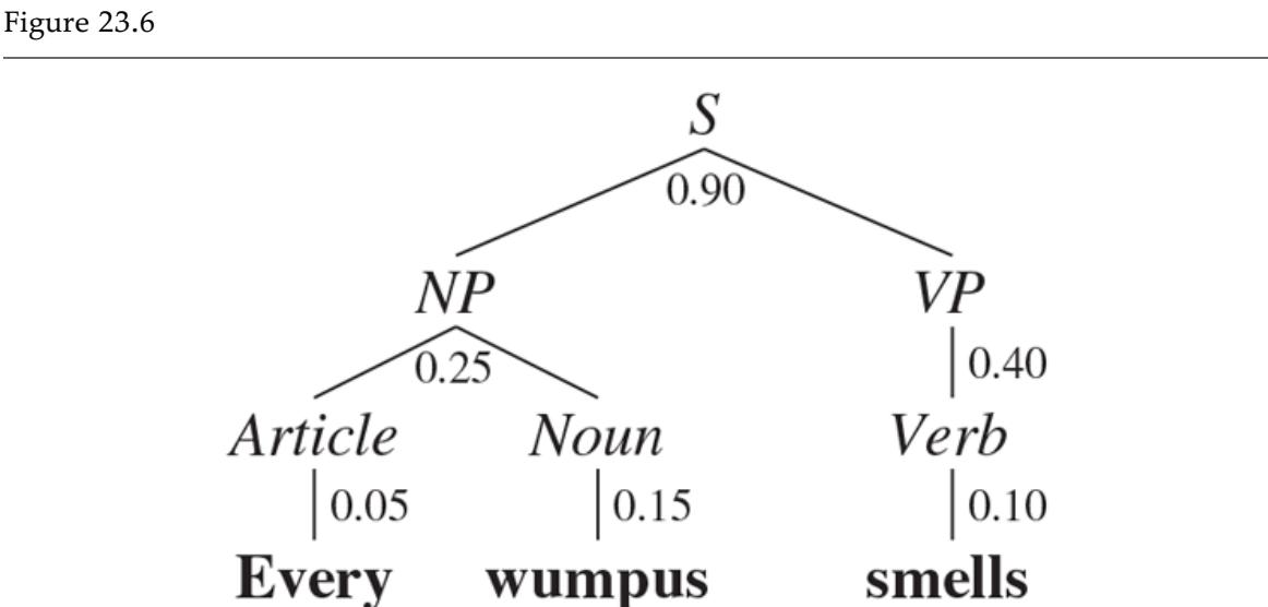
Parse tree for the sentence “Every wumpus smells” according to the grammar Each interior node of the tree is labeled with its probability. The probability of the tree as a whole is The tree can also be written in linear form as

Just as with part-of-speech tagging, we can use a beam search for parsing, where at any time we consider only the most probable alternative parses. This means we are not guaranteed to find the parse with highest probability, but (with a careful implementation) the parser can operate in time and still finds the best parse most of the time.

A beam search parser with is called a deterministic parser. One popular deterministic approach is shift-reduce parsing, in which we go through the sentence word by word, choosing at each point whether to shift the word onto a stack of constituents, or to reduce the top constituent(s) on the stack according to a grammar rule. Each style of parsing has its adherents within the NLP community. Even though it is possible to transform a shift-reduce system into a PCFG (and vice versa), when you apply machine learning to the problem of inducing a grammar, the inductive bias and hence the generalizations that each system will make will be different (Abney et al., 1999).

Deterministic parser

Shift-reduce parsing

23.3.1 Dependency parsing

There is a widely used alternative syntactic approach called dependency grammar, which assumes that syntactic structure is formed by binary relations between lexical items, without a need for syntactic constituents. Figure 23.7 shows a sentence with a dependency parse and a phrase structure parse.

Figure 23.7

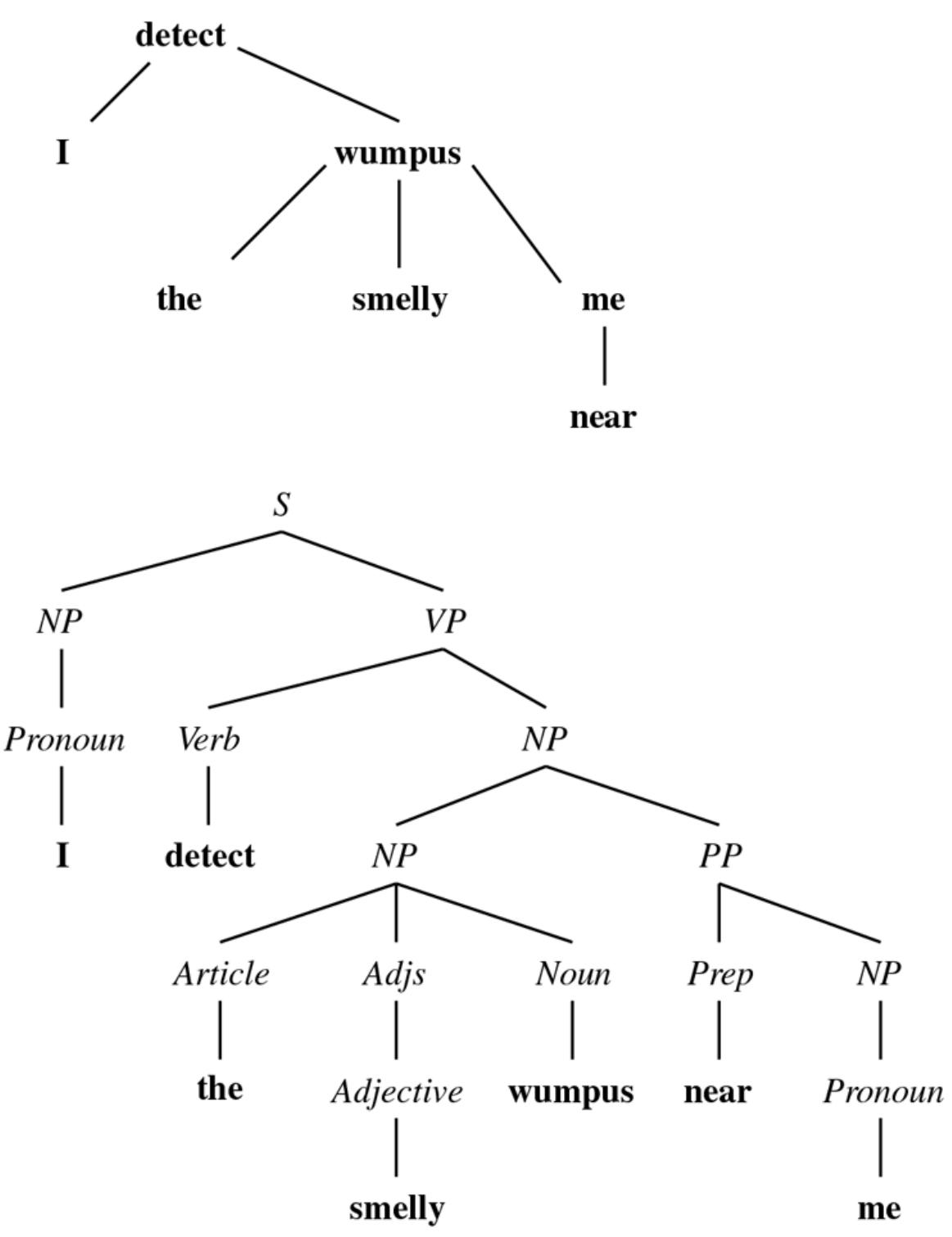
A dependency-style parse (top) and the corresponding phrase structure parse (bottom) for the sentence I detect the smelly wumpus near me.

Dependency grammar

In one sense, dependency grammar and phrase structure grammar are just notational variants. If the phrase structure tree is annotated with the head of each phrase, you can recover the dependency tree from it. In the other direction, we can convert a dependency tree into a phrase structure tree by introducing arbitrary categories (although we might not always get a natural-looking tree this way).

Therefore we wouldn’t prefer one notation over the other because one is more powerful; rather we would prefer one because it is more natural—either more familiar for the human developers of a system, or more natural for a machine learning system which will have to learn the structures. In general, phrase structure trees are natural for languages (like English) with mostly fixed word order; dependency trees are natural for languages (such as Latin) with mostly free word order, where the order of words is determined more by pragmatics than by syntactic categories.

The popularity of dependency grammar today stems in large part from the Universal Dependencies project (Nivre et al., 2016), an open-source treebank project that defines a set of relations and provides millions of parsed sentences in over 70 languages.

23.3.2 Learning a parser from examples

Building a grammar for a significant portion of English is laborious and error prone. This suggests that it would be better to learn the grammar rules (and probabilities) rather than writing them down by hand. To apply supervised learning, we need input/output pairs of sentences and their parse trees. The Penn Treebank is the best known source of such data, with over 100 thousand sentences annotated with parse-tree structure. Figure 23.8 shows an annotated tree from the Penn Treebank.

Figure 23.8

Annotated tree for the sentence “Her eyes were glazed as if she didn’t hear or even see him.” from the Penn Treebank. Note a grammatical phenomenon we have not covered yet: the movement of a phrase from one part of the tree to another. This tree analyzes the phrase “hear or even see him” as consisting of two constituent both of which have a missing object, denoted *-1, which refers to the labeled elsewhere in the tree as [ -1 him]. Similarly, the [ *-2] refers to the [ -2 Her eyes].

Given a treebank, we can create a PCFG just by counting the number of times each nodetype appears in a tree (with the usual caveats about smoothing low counts). In Figure 23.8 , there are two nodes of the form We would count these, and all the other subtrees with root in the corpus. If there are 1000 nodes of which 600 are of this form, then we create the rule:

\[S \to NP\,VP\,\left[0.6\right].\]

All together, the Penn Treebank has over 10,000 different node types. This reflects the fact that English is a complex language, but it also indicates that the annotators who created the treebank favored flat trees, perhaps flatter than we would like. For example, the phrase “the good and the bad” is parsed as a single noun phrase rather than as two conjoined noun phrases, giving us the rule:

There are hundreds of similar rules that define a noun phrase as a string of categories with a conjunction somewhere in the middle; a more concise grammar could capture all the conjoined noun phrase rules with the single rule

\[NP \rightarrow NP \, Conjecture \, NP.\]

Bod et al. (2003) and Bod (2008) show how to automatically recover generalized rules like this, greatly reducing the number of rules that come out of the treebank, and creating a grammar that ends up generalizing better for previously unseen sentences. They call their approach data-oriented parsing.

We have seen that treebanks are not perfect—they contain errors, and have idiosyncratic parses. It is also clear that creating a treebank requires a lot of hard work; that means that treebanks will remain relatively small in size, compared to all the text that has not been annotated with trees. An alternative approach is unsupervised parsing, in which we learn a new grammar (or improve an existing grammar) using a corpus of sentences without trees.

Unsupervised parsing

The inside–outside algorithm (Dodd, 1988), which we will not cover here, learns to estimate the probabilities in a PCFG from example sentences without trees, similar to the way the forward-backward algorithm (Figure 14.4 ) estimates probabilities. Spitkovsky et al. (2010a) describe an unsupervised learning approach that uses curriculum learning: start with the easy part of the curriculum—short unambiguous 2-word sentences like “He left” can be easily parsed based on prior knowledge or annotations. Each new parse of a short sentence extends the system’s knowledge so that it can eventually tackle 3-word, then 4 word, and eventually 40-word sentences.

Curriculum learning

We can also use semisupervised parsing, in which we start with a small number of trees as data to build an initial grammar, then add a large number of unparsed sentences to improve the grammar. The semisupervised approach can make use of partial bracketing: we can use widely available text that has been marked up by the authors, not by linguistic experts, with a partial tree-like structure, in the form of HTML or similar annotations. In HTML text most

brackets correspond to a syntactic component, so partial bracketing can help learn a grammar (Pereira and Schabes, 1992; Spitkovsky et al., 2010b). Consider this HTML text from a newspaper article:

In 1998, however, as I established in The New Republic and Bill Clinton just confirmed in his memoirs, Netanyahu changed his mind

Semisupervised parsing

Partial bracketing

The words surrounded by tags form a noun phrase, and the two strings of words surrounded by tags each form verb phrases.

23.4 Augmented Grammars

So far we have dealt with context-free grammars. But not every can appear in every context with equal probability. The sentence “I ate a banana” is fine, but “Me ate a banana” is ungrammatical, and “I ate a bandanna” is unlikely.

The issue is that our grammar is focused on lexical categories, like Pronoun, but while “I” and “me” are both pronouns, only “I” can be the subject of a sentence. Similarly, “banana” and “bandanna” are both nouns, but the former is much more likely to be object of “ate”. Linguists say that the pronoun “I” is in the subjective case (i.e., is the subject of a verb) and “me” is in the objective case (i.e., is the object of a verb). They also say that “I” is in the first person (“you” is second person, and “she” is third person) and is singular (“we” is plural). A category like Pronoun that has been augmented with features like “subjective case, first person singular” is called a subcategory. 3

3 The subjective case is also sometimes called the nominative case and the objective case is sometimes called the accusative case. Many languages also make another distinction with a dative case for words in the indirect object position.

Subcategory

In this section we show how a grammar can represent this kind of knowledge to make finergrained distinctions about which sentences are more likely. We will also show how to construct a representation of the semantics of a phrase, in a compositional way. All of this will be accomplished with an augmented grammar in which the nonterminals are not just atomic symbols like Pronoun or , but are structured representations. For example, the noun phrase “I” could be represented as which means “a noun phrase that is in the subjective case, first person singular, and whose meaning is the speaker of the sentence.” In contrast, “me” would be represented as marking the fact that it is in the objective case.

Augmented grammar

Consider the sequence “Noun and Noun or Noun,” which can be parsed either as “[Noun and Noun] or Noun,” or as “Noun and [Noun or Noun].” Our context-free grammar has no way to express a preference for one parse over the other, because the rule for conjoined will give the same probability to each parse. We would like a grammar that prefers the parses “[[spaghetti and meatballs] or lasagna]” and “[spaghetti and [pie or cake]]” over the alternative bracketing for each of these phrases.

A lexicalized PCFG is a type of augmented grammar that allows us to assign probabilities based on properties of the words in a phrase other than just the syntactic categories. The data would be very sparse indeed if the probability of, say, a 40-word sentence depended on all 40 words—this is the same problem we noted with n-grams. To simplify, we introduce the notion of the head of a phrase—the most important word. Thus, “banana” is the head of the “a banana” and “ate” is the head of the “ate a banana.” The notation denotes a phrase with category whose head word is Here is a lexicalized PCFG:

VP(v) -> Verb(v) NP(n)	[P1(v,n)
VP(v) -> Verb(v)	P2(v)
NP(n) -> Article(a) Adjs(j) Noun(n)	P3(n,a)
NP(n) -> NP(n) Conjunction(c) NP(m) P4(n,c,m)
Verb(ate) -> ate	0.002
Noun(banana) -> banana	0.0007

Lexicalized PCFG

Head

Here means the probability of a headed by joining with an headed by to form a . We can specify that “ate a banana” is more probable than “ate a bandanna” by ensuring that Note that since we are considering only phrase heads, the distinction between “ate a banana” and “ate a rancid banana” will not be caught by Conceptually, is a huge table of probabilities: if there are 5,000 verbs and 10,000 nouns in the vocabulary, then requires 50 million entries, but most of them will not be stored explicitly; rather they will be derived from smoothing and backoff. For example, we can back off from to a model that depends only on Such a model would require 10,000 times fewer parameters, but can still capture important regularities, such as the fact that a transitive verb like “ate” is more likely to be followed by an (regardless of the head) than an intransitive verb like “sleep.”

We saw in Section 23.2 that the simple grammar for overgenerates, producing nonsentences such as “I saw she” or “I sees her.” To avoid this problem, our grammar would have to know that “her,” not “she,” is a valid object of “saw” (or of any other verb) and that “see,” not “sees,” is the form of the verb that accompanies the subject “I.”

We could encode these facts completely in the probability entries, for example making be a very small number, for all verbs But it is more concise and modular to augment the category with additional variables: is used to represent a noun phrase with case (subjective or objective), person and number (e.g., third person singular), and head noun Figure 23.9 shows an augmented lexicalized grammar that handles these additional variables. Let’s consider one grammar rule in detail:

Figure 23.9

\[\begin{array}{rcl} S(\boldsymbol{\nu}) & \to & NP(Sbj, pn, n) \; VP(pn, \boldsymbol{\nu}) \; | \; \ldots \\ NP(c, pn, n) & \to & Proouon(c, pn, n) \; | \; Nonun(c, pn, n) \; | \; \ldots \\ VP(pn, \boldsymbol{\nu}) & \to & Verb(pn, \boldsymbol{\nu}) \; NP(Obj, pn, n) \; | \; \ldots \\ PP(head) & \to & PP(head) \; NP(Obj, pn, h) \\\\ Pronoun(Sbj, IS, \mathbf{I}) & \to & \mathbf{I} \\ Pronoun(Sbj, IP, \mathbf{w} \mathbf{e}) & \to & \mathbf{w} \mathbf{e} \\ Pronoun(Obj, IS, \mathbf{K}, \mathbf{m} \mathbf{e}) & \to & \mathbf{m} \mathbf{e} \\ Pronun(Obj, 3P, \mathbf{therm}) & \to & \mathbf{then} \\ \end{array}\]

\[\begin{array}{rcl} \text{Verb}(3S, \mathbf{see}) & \to & \mathbf{see} \end{array}\]

Part of an augmented grammar that handles case agreement, subject–verb agreement, and head words. Capitalized names are constants: , and for subjective and objective case; for first person singular; and for first and third person plural. As usual, lowercase names are variables. For simplicity, the probabilities have been omitted.

This rule says that when an NP is followed by a VP they can form an S, but only if the NP has the subjective case and the person and number of the and are identical. (We say that they are in agreement.) If that holds, then we have an whose head is the verb from the . Here is an example lexical rule,

which says that “I” is a Pronoun in the subjective case, first-person singular, with head “I.”

23.4.1 Semantic interpretation

To show how to add semantics to a grammar, we start with an example that is simpler than English: the semantics of arithmetic expressions. Figure 23.10 shows a grammar for arithmetic expressions, where each rule is augmented with a single argument indicating the semantic interpretation of the phrase. The semantics of a digit such as “3” is the digit itself. The semantics of the expression is the operator applied to the semantics of the phrases “3” and “4.” The grammar rules obey the principle of compositional semantics—the semantics of a phrase is a function of the semantics of the subphrases. Figure 23.11 shows the parse tree for according to this grammar. The root of the parse tree is an expression whose semantic interpretation is 5.

\[\begin{array}{l} \operatorname{Exp}(op(\operatorname{x}\_{1},\operatorname{x}\_{2})) \to \operatorname{Exp}(\operatorname{x}\_{1}) \operatorname{Operator}(op)\operatorname{Exp}(\operatorname{x}\_{2})\\ \operatorname{Exp}(\mathbf{x}) \to \{\operatorname{Exp}(\mathbf{x})\} \\ \operatorname{Exp}(\mathbf{x}) \to \operatorname{Number}(\mathbf{x}) \\ \operatorname{Number}(\mathbf{x}) \to \operatorname{Diigit}(\mathbf{x}) \\ \operatorname{Number}(10\times\mathbf{x}\_{1}+\mathbf{x}\_{2}) \to \operatorname{Number}(\mathbf{x}\_{1})\operatorname{Diigit}(\mathbf{x}\_{2}) \\ \operatorname{Operator}(+) \to \cdot \\ \operatorname{Operator}(-) \to \cdot \\ \operatorname{Operator}(\times) \to \times \\ \operatorname{Operator}(\div) \to \div \\ \operatorname{Diigit}(0) \to \mathbf{0} \\ \operatorname{Diigit}(1) \to \mathbf{1} \end{array}\]

A grammar for arithmetic expressions, augmented with semantics. Each variable represents the semantics of a constituent.

Figure 23.11

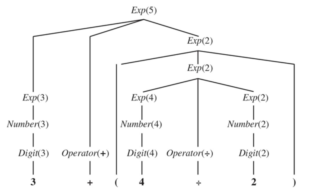
Parse tree with semantic interpretations for the string ” “.

Compositional semantics

Now let’s move on to the semantics of English, or at least a tiny portion of it. We will use first-order logic for our semantic representation. So the simple sentence “Ali loves Bo” should get the semantic representation But what about the constituent phrases? We can represent the “Ali” with the logical term But the “loves Bo” is neither a logical term nor a complete logical sentence. Intuitively, “loves Bo” is a description that might or might not apply to a particular person. (In this case, it applies to Ali.) This means that “loves Bo” is a predicate that, when combined with a term that represents a person, yields a complete logical sentence.

Using the -notation (see page 259), we can represent “loves Bo” as the predicate

Now we need a rule that says “an with semantics followed by a with semantics pred yields a sentence whose semantics is the result of applying pred to n:”

The rule tells us that the semantic interpretation of “Ali loves Bo” is

\[(\lambda x\ Loves(x, Bo))(Ali),\]

which is equivalent to Technically, we say that this is a -reduction of the lambda function application.

The rest of the semantics follows in a straightforward way from the choices we have made so far. Because are represented as predicates, verbs should be predicates as well. The verb “loves” is represented as the predicate that, when given the argument returns the predicate We end up with the grammar and parse tree shown in Figure 23.12 . In a more complete grammar, we would put all the augmentations (semantics, case, person-number, and head) together into one set of rules. Here we show only the semantic augmentation to make it clearer how the rules work.

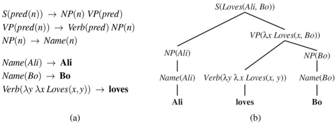
1. A grammar that can derive a parse tree and semantic interpretation for “Ali loves Bo” (and three other sentences). Each category is augmented with a single argument representing the semantics. (b) A parse tree with semantic interpretations for the string “Ali loves Bo.”

23.4.2 Learning semantic grammars

Unfortunately, the Penn Treebank does not include semantic representations of its sentences, just syntactic trees. So if we are going to learn a semantic grammar, we will need a different source of examples. Zettlemoyer and Collins (2005) describe a system that learns a grammar for a question-answering system from examples that consist of a sentence paired with the semantic form for the sentence:

• SENTENCE: What states border Texas?
• LOGICAL FORM:

Given a large collection of pairs like this and a little bit of hand-coded knowledge for each new domain, the system generates plausible lexical entries (for example, that “Texas” and “state” are nouns such that is true), and simultaneously learns parameters for a grammar that allows the system to parse sentences into semantic representations. Zettlemoyer and Collins’s system achieved 79% accuracy on two different test sets of unseen sentences. Zhao and Huang (2015) demonstrate a shift-reduce parser that runs faster, and achieves 85% to 89% accuracy.

A limitation of these systems is that the training data includes logical forms. These are expensive to create, requiring human annotators with specialized expertise—not everyone understands the subtleties of lambda calculus and predicate logic. It is much easier to gather examples of question/answer pairs:

• QUESTION: What states border Texas?
• ANSWER: Louisiana, Arkansas, Oklahoma, New Mexico.
• QUESTION: How many times would Rhode Island fit into California?
• ANSWER: 135

Such question/answer pairs are quite common on the Web, so a large database can be put together without human experts. Using this large source of data it is possible to build parsers that outperform those that use a small database of annotated logical forms (Liang et al., 2011; Liang and Potts, 2015). The key approach described in these papers is to invent an internal logical form that is compositional but does not allow an exponentially large search space.

23.5 Complications of Real Natural Language

The grammar of real English is endlessly complex (and other languages are equally complex). We will briefly mention some of the topics that contribute to this complexity.

QUANTIFICATION: Consider the sentence “Every agent feels a breeze.” The sentence has only one syntactic parse under but it is semantically ambiguous: is there one breeze that is felt by all the agents, or does each agent feel a separate personal breeze? The two interpretations can be represented as

Quantification

One standard approach to quantification is for the grammar to define not an actual logical semantic sentence, but rather a quasi-logical form that is then turned into a logical sentence by algorithms outside of the parsing process. Those algorithms can have preference rules for choosing one quantifier scope over another—preferences that need not be reflected directly in the grammar.

Quasi-logical form

PRAGMATICS: We have shown how an agent can perceive a string of words and use a grammar to derive a set of possible semantic interpretations. Now we address the problem of completing the interpretation by adding context-dependent information about the current situation. The most obvious need for pragmatic information is in resolving the meaning of indexicals, which are phrases that refer directly to the current situation. For example, in the sentence “I am in Boston today,” both “I” and “today” are indexicals. The word “I” would be represented by a fluent that refers to different objects at different times, and it would be up to the hearer to resolve the referent of the fluent—that is not considered part of the grammar but rather an issue of pragmatics.

Pragmatics

Indexical

Another part of pragmatics is interpreting the speaker’s intent. The speaker’s utterance is considered a speech act, and it is up to the hearer to decipher what type of action it is—a question, a statement, a promise, a warning, a command, and so on. A command such as “go to 2 2” implicitly refers to the hearer. So far, our grammar for covers only declarative sentences. We can extend it to cover commands—a command is a verb phrase where the subject is implicitly the hearer of the command:

Speech act

LONG-DISTANCE DEPENDENCIES: In Figure 23.8 we saw that “she didn’t hear or even see him” was parsed with two gaps where an is missing, but refers to the “him.” We can use the symbol to represent the gaps: “she didn’t [hear or even see ] him.” In general, the distance between the gap and the it refers to can be arbitrarily long: in

“Who did the agent tell you to give the gold to ?” the gap refers to “Who,” which is 11 words away.

Long-distance dependencies

A complex system of augmented rules can be used to make sure that the missing s match up properly. The rules are complex; for example, you can’t have a gap in one branch of an conjunction: “What did she play [ Dungeons and ]?” is ungrammatical. But you can have the same gap in both branches of a conjunction, as in the sentence “What did you [ [ smell ] and [ shoot an arrow at ]]?”

TIME AND TENSE: Suppose we want to represent the difference between “Ali loves Bo” and “Ali loved Bo.” English uses verb tenses (past, present, and future) to indicate the relative time of an event. One good choice to represent the time of events is the event calculus notation of Section 10.3 . In event calculus we have

Time and tense

This suggests that our two lexical rules for the words “loves” and “loved” should be these:

Other than this change, everything else about the grammar remains the same, which is encouraging news; it suggests we are on the right track if we can so easily add a complication like the tense of verbs (although we have just scratched the surface of a complete grammar for time and tense).

Ambiguity: We tend to think of ambiguity as a failure in communication; when a listener is consciously aware of an ambiguity in an utterance, it means that the utterance is unclear or confusing. Here are some examples taken from newspaper headlines:

Squad helps dog bite victim.

Police begin campaign to run down jaywalkers.

Helicopter powered by human flies.

Once-sagging cloth diaper industry saved by full dumps.

Include your children when baking cookies.

Portable toilet bombed; police have nothing to go on.

Milk drinkers are turning to powder.

Two sisters reunited after 18 years in checkout counter.

Such confusions are the exception; most of the time the language we hear seems unambiguous. Thus, when researchers first began to use computers to analyze language in the 1960s, they were quite surprised to learn that almost every sentence is ambiguous, with multiple possible parses (sometimes hundreds), even when the single preferred parse is the only one that native speakers notice. For example, we understand the phrase “brown rice and black beans” as “[brown rice] and [black beans],” and never consider the lowprobability interpretation “brown [rice and black beans],” where the adjective “brown” is modifying the whole phrase, not just the “rice.” When we hear “Outside of a dog, a book is a person’s best friend,” we interpret “outside of” as meaning “except for,” and find it funny when the next sentence of the Groucho Marx joke is “Inside of a dog it’s too dark to read.”

Lexical ambiguity is when a word has more than one meaning: “back” can be an adverb (go back), an adjective (back door), a noun (the back of the room), a verb (back a candidate), or a proper noun (a river in Nunavut, Canada). “Jack” can be a proper name, a noun (a playing card, a six-pointed metal game piece, a nautical flag, a fish, a bird, a cheese, a socket, etc.), or a verb (to jack up a car, to hunt with a light, or to hit a baseball hard). Syntactic

ambiguity refers to a phrase that has multiple parses: “I smelled a wumpus in 2,2” has two parses: one where the prepositional phrase “in 2,2” modifies the noun and one where it modifies the verb. The syntactic ambiguity leads to a semantic ambiguity, because one parse means that the wumpus is in 2,2 and the other means that a stench is in 2,2. In this case, getting the wrong interpretation could be a deadly mistake.

Lexical ambiguity

Syntactic ambiguity

Semantic ambiguity

There can also be ambiguity between literal and figurative meanings. Figures of speech are important in poetry, and are common in everyday speech as well. A metonymy is a figure of speech in which one object is used to stand for another. When we hear “Chrysler announced a new model,” we do not interpret it as saying that companies can talk; rather we understand that a spokesperson for the company made the announcement. Metonymy is common and is often interpreted unconsciously by human hearers.

Metonymy

Unfortunately, our grammar as it is written is not so facile. To handle the semantics of metonymy properly, we need to introduce a whole new level of ambiguity. We could do this by providing two objects for the semantic interpretation of every phrase in the sentence: one for the object that the phrase literally refers to (Chrysler) and one for the metonymic

reference (the spokesperson). We then have to say that there is a relation between the two. In our current grammar, “Chrysler announced” gets interpreted as

\[x = Chrysler \land e \in Announce(x) \land After(Now, Extract(e)).\]

We need to change that to

\[x = Chrysler \land e \in Announce(m) \land After(Now, Extract(e))\]

\[\land Metonymy \, (m, x).\]

This says that there is one entity that is equal to Chrysler, and another entity that did the announcing, and that the two are in a metonymy relation. The next step is to define what kinds of metonymy relations can occur. The simplest case is when there is no metonymy at all—the literal object and the metonymic object are identical:

\[ \forall m, x \; (m = x) \Rightarrow Metong \\ my(m, x). \]

For the Chrysler example, a reasonable generalization is that an organization can be used to stand for a spokesperson of that organization:

\[ \forall m, x \; x \in Organizations \land Spokesperson(m, x) \Rightarrow Metongmy(m, x). \]

Other metonymies include the author for the works (I read Shakespeare) or more generally the producer for the product (I drive a Honda) and the part for the whole (The Red Sox need a strong arm). Some examples of metonymy, such as “The ham sandwich on Table 4 wants another beer,” are more novel and are interpreted with respect to a situation (such as waiting on tables and not knowing a customer’s name).

A metaphor is another figure of speech, in which a phrase with one literal meaning is used to suggest a different meaning by way of an analogy. Thus, metaphor can be seen as a kind of metonymy where the relation is one of similarity.

Metaphor

Disambiguation

Disambiguation is the process of recovering the most probable intended meaning of an utterance. In one sense we already have a framework for solving this problem: each rule has a probability associated with it, so the probability of an interpretation is the product of the probabilities of the rules that led to the interpretation. Unfortunately, the probabilities reflect how common the phrases are in the corpus from which the grammar was learned, and thus reflect general knowledge, not specific knowledge of the current situation. To do disambiguation properly, we need to combine four models:

• 1. The world model: the likelihood that a proposition occurs in the world. Given what we know about the world, it is more likely that a speaker who says “I’m dead” means “I am in big trouble” or “I lost this video game” rather than “My life ended, and yet I can still talk.”
• 2. The mental model: the likelihood that the speaker forms the intention of communicating a certain fact to the hearer. This approach combines models of what the speaker believes, what the speaker believes the hearer believes, and so on. For example, when a politician says, “I am not a crook,” the world model might assign a probability of only 50% to the proposition that the politician is not a criminal, and 99.999% to the proposition that he is not a hooked shepherd’s staff. Nevertheless, we select the former interpretation because it is a more likely thing to say.
• 3. The language model: the likelihood that a certain string of words will be chosen, given that the speaker has the intention of communicating a certain fact.
• 4. The acoustic model: for spoken communication, the likelihood that a particular sequence of sounds will be generated, given that the speaker has chosen a given string of words. (For handwritten or typed communication, we have the problem of optical character recognition.)

23.6 Natural Language Tasks

Natural language processing is a big field, deserving an entire textbook or two of its own (Goldberg, 2017; Jurafsky and Martin, 2020). In this section we briefly describe some of the main tasks; you can use the references to get more details.

Speech recognition is the task of transforming spoken sound into text. We can then perform further tasks (such as question answering) on the resulting text. Current systems have a word error rate of about 3% to 5% (depending on details of the test set), similar to human transcribers. The challenge for a system using speech recognition is to respond appropriately even when there are errors on individual words.

Speech recognition

Top systems today use a combination of recurrent neural networks and hidden Markov models (Hinton et al., 2012; Yu and Deng, 2016; Deng, 2016; Chiu et al., 2017; Zhang et al., 2017). The introduction of deep neural nets for speech in 2011 led to an immediate and dramatic improvement of about 30% in error rate—this from a field that seemed to be mature and was previously progressing at only a few percent per year. Deep neural networks are a good fit because the problem of speech recognition has a natural compositional breakdown: waveforms to phonemes to words to sentences. They will be covered in the next chapter.

Text-to-speech synthesis is the inverse process—going from text to sound. Taylor (2009) gives a book-length overview. The challenge is to pronounce each word correctly, and to make the flow of each sentence seem natural, with the right pauses and emphasis.

Text-to-speech

Another area of development is in synthesizing different voices—starting with a choice between a generic male or female voice, then allowing for regional dialects, and even imitating celebrity voices. As with speech recognition, the introduction of deep recurrent neural networks led to a large improvement, with about 2/3 of listeners saying that the neural WaveNet system (van den Oord et al., 2016a) sounded more natural than the previous non-neural system.

Machine translation transforms text in one language to another. Systems are usually trained using a bilingual corpus: a set of paired documents, where one member of the pair is in, say, English, and the other is in, say, French. The documents do not need to be annotated in any way; the machine translation system learns to align sentences and phrases and then when presented with a novel sentence in one language, can generate a translation to the other.

Systems in the early 2000s used -gram models, and achieved results that were usually good enough to get across the meaning of a text, but contained syntactic errors in most sentences. One problem was the limit on the length of the -grams: even with a large limit of 7, it was difficult for information to flow from one end of the sentence to the other. Another problem was that all the information in an -gram model is at the level of individual words. Such a system could learn that “black cat” translates to “chat noir,” but it could not learn the rule that adjectives generally come before the noun in English and after the noun in French.

Recurrent neural sequence-to-sequence models (Sutskever et al., 2015) got around the problem. They could generalize better (because they could use word embeddings rather than -gram counts of specific words) and could form compositional models throughout the various levels of the deep network to effectively pass information along. Subsequent work using the attention-focusing mechanism of the transformer model (Vaswani et al., 2018) increased performance further, and a hybrid model incorporating aspects of both these models does better still, approaching human-level performance on some language pairs (Wu et al., 2016b; Chen et al., 2018).

Information extraction is the process of acquiring knowledge by skimming a text and looking for occurrences of particular classes of objects and for relationships among them. A typical task is to extract instances of addresses from Web pages, with database fields for street, city, state, and zip code; or instances of storms from weather reports, with fields for

temperature, wind speed, and precipitation. If the source text is well structured (for example, in the form of a table), then simple techniques such as regular expressions can extract the information (Cafarella et al., 2008). It gets harder if we are trying to extract all facts, rather than a specific type (such as weather reports); Banko et al. (2007) describe the TEXTRUNNER system that performs extraction over an open, expanding set of relations. For free-form text, techniques include hidden Markov models and rule-based learning systems (as used in TEXTRUNNER and NELL (Never-Ending Language Learning) (Mitchell et al., 2018)). More recent systems use recurrent neural networks, taking advantage of the flexibility of word embeddings. You can find an overview in Kumar (2017).

Information extraction

Information retrieval is the task of finding documents that are relevant and important for a given query. Internet search engines such as Google and Baidu perform this task billions of times a day. Three good textbooks on the subject are Manning et al. (2008), Croft et al. (2010), and Baeza-Yates and Ribeiro-Neto (2011).

Information retrieval

Question Answering is a different task, in which the query really is a question, such as “Who founded the U.S. Coast Guard?” and the response is not a ranked list of documents but rather an actual answer: “Alexander Hamilton.” There have been question-answering systems since the 1960s that rely on syntactic parsing as discussed in this chapter, but only since 2001 have such systems used Web information retrieval to radically increase their breadth of coverage. Katz (1997) describes the START parser and question answerer. Banko et al. (2002) describe ASKMSR, which was less sophisticated in terms of its syntactic parsing ability, but more aggressive in using Web search and sorting through the results. For example, to answer “Who founded the U.S. Coast Guard?” it would search for queries such as [* founded the U.S. Coast Guard] and [the U.S. Coast Guard was founded by *], and

then examine the multiple resulting Web pages to pick out a likely response, knowing that the query word “who” suggests that the answer should be a person. The Text REtrieval Conference (TREC) gathers research on this topic and has hosted competitions on an annual basis since 1991 (Allan et al., 2017). Recently we have seen other test sets, such as the AI2 ARC test set of basic science questions (Clark et al., 2018).

Question Answering

Summary

The main points of this chapter are as follows:

• Probabilistic language models based on -grams recover a surprising amount of information about a language. They can perform well on such diverse tasks as language identification, spelling correction, sentiment analysis, genre classification, and namedentity recognition.
• These language models can have millions of features, so preprocessing and smoothing the data to reduce noise is important.
• In building a statistical language system, it is best to devise a model that can make good use of available data, even if the model seems overly simplistic.
• Word embeddings can give a richer representation of words and their similarities.
• To capture the hierarchical structure of language, phrase structure grammars (and in particular, context-free grammars) are useful. The probabilistic context-free grammar (PCFG) formalism is widely used, as is the dependency grammar formalism.
• Sentences in a context-free language can be parsed in time by a chart parser such as the CYK algorithm, which requires grammar rules to be in Chomsky Normal Form. With a small loss in accuracy, natural languages can be parsed in time, using a beam search or a shift-reduce parser.
• A treebank can be a resource for learning a PCFG grammar with parameters.
• It is convenient to augment a grammar to handle issues such as subject–verb agreement and pronoun case, and to represent information at the level of words rather than just at the level of categories.
• Semantic interpretation can also be handled by an augmented grammar. We can learn a semantic grammar from a corpus of questions paired either with the logical form of the question, or with the answer.
• Natural language is complex and difficult to capture in a formal grammar.

Bibliographical and Historical Notes

-gram letter models for language modeling were proposed by Markov (1913). Claude Shannon (Shannon and Weaver, 1949) was the first to generate -gram word models of English. The bag-of-words model gets its name from a passage from linguist Zellig Harris (1954), “language is not merely a bag of words but a tool with particular properties.” Norvig (2009) gives some examples of tasks that can be accomplished with -gram models.

Chomsky (1956, 1957) pointed out the limitations of finite-state models compared with context-free models, concluding, “Probabilistic models give no particular insight into some of the basic problems of syntactic structure.” This is true, but probabilistic models do provide insight into some other basic problems—problems that context-free models ignore. Chomsky’s remarks had the unfortunate effect of scaring many people away from statistical models for two decades, until these models reemerged for use in the field of speech recognition (Jelinek, 1976), and in cognitive science, where optimality theory (Smolensky and Prince, 1993; Kager, 1999) posited that language works by finding the most probable candidate that optimally satisfies competing constraints.

Add-one smoothing, first suggested by Pierre-Simon Laplace (1816), was formalized by Jeffreys (1948). Other smoothing techniques include interpolation smoothing (Jelinek and Mercer, 1980), Witten–Bell smoothing (1991), Good–Turing smoothing (Church and Gale, 1991), Kneser–Ney smoothing (1995, 2004), and stupid backoff (Brants et al., 2007). Chen and Goodman (1996) and Goodman (2001) survey smoothing techniques.

Simple -gram letter and word models are not the only possible probabilistic models. The latent Dirichlet allocation model (Blei et al., 2002; Hoffman et al., 2011) is a probabilistic text model that views a document as a mixture of topics, each with its own distribution of words. This model can be seen as an extension and rationalization of the latent semantic indexing model of Deerwester et al. (1990) and is also related to the multiple-cause mixture model of (Sahami et al., 1996). And of course there is great interest in non-probabilistic language models, such as the deep learning models covered in Chapter 24 .

Joulin et al. (2016) give a bag of tricks for efficient text classification. Joachims (2001) uses statistical learning theory and support vector machines to give a theoretical analysis of when classification will be successful. Apté et al. (1994) report an accuracy of 96% in classifying Reuters news articles into the “Earnings” category. Koller and Sahami (1997) report accuracy up to 95% with a naive Bayes classifier, and up to 98.6% with a Bayes classifier.

Schapire and Singer (2000) show that simple linear classifiers can often achieve accuracy almost as good as more complex models, and run faster. Zhang et al. (2016) describe a character-level (rather than word-level) text classifier. Witten et al. (1999) describe compression algorithms for classification, and show the deep connection between the LZW compression algorithm and maximum-entropy language models.

Wordnet (Fellbaum, 2001) is a publicly available dictionary of about 100,000 words and phrases, categorized into parts of speech and linked by semantic relations such as synonym, antonym, and part-of. Charniak (1996) and Klein and Manning (2001) discuss parsing with treebank grammars. The British National Corpus (Leech et al., 2001) contains 100 million words, and the World Wide Web contains several trillion words; Franz and Brants (2006) describe the publicly available Google -gram corpus of 13 million unique words from a trillion words of Web text. Buck et al. (2014) describe a similar data set from the Common Crawl project. The Penn Treebank (Marcus et al., 1993; Bies et al., 2015) provides parse trees for a 3-million-word corpus of English.

Many of the -gram model techniques are also used in bioinformatics problems. Biostatistics and probabilistic NLP are coming closer together, as each deals with long, structured sequences chosen from an alphabet.

Early part-of-speech (POS) taggers used a variety of techniques, including rule sets (Brill, 1992), -grams (Church, 1988), decision trees (Màrquez and Rodrí guez, 1998), HMMs (Brants, 2000), and logistic regression (Ratnaparkhi, 1996). Historically, a logistic regression model was also called a “maximum entropy Markov model” or MEMM, so some work is under that name. Jurafsky and Martin (2020) have a good chapter on POS tagging. Ng and Jordan (2002) compare discriminative and generative models for classification tasks.

Like semantic networks, context-free grammars were first discovered by ancient Indian grammarians (especially Panini, ca. 350 BCE) studying Shastric Sanskrit (Ingerman, 1967). They were reinvented by Noam Chomsky (1956) for the analysis of English and independently by John Backus (1959) and Peter Naur for the analysis of Algol-58.

Probabilistic context-free grammars were first investigated by Booth (1969) and Salomaa (1969). Algorithms for PCFGs are presented in the excellent short monograph by Charniak (1993) and the excellent long textbooks by Manning and Schütze (1999) and Jurafsky and Martin (2020). Baker (1979) introduces the inside–outside algorithm for learning a PCFG. Lexicalized PCFGs (Charniak, 1997; Hwa, 1998) combine the best aspects of PCFGs and gram models. Collins (1999) describes PCFG parsing that is lexicalized with head features, and Johnson (1998) shows how the accuracy of a PCFG depends on the structure of the treebank from which its probabilities were learned.

There have been many attempts to write formal grammars of natural languages, both in “pure” linguistics and in computational linguistics. There are several comprehensive but informal grammars of English (Quirk et al., 1985; McCawley, 1988; Huddleston and Pullum, 2002). Since the 1980s, there has been a trend toward lexicalization: putting more information in the lexicon and less in the grammar.

Lexical-functional grammar, or LFG (Bresnan, 1982) was the first major grammar formalism to be highly lexicalized. If we carry lexicalization to an extreme, we end up with categorial grammar (Clark and Curran, 2004), in which there can be as few as two grammar rules, or with dependency grammar (Smith and Eisner, 2008; Kübler et al., 2009) in which there are no syntactic categories, only relations between words.

Computerized parsing was first demonstrated by Yngve (1955). Efficient algorithms were developed in the 1960s, with a few twists since then (Kasami, 1965; Younger, 1967; Earley, 1970; Graham et al., 1980). Church and Patil (1982) describe syntactic ambiguity and address ways to resolve it.

Klein and Manning (2003) describe A* parsing, and Pauls and Klein (2009) extend that to Kbest A* parsing, in which the result is not a single parse but the best. Goldberg et al. (2013) describe the necessary implementation tricks to make sure that a beam search parser is and not Zhu et al. (2013) describe a fast deterministic shift-reduce parser for natural languages, and Sagae and Lavie (2006) show how adding search to a shift-reduce parser can make it more accurate, at the cost of some speed.

Today, highly accurate open-source parsers include Google’s Parsey McParseface (Andor et al., 2016), the Stanford Parser (Chen and Manning, 2014), the Berkeley Parser (Kitaev and

Klein, 2018), and the SPACY parser. They all do generalization through neural networks and achieve roughly 95% accuracy on Wall Street Journal or Penn Treebank test sets. There is some criticism of the field that it is focusing too narrowly on measuring performance on a few select corpora, and perhaps overfitting on them.

Formal semantic interpretation of natural languages originates within philosophy and formal logic, particularly Alfred Tarski’s (1935) work on the semantics of formal languages. Bar-Hillel (1954) was the first to consider the problems of pragmatics (such as indexicals) and propose that they could be handled by formal logic. Richard Montague’s essay “English as a formal language” (1970) is a kind of manifesto for the logical analysis of language, but there are other books that are more readable (Dowty et al., 1991; Portner and Partee, 2002; Cruse, 2011). While semantic interpretation programs are designed to pick the most likely interpretation, literary critics (Empson, 1953; Hobbs, 1990) have been ambiguous about whether ambiguity is something to be resolved or cherished. Norvig (1988) discusses the problems of considering multiple simultaneous interpretations, rather than settling for a single maximum-likelihood interpretation. Lakoff and Johnson (1980) give an engaging analysis and catalog of common metaphors in English. Martin (1990) and Gibbs (2006) offer computational models of metaphor interpretation.

The first NLP system to solve an actual task was the BASEBALL question answering system (Green et al., 1961), which handled questions about a database of baseball statistics. Close after that was Winograd’s (1972) SHRDLU, which handled questions and commands about a blocks-world scene, and Woods’s (1973) LUNAR, which answered questions about the rocks brought back from the moon by the Apollo program.

Banko et al. (2002) present the ASKMSR question-answering system; a similar system is due to Kwok et al. (2001). Pasca and Harabagiu (2001) discuss a contest-winning questionanswering system.

Modern approaches to semantic interpretation usually assume that the mapping from syntax to semantics will be learned from examples (Zelle and Mooney, 1996; Zettlemoyer and Collins, 2005; Zhao and Huang, 2015). The first important result on grammar induction was a negative one: Gold (1967) showed that it is not possible to reliably learn an exactly correct context-free grammar, given a set of strings from that grammar. Prominent linguists, such as Chomsky (1957) and Pinker (2003), have used Gold’s result to argue that there must

be an innate universal grammar that all children have from birth. The so-called Poverty of the Stimulus argument says that children aren’t given enough input to learn a CFG, so they must already “know” the grammar and be merely tuning some of its parameters.

Universal grammar

While this argument continues to hold sway throughout much of Chomskyan linguistics, it has been dismissed by other linguists (Pullum, 1996; Elman et al., 1997) and most computer scientists. As early as 1969, Horning showed that it is possible to learn, in the sense of PAC learning, a probabilistic context-free grammar. Since then, there have been many convincing empirical demonstrations of language learning from positive examples alone, such as learning semantic grammars with inductive logic programming (Muggleton and De Raedt, 1994; Mooney, 1999), the Ph.D. theses of Schütze (1995) and de Marcken (1996), and the entire line of modern language processing systems based on the transformer model (Section 24). There is an annual International Conference on Grammatical Inference (ICGI).

James Baker’s DRAGON system (Baker, 1975) could be considered the first succesful speech recognition system. It was the first to use HMMs for speech. After several decades of systems based on probabilistic language models, the field began to switch to deep neural networks (Hinton et al., 2012). Deng (2016) describes how the introduction of deep learning enabled rapid improvement in speech recognition, and reflects on the implications for other NLP tasks. Today deep learning is the dominant approach for all large-scale speech recognition systems. Speech recognition can be seen as the first application area that highlighted the success of deep learning, with computer vision following shortly thereafter.

Interest in the field of information retrieval was spurred by widespread usage of Internet searching. Croft et al. (2010) and Manning et al. (2008) provide textbooks that cover the basics. The TREC conference hosts an annual competition for IR systems and publishes proceedings with results.

Brin and Page (1998) describe the PageRank algorithm, which takes into account the links between pages, and give an overview of the implementation of a Web search engine.

Silverstein et al. (1998) investigate a log of a billion Web searches. The journal Information Retrieval and the proceedings of the annual flagship SIGIR conference cover recent developments in the field.

Information extraction has been pushed forward by the annual Message Understanding Conferences (MUC), sponsored by the U.S. government. Surveys of template-based systems are given by Roche and Schabes (1997), Appelt (1999), and Muslea (1999). Large databases of facts were extracted by Craven et al. (2000), Pasca et al. (2006), Mitchell (2007), and Durme and Pasca (2008). Freitag and McCallum (2000) discuss HMMs for Information Extraction. Conditional random fields have also been used for this task (Lafferty et al., 2001; McCallum, 2003); a tutorial with practical guidance is given by Sutton and McCallum (2007). Sarawagi (2007) gives a comprehensive survey.

Two early influential approaches to automated knowledge engineering for NLP were by Riloff (1993), who showed that an automatically constructed dictionary performed almost as well as a carefully handcrafted domain-specific dictionary, and by Yarowsky (1995), who showed that the task of word sense classification could be accomplished through unsupervised training on a corpus of unlabeled text with accuracy as good as supervised methods.

The idea of simultaneously extracting templates and examples from a handful of labeled examples was developed independently and simultaneously by Blum and Mitchell (1998), who called it cotraining, and by Brin (1998), who called it DIPRE (Dual Iterative Pattern Relation Extraction). You can see why the term cotraining has stuck. Similar early work, under the name of bootstrapping, was done by Jones et al. (1999). The method was advanced by the QXTRACT (Agichtein and Gravano, 2003) and KNOWITALL (Etzioni et al., 2005) systems. Machine reading was introduced by Mitchell (2005) and Etzioni et al. (2006) and is the focus of the TEXTRUNNER project (Banko et al., 2007; Banko and Etzioni, 2008).

This chapter has focused on natural language sentences, but it is also possible to do information extraction based on the physical structure or geometric layout of text rather than on the linguistic structure. Lists, tables, charts, graphs, diagrams, etc., whether encoded in HTML or accessed through the visual analysis of pdf documents, are home to data that can be extracted and consolidated (Hurst, 2000; Pinto et al., 2003; Cafarella et al., 2008).

Ken Church (2004) shows that natural language research has cycled between concentrating on the data (empiricism) and concentrating on theories (rationalism); he describes the advantages of having good language resources and evaluation schemes, but wonders if we have gone too far (Church and Hestness, 2019). Early linguists concentrated on actual language usage data, including frequency counts. Noam Chomsky (1956) demonstrated the limitations of finite-state models, leading to an emphasis on theoretical studies of syntax, disregarding actual language performance. This approach dominated for twenty years, until empiricism made a comeback based on the success of work in statistical speech recognition (Jelinek, 1976). Today, the emphasis on empirical language data continues, and there is heightened interest in models that consider higher-level constructs, such as syntactic and semantic relations, not just sequences of words. There is also a strong emphasis on deep learning neural network models of language, which we will cover in Chapter 24 .

Work on applications of language processing is presented at the biennial Applied Natural Language Processing conference (ANLP), the conference on Empirical Methods in Natural Language Processing (EMNLP), and the journal Natural Language Engineering. A broad range of NLP work appears in the journal Computational Linguistics and its conference, ACL, and in the International Computational Linguistics (COLING) conference. Jurafsky and Martin (2020) give a comprehensive introduction to speech and NLP.

Chapter 24 Deep Learning for Natural Language Processing

In which deep neural networks perform a variety of language tasks, capturing the structure of natural language as well as its fluidity.

Chapter 23 explained the key elements of natural language, including grammar and semantics. Systems based on parsing and semantic analysis have demonstrated success on many tasks, but their performance is limited by the endless complexity of linguistic phenomena in real text. Given the vast amount of text available in machine-readable form, it makes sense to consider whether approaches based on data-driven machine learning can be more effective. We explore this hypothesis using the tools provided by deep learning systems (Chapter 21 ).

We begin in Section 24.1 by showing how learning can be improved by representing words as points in a high-dimensional space, rather than as atomic values. Section 24.2 covers the use of recurrent neural networks to capture meaning and long-distance context as text is processed sequentially. Section 24.3 focuses primarily on machine translation, one of the major successes of deep learning applied to NLP. Sections 24.4 and 24.5 cover models that can be trained from large amounts of unlabeled text and then applied to specific tasks, often achieving state-of-the-art performance. Finally, Section 24.6 takes stock of where we are and how the field may progress.

24.1 Word Embeddings

We would like a representation of words that does not require manual feature engineering, but allows for generalization between related words—words that are related syntactically (“colorless” and “ideal” are both adjectives), semantically (“cat” and “kitten” are both felines), topically (“sunny” and “sleet” are both weather terms), in terms of sentiment (“awesome” has opposite sentiment to “cringeworthy”), or otherwise.

How should we encode a word into an input vector for use in a neural network? As explained in Section 21.2.1 (page 756), we could use a one-hot vector—that is, we encode the th word in the dictionary with a 1 bit in the th input position and a 0 in all the other positions. But such a representation would not capture the similarity between words.

Following the linguist John R. Firth’s (1957) maxim, “You shall know a word by the company it keeps,” we could represent each word with a vector of -gram counts of all the phrases that the word appears in. However, raw -gram counts are cumbersome. With a 100,000-word vocabulary, there are 5-grams to keep track of (although vectors in this -dimensional space would be quite sparse—most of the counts would be zero). We would get better generalization if we reduced this to a smaller-size vector, perhaps with just a few hundred dimensions. We call this smaller, dense vector a word embedding: a lowdimensional vector representing a word. Word embeddings are learned automatically from the data. (We will see later how this is done.) What are these learned word embeddings like? On the one hand, each one is just a vector of numbers, where the individual dimensions and their numeric values do not have discernible meanings:

Word embedding

On the other hand, the feature space has the property that similar words end up having similar vectors. We can see that in Figure 24.1 , where there are separate clusters for country, kinship, transportation, and food words.

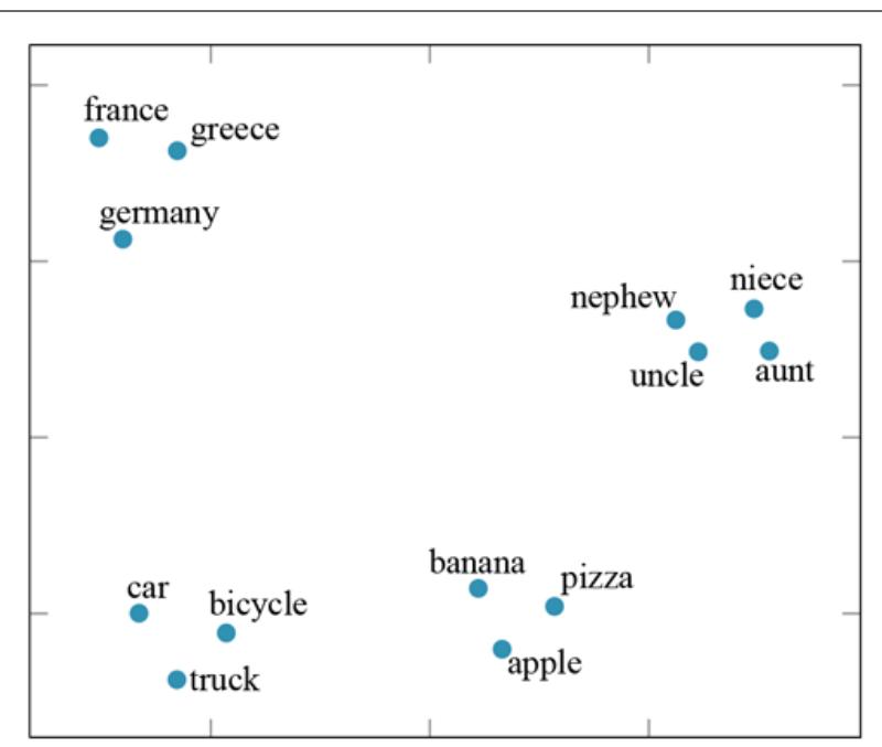
Figure 24.1

Word embedding vectors computed by the GloVe algorithm trained on 6 billion words of text. 100 dimensional word vectors are projected down onto two dimensions in this visualization. Similar words appear near each other.

It turns out, for reasons we do not completely understand, that the word embedding vectors have additional properties beyond mere proximity for similar words. For example, suppose we look at the vectors for Athens and for Greece. For these words the vector difference seems to encode the country/capital relationship. Other pairs—France and Paris, Russia and Moscow, Zambia and Lusaka—have essentially the same vector difference.

We can use this property to solve word analogy problems such as “Athens is to Greece as Oslo is to [what]?” Writing for the Oslo vector and for the unknown, we hypothesize that , giving us . And when we compute this new vector , we find that it is closer to “Norway” than to any other word. Figure 24.2 shows that this type of vector arithmetic works for many relationships.

A	B	C	D=C+(B-A)	Relationship
Athens	Greece	Oslo	Norway	Capital
Astana	Kazakhstan	Harare	Zimbabwe	Capital
Angola	kwanza	Iran	rial	Currency
copper	Cu	gold	Au	Atomic Symbol
Microsoft	Windows	Google	Android	Operating System
New York	New York Times	Baltimore	Baltimore Sun	Newspaper
Berlusconi	Silvio	Obama	Barack	First name
Switzerland	Swiss	Cambodia	Cambodian	Nationality
Einstein	scientist	Picasso	painter	Occupation
brother	sister	grandson	granddaughter	Family Relation
Chicago	Illinois	Stockton	California	State
possibly	impossibly	ethical	unethical	Negative
mouse	mice	dollar	dollars	Plural
easy	easiest	lucky	luckiest	Superlative
walking	walked	swimming	swam	Past tense

A word embedding model can sometimes answer the question ” is to as is to [what]?” with vector arithmetic: given the word embedding vectors for the words , , and , compute the vector and look up the word that is closest to . (The answers in column were computed automatically by the model. The descriptions in the “Relationship” column were added by hand.) Adapted from Mikolov et al. (2013, 2014).

However, there is no guarantee that a particular word embedding algorithm run on a particular corpus will capture a particular semantic relationship. Word embeddings are popular because they have proven to be a good representation for downstream language tasks (such as question answering or translation or summarization), not because they are guaranteed to answer analogy questions on their own.

Using word embedding vectors rather than one-hot encodings of words turns out to be helpful for essentially all applications of deep learning to NLP tasks. Indeed, in many cases it is possible to use generic pretrained vectors, obtained from any of several suppliers, for one’s particular NLP task. At the time of writing, the commonly used vector dictionaries include WORD2VEC, GloVe (Global Vectors), and FASTTEXT, which has embeddings for 157 languages. Using a pretrained model can save a great deal of time and effort. For more on these resources, see Section 24.5.1 .

It is also possible to train your own word vectors; this is usually done at the same time as training a network for a particular task. Unlike generic pretrained embeddings, word embeddings produced for a specific task can be trained on a carefully selected corpus and will tend to emphasize aspects of words that are useful for the task. Suppose, for example, that the task is part-of-speech (POS) tagging (see Section 23.1.6 ). Recall that this involves predicting the correct part of speech for each word in a sentence. Although this is a simple task, it is nontrivial because many words can be tagged in multiple ways—for example, the word cut can be a present-tense verb (transitive or intransitive), a past-tense verb, an infinitive verb, a past participle, an adjective, or a noun. If a nearby temporal adverb refers to the past, that suggests that this particular occurrence of cut is a past-tense verb; and we might hope, then, that the embedding will capture the past-referring aspect of adverbs.

POS tagging serves as a good introduction to the application of deep learning to NLP, without the complications of more complex tasks like question answering (see Section 24.5.3 ). Given a corpus of sentences with POS tags, we learn the parameters for the word embeddings and the POS tagger simultaneously. The process works as follows:

• 1. Choose the width (an odd number of words) for the prediction window to be used to tag each word. A typical value is , meaning that the tag is predicted based on the word plus the two words to the left and the two words to the right. Split every sentence in your corpus into overlapping windows of length . Each window produces one training example consisting of the words as input and the POS category of the middle word as output.
• 2. Create a vocabulary of all of the unique word tokens that occur more than, say, 5 times in the training data. Denote the total number of words in the vocabulary as .
• 3. Sort this vocabulary in any arbitrary order (perhaps alphabetically).
• 4. Choose a value as the size of each word embedding vector.
• 5. Create a new -by- weight matrix called . This is the word embedding matrix. Row of is the word embedding of the th word in the vocabulary. Initialize randomly (or from pretrained vectors).
• 6. Set up a neural network that outputs a part of speech label, as shown in Figure 24.3 . The first layer will consist of copies of the embedding matrix. We might use two additional hidden layers, and (with weight matrices and , respectively), followed by a softmax layer yielding an output probability distribution over the possible part-of-speech categories for the middle word:

\[\begin{aligned} \mathbf{z}\_1 &= \sigma(\mathbf{W}\_1 \mathbf{x}) \\ \mathbf{z}\_2 &= \sigma(\mathbf{W}\_2 \mathbf{z}\_1) \\ \mathbf{y} &= \text{softmax}(\mathbf{W}\_{out} \mathbf{z}\_2) \end{aligned}\]

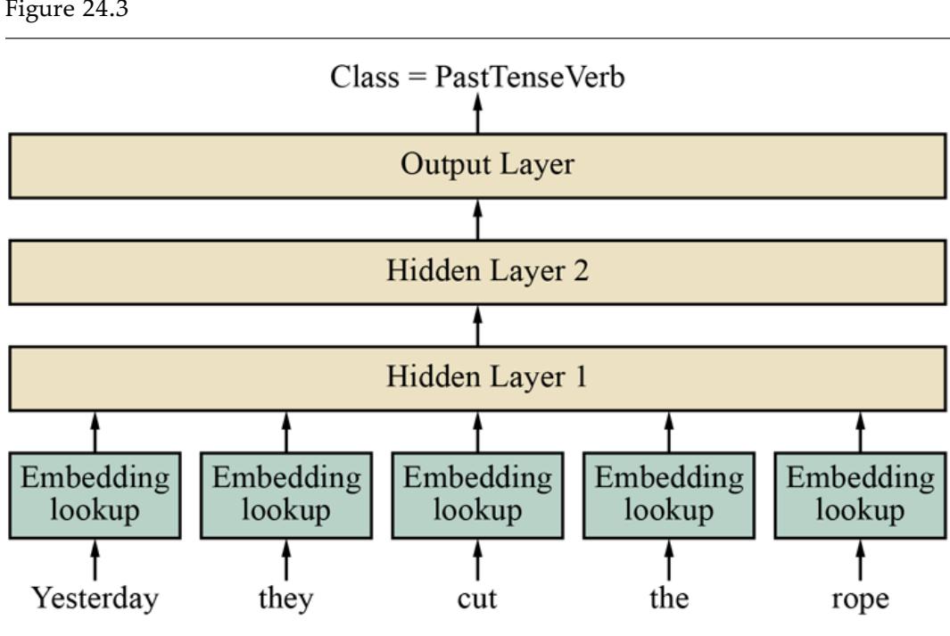
Feedforward part-of-speech tagging model. This model takes a 5-word window as input and predicts the tag of the word in the middle—here, cut. The model is able to account for word position because each of the 5 input embeddings is multiplied by a different part of the first hidden layer. The parameter values for the word embeddings and for the three layers are all learned simultaneously during training.

• 7. To encode a sequence of words into an input vector, simply look up the embedding for each word and concatenate the embedding vectors. The result is a real-valued input vector of length . Even though a given word will have the same embedding vector whether it occurs in the first position, the last, or somewhere in between, each embedding will be multiplied by a different part of the first hidden layer; therefore we are implicitly encoding the relative position of each word.
• 8. Train the weights and the other weight matrices , , and using gradient descent. If all goes well, the middle word, cut, will be labeled as a past-tense verb, based on the evidence in the window, which includes the temporal past word “yesterday,” the third-person subject pronoun “they” immediately before cut, and so on.

An alternative to word embeddings is a character-level model in which the input is a sequence of characters, each encoded as a one-hot vector. Such a model has to learn how characters come together to form words. The majority of work in NLP sticks with word-level rather than character-level encodings.

24.2 Recurrent Neural Networks for NLP

We now have a good representation for single words in isolation, but language consists of an ordered sequence of words in which the context of surrounding words is important. For simple tasks like part of speech tagging, a small, fixed-size window of perhaps five words usually provides enough context.

More complex tasks such as question answering or reference resolution may require dozens of words as context. For example, in the sentence “Eduardo told me that Miguel was very sick so I took him to the hospital,” knowing that him refers to Miguel and not Eduardo requires context that spans from the first to the last word of the 14-word sentence.

24.2.1 Language models with recurrent neural networks

We’ll start with the problem of creating a language model with sufficient context. Recall that a language model is a probability distribution over sequences of words. It allows us to predict the next word in a text given all the previous words, and is often used as a building block for more complex tasks.

Building a language model with either an -gram model (as in Section 23.1 ) or a feedforward network with a fixed window of words can run into difficulty due to the problem of context: either the required context will exceed the fixed window size or the model will have too many parameters, or both.

In addition, a feedforward network has the problem of asymmetry: whatever it learns about, say, the appearance of the word him as the 12th word of the sentence it will have to relearn for the appearance of him at other positions in the sentence, because the weights are different for each word position.

In Section 21.6 , we introduced the recurrent neural network or RNN, which is designed to process time-series data, one datum at a time. This suggests that RNNs might be useful for processing language, one word at a time. We repeat Figure 21.8 here as Figure 24.4 .

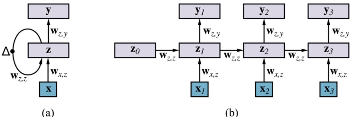
1. Schematic diagram of an RNN where the hidden layer has recurrent connections; the symbol indicates a delay. Each input is the word embedding vector of the next word in the sentence. Each output is the output for that time step. (b) The same network unrolled over three timesteps to create a feedforward network. Note that the weights are shared across all timesteps.

In an RNN language model each input word is encoded as a word embedding vector, . There is a hidden layer which gets passed as input from one time step to the next. We are interested in doing multiclass classification: the classes are the words of the vocabulary. Thus the output will be a softmax probability distribution over the possible values of the next word in the sentence.

The RNN architecture solves the problem of too many parameters. The number of parameters in the weight matrixes , , and stays constant, regardless of the number of words—it is . This is in contrast to feedforward networks, which have parameters, and -gram models, which have parameters, where is the size of the vocabulary.

The RNN architecture also solves the problem of asymmetry, because the weights are the same for every word position.

The RNN architecture can sometimes solve the limited context problem as well. In theory there is no limit to how far back in the input the model can look. Each update of the hidden layer has access to both the current input word and the previous hidden layer , which means that information about any word in the input can be kept in the hidden layer indefinitely, copied over (or modified as appropriate) from one time step to the next. Of course, there is a limited amount of storage in , so it can’t remember everything about all the previous words.

In practice RNN models perform well on a variety of tasks, but not on all tasks. It can be hard to predict whether they will be succesful for a given problem. One factor that contributes to success is that the training process encourages the network to allocate storage space in to the aspects of the input that will actually prove to be useful.

To train an RNN language model, we use the training process described in Section 21.6.1 . The inputs, , are the words in a training corpus of text, and the observed outputs are the same words offset by 1. That is, for the training text “hello world,” the first input is the word embedding for “hello” and the first output is the word embedding for “world.” We are training the model to predict the next word, and expecting that in order to do so it will use the hidden layer to represent useful information. As explained in Section 21.6.1 we compute the difference between the observed output and the actual output computed by the network, and back-propagate through time, taking care to keep the weights the same for all time steps.

Once the model has been trained, we can use it to generate random text. We give the model an initial input word , from which it will produce an output which is a softmax probability distribution over words. We sample a single word from the distribution, record the word as the output for time , and feed it back in as the next input word . We repeat for as long as desired. In sampling from we have a choice: we could always take the most likely word; we could sample according to the probability of each word; or we could oversample the less-likely words, in order to inject more variety into the generated output. The sampling weight is a hyperparameter of the model.

Here is an example of random text generated by an RNN model trained on Shakespeare’s works (Karpathy, 2015):

Marry, and will, my lord, to weep in such a one were prettiest; Yet now I was adopted heir Of the world’s lamentable day, To watch the next way with his father with his face?

24.2.2 Classification with recurrent neural networks

It is also possible to use RNNs for other language tasks, such as part of speech tagging or coreference resolution. In both cases the input and hidden layers will be the same, but for a POS tagger the output will be a softmax distribution over POS tags, and for coreference resolution it will be a softmax distribution over the posible antecedents. For example, when the network gets to the input him in “Eduardo told me that Miguel was very sick so I took him to the hospital” it should output a high probability for “Miguel.”

Training an RNN to do classification like this is done the same way as with the language model. The only difference is that the training data will require labels—part of speech tags or reference indications. That makes it much harder to collect the data than for the case of a language model, where unlabelled text is all we need.

In a language model we want to predict the th word given the previous words. But for classification, there is no reason we should limit ourselves to looking at only the previous words. It can be very helpful to look ahead in the sentence. In our coreference example, the referent him would be different if the sentence concluded “to see Miguel” rather than “to the hospital,” so looking ahead is crucial. We know from eye-tracking experiments that human readers do not go strictly left-to-right.

To capture the context on the right, we can use a bidirectional RNN, which concatenates a separate right-to-left model onto the left-to-right model. An example of using a bidirectional RNN for POS tagging is shown in Figure 24.5 .

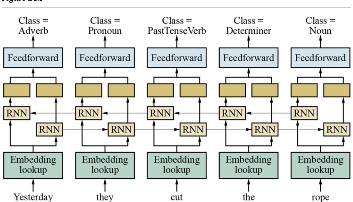
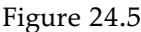
Bidirectional RNN

In the case of a multilayer RNN, will be the hidden vector of the last layer. For a bidirectional RNN, is usually taken to be the concatenation of vectors from the left-toright and right-to-left models.

RNNs can also be used for sentence-level (or document-level) classification tasks, in which a single output comes at the end, rather than having a stream of outputs, one per time step. For example in sentiment analysis the goal is to classify a text as having either Positive or Negative sentiment. For example, “This movie was poorly written and poorly acted” should be classified as Negative. (Some sentiment analysis schemes use more than two categories, or use a numeric scalar value.)

Using RNNs for a sentence-level task is a bit more complex, since we need to obtain an aggregate whole-sentence representation, from the per-word outputs of the RNN. The simplest way to do this is to use the RNN hidden state corresponding to the last word of the input, since the RNN will have read the entire sentence at that timestep. However, this can implicitly bias the model towards paying more attention to the end of the sentence. Another common technique is to pool all of the hidden vectors. For instance, average pooling computes the element-wise average over all of the hidden vectors:

\[\ddot{\mathbf{z}} = \frac{1}{s} \sum\_{t=1}^{s} \mathbf{z}\_t \dots\]

Average pooling

The pooled -dimensional vector can then be fed into one or more feedforward layers before being fed into the output layer.

24.2.3 LSTMs for NLP tasks

We said that RNNs sometimes solve the limited context problem. In theory, any information could be passed along from one hidden layer to the next for any number of time steps. But in practice the information can get lost or distorted, just as in playing the game of telephone, in which players stand in line and the first player whispers a message to the second, who repeats it to the third, and so on down the line. Usually, the message that comes out at the end is quite corrupted from the original message. This problem for RNNs is similar to the vanishing gradient problem we described on page 756, except that we are dealing now with layers over time rather than with deep layers.

In Section 21.6.2 we introduced the long short-term memory (LSTM) model. This is a kind of RNN with gating units that don’t suffer from the problem of imperfectly reproducing a message from one time step to the next. Rather, an LSTM can choose to remember some parts of the input, copying it over to the next timestep, and to forget other parts. Consider a language model handling a text such as

The athletes, who all won their local qualifiers and advanced to the finals in Tokyo, now …

At this point if we asked the model which next word was more probable, “compete” or “competes,” we would expect it to pick “compete” because it agrees with the subject “The athletes.” An LSTM can learn to create a latent feature for the subject person and number and copy that feature forward without alteration until it is needed to make a choice like this. A regular RNN (or an -gram model for that matter) often gets confused in long sentences with many intervening words between the subject and verb.

24.3 Sequence-to-Sequence Models

One of the most widely studied tasks in NLP is machine translation (MT), where the goal is to translate a sentence from a source language to a target language—for example, from Spanish to English. We train an MT model with a large corpus of source/target sentence pairs. The goal is to then accurately translate new sentences that are not in our training data.

Machine translation (MT)

Source language

Target language

Can we use RNNs to create an MT system? We can certainly encode the source sentence with an RNN. If there were a one-to-one correspondence between source words and target words, then we could treat MT as a simple tagging task—given the source word “perro” in Spanish, we tag it as the corresponding English word “dog.” But in fact, words are not oneto-one: in Spanish the three words “caballo de mar” corresponds to the single English word “seahorse,” and the two words “perro grande” translate to “big dog,” with the word order reversed. Word reordering can be even more extreme; in English the subject is usually at the start of a sentence, but in Fijian the subject is usually at the end. So how do we generate a sentence in the target language?

It seems like we should generate one word at a time, but keep track of the context so that we can remember parts of the source that haven’t been translated yet, and keep track of

what has been translated so that we don’t repeat ourselves. It also seems that for some sentences we have to process the entire source sentence before starting to generate the target. In other words, the generation of each target word is conditional on the entire source sentence and on all previously generated target words.

This gives text generation for MT a close connection to a standard RNN language model, as described in Section 24.2 . Certainly, if we had trained an RNN on English text, it would be more likely to generate “big dog” than “dog big.” However, we don’t want to generate just any random target language sentence; we want to generate a target language sentence that corresponds to the source language sentence. The simplest way to do that is to use two RNNs, one for the source and one for the target. We run the source RNN over the source sentence and then use the final hidden state from the source RNN as the initial hidden state for the target RNN. This way, each target word is implicitly conditioned on both the entire source sentence and the previous target words.

This neural network architecture is called a basic sequence-to-sequence model, an example of which is shown in Figure 24.6 . Sequence-to-sequence models are most commonly used for machine translation, but can also be used for a number of other tasks, like automatically generating a text caption from an image, or summarization: rewriting a long text into a shorter one that maintains the same meaning.

Basic sequence-to-sequence model. Each block represents one LSTM timestep. (For simplicity, the embedding and output layers are not shown.) On successive steps we feed the network the words of the source sentence “The man is tall,” followed by the tag to indicate that the network should start producing the target sentence. The final hidden state at the end of the source sentence is used as the hidden state for the start of the target sentence. After that, each target sentence word at time is used as input at time , until the network produces the tag to indicate that sentence generation is finished.

Sequence-to-sequence model

Basic sequence-to-sequence models were a significant breakthrough in NLP and MT specifically. According to Wu et al. (2016b) the approach led to a 60% error reduction over the previous MT methods. But these models suffer from three major shortcomings:

• NEARBY CONTEXT BIAS: whatever RNNs want to remember about the past, they have to fit into their hidden state. For example, let’s say an RNN is processing word (or timestep) 57 in a 70-word sequence. The hidden state will likely contain more information about the word at timestep 56 than the word at timestep 5, because each time the hidden vector is updated it has to replace some amount of existing information with new information. This behavior is part of the intentional design of the model, and often makes sense for NLP, since nearby context is typically more important. However, far-away context can be crucial as well, and can get lost in an RNN model; even LSTMs have difficulty with this task.
• FIXED CONTEXT SIZE LIMIT: In an RNN translation model the entire source sentence is compressed into a single fixed-dimensional hidden state vector. An LSTM used in a state-of-the-art NLP model typically has around 1024 dimensions, and if we have to represent, say, a 64-word sentence in 1024 dimensions, this only gives us 16 dimensions per word—not enough for complex sentences. Increasing the hidden state vector size can lead to slow training and overfitting.
• SLOWER SEQUENTIAL PROCESSING: As discussed in Section 21.3 , neural networks realize considerable efficiency gains by processing the training data in batches so as to take advantage of efficient hardware support for matrix arithmetic. RNNs, on the other hand, seem to be constrained to operate on the training data one word at a time.

24.3.1 Attention

What if the target RNN were conditioned on all of the hidden vectors from the source RNN, rather than just the last one? This would mitigate the shortcomings of nearby context bias and fixed context size limits, allowing the model to access any previous word equally well. One way to achieve this access is to concatenate all of the source RNN hidden vectors. However, this would cause a huge increase in the number of weights, with a concomitant

increase in computation time and potentially overfitting as well. Instead, we can take advantage of the fact that when the target RNN is generating the target one word at a time, it is likely that only a small part of the source is actually relevant to each target word.

Crucially, the target RNN must pay attention to different parts of the source for every word. Suppose a network is trained to translate English to Spanish. It is given the words “The front door is red” followed by an end of sentence marker, which means it is time to start outputting Spanish words. So ideally it should first pay attention to “The” and generate “La,” then pay attention to “door” and output “puerta,” and so on.

We can formalize this concept with a neural network component called attention, which can be used to create a “context-based summarization” of the source sentence into a fixeddimensional representation. The context vector contains the most relevant information for generating the next target word, and will be used as an additional input to the target RNN. A sequence-to-sequence model that uses attention is called an attentional sequence-tosequence model. If the standard target RNN is written as:

Attention

Attentional sequence-to-sequence model

the target RNN for attentional sequence-to-sequence models can be written as:

\[\mathbf{h}\_{i} = RNN(\mathbf{h}\_{i-1}, [\mathbf{x}\_{i}; \mathbf{c}\_{i}])\]

where is the concatenation of the input and context vectors, , defined as:

\[\begin{aligned} r\_{ij} &= \mathbf{h}\_{i-1} \cdot \mathbf{s}\_j\\ a\_{ij} &= e^{r\_{ij}} / \left(\sum\_k e^{r\_{ik}}\right),\\ \mathbf{c}\_i &= \sum\_j a\_{ij} \cdot \mathbf{s}\_j \end{aligned}\]

where is the target RNN vector that is going to be used for predicting the word at timestep , and is the output of the source RNN vector for the source word (or timestep) . Both and are -dimensional vectors, where is the hidden size. The value of is therefore the raw “attention score” between the current target state and the source word . These scores are then normalized into a probability using a softmax over all source words. Finally, these probabilities are used to generate a weighted average of the source RNN vectors, (another -dimensional vector).

An example of an attentional sequence-to-sequence model is given in Figure 24.7(a) . There are a few important details to understand. First, the attention component itself has no learned weights and supports variable-length sequences on both the source and target side. Second, like most of the other neural network modeling techniques we’ve learned about, attention is entirely latent. The programmer does not dictate what information gets used when; the model learns what to use. Attention can also be combined with multilayer RNNs. Typically attention is applied at each layer in that case.

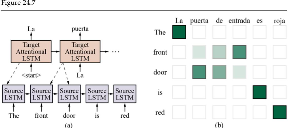
1. Attentional sequence-to-sequence model for English-to-Spanish translation. The dashed lines represent attention. (b) Example of attention probability matrix for a bilingual sentence pair, with darker boxes representing higher values of . The attention probabilities sum to one over each column.

The probabilistic softmax formulation for attention serves three purposes. First, it makes attention differentiable, which is necessary for it to be used with back-propagation. Even though attention itself has no learned weights, the gradients still flow back through attention to the source and target RNNs. Second, the probabilistic formulation allows the model to capture certain types of long-distance contextualization that may have not been captured by the source RNN, since attention can consider the entire source sequence at once, and learn to keep what is important and ignore the rest. Third, probabilistic attention allows the network to represent uncertainty—if the network does not know exactly what source word to translate next, it can distribute the attention probabilities over several options, and then actually choose the word using the target RNN.

Unlike most components of neural networks, attention probabilities are often interpretable by humans and intuitively meaningful. For example, in the case of machine translation, the attention probabilities often correspond to the word-to-word alignments that a human would generate. This is shown in Figure 24.7(b) .

Sequence-to-sequence models are a natural for machine translation, but almost any natural language task can be encoded as a sequence-to-sequence problem. For example, a questionanswering system can be trained on input consisting of a question followed by a delimiter followed by the answer.

24.3.2 Decoding

At training time, a sequence-to-sequence model attempts to maximize the probability of each word in the target training sentence, conditioned on the source and all of the previous target words. Once training is complete, we are given a source sentence, and our goal is to generate the corresponding target sentence. As shown in Figure 24.7 , we can generate the target one word at a time, and then feed back in the word that we generated at the next timestep. This procedure is called decoding.

Decoding

Greedy decoding

The simplest form of decoding is to select the highest probability word at each timestep and then feed this word as input to the next timestep. This is called greedy decoding because after each target word is generated, the system has fully committed to the hypothesis that it has produced so far. The problem is that the goal of decoding is to maximize the probability of the entire target sequence, which greedy decoding may not achieve. For example, consider using a greedy decoder to translate into Spanish the English sentence we saw before, The front door is red.

The correct translation is “La puerta de entrada es roja”—literally “The door of entry is red.” Suppose the target RNN correctly generates the first word La for The. Next, a greedy decoder might propose entrada for front. But this is an error—Spanish word order should put the noun puerta before the modifier. Greedy decoding is fast—it only considers one choice at each timestep and can do so quickly—but the model has no mechanism to correct mistakes.

We could try to improve the attention mechanism so that it always attends to the right word and guesses correctly every time. But for many sentences it is infeasible to guess correctly all the words at the start of the sentence until you have seen what’s at the end.

A better approach is to search for an optimal decoding (or at least a good one) using one of the search algorithms from Chapter 3 . A common choice is a beam search (see Section 4.1.3 ). In the context of MT decoding, beam search typically keeps the top hypotheses at each stage, extending each by one word using the top choices of words, then chooses the best of the resulting new hypotheses. When all hypotheses in the beam generate the special token, the algorithm outputs the highest scoring hypothesis.

A visualization of beam search is given in Figure 24.8 . As deep learning models become more accurate, we can usually afford to use a smaller beam size. Current state-of-the-art neural MT models use a beam size of 4 to 8, whereas the older generation of statistical MT models would use a beam size of 100 or more.

Figure 24.8

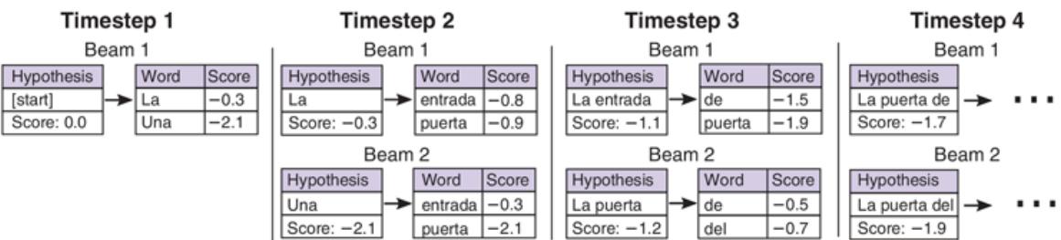
Beam search with beam size of . The score of each word is the log-probability generated by the target RNN softmax, and the score of each hypothesis is the sum of the word scores. At timestep 3, the highest scoring hypothesis La entrada can only generate low-probability continuations, so it “falls off the beam.”

24.4 The Transformer Architecture

The influential article “Attention is all you need” (Vaswani et al., 2018) introduced the transformer architecture, which uses a self-attention mechanism that can model longdistance context without a sequential dependency.

Transformer

Self-attention

24.4.1 Self-attention

Previously, in sequence-to-sequence models, attention was applied from the target RNN to the source RNN. Self-attention extends this mechanism so that each sequence of hidden states also attends to itself—the source to the source, and the target to the target. This allows the model to additionally capture long-distance (and nearby) context within each sequence.

Self-attention

The most straightforward way of applying self-attention is where the attention matrix is directly formed by the dot product of the input vectors. However, this is problematic. The dot product between a vector and itself will always be high, so each hidden state will be biased towards attending to itself. The transformer solves this by first projecting the input into three different representations using three different weight matrices:

The query vector is the one being attended from, like the target in the standard attention mechanism.

Query vector

The key vector is the one being attended to, like the source in the basic attention mechanism.

Key vector

The value vector is the context that is being generated.

Value vector

In the standard attention mechanism, the key and value networks are identical, but intuitively it makes sense for these to be separate representations. The encoding results of the th word, , can be calculated by applying an attention mechanism to the projected vectors:

\[r\_{ij} = (\mathbf{q}\_i \cdot \mathbf{k}\_j) / \sqrt{d}\]

\[a\_{ij} = e^{r\_{ij}} / (\sum\_k e^{r\_{kl}})\]

\[\mathbf{c}\_i = \sum\_j a\_{ij} \cdot \mathbf{v}\_j \,,\]

Multiheaded attention

where is the dimension of and . Note that and are indexes in the same sentence, since we are encoding the context using self-attention. In each transformer layer, selfattention uses the hidden vectors from the previous layer, which initially is the embedding layer.

There are several details worth mentioning here. First of all, the self-attention mechanism is asymmetric, as is different from . Second, the scale factor was added to improve numerical stability. Third, the encoding for all words in a sentence can be calculated simultaneously, as the above equations can be expressed using matrix operations that can be computed efficiently in parallel on modern specialized hardware.

The choice of which context to use is completely learned from training examples, not prespecified. The context-based summarization, , is a sum over all previous positions in the sentence. In theory, and information from the sentence could appear in , but in practice, sometimes important information gets lost, because it is essentially averaged out over the whole sentence. One way to address that is called multiheaded attention. We divide the sentence up into equal pieces and apply the attention model to each of the pieces. Each piece has its own set of weights. Then the results are concatenated together to form . By concatenating rather than summing, we make it easier for an important subpiece to stand out.

Multiheaded attention

24.4.2 From self-attention to transformer

Self-attention is only one component of the transformer model. Each transformer layer consists of several sub-layers. At each transformer layer, self-attention is applied first. The output of the attention module is fed through feedforward layers, where the same feedforward weight matrices are applied independently at each position. A nonlinear activation function, typically ReLU, is applied after the first feedforward layer. In order to address the potential vanishing gradient problem, two residual connections (are added into the transformer layer. A single-layer transformer in shown in Figure 24.9 . In practice, transformer models usually have six or more layers. As with the other models that we’ve learned about, the output of layer is used as the input to layer .

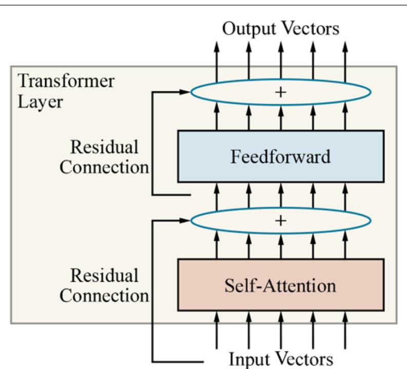
A single-layer transformer consists of self-attention, a feedforward network, and residual connections.

Positional embedding

Figure 24.9

The transformer architecture does not explicitly capture the order of words in the sequence, since context is modeled only through self-attention, which is agnostic to word order. To capture the ordering of the words, the transformer uses a technique called positional embedding. If our input sequence has a maximum length of , then we learn new embedding vectors—one for each word position. The input to the first transformer layer is the sum of the word embedding at position plus the positional embedding corresponding to position .

Figure 24.10 illustrates the transformer architecture for POS tagging, applied to the same sentence used in Figure 24.3 . At the bottom, the word embedding and the positional embeddings are summed to form the input for a three-layer transformer. The transformer produces one vector per word, as in RNN-based POS tagging. Each vector is fed into a final output layer and softmax layer to produce a probability distribution over the tags.

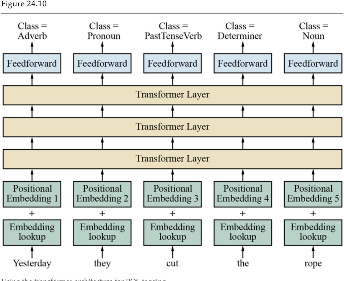
Using the transformer architecture for POS tagging.

In this section, we have actually only told half the transformer story: the model we described here is called the transformer encoder. It is useful for text classification tasks. The full transformer architecture was originally designed as a sequence-to-sequence model for machine translation. Therefore, in addition to the encoder, it also includes a transformer decoder. The encoder and decoder are nearly identical, except that the decoder uses a version of self-attention where each word can only attend to the words before it, since text is generated left-to-right. The decoder also has a second attention module in each transformer layer that attends to the output of the transformer encoder.

Transformer encoder

Transformer decoder

24.5 Pretraining and Transfer Learning

Getting enough data to build a robust model can be a challenge. In computer vision (see Chapter 25 ), that challenge was addressed by assembling large collections of images (such as ImageNet) and hand-labeling them.

For natural language, it is more common to work with text that is unlabeled. The difference is in part due to the difficulty of labeling: an unskilled worker can easily label an image as “cat” or “sunset,” but it requires extensive training to annotate a sentence with part-ofspeech tags or parse trees. The difference is also due to the abundance of text: the Internet adds over 100 billion words of text each day, including digitized books, curated resources such as Wikipedia, and uncurated social media posts.

Projects such as Common Crawl provide easy access to this data. Any running text can be used to build -gram or word embedding models, and some text comes with structure that can be helpful for a variety of tasks—for example, there are many FAQ sites with questionanswer pairs that can be used to train a question-answering system. Similarly, many Web sites publish side-by-side translations of texts, which can be used to train machine translation systems. Some text even comes with labels of a sort, such as review sites where users annotate their text reviews with a 5-star rating system.

We would prefer not to have to go to the trouble of creating a new data set every time we want a new NLP model. In this section, we introduce the idea of pretraining: a form of transfer learning (see Section 21.7.2 ) in which we use a large amount of shared generaldomain language data to train an initial version of an NLP model. From there, we can use a smaller amount of domain-specific data (perhaps including some labeled data) to refine the model. The refined model can learn the vocabulary, idioms, syntactic structures, and other linguistic phenomena that are specific to the new domain.

Pretraining

24.5.1 Pretrained word embeddings

In Section 24.1 , we briefly introduced word embeddings. We saw that how similar words like banana and apple end up with similar vectors, and we saw that we can solve analogy problems with vector subtraction. This indicates that the word embeddings are capturing substantial information about the words.

In this section we will dive into the details of how word embeddings are created using an entirely unsupervised process over a large corpus of text. That is in contrast to the embeddings from Section 24.1 , which were built during the process of supervised part of speech tagging, and thus required POS tags that come from expensive hand annotation.

We will concentrate on one specific model for word embeddings, the GloVe (Global Vectors) model. The model starts by gathering counts of how many times each word appears within a window of another word, similar to the skip-gram model. First choose window size (perhaps 5 words) and let be the number of times that words and cooccur within a window, and let be the number of times word co-occurs with any other word. Let be the probability that word appears in the context of word . As before, let be the word embedding for word .

Part of the intuition of the GloVe model is that the relationship between two words can best be captured by comparing them both to other words. Consider the words ice and steam. Now consider the ratio of their probabilities of co-occurrence with another word, , that is:

When is the word solid the ratio will be high (meaning solid applies more to ice) and when is the word gas it will be low (meaning gas applies more to steam). And when is a noncontent word like the, a word like water that is equally relevant to both, or an equally irrelevant word like fashion, the ratio will be close to 1.

The GloVe model starts with this intuition and goes through some mathematical reasoning (Pennington et al., 2014) that converts ratios of probabilities into vector differences and dot products, eventually arriving at the constraint

\[\mathbf{E}\_i \cdot \mathbf{E}\_k' = \log \left( P\_{ij} \right) \, .\]

In other words, the dot product of two word vectors is equal to the log probability of their co-occurrence. That makes intuitive sense: two nearly-orthogonal vectors have a dot product close to 0, and two nearly-identical normalized vectors have a dot product close to 1. There is a technical complication wherein the GloVe model creates two word embedding vectors for each word, and ; computing the two and then adding them together at the end helps limit overfitting.

Training a model like GloVe is typically much less expensive than training a standard neural network: a new model can be trained from billions of words of text in a few hours using a standard desktop CPU.

It is possible to train word embeddings on a specific domain, and recover knowledge in that domain. For example, Tshitoyan et al. (2019) used 3.3 million scientific abstracts on the subject of material science to train a word embedding model. They found that, just as we saw that a generic word embedding model can answer “Athens is to Greece as Oslo is to what?” with “Norway,” their material science model can answer “NiFe is to ferromagnetic as IrMn is to what?” with “antiferromagnetic.”

Their model does not rely solely on co-occurrence of words; it seems to be capturing more complex scientific knowledge. When asked what chemical compounds can be classified as “thermoelectric” or “topological insulator,” their model is able to answer correctly. For example, never appears near “thermoelectric” in the corpus, but it does appear near “chalcogenide,” “band gap,” and “optoelectric,” which are all clues enabling it to be classified as similar to “thermoelectric.” Furthermore, when trained only on abstracts up to the year 2008 and asked to pick compounds that are “thermoelectric” but have not yet appeared in abstracts, three of the model’s top five picks were discovered to be thermoelectric in papers published between 2009 and 2019.

24.5.2 Pretrained contextual representations

Word embeddings are better representations than atomic word tokens, but there is an important issue with polysemous words. For example, the word rose can refer to a flower or the past tense of rise. Thus, we expect to find at least two entirely distinct clusters of word contexts for rose: one similar to flower names such as dahlia, and one similar to upsurge. No single embedding vector can capture both of these simultaneously. Rose is a clear example of a word with (at least) two distinct meanings, but other words have subtle shades of

meaning that depend on context, such as the word need in you need to see this movie versus humans need oxygen to survive. And some idiomatic phrases like break the bank are better analyzed as a whole rather than as component words.

Therefore, instead of just learning a word-to-embedding table, we want to train a model to generate contextual representations of each word in a sentence. A contextual representation maps both a word and the surrounding context of words into a word embedding vector. In other words, if we feed this model the word rose and the context the gardener planted a rose bush, it should produce a contextual embedding that is similar (but not necessarily identical) to the representation we get with the context the cabbage rose had an unusual fragrance, and very different from the representation of rose in the context the river rose five feet.

Contextual representations

Figure 24.11 shows a recurrent network that creates contextual word embeddings—the boxes that are unlabeled in the figure. We assume we have already built a collection of noncontextual word embeddings. We feed in one word at a time, and ask the model to predict the next word. So for example in the figure at the point where we have reached the word “car,” the the RNN node at that time step will receive two inputs: the noncontextual word embedding for “car” and the context, which encodes information from the previous words “The red.” The RNN node will then output a contextual representation for “car.” The network as a whole then outputs a prediction for the next word, “is.” We then update the network’s weights to minimize the error between the prediction and the actual next word.

Figure 24.11

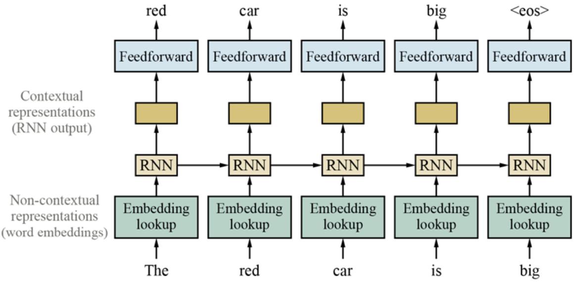
Training contextual representations using a left-to-right language model.

This model is similar to the one for POS tagging in Figure 24.5 , with two important differences. First, this model is unidirectional (left-to-right), whereas the POS model is bidirectional. Second, instead of predicting the POS tags for the current word, this model predicts the next word using the prior context. Once the model is built, we can use it to retrieve representations for words and pass them on to some other task; we need not continue to predict the next word. Note that computing a contextual representations always requires two inputs, the current word and the context.

24.5.3 Masked language models

A weakness of standard language models such as -gram models is that the contextualization of each word is based only on the previous words of the sentence. Predictions are made from left to right. But sometimes context from later in a sentence—for example, feet in the phrase rose five feet—helps to clarify earlier words.

One straightforward workaround is to train a separate right-to-left language model that contextualizes each word based on subsequent words in the sentence, and then concatenate the left-to-right and right-to-left representations. However, such a model fails to combine evidence from both directions.

Instead, we can use a masked language model (MLM). MLMs are trained by masking (hiding) individual words in the input and asking the model to predict the masked words. For this task, one can use a deep bidirectional RNN or transformer on top of the masked sentence. For example, given the input sentence “The river__rose five feet” we can mask the middle word to get “The river five feet” and ask the model to fill in the blank.

Masked language model (MLM)

The final hidden vectors that correspond to the masked tokens are then used to predict the words that were masked—in this example, rose. During training a single sentence can be used multiple times with different words masked out. The beauty of this approach is that it requires no labeled data; the sentence provides its own label for the masked word. If this model is trained on a large corpus of text, it generates pretrained representations that perform well across a wide variety of NLP tasks (machine translation, question answering, summarization, grammaticality judgments, and others).

24.6 State of the art

Deep learning and transfer learning have markedly advanced the state of the art for NLP—so much so that one commentator in 2018 declared that “NLP’s ImageNet moment has arrived” (Ruder, 2018). The implication is that just as a turning point occurred in 2012 for computer vision when deep learning systems produced surprising good results in the ImageNet competition, a turning point occurred in 2018 for NLP. The principal impetus for this turning point was the finding that transfer learning works well for natural language problems: a general language model can be downloaded and fine-tuned for a specific task.

It started with simple word embeddings from systems such WORD2VEC in 2013 and GloVe in 2014. Researchers can download such a model or train their own relatively quickly without access to supercomputers. Pretrained contextual representations, on the other hand, are orders of magnitude more expensive to train.

These models became feasible only after hardware advances (GPUs and TPUs) became widespread, and in this case researchers were grateful to be able to download models rather than having to spend the resources to train their own. The transformer model allowed for efficient training of much larger and deeper neural networks than was previously possible (this time due to software advances, not hardware). Since 2018, new NLP projects typically start with a pretrained transformer model.

Although these transformer models were trained to predict the next word in a text, they do a surprisingly good job at other language tasks. A ROBERTA model with some fine-tuning achieves state-of-the-art results in question answering and reading comprehension tests (Liu et al., 2019b). GPT-2, a transformer-like language model with 1.5 billion parameters trained on 40GB of Internet text, achieves good results on such diverse tasks as translation between French and English, finding referents of long-distance dependencies, and generalknowledge question answering, all without fine-tuning for the particular task. As Figure 24.14 illustrates, GPT-2 can generate fairly convincing text given just a few words as a prompt.

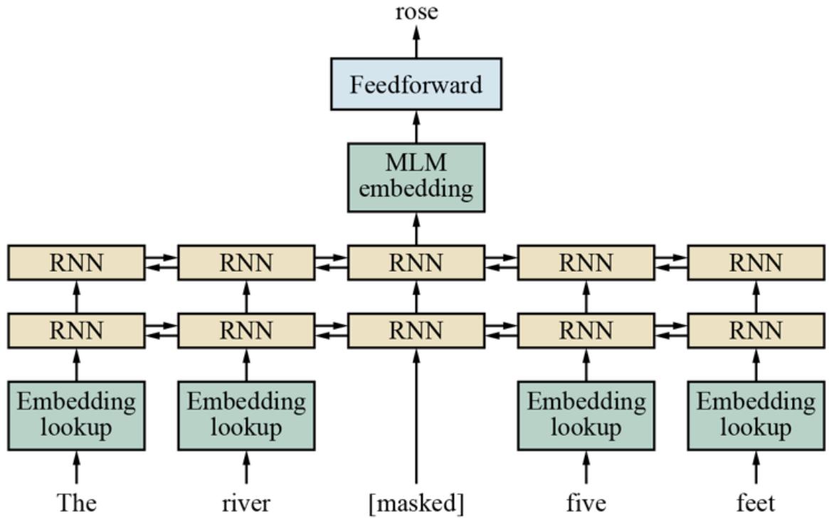
Masked language modeling: pretrain a bidirectional model—for example, a multilayer RNN—by masking input words and predicting only those masked words.

Figure 24.13

Questions from an 8th grade science exam that the ARISTO system can answer correctly using an ensemble of methods, with the most influential being a ROBERTA language model. Answering these questions requires knowledge about natural language, the structure of multiple-choice tests, commonsense, and science.

Figure 24.14

Example completion texts generated by the GPT-2 language model, given the prompts in bold. Most of the texts are quite fluent English, at least locally. The final example demonstrates that sometimes the model just breaks down.

As an example state-of-the-art NLP system, ARISTO (Clark et al., 2019) achieved a score of 91.6% on an 8th grade multiple-choice science exam (see Figure 24.13 ). ARISTO consists of an ensemble of solvers: some use information retrieval (similar to a web search engine), some do textual entailment and qualitative reasoning, and some use large transformer language models. It turns out that ROBERTA, by itself, scores 88.2% on the test. ARISTO also scores 83% on the more advanced 12th grade exam. (A score of 65% is considered “meeting the standards” and 85% is “meeting the standards with distinction”.)

There are limitations of ARISTO. It deals only with multiple-choice questions, not essay questions, and it can neither read nor generate diagrams. 1

1 It has been pointed out that in some multiple-choice exams, it is possible to get a good score even without looking at the questions, because there are tell-tale signs in the incorrect answers (Gururangan et al., 2018). That seems to be true for visual question answering as well (Chao et al., 2018).

T5 (the Text-to-Text Transfer Transformer) is designed to produce textual responses to various kinds of textual input. It includes a standard encoder–decoder transformer model, pretrained on 35 billion words from the 750 GB Colossal Clean Crawled Corpus (C4). This unlabeled training is designed to give the model generalizable linguistic knowledge that will be useful for multiple specific tasks. T5 is then trained for each task with input consisting of the task name, followed by a colon and some content. For example, when given “translate English to German: That is good,” it produces as output “Das ist gut.” For some tasks, the input is marked up; for example in the Winograd Schema Challenge, the input highlights a pronoun with an ambiguous referent. Given the input “referent: The city councilmen refused the demonstrators a permit because they feared violence,” the correct response is “The city councilmen” (not “the demonstrators”).

Much work remains to be done to improve NLP systems. One issue is that transformer models rely on only a narrow context, limited to a few hundred words. Some experimental approaches are trying to extend that context; the Reformer system (Kitaev et al., 2020) can handle context of up to a million words.

Recent results have shown that using more training data results in better models—for example, ROBERTA achieved state-of-the-art results after training on 2.2 trillion words. If using more textual data is better, what would happen if we included other types of data: structured databases, numerical data, images, and video? We would need a breakthrough in hardware processing speeds to train on a large corpus of video, and we may need several breakthroughs in AI as well.

The curious reader may wonder why we learned about grammars, parsing, and semantic interpretation in the previous chapter, only to discard those notions in favor of purely datadriven models in this chapter? At present, the answer is simply that the data-driven models are easier to develop and maintain, and score better on standard benchmarks, compared to the hand-built systems that can be constructed using a reasonable amount of human effort

with the approaches described in Chapter 23 . It may be that transformer models and their relatives are learning latent representations that capture the same basic ideas as grammars and semantic information, or it may be that something entirely different is happening within these enormous models; we simply don’t know. We do know that a system that is trained with textual data is easier to maintain and to adapt to new domains and new natural languages than a system that relies on hand-crafted features.

It may also be the case that future breakthroughs in explicit grammatical and semantic modeling will cause the pendulum to swing back. Perhaps more likely is the emergence of hybrid approaches that combine the best concepts from both chapters. For example, Kitaev and Klein (2018) used an attention mechanism to improve a traditional constituency parser, achieving the best result ever recorded on the Penn Treebank test set. Similarly, Ringgaard et al. (2017) demonstrate how a dependency parser can be improved with word embeddings and a recurrent neural network. Their system, SLING, parses directly into a semantic frame representation, mitigating the problem of errors building up in a traditional pipeline system.

There is certainly room for improvement: not only do NLP systems still lag human performance on many tasks, but they do so after processing thousands of times more text than any human could read in a lifetime. This suggests that there is plenty of scope for new insights from linguists, psychologists, and NLP researchers.

Summary

The key points of this chapter are as follows:

• Continuous representations of words with word embeddings are more robust than discrete atomic representations, and can be pretrained using unlabeled text data.
• Recurrent neural networks can effectively model local and long-distance context by retaining relevant information in their hidden-state vectors.
• Sequence-to-sequence models can be used for machine translation and text generation problems.
• Transformer models use self-attention and can model long-distance context as well as local context. They can make effective use of hardware matrix multiplication.
• Transfer learning that includes pretrained contextual word embeddings allows models to be developed from very large unlabeled corpora and applied to a range of tasks. Models that are pretrained to predict missing words can handle other tasks such as question answering and textual entailment, after fine-tuning for the target domain.

Bibliographical and Historical Notes

The distribution of words and phrases in natural language follow Zipf’s Law (Zipf, 1935, 1949): the frequency of the th most popular word is roughly inversely proportional to . That means we have a data sparsity problem: even with billions of words of training data, we are constantly running into novel words and phrases that were not seen before.

Generalization to novel words and phrases is aided by representations that capture the basic insight that words with similar meanings appear in similar contexts. Deerwester et al. (1990) projected words into low-dimensional vectors by decomposing the co-occurrence matrix formed by words and the documents the words appear in. Another possibility is to treat the surrounding words—say, a 5-word window—as context. Brown et al. (1992) grouped words into hierarchical clusters according to the bigram context of words; this has proven to be effective for tasks such as named entity recognition (Turian et al., 2010). The WORD2VEC system (Mikolov et al., 2013) was the first significant demonstration of the advantages of word embeddings obtained from training neural networks. The GloVe word embedding vectors (Pennington et al., 2014) were obtained by operating directly on a word cooccurrence matrix obtained from billions of words of text. Levy and Goldberg (2014) explain why and how these word embeddings are able to capture linguistic regularities.

Bengio et al. (2003) pioneered the use of neural networks for language models, proposing to combine “(1) a distributed representation for each word along with (2) the probability function for word sequences, expressed in terms of these representations.” Mikolov et al. (2010) demonstrated the use of RNNs for modeling local context in language models. Jozefowicz et al., (2016) showed how an RNN trained on a billion words can outperform carefully hand-crafted -gram models. Contextual representations for words were emphasized by Peters et al. (2018), who called them ELMO (Embeddings from Language Models) representations.

Note that some authors compare language models by measuring their perplexity. The perplexity of a probability distribution is , where is the entropy of the distribution (see Section 19.3.3 ). A language model with lower perplexity is, all other things being equal, a better model. But in practice, all other things are rarely equal. Therefore it is more informative to measure performance on a real task rather than relying on perplexity.

Perplexity

Howard and Ruder (2018) describe the ULMFIT (Universal Language Model Fine-tuning) framework, which makes it easier to fine-tune a pretrained language model without requiring a vast corpus of target-domain documents. Ruder et al. (2019) give a tutorial on transfer learning for NLP.

Mikolov et al. (2010) introduced the idea of using RNNs for NLP, and Sutskever et al. (2015) introduced the idea of sequence to sequence learning with deep networks. Zhu et al. (2017) and (Liu et al. 2018b) showed that an unsupervised approach works, and makes data collection much easier. It was soon found that these kinds of models could perform surprisingly well at a variety of tasks, for example, image captioning (Karpathy and Fei-Fei, 2015; Vinyals et al., 2017b).

Devlin et al. (2018) showed that transformer models pretrained with the masked language modeling objective can be directly used for multiple tasks. The model was called BERT (Bidirectional Encoder Representations from Transformers). Pretrained BERT models can be fine-tuned for particular domains and particular tasks, including question answering, named entity recognition, text classification, sentiment analysis, and natural language inference.

The XLNET system (Yang et al., 2019) improves on BERT by eliminating a discrepancy between the pretraining and fine-tuning. The ERNIE 2.0 framework (Sun et al., 2019) extracts more from the training data by considering sentence order and the presence of named entities, rather than just co-occurrence of words, and was shown to outperform BERT and XLNET. In response, researchers revisited and improved on BERT: the ROBERTA system (Liu et al., 2019b) used more data and different hyperparameters and training procedures, and found that it could match XLNET. The Reformer system (Kitaev et al., 2020) extends the range of the context that can be considered all the way up to a million words. Meanwhile, ALBERT (A Lite BERT) went in the other direction, reducing the number of parameters from 108 million to 12 million (so as to fit on mobile devices) while maintaining high accuracy.

The XLM system (Lample and Conneau, 2019) is a transformer model with training data from multiple languages. This is useful for machine translation, but also provides more

robust representations for monolingual tasks. Two other important systems, GPT-2 (Radford et al., 2019) and T5 (Raffel et al., 2019), were described in the chapter. The later paper also introduced the 35 billion word Colossal Clean Crawled Corpus (C4).

Various promising improvements on pretraining algorithms have been proposed (Yang et al., 2019; Liu et al., 2019b). Pretrained contextual models are described by Peters et al. (2018) and Dai and Le (2016).

The GLUE (General Language Understanding Evaluation) benchmark, a collection of tasks and tools for evaluating NLP systems, was introduced by Wang et al. (2018a). Tasks include question answering, sentiment analysis, textual entailment, translation, and parsing. Transformer models have so dominated the leaderboard (the human baseline is way down at ninth place) that a new version, SUPERGLUE (Wang et al., 2019), was introduced with tasks that are designed to be harder for computers, but still easy for humans.

At the end of 2019, T5 was the overall leader with a score of 89.3, just half a point below the human baseline of 89.8. On three of the ten tasks, T5 actually exceeds human performance: yes/no question answering (such as “Is France the same time zone as the UK?”) and two reading comprehension tasks involving answering questions after reading either a paragraph or a news article.

Machine translation is a major application of language models. In 1933, Petr Troyanskii received a patent for a “translating machine,” but there were no computers available to implement his ideas. In 1947, Warren Weaver, drawing on work in cryptography and information theory, wrote to Norbert Wiener: “When I look at an article in Russian, I say: ‘This is really written in English, but it has been coded in strange symbols. I will now proceed to decode.”’ The community proceeded to try to decode in this way, but they didn’t have sufficient data and computing resources to make the approach practical.

In the 1970s that began to change, and the SYSTRAN system (Toma, 1977) was the first commercially successful machine translation system. SYSTRAN relied on lexical and grammatical rules hand-crafted by linguists as well as on training data. In the 1980s, the community embraced purely statistical models based on frequency of words and phrases (Brown et al., 1988; Koehn, 2009). Once training sets reached billions or trillions of tokens (Brants et al., 2007), this yielded systems that produced comprehensible but not fluent

results (Och and Ney, 2004; Zollmann et al., 2008). Och and Ney (2002) show how discriminative training led to an advance in machine translation in the early 2000s.

Sutskever et al. (2015) first showed that it is possible to learn an end-to-end sequence-tosequence neural model for machine translation. Bahdanau et al. (2015) demonstrated the advantage of a model that jointly learns to align sentences in the source and target language and to translate between the languages. Vaswani et al. (2018) showed that neural machine translation systems can further be improved by replacing LSTMs with transformer architectures, which use the attention mechanism to capture context. These neural translation systems quickly overtook statistical phrase-based methods, and the transformer architecture soon spread to other NLP tasks.

Research on question answering was facilitated by the creation of SQUAD, the first largescale data set for training and testing question-answering systems (Rajpurkar et al., 2016). Since then, a number of deep learning models have been developed for this task (Seo et al., 2017; Keskar et al., 2019). The ARISTO system (Clark et al., 2019) uses deep learning in conjunction with an ensemble of other tactics. Since 2018, the majority of questionanswering models use pretrained language representations, leading to a noticeable improvement over earlier systems.

Natural language inference is the task of judging whether a hypothesis (dogs need to eat) is entailed by a premise (all animals need to eat). This task was popularized by the PASCAL Challenge (Dagan et al., 2005). Large-scale data sets are now available (Bowman et al., 2015; Williams et al., 2018). Systems based on pretrained models such as ELMO and BERT currently provide the best performance on language inference tasks.

The Conference on Computational Natural Language Learning (CoNLL) focuses on learning for NLP. All the conferences and journals mentioned in Chapter 23 now include papers on deep learning, which now has a dominant position in the field of NLP.

Chapter 25 Computer Vision

In which we connect the computer to the raw, unwashed world through the eyes of a camera.

Most animals have eyes, often at significant cost: eyes take up a lot of space; use energy; and are quite fragile. This cost is justified by the immense value that eyes provide. An agent that can see can predict the future—it can tell what it might bump into; it can tell whether to attack or to flee or to court; it can guess whether the ground ahead is swampy or firm; and it can tell how far away the fruit is. In this chapter, we describe how to recover information from the flood of data that comes from eyes or cameras.

25.1 Introduction

Vision is a perceptual channel that accepts a stimulus and reports some representation of the world. Most agents that use vision use passive sensing—they do not need to send out light to see. In contrast, active sensing involves sending out a signal such as radar or ultrasound, and sensing a reflection. Examples of agents that use active sensing include bats (ultrasound), dolphins (sound), abyssal fishes (light), and some robots (light, sound, radar). To understand a perceptual channel, one must study both the physical and statistical phenomena that occur in sensing and what the perceptual process should produce. We concentrate on vision in this chapter, but robots in the real world use a variety of sensors to perceive sound, touch, distance, temperature, global position, and acceleration.

A feature is a number obtained by applying simple computations to an image. Very useful information can be obtained directly from features. The wumpus agent had five sensors, each of which extracted a single bit of information. These bits, which are features, could be interpreted directly by the program. As another example, many flying animals compute a simple feature that gives a good estimate of time to contact with a nearby object; this feature can be passed directly to muscles that control steering or wings, allowing very fast changes of direction. This feature extraction approach emphasizes simple, direct computations applied to sensor responses.

Feature

The model-based approach to vision uses two kinds of models. An object model could be the kind of precise geometric model produced by computer aided design systems. It could also be a vague statement about general properties of objects, for example, the claim that all faces viewed in low resolution look approximately the same. A rendering model describes the physical, geometric, and statistical processes that produce the stimulus from the world. While rendering models are now sophisticated and exact, the stimulus is usually ambiguous. A white object under low light may look like a black object under intense light. A small,

nearby object may look the same as a large, distant object. Without additional evidence, we cannot tell if what we see is a toy Godzilla tearing up a toy building, or a real monster destroying a real building.

There are two main ways to manage these ambiguities. First, some interpretations are more likely than others. For example, we can be confident that the picture doesn’t show a real Godzilla destroying a real building, because there are no real Godzillas. Second, some ambiguities are insignificant. For example, distant scenery may be trees or may be a flat painted surface. For most applications, the difference is unimportant, because the objects are far away and so we will not bump into them or interact with them soon.

The two core problems of computer vision are reconstruction, where an agent builds a model of the world from an image or a set of images, and recognition, where an agent draws distinctions among the objects it encounters based on visual and other information. Both problems should be interpreted very broadly. Building a geometric model from images is obviously reconstruction (and solutions are very valuable), but sometimes we need to build a map of the different textures on a surface, and this is reconstruction, too. Attaching names to objects that appear in an image is clearly recognition. Sometimes we need to answer questions like: Is it asleep? Does it eat meat? Which end has teeth? Answering these questions is recognition, too.

Reconstruction

Recognition

The last thirty years of research have produced powerful tools and methods for addressing these core problems. Understanding these methods requires an understanding of the processes by which images are formed.

25.2 Image Formation

Imaging distorts the appearance of objects. A picture taken looking down a long straight set of railway tracks will suggest that the rails converge and meet. If you hold your hand in front of your eye, you can block out the moon, even though the moon is larger than your hand (this works with the sun too, but you could damage your eyes checking it). If you hold a book flat in front of your face and tilt it backward and forward, it will seem to shrink and grow in the image. This effect is known as foreshortening (Figure 25.1 ). Models of these effects are essential for building competent object recognition systems and also yield powerful cues for reconstructing geometry.

Figure 25.1

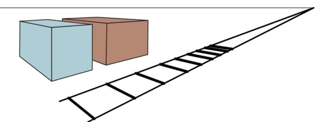
Geometry in the scene appears distorted in images. Parallel lines appear to meet, like the railway tracks in a desolate town. Buildings that have right angles in the real world scene have distorted angles in the image.

25.2.1 Images without lenses: The pinhole camera

Image sensors gather light scattered from objects in a scene and create a two-dimensional (2D) image. In the eye, these sensors consist of two types of cell: There are about 100 million rods, which are sensitive to light at a wide range of wavelengths, and 5 million cones. Cones, which are essential for color vision, are of three main types, each of which is sensitive to a different set of wavelengths. In cameras, the image is formed on an image plane. In film cameras the image plane is coated with silver halides. In digital cameras, the image plane is subdivided into a grid of a few million pixels.

Scene
Image
Pixels
Sensor

We refer to the whole image plane as a sensor, but each pixel is an individual tiny sensor usually a charge-coupled device (CCD) or complementary metal-oxide semiconductor (CMOS). Each photon arriving at the sensor produces an electrical effect, whose strength depends on the wavelength of the photon. The output of the sensor is the sum of all these effects in some time window, meaning that image sensors report a weighted average of the intensity of light arriving at the sensor. The average is over wavelength, direction from which photons can arrive, time, and the area of the sensor.

To see a focused image, we must ensure that all the photons arriving at a sensor come from approximately the same spot on the object in the world. The simplest way to form a focused image is to view stationary objects with a pinhole camera, which consists of a pinhole opening, , at the front of a box, and an image plane at the back of the box (Figure 25.2 ). The opening is called the aperture. If the pinhole is small enough, each tiny sensor in the image plane will see only photons that come from approximately the same spot on the object, and so the image is focused. We can form focused images of moving objects with a pinhole camera, too, as long as the object moves only a short distance in the sensors’ time window. Otherwise, the image of the moving object is defocused, an effect known as motion blur. One way to manipulate the time window is to open and close the pinhole.

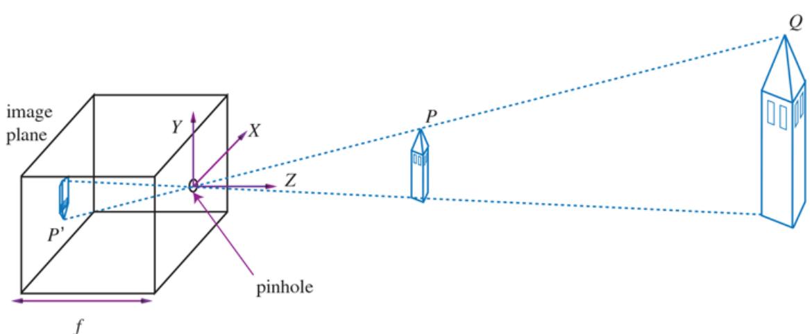
Each light sensitive element at the back of a pinhole camera receives light that passes through the pinhole from a small range of directions. If the pinhole is small enough, the result is a focused image behind the pinhole. The process of projection means that large, distant objects look the same as smaller, nearby objects—the point in the image plane could have come from a nearby toy tower at point or from a distant real tower at point .

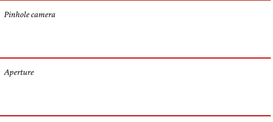
Motion blur

Pinhole cameras make it easy to understand the geometric model of camera behavior (which is more complicated—but similar—with most other imaging devices). We will use a three-dimensional (3D) coordinate system with the origin at , and will consider a point in the scene, with coordinates . gets projected to the point in the image plane with coordinates . If is the focal length—the distance from the pinhole to the image plane—then by similar triangles, we can derive the following equations:

\[\frac{-x}{f} = \frac{X}{Z}, \frac{-y}{f} = \frac{Y}{Z} \quad \Rightarrow \quad x = \frac{-fX}{Z}, \ y = \frac{-fY}{Z} \; .\]

Focal length

These equations define an image formation process known as perspective projection. Note that the in the denominator means that the farther away an object is, the smaller its image will be. Also, note that the minus signs mean that the image is inverted, both left–right and up–down, compared with the scene.

Perspective projection

Perspective imaging has a number of geometric effects. Distant objects look small. Parallel lines converge to a point on the horizon. (Think of railway tracks, Figure 25.1 .) A line in the scene in the direction and passing through the point can be described as the set of points , with varying between and . Different choices of yield different lines parallel to one another. The projection of a point from this line onto the image plane is given by

\[P\_{\lambda} = \left( f \frac{X\_0 + \lambda U}{Z\_0 + \lambda W}, f \frac{Y\_0 + \lambda V}{Z\_0 + \lambda W} \right).\]

As or , this becomes if . This means that two parallel lines leaving different points in space will converge in the image—for large , the image points are nearly the same, whatever the value of (again, think railway tracks, Figure 25.1 ). We call the vanishing point associated with the family of straight lines with direction . Lines with the same direction share the same vanishing point.

25.2.2 Lens systems

Pinhole cameras can focus light well, but because the pinhole is small, only a little light will get in, and the image will be dark. Over a short period of time, only a few photons will hit each point on the sensor, so the signal at each point will be dominated by random fluctuations; we say that a dark film image is grainy and a dark digital image is noisy; either way, the image is of low quality.

Enlarging the hole (the aperture) will make the image brighter by collecting more light from a wider range of directions. However, with a larger aperture the light that hits a particular point in the image plane will have come from multiple points in the real world scene, so the image will be defocused. We need some way to refocus the image.

Vertebrate eyes and modern cameras use a lens system—a single piece of transparent tissue in the eye and a system of multiple glass lens elements in a camera. In Figure 25.3 we see that light from the tip of the candle spreads out in all directions. A camera (or an eye) with a lens captures all the light that hits anywhere on the lens—a much larger area than a pinhole —and focuses all that light to a single point on the image plane. Light from other parts of the candle would similarly be gathered and focused to other points on the image plane. The result is a brighter, less noisy, focused image.

Figure 25.3

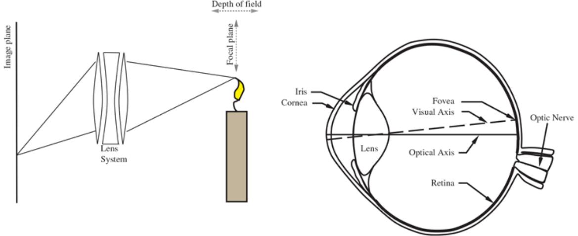
Lenses collect the light leaving a point in the scene (here, the tip of the candle flame) in a range of directions, and steer all the light to arrive at a single point on the image plane. Points in the scene near the focal plane—within the depth of field—will be focused properly. In cameras, elements of the lens system move to change the focal plane, whereas in the eye, the shape of the lens is changed by specialized muscles.

Lens

Lens systems do not focus all the light from everywhere in the real world; the lens design restricts them to focusing light only from points that lie within a range of depths from the lens. The center of this range—where focus is sharpest—is called the focal plane, and the range of depths for which focus remains sharp enough is called the depth of field. The larger the lens aperture (opening), the smaller the depth of field.

Focal plane

Depth of field

What if you want to focus on something at a different distance? To move the focal plane, the lens elements in a camera can move back and forth, and the lens in the eye can change shape—but with age the eye lens tends to harden, making it less able to adjust focal distances, and requiring many humans to augment their vision with external lens eyeglasses.

25.2.3 Scaled orthographic projection

The geometric effects of perspective imaging aren’t always pronounced. For example, windows on a building across the street look much smaller than ones right nearby, but two windows that are next to each other will have about the same size even though one is slightly farther away. We have the option to handle the windows with a simplified model called scaled orthographic projection, rather than perspective projection. If the depth of all points on an object fall within the range , with , then the perspective scaling factor can be approximated by a constant . The equations for projection from the scene coordinates to the image plane become and . Foreshortening still occurs in the scaled orthographic projection model, because it is caused by the object tilting away from the view.

Scaled orthographic projection

25.2.4 Light and shading

The brightness of a pixel in the image is a function of the brightness of the surface patch in the scene that projects to the pixel. For modern cameras, this function is linear for middling intensities of light, but has pronounced nonlinearities for darker and brighter illumination. We will use a linear model. Image brightness is a strong, if ambiguous, cue to both the shape and the identity of objects. The ambiguity occurs because there are three factors that contribute to the amount of light that comes from a point on an object to the image: the overall intensity of ambient light); whether the point is facing the light or is in shadow); and the amount of light reflected from the point.

Ambient light

Reflection

People are surprisingly good at disambiguating brightness—they usually can tell the difference between a black object in bright light and a white object in shadow, even if both have the same overall brightness. However, people sometimes get shading and markings mixed up—-a streak of dark makeup under a cheekbone will often look like a shading effect, making the face look thinner.

Most surfaces reflect light by a process of diffuse reflection. Diffuse reflection scatters light evenly across the directions leaving a surface, so the brightness of a diffuse surface doesn’t depend on the viewing direction. Most cloth has this property, as do most paints, rough wooden surfaces, most vegetation, and rough stone or concrete.

Diffuse reflection

Specular reflection causes incoming light to leave a surface in a lobe of directions that is determined by the direction the light arrived from. A mirror is one example. What you see depends on the direction in which you look at the mirror. In this case, the lobe of directions is very narrow, which is why you can resolve different objects in a mirror.

Specular reflection

For many surfaces, the lobe is broader. These surfaces display small bright patches, usually called specularities. As the surface or the light moves, the specularities move, too. Away from these patches, the surface behaves as if it is diffuse. Specularities are often seen on metal surfaces, painted surfaces, plastic surfaces, and wet surfaces. These are easy to identify, because they are small and bright (Figure 25.4 ). For almost all purposes, it is enough to model all surfaces as being diffuse with specularities.

Figure 25.4

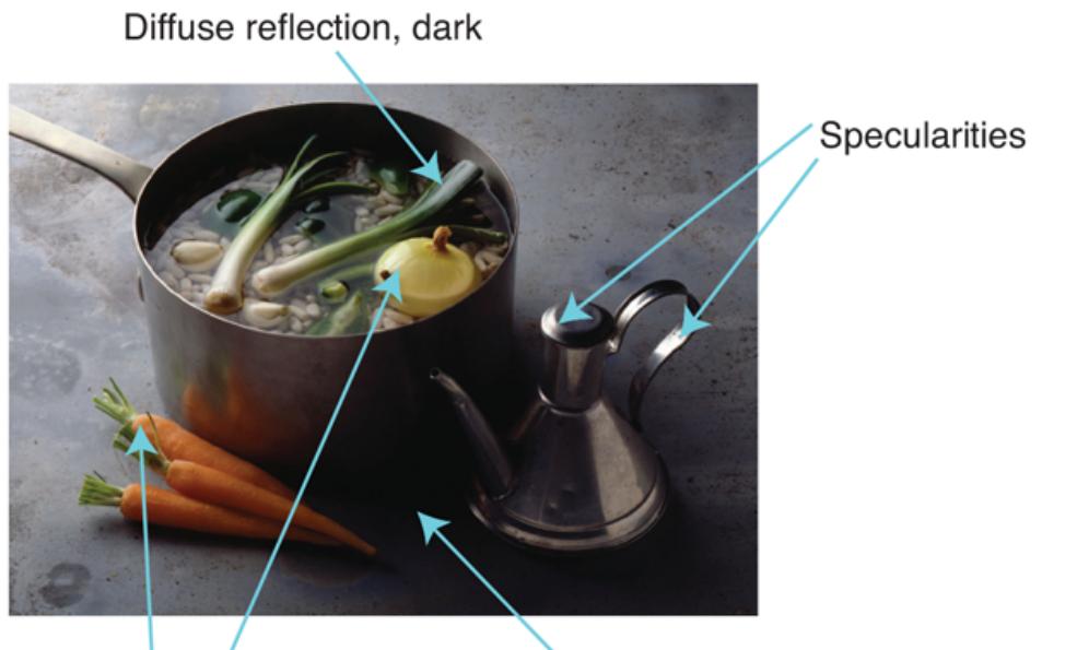
This photograph illustrates a variety of illumination effects. There are specularities on the stainless steel cruet. The onions and carrots are bright diffuse surfaces because they face the light direction. The shadows appear at surface points that cannot see the light source at all. Inside the pot are some dark diffuse surfaces where the light strikes at a tangential angle. (There are also some shadows inside the pot.)

Photo by Ryman Cabannes/Image Professionals GmbH/Alamy Stock Photo.

Specularities

The main source of illumination outside is the sun, whose rays all travel parallel to one another in a known direction because it is so far away. We model this behavior with a

distant point light source. This is the most important model of lighting, and is quite effective for indoor scenes as well as outdoor scenes. The amount of light collected by a surface patch in this model depends on the angle between the illumination direction and the normal (perpendicular) to the surfaces (Figure 25.5 ).

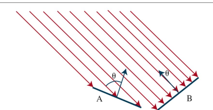
Two surface patches are illuminated by a distant point source, whose rays are shown as light arrows. Patch A is tilted away from the source ( is close to ) and collects less energy, because it cuts fewer light rays per unit surface area. Patch B, facing the source ( is close to ), collects more energy.

Distant point light source

Figure 25.5

A diffuse surface patch illuminated by this model will reflect some fraction of the light it collects, given by the diffuse albedo. For practical surfaces, this lies in the range 0.05-0.95. Lambert’s cosine law states the brightness of a diffuse patch is given by

\[I = \rho I\_0 \cos \theta,\]

Diffuse albedo

Lambert’s cosine law

Shadow

where is the intensity of the light source, is the angle between the light source direction and the surface normal, and is the diffuse albedo. This law predicts that bright image pixels come from surface patches that face the light directly and dark pixels come from patches that see the light only tangentially, so that the shading on a surface provides some shape information. If the surface cannot see the source, then it is in shadow. Shadows are very seldom a uniform black, because the shadowed surface usually receives some light from other sources. Outdoors, the most important source other than the sun is the sky, which is quite bright. Indoors, light reflected from other surfaces illuminates shadowed patches. These interreflections can have a significant effect on the brightness of other surfaces, too. These effects are sometimes modeled by adding a constant ambient illumination term to the predicted intensity.

Interreflections

Ambient illumination

25.2.5 Color

Fruit is a bribe that a tree offers to animals to carry its seeds around. Trees that can signal when this bribe is ready have an advantage, as do animals that can read these signals. As a result, most fruits start green, and turn red or yellow when ripe, and most fruit-eating animals can see these color changes. Generally, light arriving at the eye has different amounts of energy at different wavelengths, and is represented by a spectral energy density. Cameras and the human vision system respond to light at wavelengths ranging from about 380nm (violet) to about 750nm (red). In color imaging systems, there are different types of receptor that respond more or less strongly to different wavelengths. In humans, the sensation of color occurs when the vision system compares the responses of receptors near each other on the retina. Animal color vision systems typically have relatively few types of receptor, and so represent relatively little of the detail in the spectral energy density function (some animals have only one type of receptor; some have as many as six types). Human color vision is produced by three types of receptor. Most color camera systems use only three types of receptor, too, because the images are produced for humans, but some specialized systems can produce very detailed measurements of the spectral energy density.

Because most humans have three types of color-sensitive receptors, the principle of trichromacy applies. This idea, first proposed by Thomas Young in 1802, states that a human observer can match the visual appearance of any spectral energy density, however complex, by mixing appropriate amounts of just three primaries. Primaries are colored light sources, chosen so that no mixture of any two will match the third. A common choice is to have one red primary, one green, and one blue, abbreviated as RGB. Although a given colored object may have many component frequencies of light, we can match the color by mixing just the three primaries, and most people will agree on the proportions of the mixture. That means we can represent color images with just three numbers per pixel—the RGB values.

Principle of trichromacy

Primaries

RGB

For most computer vision applications, it is accurate enough to model a surface as having three different (RGB) diffuse albedos and to model light sources as having three (RGB) intensities. We then apply Lambert’s cosine law to each to get red, green, and blue pixel values. This model predicts, correctly, that the same surface will produce different colored image patches under different colored lights. In fact, human observers are quite good at ignoring the effects of different colored lights and appear to estimate the color the surface would have under white light, an effect known as color constancy.

Color constancy

25.3 Simple Image Features

Light reflects off objects in the scene to form an image consisting of, say, twelve million three-byte pixels. As with all sensors there will be noise in the image, and in any case there is a lot of data to deal with. The way to get started analyzing this data is to produce simplified representations that expose what’s important, but reduce detail. Much current practice learns these representations from data. But there are four properties of images and video that are particularly general: edges, texture, optical flow and segmentation into regions.

An edge occurs where there is a big difference in pixel intensity across part of an image. Building representations of edges involves local operations on an image—you need to compare a pixel value to some values nearby—and doesn’t require any knowledge about what is in the image. Thus, edge detection can come early in the pipeline of operations and we call it an “early” or “low-level” operation.

The other operations require handling a larger area of the image. For example, a texture description applies to a pool of pixels—to say “stripey,” you need to see some stripes. Optical flow represents where pixels move to from one image in a sequence to the next, and this can cover a larger area. Segmentation cuts an image into regions of pixels that naturally belong together, and doing so requires looking at the whole region. Operations like this are sometimes referred to as “mid-level” operations.

25.3.1 Edges

Edges are straight lines or curves in the image plane across which there is a “significant” change in image brightness. The goal of edge detection is to abstract away from the messy, multi-megabyte image and towards a more compact, abstract representation, as in Figure 25.6 . Effects in the scene very often result in large changes in image intensity, and so produce edges in the image. Depth discontinuities (labeled 1 in the figure) can cause edges because when you cross the discontinuity, the color typically changes. When the surface normal changes (labeled 2 in the figure), the image intensity often changes. When the surface reflectance changes (labeled 3), the image intensity often changes. Finally, a shadow (labeled 4) is a discontinuity in illumination that causes an edge in the image, even though

there is not an edge in the object. Edge detectors can’t disentangle the cause of the discontinuity, which is left to later processing.

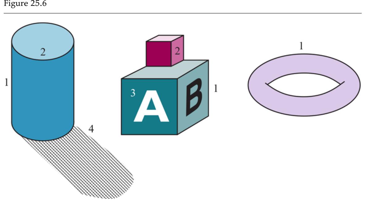
Different kinds of edges: (1) depth discontinuities; (2) surface orientation discontinuities; (3) reflectance discontinuities; (4) illumination discontinuities (shadows).

Edges

Finding edges requires care. Figure 25.7 (top) shows a one-dimensional crosssection of an image perpendicular to an edge, with an edge at .

Figure 25.7

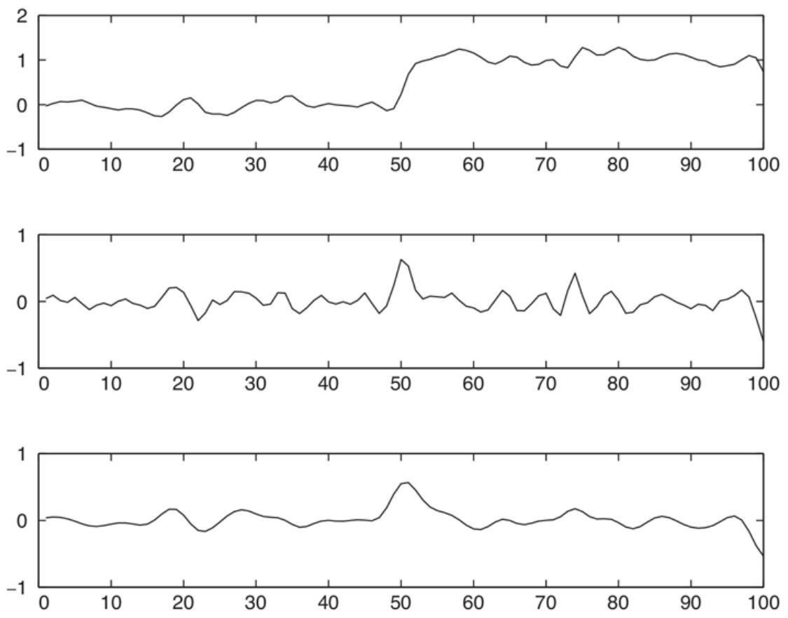
Top: Intensity profile along a one-dimensional section across a step edge. Middle: The derivative of intensity, . Large values of this function correspond to edges, but the function is noisy. Bottom: The derivative of a smoothed version of the intensity. The noisy candidate edge at has disappeared.

Noise

You might differentiate the image and look for places where the magnitude of the derivative is large. This almost works, but in Figure 25.7 (middle), we see that although there is a peak at , there are also subsidiary peaks at other locations (e.g., ) that could be mistaken for true edges. These arise because of the presence of “noise” in the image. Noise here means changes to the value of a pixel that don’t have to do with an edge. For example, there could be thermal noise in the camera; there could be scratches on the object surface that change the surface normal at the finest scale; there could be minor variations in the surface albedo; and so on. Each of these effects make the gradient look big, but don’t

mean that an edge is present. If we “smooth” the image first, the spurious peaks are diminished, as we see in Figure 25.7 (bottom).

Smoothing involves using surrounding pixels to suppress noise. We will predict the “true” value of our pixel as a weighted sum of nearby pixels, with more weight for the closest pixels. A natural choice of weights is a Gaussian filter. Recall that the zero-mean Gaussian function with standard deviation is

\[\begin{aligned} G\_{\sigma}(x) &= \frac{1}{\sqrt{2\pi}\sigma} e^{-x^2/2\sigma^2} & \text{in one dimension, or} \\ G\_{\sigma}(x,y) &= \frac{1}{2\pi\sigma^2} e^{-(x^2+y^2)/2\sigma^2} & \text{in two dimensions.} \end{aligned}\]

Gaussian filter

Applying a Gaussian filter means replacing the intensity with the sum, over all pixels, of , where is the distance from to . This kind of weighted sum is so common that there is a special name and notation for it. We say that the function is the convolution of two functions and (denoted as ) if we have

\[\begin{aligned} h(x) &= \sum\_{u = -\infty}^{+\infty} f(u)g(x - u) \quad \text{in one dimension, or} \\ h(x, y) &= \sum\_{u = -\infty}^{+\infty} \sum\_{v = -\infty}^{+\infty} f(u, v)g(x - u, y - v) \quad \text{in two dimensions.} \end{aligned}\]

Convolution

So the smoothing function is achieved by convolving the image with the Gaussian, . A of 1 pixel is enough to smooth over a small amount of noise, whereas 2 pixels will smooth a larger amount, but at the loss of some detail. Because the Gaussian’s influence fades

rapidly with distance, in practice we can replace the in the sums with something like .

We have a chance to make an optimization here: we can combine the smoothing and the edge finding into a single operation. It is a theorem that for any functions and , the derivative of the convolution, , is equal to the convolution with the derivative, . So rather than smoothing the image and then differentiating, we can just convolve the image with the derivative of the Gaussian smoothing function, . We then mark as edges those peaks in the response that are above some threshold, chosen to eliminate spurious peaks due to noise.

There is a natural generalization of this algorithm from one-dimensional crosssections to general 2D images. In two dimensions edges may be at any angle . Considering the image brightness as a scalar function of the variables , , its gradient is a vector

\[ \nabla I = \begin{pmatrix} \frac{\partial I}{\partial x} \\ \frac{\partial I}{\partial y} \end{pmatrix} \]

Edges correspond to locations in images where the brightness undergoes a sharp change, and thus the magnitude of the gradient, should be large at an edge point. When the image gets brighter or darker, the gradient vector at each point gets longer or shorter, but the direction of the gradient

\[\frac{\nabla I}{||\nabla I||} = \begin{pmatrix} \cos \theta\\ \sin \theta \end{pmatrix}\]

does not change. This gives us a at every pixel, which defines the edge orientation at that pixel. This feature is often useful, because it does not depend on image intensity.

Orientation

As you might expect from the discussion on detecting edges in one-dimensional signals, to form the gradient, we don’t actually compute , but rather , after smoothing the image by convolving it with a Gaussian. A property of convolutions is that this is equivalent to convolving the image with the partial derivatives of the Gaussian. Once we have computed the gradient, we can obtain edges by finding edge points and linking them together. To tell whether a point is an edge point, we must look at other points a small distance forward and back along the direction of the gradient. If the gradient magnitude at one of these points is larger, then we could get a better edge point by shifting the edge curve very slightly. Furthermore, if the gradient magnitude is too small, the point cannot be an edge point. So at an edge point, the gradient magnitude is a local maximum along the direction of the gradient, and the gradient magnitude is above a suitable threshold.

Once we have marked edge pixels by this algorithm, the next stage is to link those pixels that belong to the same edge curves. This can be done by assuming that any two neighboring pixels that are both edge pixels with consistent orientations belong to the same edge curve.

Edge detection isn’t perfect. Figure 25.8(a) shows an image of a scene containing a stapler resting on a desk, and Figure 25.8(b) shows the output of an edge detection algorithm on this image. As you can see, the output is not perfect: there are gaps where no edge appears, and there are “noise” edges that do not correspond to anything of significance in the scene. Later stages of processing will have to correct for these errors.

Figure 25.8

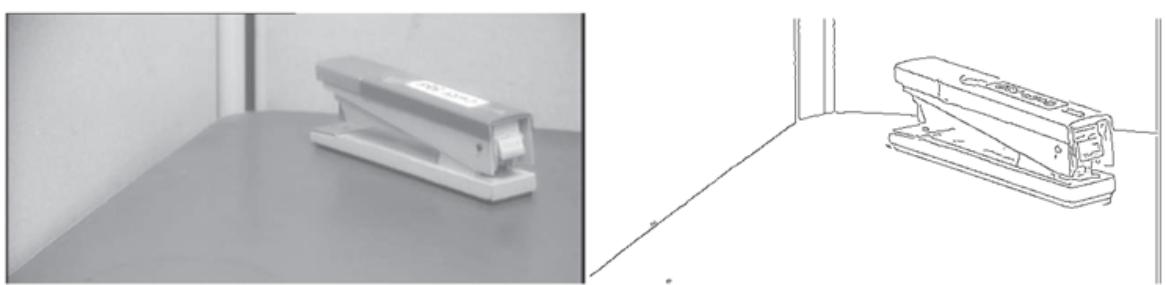
1. Photograph of a stapler. (b) Edges computed from (a).

25.3.2 Texture

In everyday language, the texture of surfaces hints at what they feel like when you run a finger over them (the words “texture,” “textile,” and “text” have the same Latin root, a word for weaving). In computational vision, texture refers to a pattern on a surface that can be sensed visually. Usually, these patterns are roughly regular. Examples include the pattern of windows on a building, the stitches on a sweater, the spots on a leopard’s skin, blades of grass on a lawn, pebbles on a beach, and a crowd of people in a stadium.

Texture

Sometimes the arrangement is quite periodic, as in the stitches on a sweater; in other instances, such as pebbles on a beach, the regularity is only in a statistical sense: the density of pebbles is roughly the same on different parts of the beach. A usual rough model of texture is a repetitive pattern of elements, sometimes called texels. This model is quite useful because it is surprisingly hard to make or find real textures that never repeat.

Texels

Texture is a property of an image patch, rather than a pixel in isolation. A good description of a patch’s texture should summarize what the patch looks like. The description should not change when the lighting changes. This rules out using edge points; if a texture is brightly lit, many locations within the patch will have high contrast and will generate edge points; but if the same texture is viewed under less bright light, many of these edges will not be above the threshold. The description should change in a sensible way when the patch rotates. It is important to preserve the difference between vertical stripes and horizontal stripes but not if the vertical stripes are rotated to the horizontal.

Texture representations with these properties have been shown to be useful for two key tasks. The first is identifying objects—a zebra and horse have similar shape, but different textures. The second is matching patches in one image to patches in another image, a key step in recovering 3D information from multiple images (Section 25.6.1 ).

Here is a basic construction for a texture representation. Given an image patch, compute the gradient orientation at each pixel in the patch, and then characterize the patch by a histogram of orientations. Gradient orientations are largely invariant to changes in illumination (the gradient will get longer, but it will not change direction). The histogram of orientations seems to capture important aspects of the texture. For example, vertical stripes will have two peaks in the histogram (one for the left side of each stripe and one for the right); leopard spots will have more uniformly distributed orientations.

But we do not know how big a patch to describe. There are two strategies. In specialized applications, image information reveals how big the patch should be (for example, one might grow a patch full of stripes until it covers the zebra). An alternative is to describe a patch centered at each pixel for a range of scales. This range usually runs from a few pixels to the extent of the image. Now divide the patch into bins, and in each bin construct an orientation histogram, then summarize the pattern of histograms across bins. It is no longer usual to construct these descriptions by hand. Instead, convolutional neural networks are used to produce texture representations. But the representations constructed by the networks seem to mirror this construction very roughly.

25.3.3 Optical flow

Next, let us consider what happens when we have a video sequence, instead of just a single static image. Whenever there is relative movement between the camera and one or more objects in the scene, the resulting apparent motion in the image is called optical flow. This describes the direction and speed of motion of features in the image as a result of relative motion between the viewer and the scene. For example, distant objects viewed from a moving car have much slower apparent motion than nearby objects, so the rate of apparent motion can tell us something about distance.

Optical flow

In Figure 25.9 we show two frames from a video of a tennis player. On the right we display the optical flow vectors computed from these images. The optical flow encodes useful information about scene structure—the tennis player is moving and the background (largely) isn’t. Furthermore, the flow vectors reveal something about what the player is doing—one arm and one leg are moving fast, and the other body parts aren’t.

Figure 25.9

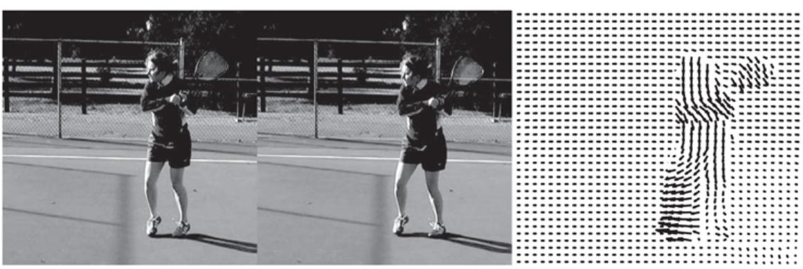
Two frames of a video sequence and the optical flow field corresponding to the displacement from one frame to the other. Note how the movement of the tennis racket and the front leg is captured by the directions of the arrows.

(Images courtesy of Thomas Brox.)

The optical flow vector field can be represented by its components in the direction and in the direction. To measure optical flow, we need to find corresponding points between one time frame and the next. A very simple-minded technique is based on the fact that image patches around corresponding points have similar intensity patterns. Consider a block of pixels centered at pixel , at time . This block of pixels is to be compared with pixel blocks centered at various candidate pixels at at time One possible measure of similarity is the sum of squared differences (SSD):

\[\text{SSD}(D\_x, D\_y) = \sum\_{(x, y)} \left( I(x, y, t) - I(x + D\_x, y + D\_y, t + D\_t) \right)^2.\]

Sum of squared differences (SSD)

Here, ranges over pixels in the block centered at . We find the that minimizes the SSD. The optical flow at is then . Note that for this to work, there should be some texture in the scene, resulting in windows containing a significant variation in brightness among the pixels. If one is looking at a uniform white wall, then the SSD is going to be nearly the same for the different candidate matches , and the algorithm is reduced to making a blind guess. The best-performing algorithms for measuring optical flow rely on a variety of additional constraints to deal with situations in which the scene is only partially textured.

25.3.4 Segmentation of natural images

Segmentation is the process of breaking an image into groups of similar pixels. The basic idea is that each image pixel can be associated with certain visual properties, such as brightness, color, and texture. Within an object, or a single part of an object, these attributes vary relatively little, whereas across an inter-object boundary there is typically a large change in one or more of these attributes. We need to find a partition of the image into sets of pixels such that these constraints are satisfied as well as possible. Notice that it isn’t enough just to find edges, because many edges are not object boundaries. So, for example, a tiger in grass may generate an edge on each side of each stripe and each blade of grass. In all the confusing edge data, we may miss the tiger for the stripes.

Segmentation

There are two ways of studying the problem, one focusing on detecting the boundaries of these groups, and the other on detecting the groups themselves, called regions. We illustrate this in Figure 25.10 , showing boundary detection in (b) and region extraction in (c) and (d).

Figure 25.10

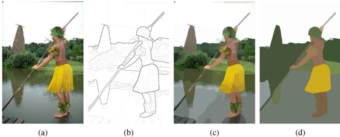
1. Original image. (b) Boundary contours, where the higher the value, the darker the contour. (c) Segmentation into regions, corresponding to a fine partition of the image. Regions are rendered in their mean colors. (d) Segmentation into regions, corresponding to a coarser partition of the image, resulting in fewer regions.

(Images courtesy of Pablo Arbelaez, Michael Maire, Charless Fowlkes and Jitendra Malik.)

Regions

One way to formalize the problem of detecting boundary curves is as a classification problem, amenable to the techniques of machine learning. A boundary curve at pixel location will have an orientation . An image neighborhood centered at looks roughly like a disk, cut into two halves by a diameter oriented at . We can compute the probability that there is a boundary curve at that pixel along that orientation by comparing features in the two halves. The natural way to predict this probability is to train a machine learning classifier using a data set of natural images in which humans have marked the ground truth boundaries—the goal of the classifier is to mark exactly those boundaries marked by humans and no others.

Boundaries detected by this technique are better than those found using the simple edge detection technique described previously. But there are still two limitations: (1) the boundary pixels formed by thresholding are not guaranteed to form closed curves, so this approach doesn’t deliver regions, and (2) the decision making exploits only local context, and does not use global consistency constraints.

The alternative approach is based on trying to “cluster” the pixels into regions based on their brightness, color and texture properties. There are a number of different ways in which this intuition can be formalized mathematically. For instance, Shi and Malik (2000) set this up as a graph partitioning problem. The nodes of the graph correspond to pixels, and edges to connections between pixels. The weight on the edge connecting a pair of pixels and is based on how similar the two pixels are in brightness, color, texture, etc. They then find partitions that minimize a normalized cut criterion. Roughly speaking, the criterion for partitioning the graph is to minimize the sum of weights of connections across the groups and maximize the sum of weights of connections within the groups.

It turns out that the approaches based on finding boundaries and on finding regions can be coupled, but we will not explore these possibilities here. Segmentation based purely on lowlevel, local attributes such as brightness and color can not be expected to deliver the final correct boundaries of all the objects in the scene. To reliably find boundaries associated with objects, it is also necessary to incorporate high-level knowledge of the kinds of objects one may expect to encounter in a scene. At this time, a popular strategy is to produce an over-segmentation of an image, where one is guaranteed not to have missed marking any of the true boundaries but may have marked many extra false boundaries as well. The resulting regions, called superpixels, provide a significant reduction in computational complexity for various algorithms, as the number of superpixels may be in the hundreds, compared to millions of raw pixels. Exploiting high-level knowledge of objects is the subject of the next section, and actually detecting the objects in images is the subject of Section 25.5 .

25.4 Classifying Images

Image classification applies to two main cases. In one, the images are of objects, taken from a given taxonomy of classes, and there’s not much else of significance in the picture—for example, a catalog of clothing or furniture images, where the background doesn’t matter, and the output of the classifier is “cashmere sweater” or “desk chair.”

In the other case, each image shows a scene containing multiple objects. So in grassland you might see a giraffe and a lion, and in the living room you might see a couch and lamp, but you don’t expect a giraffe or a submarine in a living room. We now have methods for largescale image classification that can accurately output “grassland” or “living room.”

Appearance

Modern systems classify images using appearance (i.e., color and texture, as opposed to geometry). There are two difficulties. First, different instances of the same class could look different—some cats are black and others are orange. Second, the same cat could look different at different times depending on several effects, (as illustrated in Figure 25.11 ):

• LIGHTING, which changes the brightness and color of the image.
• FORESHORTENING, which causes a pattern viewed at a glancing angle to be distorted.
• ASPECT, which causes objects to look different when seen from different directions. A doughnut seen from the side looks like a flattened oval, but from above it is an annulus.
• OCCLUSION, where some parts of the object are hidden. Objects can occlude one another, or parts of an object can occlude other parts, an effect known as self-occlusion.
• DEFORMATION, where the object changes its shape. For example, the tennis player moves her arms and legs.

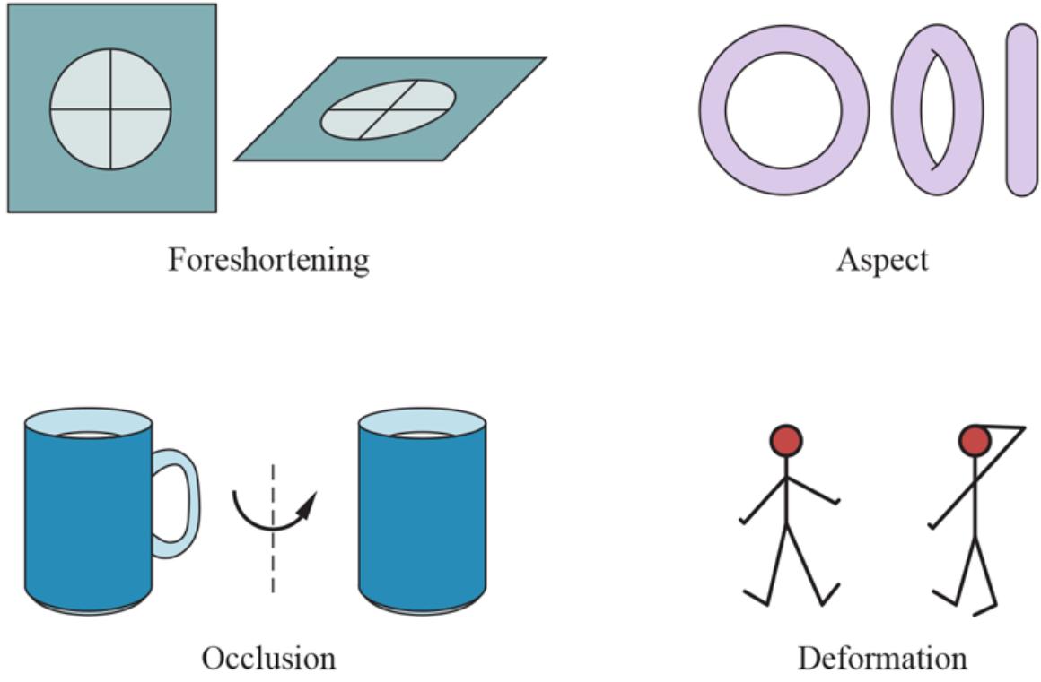
Important sources of appearance variation that can make different images of the same object look different. First, elements can foreshorten, like the circular patch on the top left. This patch is viewed at a glancing angle, and so is elliptical in the image. Second, objects viewed from different directions can change shape quite dramatically, a phenomenon known as aspect. On the top right are three different aspects of a doughnut. Occlusion causes the handle of the mug on the bottom left to disappear when the mug is rotated. In this case, because the body and handle belong to the same mug, we have selfocclusion. Finally, on the bottom right, some objects can deform dramatically.

Modern methods deal with these problems by learning representations and classifiers from very large quantities of training data using a convolutional neural network. With a sufficiently rich training set the classifier will have seen any effect of importance many times in training, and so can adjust for the effect.

25.4.1 Image classification with convolutional neural networks

Convolutional neural networks (CNNs) are spectacularly successful image classifiers. With enough training data and enough training ingenuity, CNNs produce very successful classification systems, much better than anyone has been able to produce with other methods.

The ImageNet data set played a historic role in the development of image classification systems by providing them with over 14 million training images, classified into over 30,000 fine-grained categories. ImageNet also spurred progress with an annual competition.

Systems are evaluated by both the classification accuracy of their single best guess and by top-5 accuracy, in which systems are allowed to submit five guesses—for example, malamute, husky, akita, samoyed, eskimo dog. ImageNet has 189 subcategories of dog, so even dog-loving humans find it hard to label images correctly with a single guess.

In the first ImageNet competition in 2010, systems could do no better than 70% top-5 accuracy. The introduction of convolutional neural networks in 2012 and their subsequent refinement led to an accuracy of 98% in top-5 (surpassing human performance) and 87% in top-1 accuracy by 2019. The primary reason for this success seems to be that the features that are being used by CNN classifiers are learned from data, not hand-crafted by a researcher; this ensures that the features are actually useful for classification.

Progress in image classification has been rapid because of the availability of large, challenging data sets such as ImageNet; because of competitions based on these data sets that are fair and open; and because of the widespread dissemination of successful models. The winners of competitions publish the code and often the pretrained parameters of their models, making it easy for others to fiddle with successful architectures and try to make them better.

25.4.2 Why convolutional neural networks classify images well

Image classification is best understood by looking at data sets, but ImageNet is much too large to look at in detail. The MNIST data set is a collection of 70,000 images of handwritten digits, 0–9, which is often used as a standard warmup data set. Looking at this data set (some examples appear in Figure 25.12 ) exposes some important, quite general, properties. You can take an image of a digit and make a number of small alterations without changing the identity of the digit: you can shift it, rotate it, make it brighter or darker, smaller or larger. This means that individual pixel values are not particularly informative we know that an 8 should have some dark pixels in the center and a 0 should not, but those dark pixels will be in slightly different pixel locations in each instance of an 8.

Figure 25.12

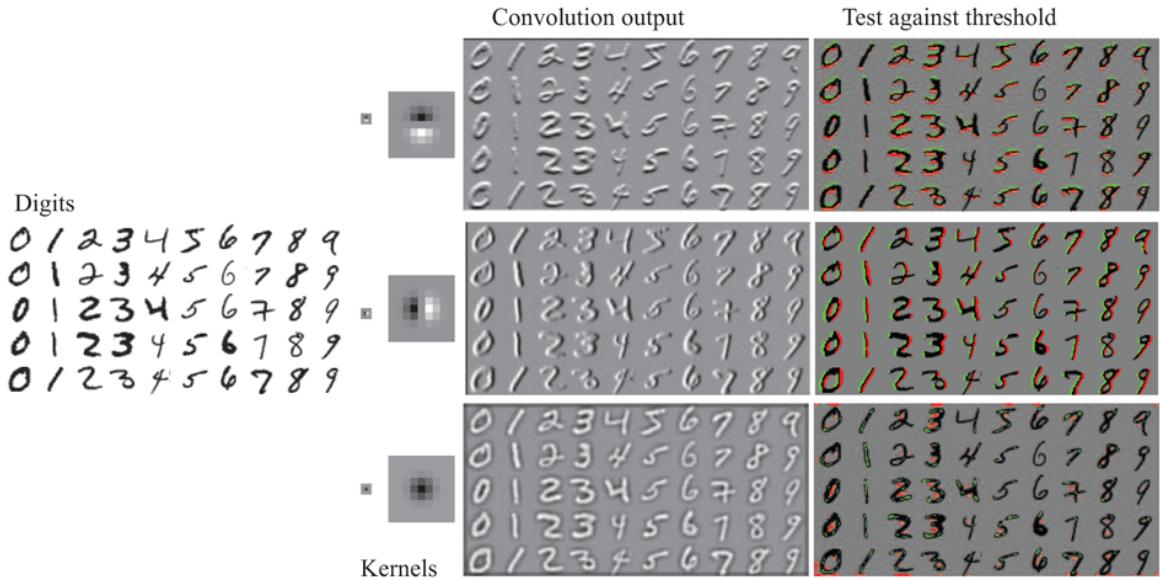
On the far left, some images from the MNIST data set. Three kernels appear on the center left. They are shown at actual size (tiny blocks) and magnified to reveal their content: mid-grey is zero, light is positive, and dark is negative. Center right shows the results of applying these kernels to the images. Right shows pixels where the response is bigger than a threshold (green) or smaller than a threshold (red). You should notice that this gives (from top to bottom): a horizontal bar detector; a vertical bar detector; and (harder to note) a line ending detector. These detectors pay attention to the contrast of the bar, so (for example) a horizontal bar that is light on top and dark below produces a positive (green) response, and one that is dark on top and light below gets a negative (red) response. These detectors are moderately effective, but not perfect.

Another important property of images is that local patterns can be quite informative: The digits 0, 6, 8 and 9 have loops; the digits 4 and 8 have crossings; the digits 1, 2, 3, 5 and 7 have line endings, but no loops or crossings; the digits 6 and 9 have loops and line endings. Furthermore, spatial relations between local patterns are informative. A 1 has two line endings above one another; a 6 has a line ending above a loop. These observations suggest a strategy that is a central tenet of modern computer vision: you construct features that respond to patterns in small, localized neighborhoods; then other features look at patterns of those features; then others look at patterns of those, and so on.

This is what convolutional neural networks do well. You should think of a layer—a convolution followed by a ReLU activation function—as a local pattern detector (Figure 25.12 ). The convolution measures how much each local window of the image looks like the kernel pattern; the ReLU sets low-scoring windows to zero, and emphasizes highscoring windows. So convolution with multiple kernels finds multiple patterns; furthermore, composite patterns can be detected by applying another layer to the output of the first layer.

Think about the output of the first convolutional layer. Each location receives inputs from pixels in a window about that location. The output of the ReLU, as we have seen, forms a simple pattern detector. Now if we put a second layer on top of this, each location in the second layer receives inputs from first-layer values in a window about that location. This means that locations in the second layer are affected by a larger window of pixels than those in the first layer. You should think of these as representing “patterns of patterns.” If we place a third layer on top of the second layer, locations in that third layer will depend on an even larger window of pixels; a fourth layer will depend on a yet larger window, and so on. The network is creating patterns at multiple levels, and is doing that by learning from the data rather than having the patterns given to it by a programmer.

While training a CNN “out of the box” does sometimes work, it helps to know a few practical techniques. One of the most important is data set augmentation, in which training examples are copied and modified slightly. For example, one might randomly shift, rotate, or stretch an image by a small amount, or randomly shift the hue of the pixels by a small amount. Introducing this simulated variation in viewpoint or lighting to the data set helps to increase the size of the data set, though of course the new examples are highly correlated with the originals. It is also possible to use augmentation at test time rather than training time. In this approach, the image is replicated and modified several times (e.g., with random cropping) and the classifier is run on each of the modified images. The outputs of the classifier from each copy are then used to vote for a final decision on the overall class.

Data set augmentation

When you are classifying images of scenes, every pixel could be helpful. But when you are classifying images of objects, some pixels aren’t part of the object, and so might be a distraction. For example, if a cat is lying on a dog bed, we want a classifier to concentrate on the pixels of the cat, not the bed. Modern image classifiers handle this well, classifying an image as “cat” accurately even if few pixels actually lie on the cat. There are two reasons for this. First, CNN-based classifiers are good at ignoring patterns that aren’t discriminative. Second, patterns that lie off the object might be discriminative (e.g., a cat toy, a collar with a little bell, or a dish of cat food might actually help tell that we are looking at a cat). This

effect is known as context. Context can help or can hurt, depending quite strongly on the particular data set and application.

Context

25.5 Detecting Objects

Image classifiers predict what is in the image—they classify the whole image as belonging to one class. Object detectors find multiple objects in an image, report what class each object is, and also report where each object is by giving a bounding box around the object. The set of classes is fixed in advance. So we might try to detect all faces, all cars, or all cats. 1

1 We will use the term “box” to mean any axis-aligned rectangular region of the image, and the term “window” mostly as a synonym for “box,” but with the connotation that we have a window onto the input where we are hoping to see something, and a bounding box in the output when we have found it.

Bounding box

Sliding window

We can build an object detector by looking at a small sliding window onto the larger image —a rectangle. At each spot, we classify what we see in the window, using a CNN classifier. We then take the high-scoring classifications—a cat over here and a dog over there—and ignore the other windows. After some work resolving conflicts, we have a final set of objects with their locations. There are still some details to work out:

• DECIDE ON A WINDOW SHAPE: The easiest choice by far is to use axis-aligned rectangles. (The alternative—some form of mask that cuts the object out of the image—is hardly ever used, because it is hard to represent and to compute with.) We still need to choose the width and height of the rectangles.
• BUILD A CLASSIFIER FOR WINDOWS: We already know how to do this with a CNN.
• DECIDE WHICH WINDOWS TO LOOK AT: Out of all possible windows, we want to select ones that are likely to have interesting objects in them.
• CHOOSE WHICH WINDOWS TO REPORT: Windows will overlap, and we don’t want to report the same object multiple times in slightly different windows. Some objects are not worth mentioning; think about the number of chairs and people in a picture of a large packed lecture hall. Should they all be reported as individual objects? Perhaps only the objects that appear large in the image—the front row—should be reported. The choice depends on the intended use of the object detector.
• REPORT PRECISE LOCATIONS OF OBJECTS USING THESE WINDOWS: Once we know that the object is somewhere in the window, we can afford to do more computation to figure out a more precise location within the window.

Let’s look more carefully at the problem of deciding which windows to look at. Searching all possible windows isn’t efficient—in an pixel image there are possible rectangular windows. But we know that windows that contain objects tend to have quite coherent color and texture. On the other hand, windows that cut an object in half have regions or edges that cross the side of the window. So it makes sense to have a mechanism that scores “objectness”—whether a box has an object in it, independent of what that object is. We can find the boxes that look like they have an object in them, and then classify the object for just those boxes that pass the objectness test.

A network that finds regions with objects is called a regional proposal network (RPN). The object detector known as Faster RCNN encodes a large collection of bounding boxes as a map of fixed size. Then it builds a network that can predict a score for each box, and trains this network so the score is large when the box contains an object, and small otherwise. Encoding boxes as a map is straightforward. We consider boxes centered on points throughout the image; we don’t need to consider every possible point (because moving by one pixel is not likely to change the classification); a good choice is a stride (the offset between center points) of 16 pixels. For each center point we consider several possible boxes, called anchor boxes. Faster RCNN uses nine boxes: small, medium, and large sizes; and tall, wide, and square aspect ratios.

Regional proposal network (RPN)

In terms of the neural network architecture, construct a 3D block where each spatial location in the block has two dimensions for the center point and one dimension for the type of box. Now any box with a good enough objectness score is called a region of interest (ROI), and must be checked by a classifier. But CNN classifiers prefer images of fixed size, and the boxes that pass the objectness test will differ in size and shape. We can’t make the boxes have the same number of pixels, but we can make them have the same number of features by sampling the pixels to extract features, a process called ROI pooling. This fixed-size feature map is then passed to the classifier.

Now for the problem of deciding which windows to report. Assume we look at windows of size with a stride of 1: each window is offset by just one pixel from the one before. There will be many windows that are similar, and should have similar scores. If they all have a score above threshold we don’t want to report all of them, because they very likely all refer to slightly different views of the same object. On the other hand if the stride is too large, it might be that an object is not contained within any one window, and will be missed. Instead, we can use a greedy algorithm called non-maximum suppression. First, build a sorted list of all windows with scores over a threshold. Then, while there are windows in the list, choose the window with the highest score and accept it as containing an object; discard from the list all other largely overlapping windows.

Non-maximum suppression

Finally, we have the problem of reporting the precise location of objects. Assume we have a window that has a high score, and has passed through non-maximum suppression. This window is unlikely to be in exactly the right place (remember, we looked at a relatively small number of windows with a small number of possible sizes). We use the feature representation computed by the classifier to predict improvements that will trim the window down to a proper bounding box, a step known as bounding box regression.

Bounding box regression

Evaluating object detectors takes care. First we need a test set: a collection of images with each object in the image marked by a ground truth category label and bounding box. Usually, the boxes and labels are supplied by humans. Then we feed each image to the object detector and compare its output to the ground truth. We should be willing to accept boxes that are off by a few pixels, because the ground truth boxes won’t be perfect. The evaluation score should balance recall (finding all the objects that are there) and precision (not finding objects that are not there).

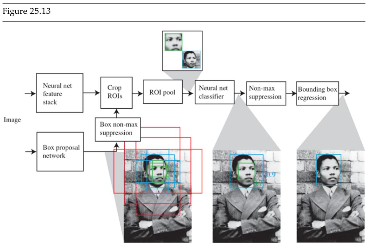
Faster RCNN uses two networks. A picture of a young Nelson Mandela is fed into the object detector. One network computes “objectness” scores of candidate image boxes, called “anchor boxes,” centered at a grid point. There are nine anchor boxes (three scales, three aspect ratios) at each grid point. For the example image, an inner green box and an outer blue box have passed the objectness test. The second network is a feature stack that computes a representation of the image suitable for classification. The boxes with highest objectness score are cut from the feature map, standardized in size with ROI pooling, and passed to a classifier. The blue box has a higher score than the green box and overlaps it, so the green box is rejected by non-maximum suppression. Finally, bounding box regression the blue box so that it fits the face. This means that the relatively coarse sampling of locations, scales, and aspect ratios does not weaken accuracy.

Photo by Sipa/Shutterstock.

25.6 The 3D World

Images show a 2D picture of a 3D world. But this 2D picture is rich with cues about the 3D world. One kind of cue occurs when we have multiple pictures of the same world, and can match points between pictures. Another kind of cue is available within a single picture.

25.6.1 3D cues from multiple views

Two pictures of objects in a 3D world are better than one for several reasons:

• If you have two images of the same scene taken from different viewpoints and you know enough about the two cameras, you can construct a 3D model—a collection of points with their coordinates in 3 dimensions—by figuring out which point in the first view corresponds to which point in the second view and applying some geometry. This is true for almost all pairs of viewing directions and almost all kinds of camera.
• If you have two views of enough points, and you know which point in the first view corresponds to which point in the second view, you do not need to know much about the cameras to construct a 3D model. Two views of two points gives you four coordinates, and you only need three coordinates to specify a point in 3D space; the extra coordinate comes in helpful to figure out what you need to know about the cameras. This is true for almost all pairs of viewing directions and almost all kinds of camera.

The key problem is to establish which point in the first view corresponds to which in the second view. Detailed descriptions of the local appearance of a point using simple texture features (like those in section 25.3.2 ) are often enough to match points. For example, in a scene of traffic on a street, there might be only one green light visible in two images taken of the scene; we can then hypothesize that these correspond to each other. The geometry of multiple camera views is very well understood (but sadly too complicated to expound here). The theory produces geometric constraints on which point in one image can match with which point in the other. Other constraints can be obtained by reasoning about the smoothness of the reconstructed surfaces.

There are two ways of getting multiple views of a scene. One is to have two cameras or two eyes (section 25.6.2 ). Another is to move (section 25.6.3 ). If you have more than two views, you can recover both the geometry of the world and the details of the view very accurately. Section 25.7.3 discusses some applications for this technology.

25.6.2 Binocular stereopsis

Most vertebrates have two eyes. This is useful for redundancy in case of a lost eye, but it helps in other ways too. Most prey have eyes on the side of the head to enable a wider field of vision. Predators have the eyes in the front, enabling them to use binocular stereopsis. Hold both index fingers up in front of your face, with one eye closed, and adjust them so the front finger occludes the other finger in the open eye’s view. Now swap eyes; you should notice that the fingers have shifted position with respect to one another. This shifting of position from left view to right view is known as disparity. In the right choice of coordinate system, if we superimpose left and right images of an object at some depth, the object shifts horizontally in the superimposed image, and the size of the shift is the reciprocal of the depth. You can see this in Figure 25.14 , where the nearest point of the pyramid is shifted to the left in the right image and to the right in the left image.

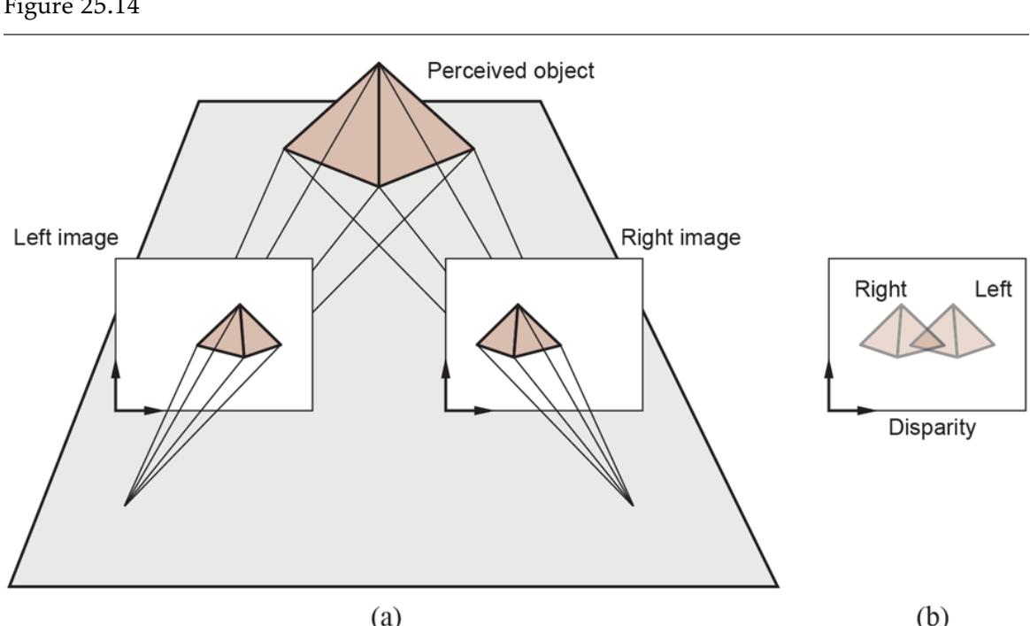
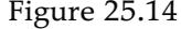
Translating a camera parallel to the image plane causes image features to move in the camera plane. The disparity in positions that results is a cue to depth. If we superimpose left and right images, as in (b), we see the disparity.

Binocular stereopsis

Disparity

To measure disparity we need to solve the correspondence problem—to determine for a point in the left image, its “partner” in the right image which results from the projection of the same scene point. This is analogous to what is done in measuring optical flow, and the most simple-minded approaches are somewhat similar. These methods search for blocks of left and right pixels that match, using the sum of squared differences (as in Section 25.3.3 ). More sophisticated methods use more detailed texture representations of blocks of pixels (as in Section 25.3.2 ). In practice, we use much more sophisticated algorithms, which exploit additional constraints.

Baseline

Assuming that we can measure disparity, how does this yield information about depth in the scene? We will need to work out the geometrical relationship between disparity and depth. We will consider first the case when both the eyes (or cameras) are looking forward with their optical axes parallel. The relationship of the right camera to the left camera is then just a displacement along the -axis by an amount , the baseline. We can use the optical flow equations from Section 25.3.3 , if we think of this as resulting from a translation vector acting for time , with and . The horizontal and vertical disparity are given by the optical flow components, multiplied by the time step Carrying out the substitutions, we get the result that . In other words, the horizontal disparity is equal to the ratio of the baseline to the depth, and the vertical disparity is zero. We can recover the depth given that we know , and can measure .

Under normal viewing conditions, humans fixate; that is, there is some point in the scene at which the optical axes of the two eyes intersect. Figure 25.15 shows two eyes fixated at a point , which is at a distance from the midpoint of the eyes. For convenience, we will compute the angular disparity, measured in radians. The disparity at the point of fixation is zero. For some other point in the scene that is farther away, we can compute the angular displacements of the left and right images of , which we will call and , respectively. If each of these is displaced by an angle relative to , then the displacement between and , which is the disparity of , is just . From Figure 25.15 , and , but for small angles, , so

\[ \delta\theta/2 = \frac{b/2}{Z} - \frac{b/2}{Z + \delta Z} \approx \frac{b\delta Z}{2Z^2} \]

The relation between disparity and depth in stereopsis. The centers of projection of the two eyes are distance apart, and the optical axes intersect at the fixation point . The point in the scene projects to points and in the two eyes. In angular terms, the disparity between these is (the diagram shows two angles of ).

Fixate

and, since the actual disparity is , we have

\[\text{disparity} = \frac{b\delta Z}{Z^2}\]

In humans, the baseline is about 6 cm. Suppose that is about 100 cm and that the smallest detectable (corresponding to the size of a single pixel) is about 5 seconds of arc, giving a of 0.4 mm. For cm, we get the impressively small value . That is, at a distance of 30 cm, humans can discriminate depths that differ by as little as 0.036 mm, enabling us to thread needles and the like.

25.6.3 3D cues from a moving camera

Assume we have a camera moving in a scene. Take Figure 25.14 and label the left image “Time” and the right image “Time”. The geometry has not changed, so all the material from the discussion of stereopsis also applies when a camera moves. What we called disparity in that section is now thought of as apparent motion in the image, and called optical flow. This is a source of information for both the movement of the camera and the geometry of the scene. To understand this, we state (without proof) an equation that relates the optical flow to the viewer’s translational velocity and the depth in the scene.

The optical flow field is a vector field of velocities in the image, . Expressions for these components, in a coordinate frame centered on the camera and assuming a focal length of , are

\[v\_x(x,y) = \frac{-T\_x + xT\_z}{Z(x,y)} \text{ and } \qquad v\_y(x,y) = \frac{-T\_y + yT\_z}{Z(x,y)}\]

where is the -coordinate (that is, depth) of the point in the scene corresponding to the point in the image at .

Note that both components of the optical flow, and , are zero at the point . This point is called the focus of expansion of the flow field. Suppose we change the origin in the – plane to lie at the focus of expansion; then the expressions for optical flow take on a particularly simple form. Let be the new coordinates defined by . Then

\[v\_x(x',y') = \frac{x''T\_z}{Z(x',y')}, \qquad v\_y(x',y') = \frac{y'T\_z}{Z(x',y')}\]

Focus of expansion

Note that there is a scale factor ambiguity here (which is why assuming a focal length of is harmless). If the camera was moving twice as fast, and every object in the scene was twice as big and at twice the distance to the camera, the optical flow field would be exactly the same. But we can still extract quite useful information.

• 1. Suppose you are a fly trying to land on a wall and you want useful information from the optical flow field. The optical flow field cannot tell you the distance to the wall or the velocity to the wall, because of the scale ambiguity. But if you divide the distance by the velocity, the scale ambiguity cancels. The result is the time to contact, given by , and is very useful indeed to control the landing approach. There is considerable experimental evidence that many different animal species exploit this cue.
• 2. Consider two points at depths respectively. We may not know the absolute value of either of these, but by considering the inverse of the ratio of the optical flow magnitudes at these points, we can determine the depth ratio . This is the cue of motion parallax, one we use when we look out of the side window of a moving car or train and infer that the slower-moving parts of the landscape are farther away.

25.6.4 3D cues from one view

Even a single image provides a rich collection of information about the 3D world. This is true even if the image is just a line drawing. Line drawings have fascinated vision scientists, because people have a sense of 3D shape and layout even though the drawing seems to contain very little information to choose from the vast collection of scenes that could produce the same drawing. Occlusion is one key source of information: if there is evidence in the picture that one object occludes another, then the occluding object is closer to the eye.

In images of real scenes, texture is a strong cue to 3D structure. Section 25.3.2 stated that texture is a repetitive pattern of texels. Although the distribution of texels may be uniform on objects in the scene—for example, pebbles on a beach—it may not be uniform in image the farther pebbles appear smaller than the nearer pebbles. As another example, think about a piece of polka-dot fabric. All the dots are the same size and shape on the fabric, but in a perspective view some dots are ellipses due to foreshortening. Modern methods exploit these cues by learning a mapping from images to 3D structure (Section 25.7.4 ), rather than reasoning directly about the underlying mathematics of texture.

Shading—variation in the intensity of light received from different portions of a surface in a scene—is determined by the geometry of the scene and by the reflectance properties of the surfaces. There is very good evidence that shading is a cue to 3D shape. The physical argument is easy. From the physical model of section 25.2.4 , we know that if a surface normal points toward the light source, the surface is brighter, and if it points away, the surface is darker. This argument gets more complicated if the reflectance of the surface isn’t known, and the illumination field isn’t even, but humans seem to be able to get a useful perception of shape from shading. We know frustratingly little about algorithms to do this.

If there is a familiar object in the picture, what it looks like depends very strongly on its pose, that is, its position and orientation with respect to the viewer. There are straightforward algorithms for recovering pose from correspondences between points on an object and points on a model of the object. Recovering the pose of a known object has many applications. For instance, in an industrial manipulation task, the robot arm cannot pick up an object until the pose is known. Robotic surgery applications depend on exactly computing the transformations between the camera’s position and the positions of the surgical tool and the patient (to yield the transformation from the tool’s position to the patient’s position).

Pose

Spatial relations between objects are another important cue. Here is an example. All pedestrians are about the same height, and they tend to stand on a ground plane. If we know where the horizon is in an image, we can rank pedestrians by distance to the camera. This works because we know where their feet are, and pedestrians whose feet are closer to the horizon in the image are farther away from the camera, and so must be smaller in the image. This means we can rule out some detector responses—if a detector finds a pedestrian who is large in the image and whose feet are close to the horizon, it has found an enormous pedestrian; these don’t exist, so the detector is wrong. In turn, a reasonably reliable pedestrian detector is capable of producing estimates of the horizon, if there are several pedestrians in the scene at different distances from the camera. This is because the relative scaling of the pedestrians is a cue to where the horizon is. So we can extract a horizon estimate from the detector, then use this estimate to prune the pedestrian detector’s mistakes.

25.7 Using Computer Vision

Here we survey a range of computer vision applications. There are now many reliable computer vision tools and toolkits, so the range of applications that are successful and useful is extraordinary. Many are developed at home by enthusiasts for special purposes, which is testimony to how usable the methods are and how much impact they have. (For example, an enthusiast created a great object-detection-based pet door that refuses entry to a cat if it is bringing in a dead mouse–a Web search will find it for you).

25.7.1 Understanding what people are doing

If we could build systems that understood what people are doing by analyzing video, we could build human-computer interfaces that watch people and react to their behavior. With these interfaces, we could: design buildings and public places better, by collecting and using data about what people do in public; build more accurate and less intrusive security surveillance systems; build automated sports commentators; make construction sites and workplaces safer by generating warnings when people and machines get dangerously close; build computer games that make a player get up and move around; and save energy by managing heat and light in a building to match where the occupants are and what they are doing.

The state of the art for some problems is now extremely strong. There are methods that can predict the locations of a person’s joints in an image very accurately. Quite good estimates of the 3D configuration of that person’s body follow (see Figure 25.16 ). This works because pictures of the body tend to have weak perspective effects, and body segments don’t vary much in length, so the foreshortening of a body segment in an image is a good cue to the angle between it and the camera plane. With a depth sensor, these estimates can be made fast enough to build them into computer game interfaces.

Figure 25.16

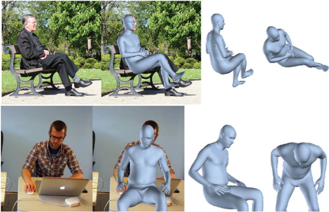
Reconstructing humans from a single image is now practical. Each row shows a reconstruction of 3D body shape obtained using a single image. These reconstructions are possible because methods can estimate the location of joints, the joint angles in 3D, the shape of the body, and the pose of the body with respect to an image. Each row shows the following: far left a picture; center left the picture with the reconstructed body superimposed; center right another view of the reconstructed body; and far right yet another view of the reconstructed body. The different views of the body make it much harder to conceal errors in reconstruction. Figure courtesy of Angjoo Kanazawa, produced by a system described in Kanazawa et al. (2018a).

Classifying what people are doing is harder. Video that shows rather structured behaviors, like ballet, gymnastics, or tai chi, where there are quite specific vocabularies that refer to very precisely delineated activities on simple backgrounds, is quite easy to deal with. Good results can be obtained with a lot of labeled data and an appropriate convolutional neural network. However, it can be difficult to prove that the methods actually work, because they rely so strongly on context. For example, a classifier that labels “swimming” sequences very well might just be a swimming pool detector, which wouldn’t work for (say) swimmers in rivers.

More general problems remain open—for example, how to link observations of the body and the objects nearby to the goals and intentions of the moving people. One source of difficulty is that similar behaviors look different, and different behaviors look similar, as Figure 25.17 shows.

Figure 25.17

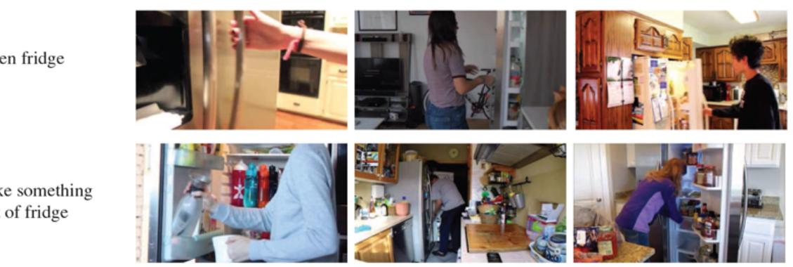
The same action can look very different; and different actions can look similar. These examples show actions taken from a data set of natural behaviors; the labels are chosen by the curators of the data set, rather than predicted by an algorithm. Top: examples of the label “opening fridge,” some shown in closeup and some from afar. Bottom: examples of the label “take something out of fridge.” Notice how in both rows the subject’s hand is close to the fridge door—telling the difference between the cases requires quite subtle judgment about where the hand is and where the door is. Figure courtesy of David Fouhey, taken from a data set described in Fouhey et al. (2018).

Another difficulty is caused by time scale. What someone is doing depends quite strongly on the time scale, as Figure 25.18 illustrates. Another important effect shown in that figure is that behavior composes—several recognized behaviors may be combined to form a single higher-level behavior such as fixing a snack.

Figure 25.18

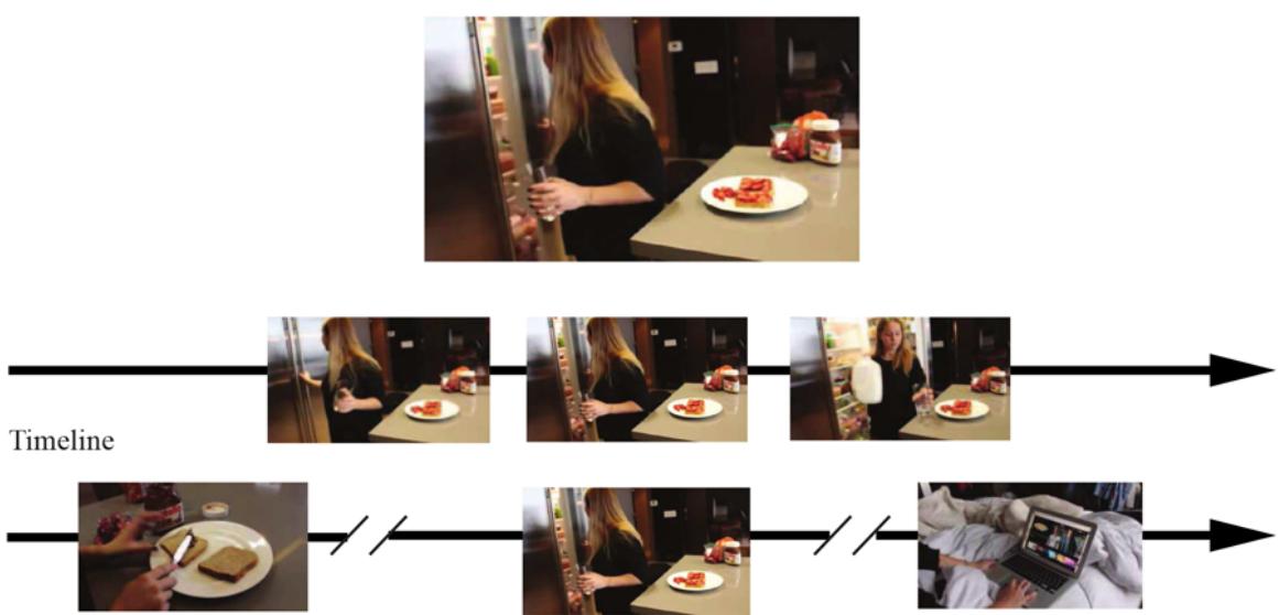
What you call an action depends on the time scale. The single frame at the top is best described as opening the fridge (you don’t gaze at the contents when you close a fridge). But if you look at a short clip of video (indicated by the frames in the center row), the action is best described as getting milk from the

fridge. If you look at a long clip (the frames in the bottom row), the action is best described as fixing a snack. Notice that this illustrates one way in which behavior composes: getting milk from the fridge is sometimes part of fixing a snack, and opening the fridge is usually part of getting milk from the fridge. Figure courtesy of David Fouhey, taken from a data set described in Fouhey et al. (2018).

It may also be that unrelated behaviors are going on at the same time, such as singing a song while fixing a snack. A challenge is that we don’t have a common vocabulary for the pieces of behavior. People tend to think they know a lot of behavior names but can’t produce long lists of such words on demand. That makes it harder to get data sets of consistently labeled behaviors.

Learned classifiers are guaranteed to behave well only if the training and test data come from the same distribution. We have no way of checking that this constraint applies to images, but empirically we observe that image classifiers and object detectors work very well. But for activity data, the relationship between training and test data is more untrustworthy because people do so many things in so many contexts. For example, suppose we have a pedestrian detector that performs well on a large data set. There will be rare phenomena (for example, people mounting unicycles) that do not appear in the training set, so we can’t say for sure how the detector will work in such cases. The challenge is to prove that the detector is safe whatever pedestrians do, which is difficult for current theories of learning.

25.7.2 Linking pictures and words

Many people create and share pictures and videos on the Internet. The difficulty is finding what you want. Typically, people want to search using words (rather than, say, example sketches). Because most pictures don’t come with words attached, it is natural to try and build tagging systems that tag images with relevant words. The underlying machinery is straightforward—we apply image classification and object detection methods and tag the image with the output words. But tags aren’t a comprehensive description of what is happening in an image. It matters who is doing what, and tags don’t capture this. For example, tagging a picture of a cat in the street with the object categories “cat”, “street”, “trash can” and “fish bones” leaves out the information that the cat is pulling the fish bones out of an open trash can on the street.

Tagging system

As an alternative to tagging, we might build captioning systems—systems that write a caption of one or more sentences describing the image. The underlying machinery is again straightforward—couple a convolutional network (to represent the image) to a recurrent neural network or transformer network (to generate sentences), and train the result with a data set of captioned images. There are many images with captions available on the Internet; curated data sets use human labor to augment each image with additional captions to capture the variation in natural language. For example, the COCO (Common Objects in Context) data set is a comprehensive collection of over 200,000 images labeled with five captions per image.

Captioning systems

Current methods for captioning use detectors to find a set of words that describe the image, and provide those words to a sequence model that is trained to generate a sentence. The most accurate methods search through the sentences that the model can generate to find the best, and strong methods appear to require a slow search. Sentences are evaluated with a set of scores that check whether the generated sentence (a) uses phrases common in the ground truth annotations and (b) doesn’t use other phrases. These scores are hard to use directly as a loss function, but reinforcement learning methods can be used to train networks that get very good scores. Often there will be an image in the training set whose description has the same set of words as an image in the test set; in that case a captioning system can just retrieve a valid caption rather than having to generate a new one. Caption writing systems produce a mix of excellent results and embarrassing errors (see Figure 25.19 ).

Automated image captioning systems produce some good results and some failures. The two captions at left describe the respective images well, although “eating … in his mouth” is a disfluency that is fairly typical of the recurrent neural network language models used by early captioning systems. For the two captions on the right, the captioning system seems not to know about squirrels, and so guesses the animal from context; it also fails to recognize that the two squirrels are eating. Image credits: geraine/Shutterstock; ESB Professional/Shutterstock; BushAlex/Shutterstock; Maria.Tem/Shutterstock. The images shown are similar but not identical to the original images from which the captions were generated. For the original images see Aneja et al. (2018).

Captioning systems can hide their ignorance by omitting to mention details they can’t get right or by using contextual cues to guess. For example, captioning systems tend to be poor at identifying the gender of people in images, and often guess based on training data statistics. That can lead to errors—men also like shopping and women also snowboard. One way to establish whether a system has a good representation of what is happening in an image is to force it to answer questions about the image. This is a visual question answering or VQA system. An alternative is a visual dialog system, which is given a picture, its caption, and a dialog. The system must then answer the last question in the dialog. As Figure 25.20 shows, vision remains extremely hard and VQA systems often make errors.

Figure 25.20

Visual question-answering systems produce answers (typically chosen from a multiple-choice set) to natural-language questions about images. Top: the system is producing quite sensible answers to rather difficult questions about the image. Bottom: less satisfactory answers. For example, the system is guessing about the number of holes in a pizza, because it doesn’t understand what counts as a hole, and it has real difficulty counting. Similarly, the system selects brown for the cat’s leg because the background is brown and it can’t localize the leg properly.

Image credits: (Top) Tobyanna/Shutterstock; 679411/Shutterstock; ESB Professional/Shutterstock; Africa Studio/Shutterstock; (Bottom) Stuart Russell; Maxisport/Shutterstock; Chendongshan/Shutterstock; Scott Biales DitchTheMap/Shutterstock. The images shown are similar but not identical to the original images to which the question-answering system was applied. For the original images see Goyal et al. (2017).

Visual question answering (VQA)

Visual dialog

25.7.3 Reconstruction from many views

Reconstructing a set of points from many views—which could come from video or from an aggregation of tourist photographs—is similar to reconstructing the points from two views, but there are some important differences. There is far more work to be done to establish correspondence between points in different views, and points can go in and out of view, making the matching and reconstruction process messier. But more views means more constraints on the reconstruction and on the recovered viewing parameters, so it is usually possible to produce extremely accurate estimates of both the position of the points and of the viewing parameters. Rather roughly, reconstruction proceeds by matching points over pairs of images, extending these matches to groups of images, coming up with a rough solution for both geometry and viewing parameters, then polishing that solution. Polishing means minimizing the error between points predicted by the model (of geometry and viewing parameters) and the locations of image features. The detailed procedures are too complex to cover fully, but are now very well understood and quite reliable.

All the geometric constraints on correspondences are known for any conceivably useful form of camera. The procedures can be generalized to deal with views that are not orthographic; to deal with points that are observed in only some views; to deal with

unknown camera parameters (like focal length); and to exploit various sophisticated searches for appropriate correspondences. It is practical to accurately reconstruct a model of an entire city from images. Some applications are:

• MODEL BUILDING: For example, one might build a modeling system that takes many views depicting an object and produces a very detailed 3D mesh of textured polygons for use in computer graphics and virtual reality applications. It is routine to build models like this from video, but such models can now be built from apparently random sets of pictures. For example, you can build a 3D model of the Statue of Liberty from pictures found on the Internet.
• MIX ANIMATION WITH LIVE ACTORS IN VIDEO: To place computer graphics characters into real video, we need to know how the camera moved for the real video, so we can render the character correctly, changing the view as the camera moves.
• PATH RECONSTRUCTION: Mobile robots need to know where they have been. If the robot has a camera, we can build a model of the camera’s path through the world; that will serve as a representation of the robot’s path.
• CONSTRUCTION MANAGEMENT: Buildings are enormously complicated artifacts, and keeping track of what is happening during construction is difficult and expensive. One way to keep track is to fly drones through the construction site once a week, filming the current state. Then build a 3D model of the current state and explore the difference between the plans and the reconstruction using visualization techniques. Figure 25.21 illustrates this application.

Figure 25.21

3D models of construction sites are produced from images by structure-from-motion and multiview stereo algorithms. They help construction companies to coordinate work on large buildings by comparing a 3D model of the actual construction to date with the building plans. Left: A

visualization of a geometric model captured by drones. The reconstructed 3D points are rendered in color, so the result looks like progress to date (note the partially completed building with crane). The small pyramids show the pose of a drone when it captured an image, to allow visualization of the flight path. Right: These systems are actually used by construction teams; this team views the model of the as-built site, and compares it with building plans as part of the coordination meeting. Figure courtesy of Derek Hoiem, Mani Golparvar-Fard and Reconstruct, produced by a commercial system described in a blog post at medium.com/reconstruct-inc.

25.7.4 Geometry from a single view

Geometric representations are particularly useful if you want tomove, because they can reveal where you are, where you can go, and what you are likely bump into. But it is not always convenient to use multiple views to produce a geometric model. For example, when you open the door and step into a room, your eyes are too close together to recover a good representation of the depth to distant objects across the room. You could move your head back and forth, but that is time-consuming and inconvenient.

An alternative is to predict a depth map—an array giving the depth to each pixel in the image, nominally from the camera—from a single image. For many kinds of scenes, this is surprisingly easy to do accurately, because the depth map has quite a simple structure. This is particularly true of rooms and indoor scenes in general. The mechanics are straightforward. One obtains a data set of images and depth maps, then trains a network to predict depth maps from images. A variety of interesting variations of the problem can be solved. The problem with a depth map is that it doesn’t tell you anything about the backs of objects, or the space behind the objects. But there are methods that can predict what voxels (3D pixels) are occupied by known objects (the object geometry is known) and what a depth map would look like if an object were removed (and so where you could hide objects). These methods work because object shapes are quite strongly stylized.

Depth map

As we saw in Section 25.6.4 , recovering the pose of a known object using a 3D model is straightforward. Now imagine you see a single image of, say, a sparrow. If you have seen many images of sparrow-like birds in the past, you can reconstruct a reasonable estimate of both the pose of the sparrow and its geometric model from that single image. Using the past images you build a small, parametric family of geometric models for sparrow-like birds; then an optimization procedure is used to find the best set of parameters and viewpoints to explain the image that you see. This argument works to supply texture for that model, too, even for the parts you cannot see (Figure 25.22 ).

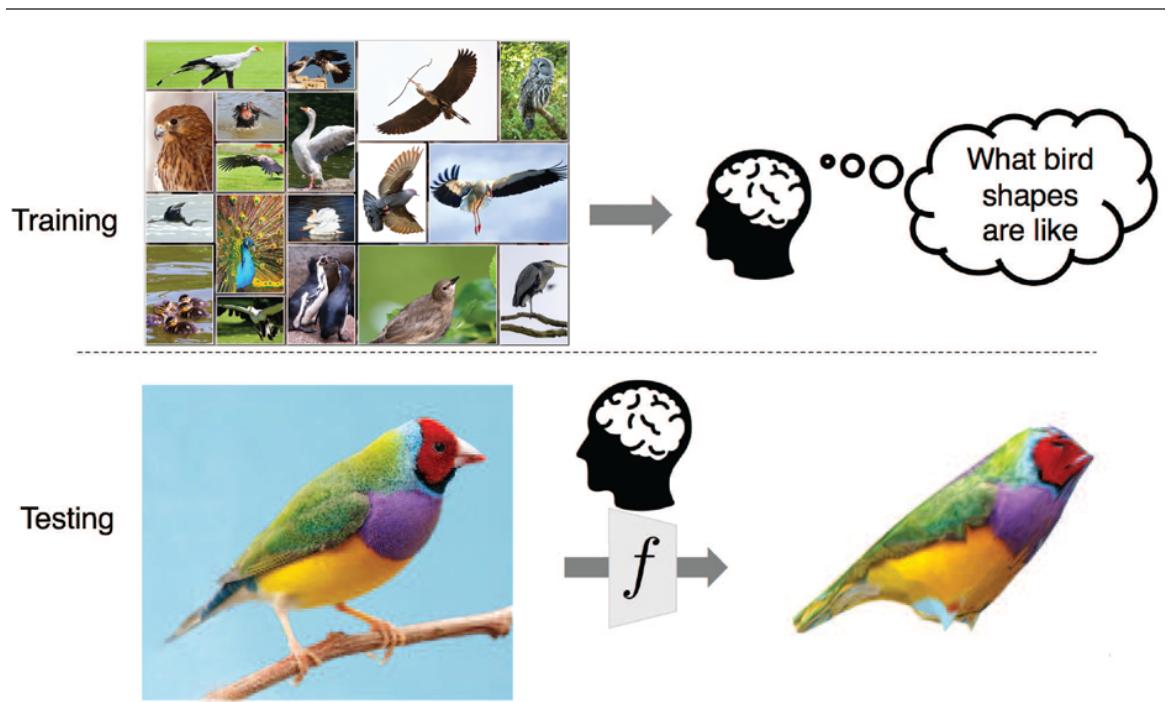
Figure 25.22

If you have seen many pictures of some category—say, birds (top)—you can use them to produce a 3D reconstruction from a single new view (bottom). You need to be sure that all objects have a fairly similar geometry (so a picture of an ostrich won’t help if you’re looking at a sparrow), but classification methods can sort this out. From the many images you can estimate how texture values in the image are distributed across the object, and thus complete the texture for parts of the bird you haven’t seen yet (bottom). Figure courtesy of Angjoo Kanazawa, produced by a system described in Kanazawa et al. (2018b).

Top photo credit: Satori/123RF; Bottom left credit: Four Oaks/Shutterstock.

25.7.5 Making pictures

It is now common to insert computer graphics models into photographs in a convincing fashion, as in Figure 25.23 , where a statue has been placed into a photo of a room. First estimate a depth map and albedo for the picture. Then estimate the lighting in the image by matching it to other images with known lighting. Place the object in the image’s depth map, and render the resulting world with a physical rendering program—a standard tool in computer graphics. Finally, blend the modified image with the original image.

Figure 25.23

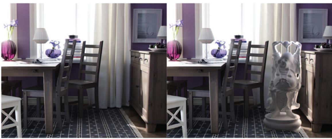
On the left, an image of a real scene. On the right, a computer graphics object has been inserted into the scene. You can see that the light appears to be coming from the right direction, and that the object seems to cast appropriate shadows. The generated image is convincing even if there are small errors in the lighting and shadows, because people are not expert at identifying these errors. Figure courtesy of Kevin Karsch, produced by a system described in Karsch et al. (2011)

Neural networks can also be trained to do image transformation: mapping images from type X—for example, a blurry image; an aerial image of a town; or a drawing of a new product—to images of type Y—for example, a deblurred version of the image; a road map; or a product photograph. This is easiest when the training data consists of (X, Y) pairs of images—in Figure 25.24 each example pair has an aerial image and the corresponding road map section. The training loss compares the output of the network with the desired output, and also has a loss component from a generative adversarial network (GAN) that ensures that the output has the right kinds of features for images of type Y. As we see in the test portion of Figure 25.24 , systems of this kind perform very well.

Figure 25.24

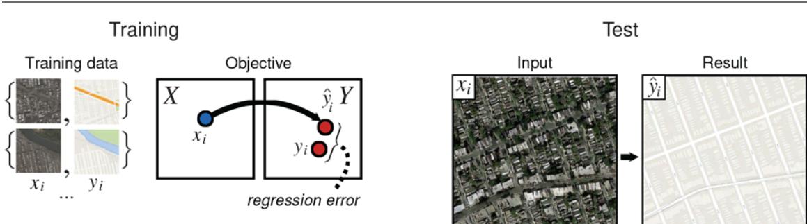
Paired image translation where the input consists of aerial images and the corresponding map tiles, and the goal is to train a network to produce a map tile from an aerial image. (The system can also learn to generate aerial images from map tiles.) The network is trained by comparing (the output for example of type ) to the right output of type . Then at test time, the network must make new images of type from new inputs of type . Figure courtesy of Phillip Isola, Jun-Yan Zhu and Alexei A. Efros, produced by a system described in Isola et al. (2017). Map data © 2019 Google.

Image transformation

Sometimes we don’t have images that are paired with each other, but we do have a big collection of images of type X (say, pictures of horses) and a separate collection of type Y (say, pictures of zebras). Imagine an artist who is tasked with creating an image of a zebra running in a field. The artist would appreciate being able to select just the right image of a horse, and then having the computer automatically transform the horse into a zebra (Figure 25.25 ). To achieve this we can train two transformation networks, with an additional constraint called a cycle constraint. The first network maps horses to zebras; the second network maps zebras to horses; and the cycle constraint requires that when you map X to Y to X (or Y to X to Y), you get what you started with. Again, GAN losses ensure that the horse (or zebra) pictures that the networks output are “like” real horse (or zebra) pictures.

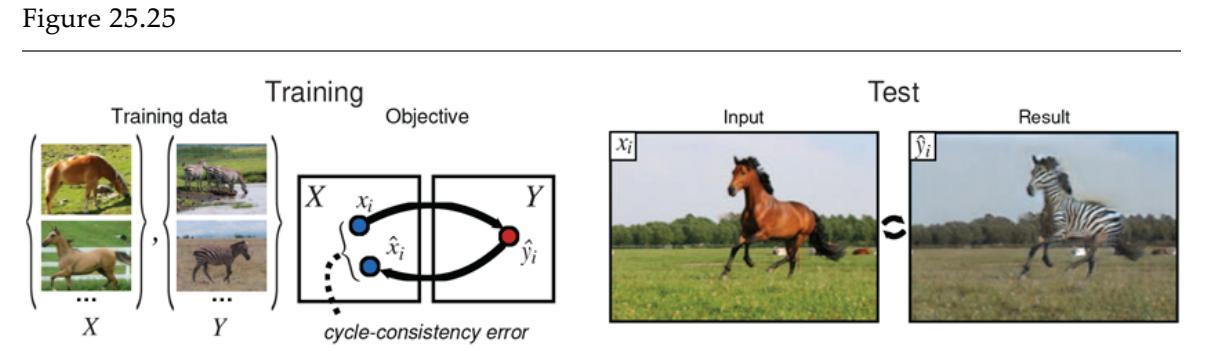
Unpaired image translation: given two populations of images (here type X is horses and type Y is zebras), but no corresponding pairs, learn to translate a horse into a zebra. The method trains two predictors: one that maps type X to type Y, and another that maps type Y to type X. If the first network maps a horse to a zebra , the second network should map back to the original . The difference between and is what trains the two networks. The cycle from Y to X and back must be closed. Such networks can successfully impose rich transformations on images.

Figure courtesy of Alexei A. Efros; see Zhu et al. (2017). Running horse photo by Justyna Furmanczyk Gibaszek/Shutterstock.

Another artistic effect is called style transfer: the input consists of two images—the content (for example, a photograph of a cat); and the style (for example, an abstract painting). The output is a version of the cat rendered in the abstract style (see Figure 25.26 ). The key insight to solving this problem is that if we examine a deep convolutional neural network (CNN) that has been trained to do object recognition (say, on ImageNet), we find that the early layers tend to represent the style of a picture, and the late layers represent the content. Let be the content image and be the style image, and let be the vector of activations of an early layer on image and be the vector of activations of a late layer on image . Then we want to generate some image that has similar content to the house photo, that is, minimizes and also has similar style to the impressionist painting, that is, minimizes We use gradient descent with a loss function that is a linear combination of these two factors to find an image that minimizes the loss.

Figure 25.26

Style transfer: The content of a photo of a cat is combined with the style of an abstract painting to yield a new image of the cat rendered in the abstract style (right). The painting is Wassily Kandinsky’s Lyrisches or The Lyrical (public domain); the cat is Cosmo.

Style transfer

Generative adversarial networks (GANs) can create novel photorealistic images, fooling most people most of the time. One kind of image is the deepfake—an image or video that looks like a particular person, but is generated from amodel. For example, when Carrie Fisher was 60, a generated replica of her 19-year-old face was superimposed on another actor’s body for the making of Rogue One. The movie industry creates ever-better deepfakes for artistic purposes, and researchers work on countermeasures for detecting deepfakes, to mitigate the destructive effects of fake news.

Deepfake

Generated images can also be used to maintain privacy. For example, there are image data sets in radiological practices that would be useful for researchers, but can’t be published because of patient confidentiality. Generative image models can take a private data set of images and produce a synthetic data set that can be shared with researchers. This data set should be (a) like the training data set; (b) different; and (c) controllable. Consider chest Xrays. The synthetic data set should be like the training data set in the sense that each image individually would fool a radiologist and the frequencies of each effect should be right, so a radiologist would not be surprised by how often (say) pneumonia appears. The new data set should be different, in the sense that it does not reveal personally identifiable information. The new data set should be controllable, so that the frequencies of effects can be adjusted to reflect the communities of interest. For example, pneumonias are more common in the elderly than in young adults. Each of these goals is technically difficult to reach, but image data sets have been created that fool practicing radiologists some of the time (Figure 25.27 ).

Figure 25.27

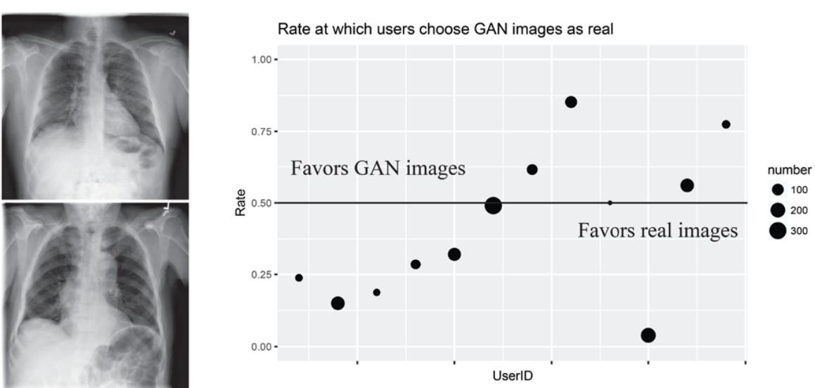
GAN generated images of lung X-rays. On the left, a pair consisting of a real X-ray and a GAN-generated X-ray. On the right, results of a test asking radiologists, given a pair of X-rays as seen on the left, to tell which is the real X-ray. On average, they chose correctly 61% of the time, somewhat better than chance. But they differed in their accuracy—the chart on the right shows the error rate for 12 different radiologists; one of them had an error rate near 0% and another had 80% errors. The size of each dot indicates the number of images each radiologist viewed. Figure courtesy of Alex Schwing, produced by a system described in Deshpande et al. (2019).

25.7.6 Controlling movement with vision

One of the principal uses of vision is to provide information both for manipulating objects picking them up, grasping them, twirling them, and so on—and for navigating while avoiding obstacles. The ability to use vision for these purposes is present in the most primitive of animal visual systems. In many cases, the visual system is minimal, in the sense that it extracts from the available light field just the information the animal needs to inform its behavior. Quite probably, modern vision systems evolved from early, primitive organisms that used a photosensitive spot at one end in order to orient themselves toward (or away from) the light. We saw in Section 25.6 that flies use a very simple optical flow detection system to land on walls.

Suppose that, rather than landing on walls, we want to build a self-driving car. This is a project that places much greater demands on the perceptual system. Perception in a selfdriving car has to support the following tasks:

• LATERAL CONTROL: Ensure that the vehicle remains securely within its lane or changes lanes smoothly when required.
• LONGITUDINAL CONTROL: Ensure that there is a safe distance to the vehicle in front.
• OBSTACLE AVOIDANCE: Monitor vehicles in neighboring lanes and be prepared for evasive maneuvers. Detect pedestrians and allow them to cross safely.
• OBEY TRAFFIC SIGNALS: These include traffic lights, stop signs, speed limit signs, and police hand signals.

The problem for a driver (human or computer) is to generate appropriate steering, acceleration, and braking actions to best accomplish these tasks.

To make good decisions, the driver should construct a model of the world and the objects in it. Figure 25.28 shows some of the visual inferences that are necessary to build this model.

For lateral control, the driver needs tomaintain a representation of the position and orientation of the car relative to the lane. For longitudinal control, the driver needs to keep a safe distance from the vehicle in front (which may not be easy to identify on, say, curving multilane roads). Obstacle avoidance and following traffic signals require additional inferences.

Figure 25.28

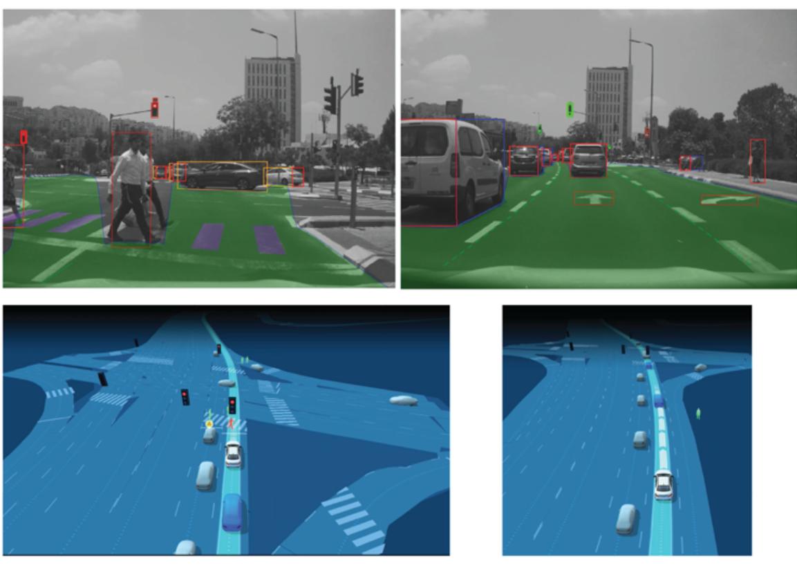
Mobileye’s camera-based sensing for autonomous vehicles. Top row: Two images from a front-facing camera, taken a few seconds apart. The green area is the free space—the area to which the vehicle could physically move in the immediate future. Objects are displayed with 3D bounding boxes defining their sides (red for the rear, blue for the right side, yellow for the left side, and green for the front). Objects include vehicles, pedestrians, the inner edge of the self-lane marks (necessary for lateral control), other painted road and crosswalk marks, traffic signs, and traffic lights. Not shown are animals, poles and cones, sidewalks, railings, and general objects (e.g., a couch that fell from the back of a truck). Each object is then marked with a 3D position and velocity. Bottom row: A full physical model of the environment, rendered from the detected objects.

(Images show Mobileye’s vision-only system results). Images courtesy of Mobileye.

Roads were designed for humans who navigate using vision, so it should in principle be possible to drive using vision alone. However, in practice, commercial self-driving cars use a variety of sensors, including cameras, lidars, radars, and microphones. A lidar or radar

enables direct measurement of depth, which can be more accurate than the vision-only methods of Section 25.6 . Having multiple sensors increases performance in general, and is particularly important in conditions of poor visibility; for example, radar can cut through fog that blocks cameras and lidars. Microphones can detect approaching vehicles (especially ones with sirens) before they become visible.

There has also been much research on mobile robots navigating in indoor and outdoor environments. Applications abound, such as the last mile of package or pizza delivery. Traditional approaches break this task up into two stages as shown in Figure 25.29 :

• MAP BUILDING: Simultaneous Localization and Mapping or SLAM (see page 935) is the task of constructing a 3D model of the world, including the location of the robot in the world (or more specifically, the location of each of the robot’s cameras). This model (typically represented as a point cloud of obstacles) can be built from a series of images from different camera positions.
• PATH PLANNING: Once the robot has access to this 3D map and can localize itself in it, the objective becomes one of finding a collision-free trajectory from the current position to the goal location (see Section 26.6 ).

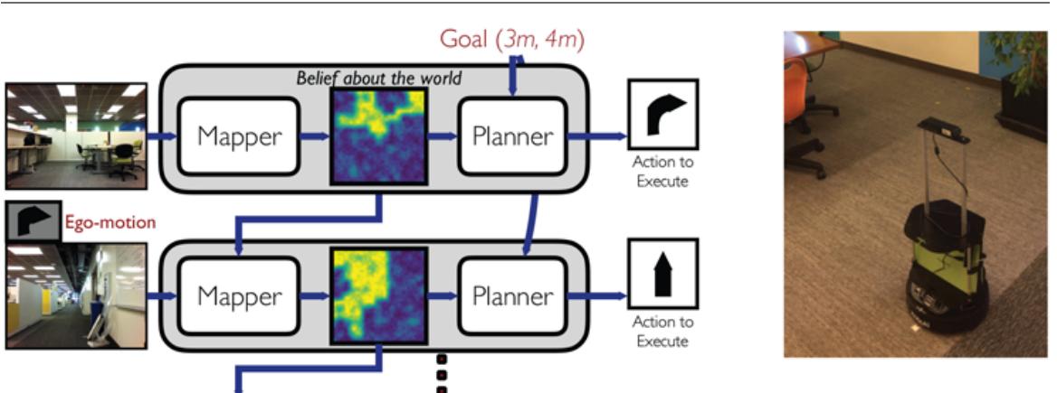
Figure 25.29

Navigation is tackled by decomposition into two problems: mapping and planning. With each successive time step, information from sensors is used to incrementally build an uncertain model of the world. This model along with the goal specification is passed to a planner that outputs the next action that the robot should take in order to achieve the goal. Models of the world can be purely geometric (as in classical SLAM), or semantic (as obtained via learning), or even topological (based on landmarks). The actual robot appears on the right.

Figures courtesy of Saurabh Gupta.

Many variants of this general approach have been explored. For instance, in the cognitive mapping and planning approach, the two stages of map building and path planning are two modules in a neural network that is trained end-to-end to minimize a loss function. Such a system does not have to build a complete map—which is often redundant and unnecessary if all you need is enough information to navigate from point A to point B without colliding with obstacles.

Summary

Although perception appears to be an effortless activity for humans, it requires a significant amount of sophisticated computation. The goal of vision is to extract information needed for tasks such as manipulation, navigation, and object recognition.

• The geometry and optics of image formation is well understood. Given a description of a 3D scene, we can easily produce a picture of it from some arbitrary camera position this is the graphics problem. The inverse problem, the computer vision problem—taking a picture and turning it into a 3D description—is more difficult.
• Representations of images capture edges, texture, optical flow, and regions. These yield cues to the boundaries of objects and to correspondence between images.
• Convolutional neural networks produce accurate image classifiers that use learned features. Rather roughly, the features are patterns of patterns of patterns. . . . It is hard to predict when these classifiers will work well, because the test data may be unlike the training data in some important way. Experience teaches that they are often accurate enough to use in practice.
• Image classifiers can be turned into object detectors. One classifier scores boxes in an image for objectness; another then decides whether an object is in the box, and what object it is. Object detection methods aren’t perfect, but are usable for a wide variety of applications.
• With more than one view of a scene, it is possible to recover the 3D structure of the scene and the relationship between views. In many cases, it is possible to recover 3D geometry from a single view.
• The methods of computer vision are being very widely applied.

Bibliographical and Historical Notes

This chapter has concentrated on vision, but other perceptual channels have been studied and put to use in robotics. For auditory perception (hearing), we have already covered speech recognition, and there has also been considerable work on music perception (Koelsch and Siebel, 2005) and machine learning of music (Engel et al., 2017) as well as on machine learning for sounds in general (Sharan and Moir, 2016).

Tactile perception or touch (Luo et al., 2017) is important in robotics and is discussed in Chapter 26 . Automated olfactory perception (smell) has seen less work, but it has been shown that deep learning models can learn to predict smells based on the structure of molecules (Sanchez-Lengeling et al., 2019).

Systematic attempts to understand human vision can be traced back to ancient times. Euclid (ca. 300 BCE) wrote about natural perspective—the mapping that associates, with each point in the three-dimensional world, the direction of the ray joining the center of projection to the point . He was well aware of the notion of motion parallax. Ancient Roman paintings, such as the ones perserved by the eruption of Vesuvius in 79 CE, used an informal kind of perspective, with more than one horizon line.

The mathematical understanding of perspective projection, this time in the context of projection onto planar surfaces, had its next significant advance in the 15th century in Renaissance Italy. Brunelleschi is usually credited with creating the first paintings based on geometrically correct projection of a three-dimensional scene in about 1413. In 1435, Alberti codified the rules and inspired generations of artists. Particularly notable in their development of the science of perspective, as it was called in those days, were Leonardo da Vinci and Albrecht Dürer. Leonardo’s late 15th-century descriptions of the interplay of light and shade (chiaroscuro), umbra and penumbra regions of shadows, and aerial perspective are still worth reading in translation (Kemp, 1989).

Although perspective was known to the Greeks, they were curiously confused by the role of the eyes in vision. Aristotle thought of the eyes as devices emitting rays, rather in the manner of modern laser range finders. This mistaken view was laid to rest by the work of Arab scientists, such as Alhazen, in the 10th century.

The development of various kinds of cameras followed. These consisted of rooms (camera is Latin for “chamber”) where light would be let in through a small hole in one wall to cast an image of the scene outside on the opposite wall. Of course, in all these cameras, the image was inverted, which caused no end of confusion. If the eye was to be thought of as such an imaging device, how do we see right side up? This enigma exercised the greatest minds of the era (including Leonardo). It took the work of Kepler and Descartes to settle the question. Descartes placed an eye from which the opaque cuticle had been removed in a hole in a window shutter. The result was an inverted image formed on a piece of paper laid out on the retina. Although the retinal image is indeed inverted, this does not cause a problem because the brain interprets the image the right way. In modern jargon, one just has to access the data structure appropriately.

The next major advances in the understanding of vision took place in the 19th century. The work of Helmholtz and Wundt, described in Chapter 1 , established psychophysical experimentation as a rigorous scientific discipline. Through the work of Young, Maxwell, and Helmholtz, a trichromatic theory of color vision was established. The fact that humans can see depth if the images presented to the left and right eyes are slightly different was demonstrated by Wheatstone’s (1838) invention of the stereoscope. The device immediately became popular in parlors and salons throughout Europe.

The essential concept of binocular stereopsis—that two images of a scene taken from slightly different viewpoints carry information sufficient to obtain a three-dimensional reconstruction of the scene—was exploited in the field of photogrammetry. Key mathematical results were obtained; for example, Kruppa (1913) proved that, given two views of five distinct points in a scene, one could reconstruct the rotation and translation between the two camera positions as well as the depth of the scene (up to a scale factor).

Although the geometry of stereopsis had been understood for a long time, the correspondence problem in photogrammetry used to be solved by humans trying to match up corresponding points. The amazing ability of humans in solving the correspondence problem was illustrated by Julesz’s (1971) random dot stereograms. The field of computer vision has devoted much effort towards an automatic solution of the correspondence problem.

In the first half of the 20th century, the most significant research results in vision were obtained by the Gestalt school of psychology, led by Max Wertheimer. They pointed out the importance of perceptual organization: for a human, the image is not a collection of pointillist photoreceptor outputs (pixels), rather it is organized into coherent groups. The computer vision task of finding regions and curves traces back to this insight. The Gestaltists also drew attention to the “figure-ground” phenomenon—a contour separating two image regions that in the world are at different depths appears to belong only to the nearer region, the “figure,” and not to the farther region, the “ground.”

The gestalt work was carried on by J. J. Gibson (1950, 1979), who pointed out the importance of optical flow and texture gradients in the estimation of environmental variables such as surface slant and tilt. He reemphasized the importance of the stimulus and how rich it was. Gibson, Olum, and Rosenblatt (1955) pointed out that the optical flow field contained enough information to determine the motion of the observer relative to the environment. Gibson particularly emphasized the role of the active observer, whose selfdirected movement facilitates the pickup of information about the external environment.

Computer vision dates back to the 1960s. Roberts’s (1963) thesis at MIT on perceiving cubes and other blocks-world objects was one of the earliest publications in the field. Roberts introduced several key ideas, including edge detection and model-based matching.

In the 1960s and 1970s progress was slow, hampered by the lack of computational and storage resources. Low-level visual processing received a lot of attention, with techniques drawn from related fields such as signal processing, pattern recognition, and data clustering.

Edge detection was treated as an essential first step in image processing, as it reduced the amount of data to be processed. The widely used Canny edge detection technique was introduced by John Canny (1986). Martin, Fowlkes, and Malik (2004) showed how to combine multiple clues, such as brightness, texture and color, in a machine learning framework to better find boundary curves.

The closely related problem of finding regions of coherent brightness, color, and texture naturally lends itself to formulations where finding the best partition becomes an optimization problem. Three leading examples are based on Markov Random Fields due to Geman and Geman (1984), the variational formulation of Mumford and Shah (1989), and normalized cuts by Shi and Malik (2000).

Through much of the 1960s, 1970s, and 1980s, there were two distinct paradigms in which visual recognition was pursued, dictated by different perspectives on what was perceived to be the primary problem. Computer vision research on object recognition largely focused on issues arising from the projection of three-dimensional objects onto two-dimensional images. The idea of alignment, also first introduced by Roberts, resurfaced in the 1980s in the work of Lowe (1987) and Huttenlocher and Ullman (1990).

The pattern recognition community took a different approach, viewing the 3D–to–2D aspects of the problem as insignificant. Their motivating examples were in domains such as optical character recognition and handwritten zip code recognition, in which the primary concern is that of learning the typical variations characteristic of a class of objects and separating them from other classes. We can trace neural net architectures for image analysis back to Hubel and Wiesel’s (1962, 1968) studies of the visual cortex in cats and monkeys. They developed a hierarchical model of the visual pathway with neurons in lower areas of the brain (especially the area called V1) responding to features such as oriented edges and bars, and neurons in higher areas responding to more specific stimuli (“grandmother cells” in the cartoon version).

Fukushima (1980) proposed a neural network architecture for pattern recognition explicitly motivated by Hubel and Wiesel’s hierarchy. His model had alternating layers of simple cells and complex cells, thus incorporating downsampling, and also had shift invariance, thus incorporating convolutional structure. LeCun et al. (1989) took the additional step of using back-propagation to train the weights of this network, and what we today call convolutional neural networks were born. See LeCun et al. (1995) for a comparison of approaches.

Starting in the late 1990s, accompanying a much greater role of probabilistic modeling and statistical machine learning in the field of artificial intelligence in general, there was a rapprochement between these two traditions. Two lines of work contributed significantly. One was research on face detection (Rowley et al., 1998; Viola and Jones, 2004) that demonstrated the power of pattern recognition techniques on clearly important and useful tasks.

The other was the development of point descriptors, which enable the construction of feature vectors from parts of objects (Schmid and Mohr, 1996). There are three key strategies to build a good local point descriptor: one uses orientations to get illumination invariance; one needs to describe image structure close to a point in detail, and further away only roughly; and one needs to use spatial histograms to suppress variations caused by small errors in locating the point. Lowe’s (2004) SIFT descriptor exploited these ideas very effectively; another popular variant was the HOG descriptor due to Dalal and Triggs (2005).

The 1990s and 2000s saw a continuing debate between the devotees of clever feature design such as SIFT and HOG and the aficionados of neural networks who believed that good features should emerge automatically from end-to-end training. The way to settle such a debate is through benchmarks on standard data sets, and in the 2000s results on a standard object detection data set, PASCAL VOC, argued in favor of hand-designed features. This changed when Krizhevsky et al. (2013) showed that on the task of image classification on the ImageNet data set, their neural network (called AlexNet) gave significantly lower error rates than the mainstream computer vision techniques.

What was the secret sauce behind the success of AlexNet? Besides the technical innovations (such as the use of ReLU activation units) we must give a lot of credit to big data and big computation. By big data we mean the availability of large data sets with category labels, such as ImageNet, which provided the training data for these large, deep networks with millions of parameters. Previous data sets like Caltech-101 or PASCAL VOC didn’t have enough training data, and MNIST and CIFAR were regarded as “toy data sets” by the computer vision community. This strand of labeling data sets for benchmarking and for extracting image statistics itself was enabled by the desire of people to upload their photo collections to the Internet on sites such as Flickr. The way big computation proved most helpful was through GPUs, a hardware development initially driven by the needs of the video game industry.

Within a year or two, the evidence was quite clear. For example, the region-based convolutional neural network (RCNN) work of Girshick et al. (2016) showed that the AlexNet architecture could be modified, by making use of computer vision ideas such as region proposals, to make possible state-of-the-art object detection on PASCAL VOC.We have realized that generally deeper networks work better and that overfitting fears are

overblown. We have new techniques such as batch normalization to deal with regularization.

The reconstruction of three-dimensional structure from multiple views has its roots in the photogrammetry literature. In the computer vision era, Ullman (1979), and Longuet-Higgins (1981) are influential early works. Concerns about the stability of structure from motion were significantly allayed by the work of Tomasi and Kanade (1992) who showed that with the use of multiple frames, and the resulting wide baseline, shape could be recovered quite accurately.

A conceptual innovation introduced in the 1990s was the study of projective structure from motion. Here camera calibration is not necessary, as was shown by Faugeras (1992). This discovery is related to the introduction of the use of geometrical invariants in object recognition, as surveyed by Mundy and Zisserman (1992), and the development of affine structure from motion by Koenderink and Van Doorn (1991).

In the 1990s, with great increase in computer speed and storage and the widespread availability of digital video, motion analysis found many new applications. Building geometrical models of real-world scenes for rendering by computer graphics techniques proved particularly popular, led by reconstruction algorithms such as the one developed by Debevec et al. (1996). The books by Hartley and Zisserman (2000) and Faugeras et al. (2001) provide a comprehensive treatment of the geometry of multiple views.

Humans can perceive shape and spatial layout from a single image, and modeling this has proved to be quite a challenge for computer vision researchers. Inferring shape from shading was first studied by Berthold Horn (1970), and Horn and Brooks (1989) present an extensive survey of the main papers from a period when this was a much studied problem. Gibson (1950) was the first to propose texture gradients as a cue to shape. The mathematics of occluding contours, and more generally understanding the visual events in the projection of smooth curved objects, owes much to the work of Koenderink and van Doorn, which finds an extensive treatment in Koenderink’s (1990) Solid Shape.

More recently, attention has turned to treating the problem of shape and surface recovery from a single image as a probabilistic inference problem, where geometrical cues are not

modeled explicitly, but used implicitly in a learning framework. A good example is the work of Hoiem et al. (2007); recently this has been reworked using deep neural networks.

Turning now to the applications of computer vision for guiding action, Dickmanns and Zapp (1987) first demonstrated a self-driving car driving on freeways at high speeds; Pomerleau (1993) achieved similar performance using a neural network approach. Today building selfdriving cars is a big business, with the established car companies competing with new entrants such as Baidu, Cruise, Didi, Google Waymo, Lyft, Mobileye, Nuro, Nvidia, Samsung, Tata, Tesla, Uber, and Voyage to market systems that provide capabilities ranging from driver assistance to full autonomy.

For the reader interested in human vision, Vision Science: Photons to Phenomenology by Stephen Palmer (1999) provides the best comprehensive treatment; Visual Perception: Physiology, Psychology and Ecology by Vicki Bruce, Patrick Green, and Mark Georgeson (2003) is a shorter textbook. The books Eye, Brain and Vision by David Hubel (1988) and Perception by Irvin Rock (1984) are friendly introductions centered on neurophysiology and perception respectively. David Marr’s book Vision (Marr, 1982) played a historical role in connecting computer vision to the traditional areas of biological vision—psychophysics and neurobiology. While many of his specific models for tasks such as edge detection and object recognition haven’t stood the test of time, the theoretical perspective where each task is analyzed at an informational, computational, and implementation level is still illuminating.

For the field of computer vision, the most comprehensive textbooks available today are Computer Vision: A Modern Approach (Forsyth and Ponce, 2002) and Computer Vision: Algorithms and Applications (Szeliski, 2011). Geometrical problems in computer vision are treated thoroughly in Multiple View Geometry in Computer Vision (Hartley and Zisserman, 2000). These books were written before the deep learning revolution, so for the latest results, consult the primary literature.

Two of the main journals for computer vision are the IEEE Transactions on Pattern Analysis and Machine Intelligence and the International Journal of Computer Vision. Computer vision conferences include ICCV (International Conference on Computer Vision), CVPR (Computer Vision and Pattern Recognition), and ECCV (European Conference on Computer Vision). Research with a significant machine learning component is also published at NeurIPS (Neural Information Processing Systems), and work on the interface with computer

graphics often appears at the ACM SIGGRAPH (Special Interest Group in Graphics) conference. Many vision papers appear as preprints on the arXiv server, and early reports of new results appear in blogs from the major research labs.

Chapter 26 Robotics

In which agents are endowed with sensors and physical effectors with which to move about and make mischief in the real world.

26.1 Robots

Robots are physical agents that perform tasks by manipulating the physical world. To do so, they are equipped with effectors such as legs, wheels, joints, and grippers. Effectors are designed to assert physical forces on the environment. When they do this, a few things may happen: the robot’s state might change (e.g., a car spins its wheels and makes progress on the road as a result), the state of the environment might change (e.g., a robot arm uses its gripper to push a mug across the counter), and even the state of the people around the robot might change (e.g., an exoskeleton moves and that changes the configuration of a person’s leg; or a mobile robot makes progress toward the elevator doors, and a person notices and is nice enough to move out of the way, or even push the button for the robot).

Robot

Effector

Robots are also equipped with sensors, which enable them to perceive their environment. Present-day robotics employs a diverse set of sensors, including cameras, radars, lasers, and microphones to measure the state of the environment and of the people around it; and gyroscopes, strain and torque sensors, and accelerometers to measure the robot’s own state.

Sensor

Maximizing expected utility for a robot means choosing how to actuate its effectors to assert the right physical forces—the ones that will lead to changes in state that accumulate as much

expected reward as possible. Ultimately, robots are trying to accomplish some task in the physical world.

Robots operate in environments that are partially observable and stochastic: cameras cannot see around corners, and gears can slip. Moreover, the people acting in that same environment are unpredictable, so the robot needs to make predictions about them.

Robots usually model their environment with a continuous state space (the robot’s position has continuous coordinates) and a continuous action space (the amount of current a robot sends to its motor is also measured in continuous units). Some robots operate in highdimensional spaces: cars need to know the position, orientation, and velocity of themselves and the nearby agents; robot arms have six or seven joints that can each be independently moved; and robots that mimic the human body have hundreds of joints.

Robotic learning is constrained because the real world stubbornly refuses to operate faster than real time. In a simulated environment, it is possible to use learning algorithms (such as the Q-learning algorithm described in Chapter 22 ) to learn in a few hours from millions of trials. In a real environment, it might take years to run these trials, and the robot cannot risk (and thus cannot learn from) a trial that might cause harm. Thus, transferring what has been learned in simulation to a real robot in the real world—the sim-to-real problem—is an active area of research. Practical robotic systems need to embody prior knowledge about the robot, the physical environment, and the tasks to be performed so that the robot can learn quickly and perform safely.

Robotics brings together many of the concepts we have seen in this book, including probabilistic state estimation, perception, planning, unsupervised learning, reinforcement learning, and game theory. For some of these concepts robotics serves as a challenging example application. For other concepts this chapter breaks new ground, for instance in introducing the continuous version of techniques that we previously saw only in the discrete case.

26.2 Robot Hardware

So far in this book, we have taken the agent architecture—sensors, effectors, and processors —as given, and have concentrated on the agent program. But the success of real robots depends at least as much on the design of sensors and effectors that are appropriate for the task.

26.2 Types of robots from the hardware perspective

When you think of a robot, you might imagine something with a head and two arms, moving around on legs or wheels. Such anthropomorphic robots have been popularized in fiction such as the movie The Terminator and the cartoon The Jetsons. But real robots come in many shapes and sizes.

Anthropomorphic robot

Manipulator

Manipulators are just robot arms. They do not necessarily have to be attached to a robot body; they might simply be bolted onto a table or a floor, as they are in factories (Figure 26.1 (a) ). Some have a large payload, like those assembling cars, while others, like wheelchair-mountable arms that assist people with motor impairments (Figure 26.1 (b) ), can carry less but are safer in human environments.

Figure 26.1

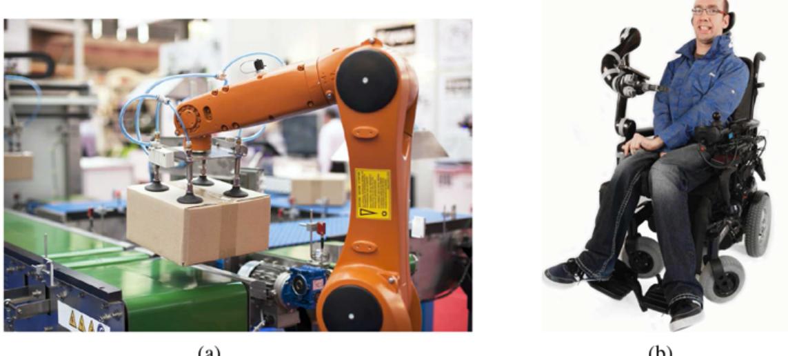
1. An industrial robotic arm with a custom end-effector. Image credit: Macor/123RF. (b) A Kinova JACO Assistive Robot arm mounted on a wheelchair. Kinova and JACO are trademarks of Kinova, Inc. ® ®

Mobile robots are those that use wheels, legs, or rotors to move about the environment. Quadcopter drones are a type of unmanned aerial vehicle (UAV); autonomous underwater vehicles (AUVs) roam the oceans. But many mobile robots stay indoors and move on wheels, like a vacuum cleaner or a towel delivery robot in a hotel. Their outdoor counterparts include autonomous cars or rovers that explore new terrain, even on the surface of Mars (Figure 26.2 ). Finally, legged robots are meant to traverse rough terrain that is inaccessible with wheels. The downside is that controlling legs to do the right thing is more challenging than spinning wheels.

Figure 26.2

1. NASA’s Curiosity rover taking a selfie on Mars. Image courtesy of NASA. (b) A Skydio drone accompanying a family on a bike ride. Image courtesy of Skydio.

Mobile robot

Quadcopter drone

UAV

AUV

Autonomous car

Rover

Legged robot

Other kinds of robots include prostheses, exoskeletons, robots with wings, swarms, and intelligent environments in which the robot is the entire room.

26.2.2 Sensing the world

Sensors are the perceptual interface between robot and environment. Passive sensors, such as cameras, are true observers of the environment: they capture signals that are generated by other sources in the environment. Active sensors, such as sonar, send energy into the environment. They rely on the fact that this energy is reflected back to the sensor. Active sensors tend to provide more information than passive sensors, but at the expense of increased power consumption and with a danger of interference when multiple active sensors are used at the same time. We also distinguish whether a sensor is directed at sensing the environment, the robot’s location, or the robot’s internal configuration.

Passive sensor

Active sensor

Range finder

Sonar

Stereo vision

Range finders are sensors that measure the distance to nearby objects. Sonar sensors are active range finders that emit directional sound waves, which are reflected by objects, with some of the sound making it back to the sensor. The time and intensity of the returning signal indicates the distance to nearby objects. Sonar is the technology of choice for autonomous underwater vehicles, and was popular in the early days of indoor robotics. Stereo vision (see Section 25.6 ) relies on multiple cameras to image the environment from slightly different viewpoints, analyzing the resulting parallax in these images to compute the range of surrounding objects.

For mobile ground robots, sonar and stereo vision are now rarely used, because they are not reliably accurate. The Kinect is a popular low-cost sensor that combines a camera and a structured light projector, which projects a pattern of grid lines onto a scene. The camera sees how the grid lines bend, giving the robot information about the shape of the objects in the scene. If desired, the projection can be infrared light, so as not to interfere with other sensors (such as human eyes).

Structured light

Most ground robots are now equipped with active optical range finders. Just like sonar sensors, optical range sensors emit active signals (light) and measure the time until a reflection of this signal arrives back at the sensor. Figure 26.3(a) shows a time-of-flight camera. This camera acquires range images like the one shown in Figure 26.3(b) at up to 60 frames per second. Autonomous cars often use scanning lidars (short for light detection and ranging)—active sensors that emit laser beams and sense the reflected beam, giving

range measurements accurate to within a centimeter at a range of 100 meters. They use complex arrangements of mirrors or rotating elements to sweep the beam across the environment and build a map. Scanning lidars tend to work better than time-of-flight cameras at longer ranges, and tend to perform better in bright daylight.

1. Time-of-flight camera; image courtesy of Mesa Imaging GmbH. (b) 3D range image obtained with this camera. The range image makes it possible to detect obstacles and objects in a robot’s vicinity. Image courtesy of Willow Garage, LLC.

Time-of-fligh camera

Figure 26.3

Scanning lidar

Radar is often the range finding sensor of choice for air vehicles (autonomous or not). Radar sensors can measure distances up to kilometers, and have an advantage over optical sensors in that they can see through fog. On the close end of range sensing are tactile sensors such

as whiskers, bump panels, and touch-sensitive skin. These sensors measure range based on physical contact, and can be deployed only for sensing objects very close to the robot.

Radar Tactile sensor Location sensor

Global Positioning System

A second important class is location sensors. Most location sensors use range sensing as a primary component to determine location. Outdoors, the Global Positioning System (GPS) is the most common solution to the localization problem. GPS measures the distance to satellites that emit pulsed signals. At present, there are 31 operational GPS satellites in orbit, and 24 GLONASS satellites, the Russian counterpart. GPS receivers can recover the distance to a satellite by analyzing phase shifts. By triangulating signals from multiple satellites, GPS receivers can determine their absolute location on Earth to within a few meters. Differential GPS involves a second ground receiver with known location, providing millimeter accuracy under ideal conditions.

Differential GPS

Unfortunately, GPS does not work indoors or underwater. Indoors, localization is often achieved by attaching beacons in the environment at known locations. Many indoor environments are full of wireless base stations, which can help robots localize through the analysis of the wireless signal. Underwater, active sonar beacons can provide a sense of location, using sound to inform AUVs of their relative distances to those beacons.

The third important class is proprioceptive sensors, which inform the robot of its own motion. To measure the exact configuration of a robotic joint, motors are often equipped with shaft decoders that accurately measure the angular motion of a shaft. On robot arms, shaft decoders help track the position of joints. On mobile robots, shaft decoders report wheel revolutions for odometry—the measurement of distance traveled. Unfortunately, wheels tend to drift and slip, so odometry is accurate only over short distances. External forces, such as wind and ocean currents, increase positional uncertainty. Inertial sensors, such as gyroscopes, reduce uncertainty by relying on the resistance of mass to the change of velocity.

Proprioceptive sensor

Shaft decoder

Odometry

Inertial sensor

Other important aspects of robot state are measured by force sensors and torque sensors. These are indispensable when robots handle fragile objects or objects whose exact size and shape are unknown. Imagine a one-ton robotic manipulator screwing in a light bulb. It would be all too easy to apply too much force and break the bulb. Force sensors allow the robot to sense how hard it is gripping the bulb, and torque sensors allow it to sense how hard it is turning. High-quality sensors can measure forces in all three translational and three rotational directions. They do this at a frequency of several hundred times a second so that a robot can quickly detect unexpected forces and correct its actions before it breaks a light bulb. However, it can be a challenge to outfit a robot with high-end sensors and the computational power to monitor them.

Force sensor

Torque sensor

26.2.3 Producing motion

The mechanism that initiates the motion of an effector is called an actuator; examples include transmissions, gears, cables, and linkages. The most common type of actuator is the electric actuator, which uses electricity to spin up a motor. These are predominantly used in systems that need rotational motion, like joints on a robot arm. Hydraulic actuators use pressurized hydraulic fluid (like oil or water) and pneumatic actuators use compressed air to generate mechanical motion.

Actuator

Hydraulic actuator

Pneumatic actuator

Actuators are often used to move joints, which connect rigid bodies (links). Arms and legs have such joints. In revolute joints, one link rotates with respect to the other. In prismatic joints, one link slides along the other. Both of these are single-axis joints (one axis of motion). Other kinds of joints include spherical, cylindrical, and planar joints, which are multi-axis joints.

Revolute joint

Prismatic joint

Parallel jaw gripper

To interact with objects in the environment, robots use grippers. The most basic type of gripper is the parallel jaw gripper, with two fingers and a single actuator that moves the fingers together to grasp objects. This effector is both loved and hated for its simplicity. Three-fingered grippers offer slightly more flexibility while maintaining simplicity. At the other end of the spectrum are humanoid (anthropomorphic) hands. For instance, the Shadow Dexterous Hand has a total of 20 actuators. This offers a lot more flexibility for complex manipulation, including in-hand manipulator maneuvers (think of picking up your cell phone and rotating it in-hand to orient it right-side up), but this flexibility comes at a price—learning to control these complex grippers is more challenging.

26.3 What kind of problem is robotics solving?

Now that we know what the robot hardware might be, we’re ready to consider the agent software that drives the hardware to achieve our goals. We first need to decide the computational framework for this agent. We have talked about search in deterministic environments, MDPs for stochastic but fully observable environments, POMDPs for partial observability, and games for situations in which the agent is not acting in isolation. Given a computational framework, we need to instantiate its ingredients: reward or utility functions, states, actions, observation spaces, etc.

We have already noted that robotics problems are nondeterministic, partially observable, and multiagent. Using the game-theoretic notions from Chapter 18 , we can see that sometimes the agents are cooperative and sometimes they are competitive. In a narrow corridor where only one agent can go first, a robot and a person collaborate because they both want to make sure they don’t bump into each other. But in some cases they might compete a bit to reach their destination quickly. If the robot is too polite and always makes room, it might get stuck in crowded situations and never reach its goal.

Therefore, when robots act in isolation and know their environment, the problem they are solving can be formulated as an MDP; when they are missing information it becomes a POMDP; and when they act around people it can often be formulated as a game.

What is the robot’s reward function in this formulation? Usually the robot is acting in service of a human—for example delivering a meal to a hospital patient for the patient’s reward, not its own. For most robotics settings, even though robot designers might try to specify a good enough proxy reward function, the true reward function lies with the user whom the robot is supposed to help. The robot will either need to decipher the user’s desires, or rely on an engineer to specify an approximation of the user’s desires.

As for the robot’s action, state, and observation spaces, the most general form is that observations are raw sensor feeds (e.g., the images coming in from cameras, or the laser hits coming in from lidar); actions are raw electric currents being sent to the motors; and state is what the robot needs to know for its decision making. This means there is a huge gap

between the low-level percepts and motor controls, and the high-level plans the robot needs to make. To bridge the gap, roboticists decouple aspects of the problem to simplify it.

For instance, we know that when we solve POMDPs properly, perception and action interact: perception informs which actions make sense, but action also informs perception, with agents taking actions to gather information when that information has value in later time steps. However, robots often separate perception from action, consuming the outputs of perception and pretending they will not get any more information in the future. Further, hierarchical planning is called for, because a high-level goal like “get to the cafeteria” is far removed from a motor command like “rotate the main axle”

In robotics we often use a three-level hierarchy. The task planning level decides a plan or policy for high-level actions, sometimes called action primitives or subgoals: move to the door, open it, go to the elevator, press the button, etc. Then motion planning is in charge of finding a path that gets the robot from one point to another, achieving each subgoal. Finally, control is used to achieve the planned motion using the robot’s actuators. Since the task planning level is typically defined over discrete states and actions, in this chapter we will focus primarily on motion planning and control.

Task planning

Control

Separately, preference learning is in charge of estimating an end user’s objective, and people prediction is used to forecast the actions of other people in the robot’s environment. All these combine to determine the robot’s behavior.

Preference learning

People prediction

Whenever we split a problem into separate pieces we reduce complexity, but we give up opportunities for the pieces to help each other. Action can help improve perception, and also determine what kind of perception is useful. Similarly, decisions at the motion level might not be the best when accounting for how that motion will be tracked; or decisions at the task level might render the task plan uninstantiatable at the motion level. So, with progress in these separate areas comes the push to reintegrate them: to do motion planning and control together, to do task and motion planning together, and to reintegrate perception, prediction, and action—closing the feedback loop. Robotics today is about continuing progress in each area while also building on this progress to achieve better integration.

26.4 Robotic Perception

Perception is the process by which robots map sensor measurements into internal representations of the environment. Much of it uses the computer vision techniques from the previous chapter. But perception for robotics must deal with additional sensors like lidar and tactile sensors.

Perception is difficult because sensors are noisy and the environment is partially observable, unpredictable, and often dynamic. In other words, robots have all the problems of state estimation (or filtering) that we discussed in Section 14.2 . As a rule of thumb, good internal representations for robots have three properties:

• 1. They contain enough information for the robot to make good decisions.
• 2. They are structured so that they can be updated efficiently.
• 3. They are natural in the sense that internal variables correspond to natural state variables in the physical world.

In Chapter 14 , we saw that Kalman filters, HMMs, and dynamic Bayes nets can represent the transition and sensor models of a partially observable environment, and we described both exact and approximate algorithms for updating the belief state—the posterior probability distribution over the environment state variables. Several dynamic Bayes net models for this process were shown in Chapter 14 . For robotics problems, we include the robot’s own past actions as observed variables in the model. Figure 26.4 shows the notation used in this chapter: is the state of the environment (including the robot) at time is the observation received at time and is the action taken after the observation is received.

Figure 26.4

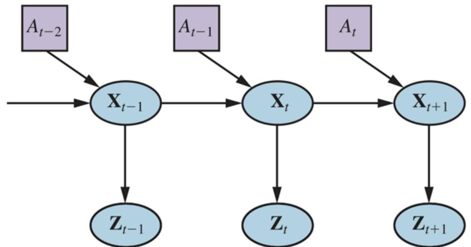
Robot perception can be viewed as temporal inference from sequences of actions and measurements, as illustrated by this dynamic decision network.

We would like to compute the new belief state, from the current belief state, and the new observation We did this in Section 14.2 , but there are two differences here: we condition on the actions as well as the observations, and we deal with continuous rather than discrete variables. Thus, we modify the recursive filtering equation (14.5 on page 467) to use integration rather than summation:

(26.1)

\[\begin{aligned} &\mathbf{P}\left(\mathbf{X}\_{t+1}|\mathbf{z}\_{1:t+1},a\_{1:t}\right) \\ &= \alpha \mathbf{P}\left(\mathbf{z}\_{t+1}|\mathbf{X}\_{t+1}\right) \int \mathbf{P}\left(\mathbf{X}\_{t+1}|\mathbf{x}\_{t},a\_{t}\right) P\left(\mathbf{x}\_{t}|\mathbf{z}\_{1:t},a\_{1:t-1}\right) \,d\mathbf{x}\_{t} .\end{aligned}\]

This equation states that the posterior over the state variables at time is calculated recursively from the corresponding estimate one time step earlier. This calculation involves the previous action and the current sensor measurement For example, if our goal is to develop a soccer-playing robot, might include the location of the soccer ball relative to the robot. The posterior is a probability distribution over all states that captures what we know from past sensor measurements and controls. Equation (26.1) tells us how to recursively estimate this location, by incrementally folding in sensor measurements (e.g., camera images) and robot motion commands. The probability is called the transition model or motion model, and is the sensor model.

26.4.1 Localization and mapping

Localization is the problem of finding out where things are—including the robot itself. To keep things simple, let us consider a mobile robot that moves slowly in a flat twodimensional world. Let us also assume the robot is given an exact map of the environment. (An example of such a map appears in Figure 26.7 .) The pose of such a mobile robot is defined by its two Cartesian coordinates with values and and its heading with value as illustrated in Figure 26.5 (a) . If we arrange those three values in a vector, then any particular state is given by So far so good.

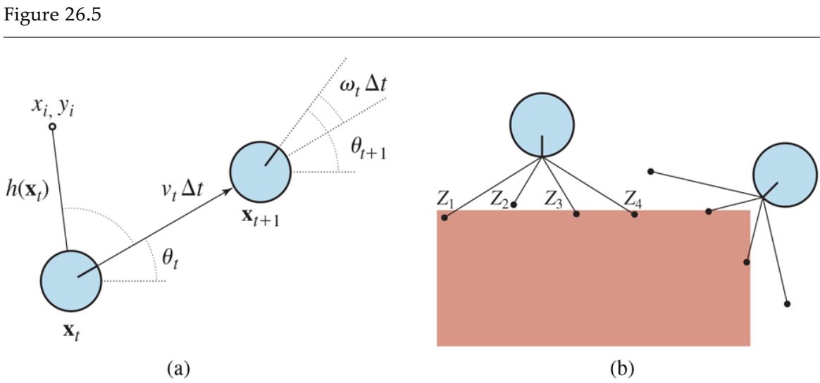
1. A simplified kinematic model of a mobile robot. The robot is shown as a circle with an interior radius line marking the forward direction. The state consists of the position (shown implicitly) and the orientation The new state is obtained by an update in position of and in orientation of Also shown is a landmark at observed at time (b) The range-scan sensor model. Two possible robot poses are shown for a given range scan It is much more likely that the pose on the left generated the range scan than the pose on the right.

Localization

In the kinematic approximation, each action consists of the “instantaneous” specification of two velocities—a translational velocity and a rotational velocity For small time intervals a crude deterministic model of the motion of such robots is given by

\[\hat{\mathbf{X}}\_{t+1+} = f(\mathbf{X}\_{t, \underbrace{v\_t, \omega\_t}\_{a\_t})} = \mathbf{X}\_t + \begin{pmatrix} v\_t \triangle t \cos \theta\_t \\ v\_t \triangle t \sin \theta\_t \\ \omega\_t \triangle t \end{pmatrix}.\]

The notation refers to a deterministic state prediction. Of course, physical robots are somewhat unpredictable. This is commonly modeled by a Gaussian distribution with mean and covariance (See Appendix A for a mathematical definition.)

\[\mathbf{P}(\mathbf{X}\_{t+1} \mid \mathbf{X}\_t, v\_t, \omega\_t) = N(\mathbf{X}\_{t+1}, \Sigma\_x).\]

This probability distribution is the robot’s motion model. It models the effects of the motion on the location of the robot.

Next, we need a sensor model. We will consider two kinds of sensor models. The first assumes that the sensors detect stable, recognizable features of the environment called landmarks. For each landmark, the range and bearing are reported. Suppose the robot’s state is and it senses a landmark whose location is known to be Without noise, a prediction of the range and bearing can be calculated by simple geometry (see Figure 26.5 (a) ):

\[\hat{\mathbf{z}}\_{t} = h(\mathbf{x}\_{t}) = \left( \sqrt{\frac{\left(x\_{t} - x\_{i}\right)^{2} + \left(y\_{t} - y\_{i}\right)^{2}}{x\_{t} - y\_{t}}} \right).\]

\[\left(\arctan\frac{y\_{i} - y\_{t}}{x\_{i} - x\_{t}} - \theta\_{t}\right).\]

Landmark

Again, noise distorts our measurements. To keep things simple, assume Gaussian noise with covariance giving us the sensor model

\[P(\mathbf{z}\_t|\mathbf{x}\_t) = N(\hat{\mathbf{z}}\_t, \Sigma\_z).\]

A somewhat different sensor model is used for a sensor array of range sensors, each of which has a fixed bearing relative to the robot. Such sensors produce a vector of range values

Sensor array

Given a pose let be the computed range along the th beam direction from to the nearest obstacle. As before, this will be corrupted by Gaussian noise. Typically, we assume that the errors for the different beam directions are independent and identically distributed, so we have

\[P(\mathbf{z}\_t \mid \mathbf{x}\_t) = \alpha \prod\_{j=1}^{M} e^{-(z\_j - \underline{z}\_j)/2\sigma^2}.\]

Figure 26.5 (b) shows an example of a four-beam range scan and two possible robot poses, one of which is reasonably likely to have produced the observed scan and one of which is not. Comparing the range-scan model to the landmark model, we see that the range-scan model has the advantage that there is no need to identify a landmark before the range scan can be interpreted; indeed, in Figure 26.5 (b) , the robot faces a featureless wall. On the other hand, if there are visible, identifiable landmarks, they may provide instant localization.

Section 14.4 described the Kalman filter, which represents the belief state as a single multivariate Gaussian, and the particle filter, which represents the belief state by a collection of particles that correspond to states. Most modern localization algorithms use one of these two representations of the robot’s belief

Monte Carlo localization

Localization using particle filtering is called Monte Carlo localization, or MCL. The MCL algorithm is an instance of the particle-filtering algorithm of Figure 14.17 (page 492). All we need to do is supply the appropriate motion model and sensor model. Figure 26.6 shows one version using the range-scan sensor model. The operation of the algorithm is illustrated in Figure 26.7 as the robot finds out where it is inside an office building. In the first image, the particles are uniformly distributed based on the prior, indicating global uncertainty about the robot’s position. In the second image, the first set of measurements arrives and the particles form clusters in the areas of high posterior belief. In the third, enough measurements are available to push all the particles to a single location.

Figure 26.6

A Monte Carlo localization algorithm using a range-scan sensor model with independent noise.

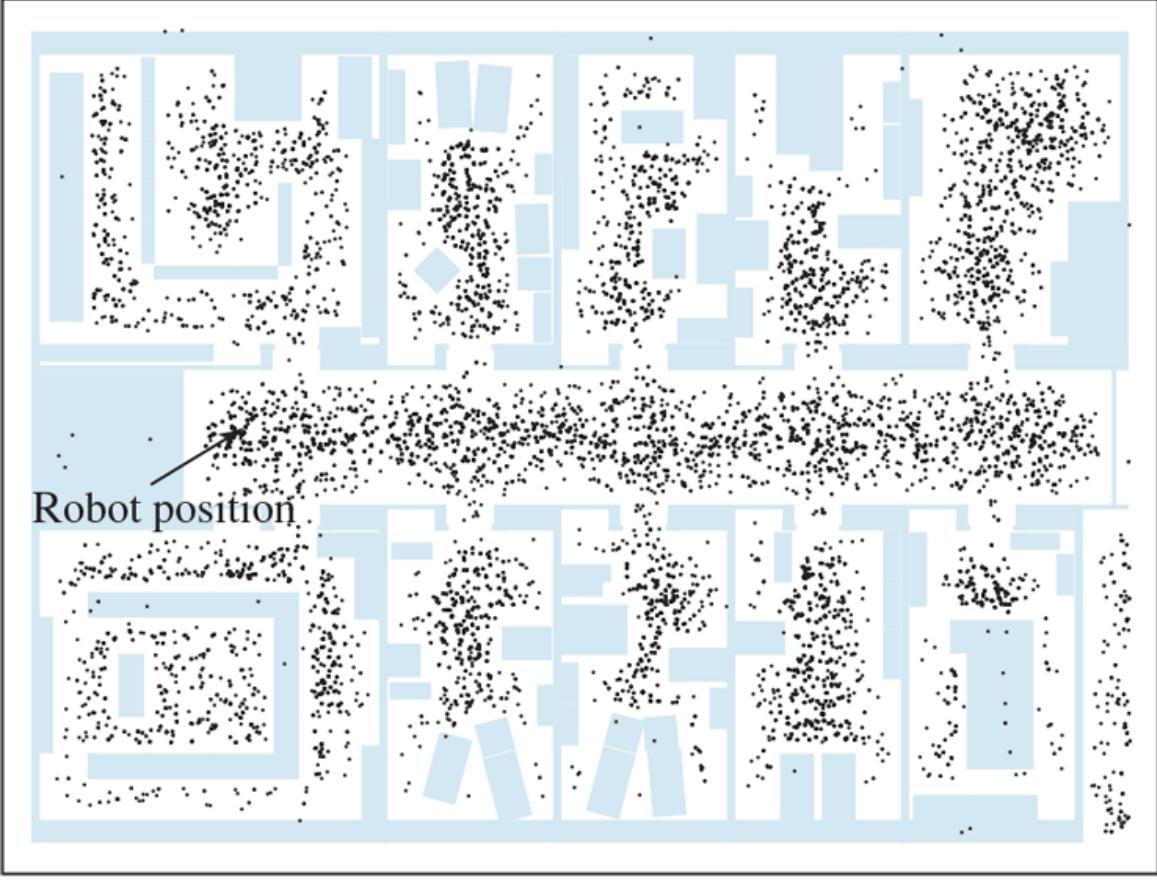
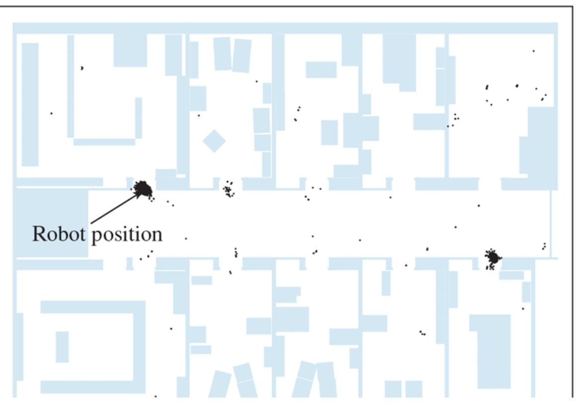
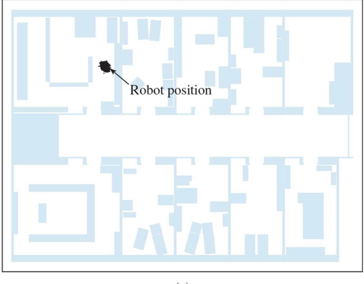
Monte Carlo localization, a particle filtering algorithmformobile robot localization. (a) Initial, global uncertainty. (b) Approximately bimodal uncertainty after navigating in the (symmetric) corridor. (c) Unimodal uncertainty after entering a room and finding it to be distinctive.

The Kalman filter is the other major way to localize. A Kalman filter represents the posterior by a Gaussian. The mean of this Gaussian will be denoted and its covariance The main problem with Gaussian beliefs is that they are closed only under linear motion models and linear measurement models For nonlinear or the result of updating a filter is in general not Gaussian. Thus, localization algorithms using the Kalman filter linearize the motion and sensor models. Linearization is a local approximation of a nonlinear function by a linear function. Figure 26.8 illustrates the concept of linearization for a (one-dimensional) robot motion model. On the left, it depicts a nonlinear motion

model (the control is omitted in this graph since it plays no role in the linearization). On the right, this function is approximated by a linear function This linear function is tangent to at the point the mean of our state estimate at time Such a linearization is called first degree Taylor expansion. A Kalman filter that linearizes and via Taylor expansion is called an extended Kalman filter (or EKF). Figure 26.9 shows a sequence of estimates of a robot running an extended Kalman filter localization algorithm.

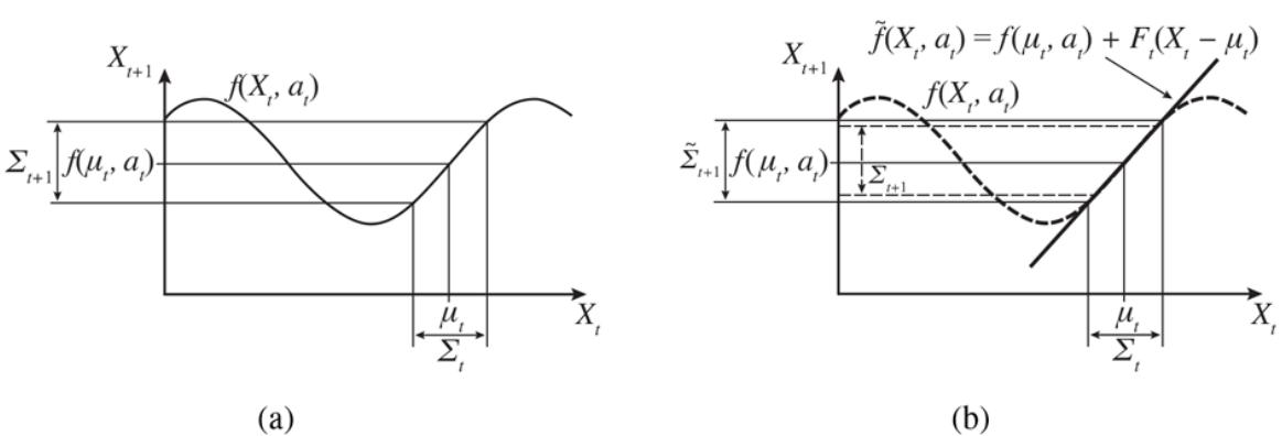
One-dimensional illustration of a linearized motion model: (a) The function and the projection of a mean and a covariance interval (based on ) into time (b) The linearized version is the tangent of at The projection of the mean is correct. However, the projected covariance differs from

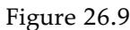
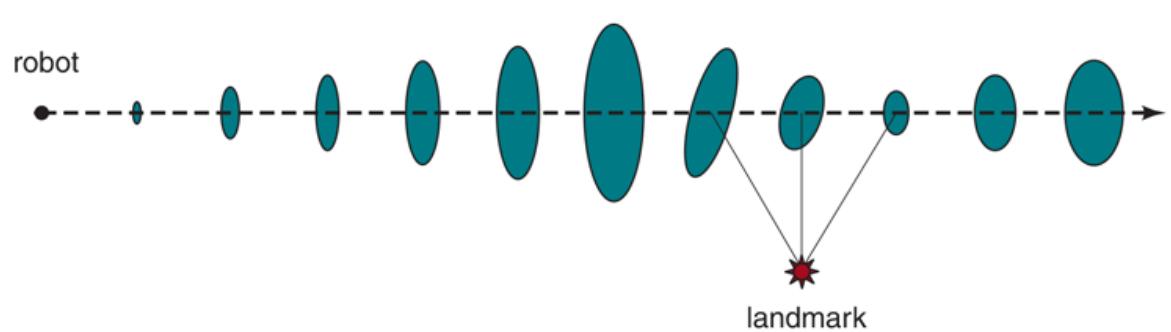
Localization using the extended Kalman filter. The robot moves on a straight line. As it progresses, its uncertainty in its location estimate increases, as illustrated by the error ellipses. When it observes a landmark with known position, the uncertainty is reduced.

Linearization

Taylor expansion

As the robot moves, the uncertainty in its location estimate increases, as shown by the error ellipses. Its error decreases as it senses the range and bearing to a landmark with known location and increases again as the robot loses sight of the landmark. EKF algorithms work well if landmarks are easily identified. Otherwise, the posterior distribution may be multimodal, as in Figure 26.7(b) . The problem of needing to know the identity of landmarks is an instance of the data association problem discussed in Figure 15.3 .

In some situations, no map of the environment is available. Then the robot will have to acquire a map. This is a bit of a chicken-and-egg problem: the navigating robot will have to determine its location relative to a map it doesn’t quite know, at the same time building this map while it doesn’t quite know its actual location. This problem is important for many robot applications, and it has been studied extensively under the name simultaneous localization and mapping, abbreviated as SLAM.

Simultaneous localization and mapping

SLAM problems are solved using many different probabilistic techniques, including the extended Kalman filter discussed above. Using the EKF is straightforward: just augment the state vector to include the locations of the landmarks in the environment. Luckily, the EKF update scales quadratically, so for small maps (e.g., a few hundred landmarks) the computation is quite feasible. Richer maps are often obtained using graph relaxation methods, similar to the Bayesian network inference techniques discussed in Chapter 13 . Expectation–maximization is also used for SLAM.

26.4.2 Other types of perception

Not all of robot perception is about localization or mapping. Robots also perceive temperature, odors, sound, and so on. Many of these quantities can be estimated using variants of dynamic Bayes networks. All that is required for such estimators are conditional probability distributions that characterize the evolution of state variables over time, and sensor models that describe the relation of measurements to state variables.

It is also possible to program a robot as a reactive agent, without explicitly reasoning about probability distributions over states. We cover that approach in Section 26.9.1 .

The trend in robotics is clearly towards representations with well-defined semantics. Probabilistic techniques outperform other approaches in many hard perceptual problems such as localization and mapping. However, statistical techniques are sometimes too cumbersome, and simpler solutions may be just as effective in practice. To help decide which approach to take, experience working with real physical robots is your best teacher.

26.4.3 Supervised and unsupervised learning in robot perception

Machine learning plays an important role in robot perception. This is particularly the case when the best internal representation is not known. One common approach is to map highdimensional sensor streams into lower-dimensional spaces using unsupervised machine learning methods (see Chapter 19 ). Such an approach is called low-dimensional embedding. Machine learning makes it possible to learn sensor and motion models from data, while simultaneously discovering a suitable internal representation.

Low-dimensional embedding

Another machine learning technique enables robots to continuously adapt to big changes in sensor measurements. Picture yourself walking from a sunlit space into a dark room with neon lights. Clearly, things are darker inside. But the change of light source also affects all the colors: neon light has a stronger component of green light than sunlight has. Yet somehow we seem not to notice the change. If we walk together with people into a neon-lit room, we don’t think that their faces suddenly turned green. Our perception quickly adapts to the new lighting conditions, and our brain ignores the differences.

Adaptive perception techniques enable robots to adjust to such changes. One example is shown in Figure 26.10 , taken from the autonomous driving domain. Here an unmanned ground vehicle adapts its classifier of the concept “drivable surface.” How does this work? The robot uses a laser to provide classification for a small area immediately in front of the robot. When this area is found to be flat in the laser range scan, it is used as a positive training example for the concept “drivable surface.” A mixture-of-Gaussians technique similar to the EM algorithm discussed in Chapter 20 is then trained to recognize the specific color and texture coefficients of the small sample patch. The images in Figure 26.10 are the result of applying this classifier to the full image.

Figure 26.10

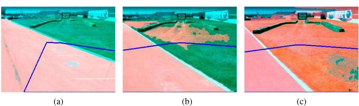
Sequence of “drivable surface” classifications using adaptive vision. (a) Only the road is classified as drivable (pink area). The V-shaped blue line shows where the vehicle is heading. (b) The vehicle is commanded to drive off the road, and the classifier is beginning to classify some of the grass as drivable. (c) The vehicle has updated its model of drivable surfaces to correspond to grass as well as road. Courtesy of Sebastian Thrun.

Methods that make robots collect their own training data (with labels!) are called selfsupervised. In this instance, the robot uses machine learning to leverage a short-range sensor that works well for terrain classification into a sensor that can see much farther. That allows the robot to drive faster, slowing down only when the sensor model says there is a change in the terrain that needs to be examined more carefully by the short-range sensors.

Self-supervised learning

26.5 Planning and Control

The robot’s deliberations ultimately come down to deciding how to move, from the abstract task level all the way down to the currents that are sent to its motors. In this section, we simplify by assuming that perception (and, where needed, prediction) are given, so the world is observable. We further assume deterministic transitions (dynamics) of the world.

We start by separating motion from control. We define a path as a sequence of points in geometric space that a robot (or a robot part, such as an arm) will follow. This is related to the notion of path in Chapter 3 , but here we mean a sequence of points in space rather than a sequence of discrete actions. The task of finding a good path is called motion planning.

Path

Once we have a path, the task of executing a sequence of actions to follow the path is called trajectory tracking control. A trajectory is a path that has a time associated with each point on the path. A path just says “go from A to B to C, etc.” and a trajectory says “start at A, take 1 second to get to B, and another 1.5 seconds to get to C, etc.”

Trajectory tracking control

Trajectory

26.5.1 Configuration space

Imagine a simple robot, in the shape of a right triangle as shown by the lavender triangle in the lower left corner of Figure 26.11 . The robot needs to plan a path that avoids a rectangular obstacle, The physical space that a robot moves about in is called the workspace. This particular robot can move in any direction in the plane, but cannot rotate. The figure shows five other possible positions of the robot with dashed outlines; these are each as close to the obstacle as the robot can get.

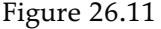
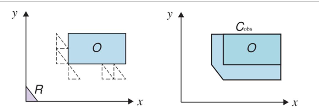
A simple triangular robot that can translate, and needs to avoid a rectangular obstacle. On the left is the workspace, on the right is the configuration space.

Workspace

The body of the robot could be represented as a set of points (or points for a three-dimensional robot), as could the obstacle. With this representation, avoiding the obstacle means that no point on the robot overlaps any point on the obstacle. Motion planning would require calculations on sets of points, which can be complicated and timeconsuming.

We can simplify the calculations by using a representation scheme in which all the points that comprise the robot are represented as a single point in an abstract multidimensional space, which we call the configuration space, or C-space. The idea is that the set of points that comprise the robot can be computed if we know (1) the basic measurements of the robot (for our triangle robot, the length of the three sides will do) and (2) the current pose of the robot—its position and orientation.

Configuration space

C-space

For our simple triangular robot, two dimensions suffice for the C-space: if we know the coordinates of a specific point on the robot—we’ll use the right-angle vertex—then we can calculate where every other point of the triangle is (because we know the size and shape of the triangle and because the triangle cannot rotate). In the lower-left corner of Figure 26.11 , the lavender triangle can be represented by the configuration

If we change the rules so that the robot can rotate, then we will need three dimensions, to be able to calculate where every point is. Here is the robot’s angle of rotation in the plane. If the robot also had the ability to stretch itself, growing uniformly by a scaling factor then the C-space would have four dimensions,

For now we’ll stick with the simple two-dimensional C-space of the non-rotating triangle robot. The next task is to figure out where the points in the obstacle are in C-space. Consider the five dashed-line triangles on the left of Figure 26.11 and notice where the right-angle vertex is on each of these. Then imagine all the ways that the triangle could slide about. Obviously, the right-angle vertex can’t go inside the obstacle, and neither can it get any closer than it is on any of the five dashed-line triangles. So you can see that the area where the right-angle vertex can’t go—the C-space obstacle—is the five-sided polygon on the right of Figure 26.11 labeled

C-space obstacle

In everyday language we speak of there being multiple obstacles for the robot—a table, a chair, some walls. But the math notation is a bit easier if we think of all of these as

combining into one “obstacle” that happens to have disconnected components. In general, the C-space obstacle is the set of all points in such that, if the robot were placed in that configuration, its workspace geometry would intersect the workspace obstacle.

Let the obstacles in the workspace be the set of points and let the set of all points on the robot in configuration be Then the C-space obstacle is defined as

\[C\_{obs} = \{ q: q \in C \text{ and} A(q) \cap O \neq \{ \} \}\]

and the free space is

Free space

The C-space becomes more interesting for robots with moving parts. Consider the two-link arm from Figure 26.12(a) . It is bolted to a table so the base does not move, but the arm has two joints that move independently—we call these degrees of freedom (DOF). Moving the joints alters the coordinates of the elbow, the gripper, and every point on the arm. The arm’s configuration space is two-dimensional: where is the angle of the shoulder joint, and is the angle of the elbow joint.

Figure 26.12

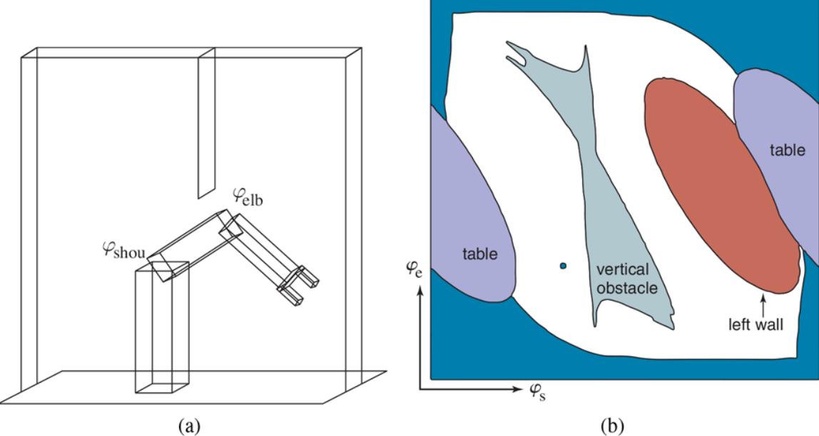
1. Workspace representation of a robot arm with two degrees of freedom. The workspace is a box with a flat obstacle hanging from the ceiling. (b) Configuration space of the same robot. Only white regions in the space are configurations that are free of collisions. The dot in this diagram corresponds to the configuration of the robot shown on the left.

Degrees of freedom (DOF)

Knowing the configuration for our two-link arm means we can determine where each point on the arm is through simple trigonometry. In general, the forward kinematics mapping is a function

\[ \phi\_b: C \to W \]

Forward kinematics

that takes in a configuration and outputs the location of a particular point on the robot when the robot is in that configuration. A particularly useful forward kinematics mapping is that for the robot’s end effector, The set of all points on the robot in a particular configuration is denoted by

\[A(q) = \bigcup\_{b} \{\phi\_b(q)\}.\]

The inverse problem, of mapping a desired location for a point on the robot to the configuration(s) the robot needs to be in for that to happen, is known as inverse kinematics:

\[IK\_b: x \in W \mapsto \{ q \in C \: s.t. \ \phi\_b(q) = x \}\]

Inverse kinematics

Sometimes the inverse kinematics mapping might take not just a position, but also a desired orientation as input. When we want a manipulator to grasp an object, for instance, we can compute a desired position and orientation for its gripper, and use inverse kinematics to determine a goal configuration for the robot. Then a planner needs to find a way to get the robot from its current configuration to the goal configuration without intersecting obstacles.

Workspace obstacles are often depicted as simple geometric forms—especially in robotics textbooks, which tend to focus on polygonal obstacles. But how do the obstacles look in configuration space?

For the two-link arm, simple obstacles in the workspace, like a vertical line, have very complex C-space counterparts, as shown in Figure 26.12(b) . The different shadings of the occupied space correspond to the different objects in the robot’s workspace: the dark region surrounding the entire free space corresponds to configurations in which the robot collides with itself. It is easy to see that extreme values of the shoulder or elbow angles cause such a violation. The two oval-shaped regions on both sides of the robot correspond to the table on which the robot is mounted. The third oval region corresponds to the left wall.

Finally, the most interesting object in configuration space is the vertical obstacle that hangs from the ceiling and impedes the robot’s motions. This object has a funny shape in configuration space: it is highly nonlinear and at places even concave. With a little bit of imagination the reader will recognize the shape of the gripper at the upper left end.

We encourage the reader to pause for a moment and study this diagram. The shape of this obstacle in C-space is not at all obvious! The dot inside Figure 26.12(b) marks the configuration of the robot in Figure 26.12(a) . Figure 26.13 depicts three additional configurations, both in workspace and in configuration space. In configuration conf-1, the gripper is grasping the vertical obstacle.

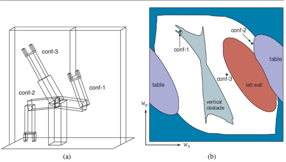
Figure 26.13

Three robot configurations, shown in workspace and configuration space.

We see that even if the robot’s workspace is represented by flat polygons, the shape of the free space can be very complicated. In practice, therefore, one usually probes a configuration space instead of constructing it explicitly. A planner may generate a configuration and then test to see if it is in free space by applying the robot kinematics and then checking for collisions in workspace coordinates.

26.5.2 Motion planning

The motion planning problem is that of finding a plan that takes a robot from one configuration to another without colliding with an obstacle. It is a basic building block for movement and manipulation. In Section 26.5.4 we will discuss how to do this under complicated dynamics, like steering a car that may drift off the path if you take a curve too fast. For now, we will focus on the simple motion planning problem of finding a geometric path that is collision free. Motion planning is a quintessentially continuous-state search problem, but it is often possible to discretize the space and apply the search algorithms from Chapter 3 .

Motion planning

The motion planning problem is sometimes referred to as the piano mover’s problem. It gets its name from a mover’s struggles with getting a large, irregular-shaped piano from one room to another without hitting anything. We are given:

• a workspace world in either for the plane or for three dimensions,
• an obstacle region
• a robot with a configuration space and set of points for
• a starting configuration and
• a goal configuration

Piano mover’problem

The obstacle region induces a C-space obstacle and its corresponding free space defined as in the previous section. We need to find a continuous path through free space. We will use a parameterized curve, to represent the path, where and and for every between 0 and 1 is some point in That is, parameterizes how far we are along the path, from start to goal. Note that acts somewhat like time in that as

increases the distance along the path increases, but is always a point on the interval and is not measured in seconds.

The motion planning problem can be made more complex in various ways: defining the goal as a set of possible configurations rather than a single configuration; defining the goal in the workspace rather than the C-space; defining a cost function (e.g., path length) to be minimized; satisfying constraints (e.g., if the path involves carrying a cup of coffee, making sure that the cup is always oriented upright so the coffee does not spill).

THE SPACES OF MOTION PLANNING: Let’s take a step back and make sure we understand the spaces involved in motion planning. First, there is the workspace or world Points in are points in the everyday three-dimensional world. Next, we have the space of configurations, Points in are -dimensional, with the robot’s number of degrees of freedom, and map to sets of points in Finally, there is the space of paths. The space of paths is a space of functions. Each point in this space maps to an entire curve through C-space. This space is -dimensional! Intuitively, we need dimensions for each configuration along the path, and there are as many configurations on a path as there are points in the number line interval Now let’s consider some ways of solving the motion planning problem.

Visibility graphs

For the simplified case of two-dimensional configuration spaces and polygonal C-space obstacles, visibility graphs are a convenient way to solve the motion planning problem with a guaranteed shortest-path solution. Let be the set of vertices of the polygons making up and let

Visibility graph

We construct a graph on the vertex set with edges connecting a vertex to another vertex if the line connecting the two vertices is collision-free—that is, if When this happens, we say the two vertices “can see each other,” which is where “visibility” graphs got their name.

To solve the motion planning problem, all we need to do is run a discrete graph search (e.g., best-first search) on the graph with starting state and goal In Figure 26.14 we see a visibility graph and an optimal three-step solution. An optimal search on visibility graphs will always give us the optimal path (if one exists), or report failure if no path exists.

Figure 26.14

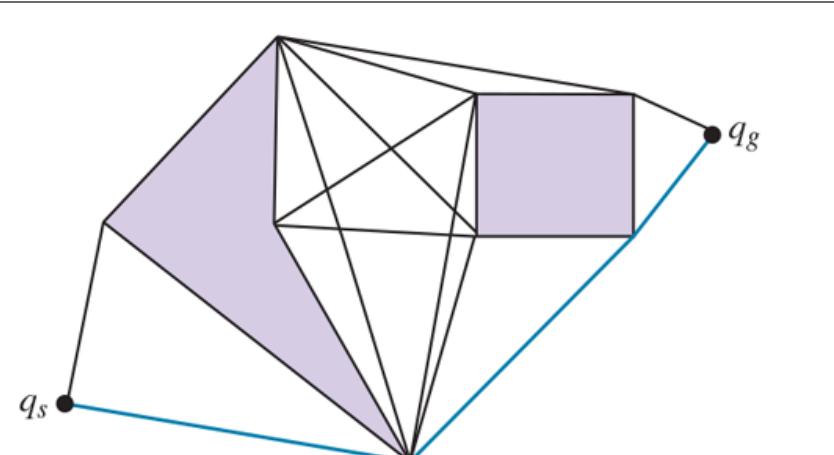
A visibility graph. Lines connect every pair of vertices that can “see” each other—lines that don’t go through an obstacle. The shortest path must lie upon these lines.

Voronoi diagrams

Visibility graphs encourage paths that run immediately adjacent to an obstacle—if you had to walk around a table to get to the door, the shortest path would be to stick as close to the table as possible. However, if motion or sensing is nondeterministic, that would put you at risk of bumping into the table. One way to address this is to pretend that the robot’s body is a bit larger than it actually is, providing a buffer zone. Another way is to accept that path length is not the only metric we want to optimize. Section 26.8.2 shows how to learn a good metric from human examples of behavior.

Figure 26.15

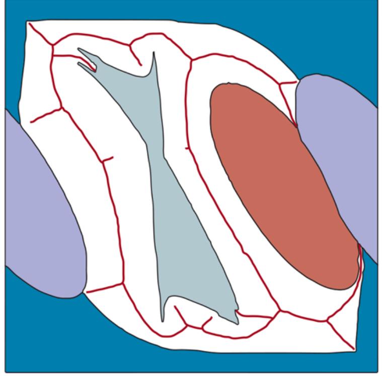
A Voronoi diagram showing the set of points (black lines) equidistant to two or more obstacles in configuration space.

A third way is to use a different technique, one that puts paths as far away from obstacles as possible rather than hugging close to them. A Voronoi diagram is a representation that allows us to do just that. To get an idea for what a Voronoi diagram does, consider a space where the obstacles are, say, a dozen small points scattered about a plane. Now surround each of the obstacle points with a region consisting of all the points in the plane that are closer to that obstacle point than to any other obstacle point. Thus, the regions partition the plane. The Voronoi diagram consists of the set of regions, and the Voronoi graph consists of the edges and vertices of the regions.

Voronoi diagram

Region

Voronoi graph

When obstacles are areas, not points, everything stays pretty much the same. Each region still contains all the points that are closer to one obstacle than to any other, where distance is measured to the closest point on an obstacle. The boundaries between regions still correspond to points that are equidistant between two obstacles, but now the boundary may be a curve rather than a straight line. Computing these boundaries can be prohibitively expensive in high-dimensional spaces.

To solve the motion planning problem, we connect the start point to the closest point on the Voronoi graph via a straight line, and the same for the goal point We then use discrete graph search to find the shortest path on the graph. For problems like navigating through corridors indoors, this gives a nice path that goes down the middle of the corridor. However, in outdoor settings it can come up with inefficient paths, for example suggesting an unnecessary 100 meter detour to stick to the middle of a wide-open 200-meter space.

Cell decomposition

An alternative approach to motion planning is to discretize the -space. Cell decomposition methods decompose the free space into a finite number of contiguous regions, called cells. These cells are designed so that the path-planning problem within a single cell can be solved by simple means (e.g., moving along a straight line). The pathplanning problem then becomes a discrete graph search problem (as with visibility graphs and Voronoi graphs) to find a path through a sequence of cells.

Cell decomposition

The simplest cell decomposition consists of a regularly spaced grid. Figure 26.16(a) shows a square grid decomposition of the space and a solution path that is optimal for this grid size. Grayscale shading indicates the value of each free-space grid cell—the cost of the shortest path from that cell to the goal. (These values can be computed by a deterministic

form of the VALUE-ITERATION algorithm given in Figure 17.6 on page 573.) Figure 26.16(b) shows the corresponding workspace trajectory for the arm. Of course, we could also use the A* algorithm to find a shortest path.

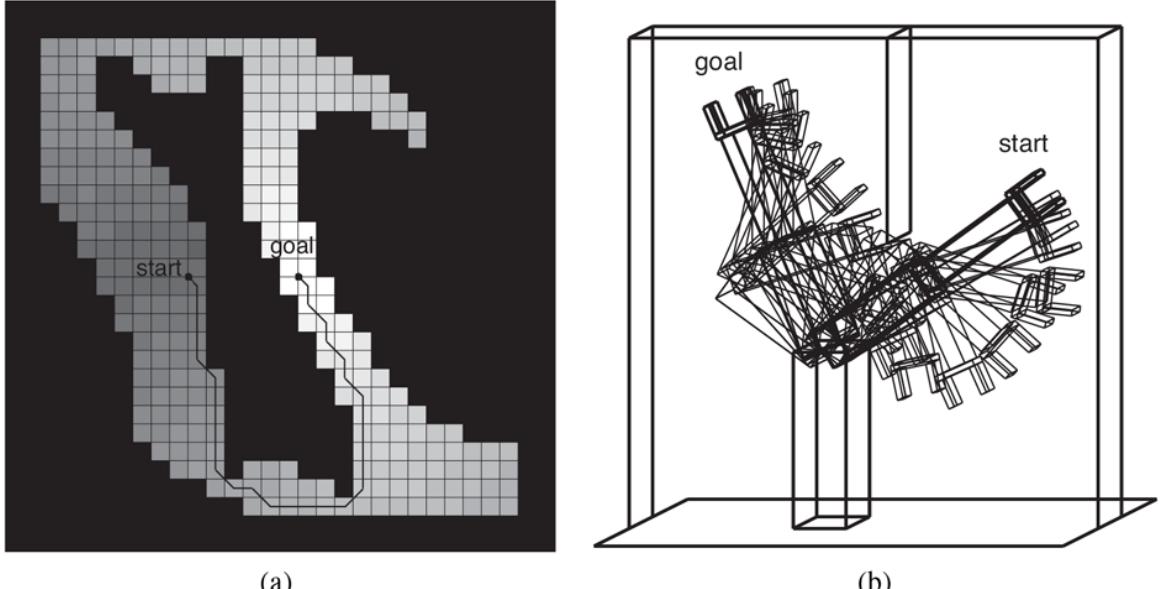
Figure 26.16

This grid decomposition has the advantage that it is simple to implement, but it suffers from three limitations. First, it is workable only for low-dimensional configuration spaces, because the number of grid cells increases exponentially with the number of dimensions. (Sounds familiar? This is the curse of dimensionality.) Second, paths through discretized state space will not always be smooth. We see in Figure 26.16(a) that the diagonal parts of the path are jagged and hence very difficult for the robot to follow accurately. The robot can attempt to smooth out the solution path, but this is far from straightforward.

Third, there is the problem of what to do with cells that are “mixed”—that is, neither entirely within free space nor entirely within occupied space. A solution path that includes such a cell may not be a real solution, because there may be no way to safely cross the cell. This would make the path planner unsound. On the other hand, if we insist that only completely free cells may be used, the planner will be incomplete, because it might be the case that the

only paths to the goal go through mixed cells—it might be that a corridor is actually wide enough for the robot to pass, but the corridor is covered only by mixed cells.

The first approach to this problem is further subdivision of the mixed cells—perhaps using cells of half the original size. This can be continued recursively until a path is found that lies entirely within free cells. This method works well and is complete if there is a way to decide if a given cell is a mixed cell, which is easy only if the configuration space boundaries have relatively simple mathematical descriptions.

It is important to note that cell decomposition does not necessarily require explicitly representing the obstacle space We can decide to include a cell or not by using a collision checker. This is a crucial notion to motion planning. A collision checker is a function that maps to 1 if the configuration collides with an obstacle, and 0 otherwise. It is much easier to check whether a specific configuration is in collision than to explicitly construct the entire obstacle space

Collision checker

Examining the solution path shown in Figure 26.16(a) , we can see an additional difficulty that will have to be resolved. The path contains arbitrarily sharp corners, but a physical robot has momentum and cannot change direction instantaneously. This problem can be solved by storing, for each grid cell, the exact continuous state (position and velocity) that was attained when the cell was reached in the search. Assume further that when propagating information to nearby grid cells, we use this continuous state as a basis, and apply the continuous robot motion model for jumping to nearby cells. So we don’t make an instantaneous turn; we make a rounded turn governed by the laws of motion. We can now guarantee that the resulting trajectory is smooth and can indeed be executed by the robot. One algorithm that implements this is hybrid A*.

Hybrid A*

Randomized motion planning

Randomized motion planning does graph search on a random decomposition of the configuration space, rather than a regular cell decomposition. The key idea is to sample a random set of points and to create edges between them if there is a very simple way to get from one to the other (e.g., via a straight line) without colliding; then we can search on this graph.

A probabilistic roadmap (PRM) algorithm is one way to leverage this idea. We assume access to a collision checker (defined on page 946 ), and to a simple planner that returns a path from to (or failure) but does so quickly. This simple planner is not going to be complete—it might return failure even if a solution actually exists. Its job is to quickly try to connect and and let the main algorithm know if it succeeds. We will use it to define whether an edge exists between two vertices.

Probabilistic roadmap (PRM)

Simple planner

Milestone

The algorithm starts by sampling milestones—points in —in addition to the points and It uses rejection sampling, where configurations are sampled randomly and collisionchecked using until a total of milestones are found. Next, the algorithm uses the simple planner to try to connect pairs of milestones. If the simple planner returns success, then an edge between the pair is added to the graph; otherwise, the graph remains as is. We try to connect each milestone either to its nearest neighbors (we call this -PRM), or to all milestones in a sphere of a radius Finally, the algorithm searches for a path on this graph

from to If no path is found, then more milestones are sampled, added to the graph, and the process is repeated.

Figure 26.17 shows a roadmap with the path found between two configurations. PRMs are not complete, but they are what is called probabilistically complete—they will eventually find a path, if one exists. Intuitively, this is because they keep sampling more milestones. PRMs work well even in high-dimensional configuration spaces.

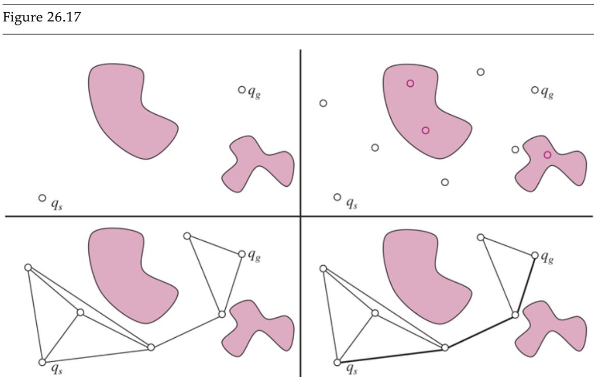
The probabilistic roadmap (PRM) algorithm. Top left: the start and goal configurations. Top right: sample collision-free milestones (here ). Bottom left: connect each milestone to its nearest neighbors (here ). Bottom right: find the shortest path from the start to the goal on the resulting graph.

Probabilistically complete

PRMs are also popular for multi-query planning, in which we have multiple motion planning problems within the same C-space. Often, once the robot reaches a goal, it is called upon to reach another goal in the same workspace. PRMs are really useful, because the robot can dedicate time up front to constructing a roadmap, and amortize the use of that roadmap over multiple queries.

Multi-query planning

Rapidly-exploring random trees

An extension of PRMs called rapidly exploring random trees (RRTs) is popular for singlequery planning. We incrementally build two trees, one with as the root and one with as the root. Random milestones are chosen, and an attempt is made to connect each new milestone to the existing trees. If a milestone connects both trees, that means a solution has been found, as in Figure 26.18 . If not, the algorithm finds the closest point in each tree and adds to the tree a new edge that extends from the point by a distance towards the milestone. This tends to grow the tree towards previously unexplored sections of the space.

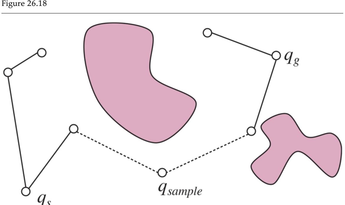
The bidirectional RRT algorithm constructs two trees (one from the start, the other from the goal) by incrementally connecting each sample to the closest node in each tree, if the connection is possible. When a sample connects to both trees, that means we have found a solution path.

Rapidly exploring random trees (RRTs)

Roboticists love RRTs for their ease of use. However, RRT solutions are typically nonoptimal and lack smoothness. Therefore, RRTs are often followed by a post-processing step. The most common one is “short-cutting,” in which we randomly select one of the vertices on the solution path and try to remove it by connecting its neighbors to each other (via the simple planner). We do this repeatedly for as many steps as we have compute time for. Even then, the trajectories might look a little unnatural due to the random positions of the milestone that were selected, as shown in Figure 26.19 .

Figure 26.19

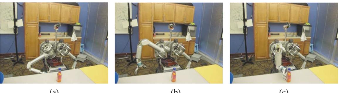
Snapshots of a trajectory produced by an RRT and post-processed with shortcutting. Courtesy of Anca Dragan.

RRT* is a modification to RRT that makes the algorithm asymptotically optimal: the solution converges to the optimal solution as more and more milestones are sampled. The key idea is to pick the nearest neighbor based on a notion of cost to come rather than distance from the milestone only, and to rewire the tree, swapping parents of older vertices if it is cheaper to reach them via the new milestone.

RRT*

Trajectory optimization for kinematic planning

Randomized sampling algorithms tend to first construct a complex but feasible path and then optimize it. Trajectory optimization does the opposite: it starts with a simple but infeasible path, and then works to push it out of collision. The goal is to find a path that optimizes a cost function over paths. That is, we want to minimize the cost function where and 1

1 Roboticists like to minimize a cost function whereas in other parts of AI we try to maximize a utility function or a reward

is called a functional because it is a function over functions. The argument to is which is itself a function: takes as input a point in the interval and maps it to a configuration. A standard cost functional trades off between two important aspects of the robot’s motion: collision avoidance and efficiency,

\[J = J\_{obs} + \lambda J\_{eff}\]

where the efficiency measures the length of the path and may also measure smoothness. A convenient way to define efficiency is with a quadratic: it integrates the squared first derivative of (we will see in a bit why this does in fact incentivize short paths):

\[J\_{eff} = \int\_0^1 \frac{1}{2} \parallel \dot{\tau}(s) \parallel^2 ds.\]

For the obstacle term, assume we can compute the distance from any point to the nearest obstacle edge. This distance is positive outside of obstacles, 0 at the edge, and negative inside. This is called a signed distance field. We can now define a cost field in the workspace, call it that has high cost inside of obstacles, and a small cost right outside. With this cost, we can make points in the workspace really hate being inside obstacles, and dislike being right next to them (avoiding the visibility graph problem of their always hanging out by the edges of obstacles). Of course, our robot is not a point in the workspace, so we have some more work to do—we need to consider all points on the robot’s body:

\[J\_{obs} = \int\_0^1 \int\_b c(\underbrace{\phi\_b(\tau(s))}\_{\in W}) \parallel \frac{d}{ds} \underbrace{\phi\_b(\tau(s))}\_{\in W} \parallel \, db \, ds.\]

Signed distance field

This is called a path integral—it does not just integrate along the way for each body point, but it multiplies by the derivative to make the cost invariant to retiming of the path. Imagine a robot sweeping through the cost field, accumulating cost as is moves. Regardless of how fast or slow the arm moves through the field, it must accumulate the exact same cost.

Path integral

The simplest way to solve the optimization problem above and find a path is gradient descent. If you are wondering how to take gradients of functionals with respect to functions, something called the calculus of variations is here to help. It is especially easy for functionals of the form

\[J[\tau] = \int\_0^1 F(s, \tau(s), \dot{\tau}(s)) ds\]

which are integrals of functions that depend just on the parameter the value of the function at and the derivative of the function at In such a case, the Euler-Lagrange equation says that the gradient is

\[\nabla\_{\tau} J(s) = \frac{\partial F}{\partial \tau(s)}(s) - \frac{d}{dt} \frac{\partial F}{\partial \dot{\tau}(s)}(s).\]

Euler-Lagrange equation

If we look closely at and they both follow this pattern. In particular for we have To get a bit more comfortable with this, let’s compute the gradient for only. We see that does not have a direct dependence on so the first term in the formula is 0. We are left with

\[\nabla\_{\tau} J(s) = 0 - \frac{d}{dt} \dot{\tau}(s)\]

since the partial of with respect to is

Notice how we made things easier for ourselves when defining —it’s a nice quadratic of the derivative (and we even put a in front so that the nicely cancels out). In practice, you will see this trick happen a lot for optimization—the art is not just in choosing how to optimize the cost function, but also in choosing a cost function that will play nicely with how you will optimize it. Simplifying our gradient, we get

\[ \nabla\_{\tau} J(s) = -\ddot{\tau}(s). \]

Now, since is a quadratic, setting this gradient to 0 gives us the solution for if we didn’t have to deal with obstacles. Integrating once, we get that the first derivative needs to be constant; integrating again we get that with and determined by the endpoint constraints for and The optimal path with respect to is thus the straight line from start to goal! It is indeed the most efficient way to go from one to the other if there are no obstacles to worry about.

Of course, the addition of is what makes things difficult—and we will spare you deriving its gradient here. The robot would typically initialize its path to be a straight line, which would plow right through some obstacles. It would then calculate the gradient of the cost about the current path, and the gradient would serve to push the path away from the obstacles (Figure 26.20 ). Keep in mind that gradient descent will only find a locally optimal solution—just like hill climbing. Methods such as simulated annealing (Section 4.1.2 ) can be used for exploration, to make it more likely that the local optimum is a good one.

Figure 26.20

Trajectory optimization for motion planning. Two point-obstacles with circular bands of decreasing cost around them. The optimizer starts with the straight line trajectory, and lets the obstacles bend the line away from collisions, finding the minimum path through the cost field.

26.5.3 Trajectory tracking control

Control theory

We have covered how to plan motions, but not how to actually move—to apply current to motors, to produce torque, to move the robot. This is the realm of control theory, a field of increasing importance in AI. There are two main questions to deal with: how do we turn a mathematical description of a path into a sequence of actions in the real world (open-loop control), and how do we make sure that we are staying on track (closed-loop control)?

Figure 26.21

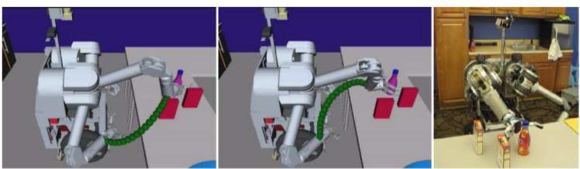
The task of reaching to grasp a bottle solved with a trajectory optimizer. Left: the initial trajectory, plotted for the end effector. Middle: the final trajectory after optimization. Right: the goal configuration. Courtesy of Anca Dragan. See Ratliff et al., (2009).

FROM CONFIGURATIONS TO TORQUES FOR OPEN-LOOP TRACKING: Our path gives us configurations. The robot starts at rest at From there the robot’s motors will turn currents into torques, leading to motion. But what torques should the robot aim for, such that it ends up at

This is where the idea of a dynamics model (or transition model) comes in. We can give the robot a function that computes the effects torques have on the configuration. Remember from physics? Well, there is something like that for torques too, in the form with a torque, a velocity, and an acceleration. If the robot is at configuration and velocity and applied torque that would lead to acceleration The tuple is a dynamic state, because it includes velocity, whereas is the kinematic state and is not sufficient for computing exactly what torque to apply. is a deterministic dynamics model in the MDP over dynamic states with torques as actions. is the inverse dynamics, telling us what torque to apply if we want a particular acceleration, which leads to a change in velocity and thus a change in dynamic state. 2

2 We omit the details of here, but they involve mass, inertia, gravity, and Coriolis and centrifugal forces.

Dynamics model

Dynamic state

Kinematic state

Inverse dynamics

Now, naively, we could think of as “time” on a scale from 0 to 1 and select our torque using inverse dynamics:

(26.2)

\[u(t) = f^{-1}(\tau(t), \dot{\tau}(t), \ddot{\tau}(t))\]

assuming that the robot starts at In reality though, things are not that easy.

The path was created as a sequence of points, without taking velocities and accelerations into account. As such, the path may not satisfy (the robot starts at 0 velocity), or even that is differentiable (let alone twice differentiable). Further, the meaning of the endpoint “1” is unclear: how many seconds does that map to?

Retiming

In practice, before we even think of tracking a reference path, we usually retime it, that is, transform it into a trajectory that maps the interval for some time duration into points in the configuration space (The symbol is the Greek letter Xi.) Retiming is trickier than you might think, but there are approximate ways to do it, for instance by picking a maximum velocity and acceleration, and using a profile that accelerates to that maximum velocity, stays there as long as it can, and then decelerates back to 0. Assuming we can do this, Equation (26.2) above can be rewritten as

(26.3)

\[u(t) = f^{-1}(\xi(t), \dot{\xi}(t), \ddot{\xi}(t)).\]

Even with the change from to an actual trajectory, the equation of applying torques from above (called a control law) has a problem in practice. Thinking back to the reinforcement learning section, you might guess what it is. The equation works great in the situation where

is exact, but pesky reality gets in the way as usual: in real systems, we can’t measure masses and inertias exactly, and might not properly account for physical phenomena like stiction in the motors (the friction that tends to prevent stationary surfaces from being set in motion—to make them stick). So, when the robot arm starts applying those torques but is wrong, the errors accumulate and you deviate further and further from the reference path.

Control law

Stiction

Rather than just letting those errors accumulate, a robot can use a control process that looks at where it thinks it is, compares that to where it wanted to be, and applies a torque to minimize the error.

A controller that provides force in negative proportion to the observed error is known as a proportional controller or P controller for short. The equation for the force is:

\[u(t) = K\_P(\xi(t) - q\_t)\]

P controller

where is the current configuration, and is a constant representing the gain factor of the controller. regulates how strongly the controller corrects for deviations between the actual state and the desired state

Gain factor

Figure 26.22(a) illustrates what can go wrong with proportional control. Whenever a deviation occurs—whether due to noise or to constraints on the forces the robot can apply the robot provides an opposing force whose magnitude is proportional to this deviation. Intuitively, this might appear plausible, since deviations should be compensated by a counterforce to keep the robot on track. However, as Figure 26.22(a) illustrates, a proportional controller can cause the robot to apply too much force, overshooting the desired path and zig-zagging back and forth. This is the result of the natural inertia of the robot: once driven back to its reference position the robot has a velocity that can’t instantaneously be stopped.

Figure 26.22

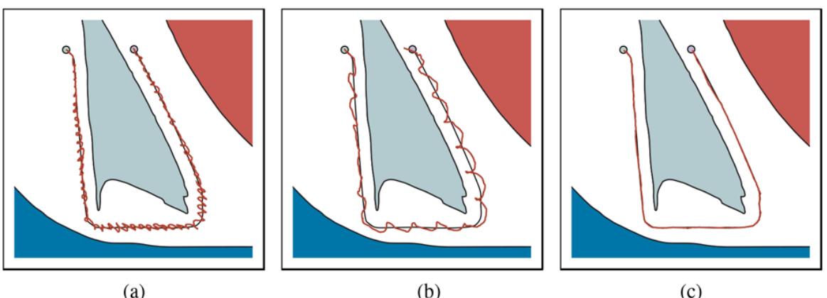
Robot arm control using (a) proportional control with gain factor 1.0, (b) proportional control with gain factor 0.1, and (c) PD (proportional derivative) control with gain factors 0.3 for the proportional component and 0.8 for the differential component. In all cases the robot arm tries to follow the smooth line path, but in (a) and (b) deviates substantially from the path.

In Figure 26.22(a) , the parameter At first glance, one might think that choosing a smaller value for would remedy the problem, giving the robot a gentler approach to the desired path. Unfortunately, this is not the case. Figure 26.22(b) shows a trajectory for still exhibiting oscillatory behavior. The lower value of the gain parameter helps, but does not solve the problem. In fact, in the absence of friction, the P controller is essentially a spring law; so it will oscillate indefinitely around a fixed target location.

There are a number of controllers that are superior to the simple proportional control law. A controller is said to be stable if small perturbations lead to a bounded error between the

robot and the reference signal. It is said to be strictly stable if it is able to return to and then stay on its reference path upon such perturbations. Our P controller appears to be stable but not strictly stable, since it fails to stay anywhere near its reference trajectory.

Stable

Strictly stable

The simplest controller that achieves strict stability in our domain is a PD controller. The letter ‘P’ stands again for proportional, and ‘D’ stands for derivative. PD controllers are described by the following equation:

(26.4)

\[u(t) = K\_P(\xi(t) - q\_t) + K\_D(\dot{\xi}(t) - \dot{q}\_t).\]

PD controller

As this equation suggests, PD controllers extend P controllers by a differential component, which adds to the value of a term that is proportional to the first derivative of the error over time. What is the effect of such a term? In general, a derivative term dampens the system that is being controlled. To see this, consider a situation where the error is changing rapidly over time, as is the case for our P controller above. The derivative of this error will then counteract the proportional term, which will reduce the overall response to the perturbation. However, if the same error persists and does not change, the derivative will vanish and the proportional term dominates the choice of control.

Figure 26.22(c) shows the result of applying this PD controller to our robot arm, using as gain parameters and Clearly, the resulting path is much smoother, and does not exhibit any obvious oscillations.

PD controllers do have failure modes, however. In particular, PD controllers may fail to regulate an error down to zero, even in the absence of external perturbations. Often such a situation is the result of a systematic external force that is not part of the model. For example, an autonomous car driving on a banked surface may find itself systematically pulled to one side. Wear and tear in robot arms causes similar systematic errors. In such situations, an over-proportional feedback is required to drive the error closer to zero. The solution to this problem lies in adding a third term to the control law, based on the integrated error over time:

(26.5)

\[u(t) = \ \ K\_P(\xi(t) - q\_t) + K\_I \int\_0^t (\xi(s) - q\_s)ds + K\_D(\dot{\xi}(t) - \dot{q}\_t).\]

Here is a third gain parameter. The term calculates the integral of the error over time. The effect of this term is that long-lasting deviations between the reference signal and the actual state are corrected. Integral terms, then, ensure that a controller does not exhibit systematic long-term error, although they do pose a danger of oscillatory behavior.

PID controller

A controller with all three terms is called a PID controller (for proportional integral derivative). PID controllers are widely used in industry, for a variety of control problems. Think of the three terms as follows—proportional: try harder the farther away you are from the path; derivative: try even harder if the error is increasing; integral: try harder if you haven’t made progress for a long time.

A middle ground between open-loop control based on inverse dynamics and closed-loop PID control is called computed torque control. We compute the torque our model thinks we will need, but compensate for model inaccuracy with proportional error terms:

(26.6)

\[u(t) = \underbrace{f^{-1}(\xi(t), \dot{\xi}(t), \ddot{\xi}(t))}\_{feedback} + \underbrace{m(\xi(t))\left(K\_P(\xi(t) - q\_t) + K\_D(\dot{\xi}(t) - \dot{q}\_t)\right)}\_{feedback}.\]

The first term is called the feedforward component because it looks forward to where the robot needs to go and computes what torque might be required. The second is the feedback component because it feeds the current error in the dynamic state back into the control law. is the inertia matrix at configuration —unlike normal PD control, the gains change with the configuration of the system.

Feedforward component

Feedback component

Plans versus policies

Let’s take a step back and make sure we understand the analogy between what happened so far in this chapter and what we learned in the search, MDP, and reinforcement learning chapters. With motion in robotics, we are really considering an underlying MDP where the states are dynamic states (configuration and velocity), and the actions are control inputs, usually in the form of torques. If you take another look at our control laws above, they are policies, not plans—they tell the robot what action to take from any state it might reach. However, they are usually far from optimal policies. Because the dynamic state is continuous and high dimensional (as is the action space), optimal policies are computationally difficult to extract.

Instead, what we did here is to break up the problem. We come up with a plan first, in a simplified state and action space: we use only the kinematic state, and assume that states are reachable from one another without paying attention to the underlying dynamics. This is motion planning, and it gives us the reference path. If we knew the dynamics perfectly, we could turn this into a plan for the original state and action space with Equation (26.3) .

But because our dynamics model is typically erroneous, we turn it instead into a policy that tries to follow the plan—getting back to it when it drifts away. When doing this, we introduce suboptimality in two ways: first by planning without considering dynamics, and second by assuming that if we deviate from the plan, the optimal thing to do is to return to the original plan. In what follows, we describe techniques that compute policies directly over the dynamic state, avoiding the separation altogether.

26.5.4 Optimal control

Rather than using a planner to create a kinematic path, and only worrying about the dynamics of the system after the fact, here we discuss how we might be able to do it all at once. We’ll take the trajectory optimization problem for kinematic paths, and turn it into true trajectory optimization with dynamics: we will optimize directly over the actions, taking the dynamics (or transitions) into account.

This brings us much closer to what we’ve seen in the search and MDP chapters. If we know the system’s dynamics, then we can find a sequence of actions to execute, as we did in Chapter 3 . If we’re not sure, then we might want a policy, as in Chapter 17 .

In this section, we are looking more directly at the underlying MDP the robot works in. We’re switching from the familiar discrete MDPs to continuous ones. We will denote our dynamic state of the world by as is common practice—the equivalent of in discrete MDPs. Let and be the starting and goal states.

We want to find a sequence of actions that, when executed by the robot, result in stateaction pairs with low cumulative cost. The actions are torques which we denote with for

starting at 0 and ending at Formally, we want to find the sequence of torques that minimize a cumulative cost

(26.7)

\[\min\_{u} \quad \int\_{0}^{T} J(x(t), u(t))dt\]

subject to the constraints

\[\begin{aligned} \forall t, \dot{x}(t) &= f(x(t), u(t)) \\ x(0) &= x\_s, x(T) = x\_g. \end{aligned}\]

How is this connected to motion planning and trajectory tracking control? Well, imagine we take the notion of efficiency and clearance away from the obstacles and put it into the cost function just as we did before in trajectory optimization over kinematic state. The dynamic state is the configuration and velocity, and torques change it via the dynamics from open-loop trajectory tracking. The difference is that now we’re thinking about the configurations and the torques at the same time. Sometimes, we might want to treat collision avoidance as a hard constraint as well, something we’ve also mentioned before when we looked at trajectory optimization for the kinematic state only.

To solve this optimization problem, we can take gradients of —not with respect to the sequence of configurations anymore, but directly with respect to the controls It is sometimes helpful to include the state sequence as a decision variable too, and use the dynamics constraints to ensure that and are consistent. There are various trajectory optimization techniques using this approach; two of them go by the names multiple shooting and direct collocation. None of these techniques will find the global optimal solution, but in practice they can effectively make humanoid robots walk and make autonomous cars drive.

Magic happens when in the problem above, is quadratic and is linear in and We want to minimize

\[\min \int\_0^\infty x^T Q x + u^T R u dt \qquad \text{subject to} \qquad \forall t, \dot{x}(t) = Ax(t) + Bu(t).\]

We can optimize over an infinite horizon rather than a finite one, and we obtain a policy from any state rather than just a sequence of controls. and need to be positive definite matrices for this to work. This gives us the linear quadratic regulator (LQR). With LQR, the optimal value function (called cost to go) is quadratic, and the optimal policy is linear. The policy looks like where finding the matrix requires solving an algebraic Riccati equation—no local optimization, no value iteration, no policy iteration are needed!

Linear quadratic regulator (LQR)

Riccati equation

Iterative LQR (ILQR)

Because of the ease of finding the optimal policy, LQR finds many uses in practice despite the fact that real problems seldom actually have quadratic costs and linear dynamics. A really useful method is called iterative LQR (ILQR), which works by starting with a solution and then iteratively computing a linear approximation of the dynamics and a quadratic approximation of the cost around it, then solving the resulting LQR system to arrive at a new solution. Variants of LQR are also often used for trajectory tracking.

26.6 Planning Uncertain Movements

In robotics, uncertainty arises from partial observability of the environment and from the stochastic (or unmodeled) effects of the robot’s actions. Errors can also arise from the use of approximation algorithms such as particle filtering, which does not give the robot an exact belief state even if the environment is modeled perfectly.

The majority of today’s robots use deterministic algorithms for decision making, such as the path-planning algorithms of the previous section, or the search algorithms that were introduced in Chapter 3 . These deterministic algorithms are adapted in two ways: first, they deal with the continuous state space by turning it into a discrete space (for example with visibility graphs or cell decomposition). Second, they deal with uncertainty in the current state by choosing the most likely state from the probability distribution produced by the state estimation algorithm. That approach makes the computation faster and makes a better fit for the deterministic search algorithms. In this section we discuss methods for dealing with uncertainty that are analogous to the more complex search algorithms covered in Chapter 4 .

Most likely state

First, instead of deterministic plans, uncertainty calls for policies. We already discussed how trajectory tracking control turns a plan into a policy to compensate for errors in dynamics. Sometimes though, if the most likely hypothesis changes enough, tracking the plan designed for a different hypothesis is too suboptimal. This is where online replanning comes in: we can recompute a new plan based on the new belief. Many robots today use a technique called model predictive control (MPC), where they plan for a shorter time horizon, but replan at every time step. (MPC is therefore closely related to real-time search and gameplaying algorithms.) This effectively results in a policy: at every step, we run a planner and take the first action in the plan; if new information comes along, or we end up not where we

expected, that’s OK, because we are going to replan anyway and that will tell us what to do next.

Online replanning

Model predictive control (MPC)

Second, uncertainty calls for information gathering actions. When we consider only the information we have and make a plan based on it (this is called separating estimation from control), we are effectively solving (approximately) a new MDP at every step, corresponding to our current belief about where we are or how the world works. But in reality, uncertainty is better captured by the POMDP framework: there is something we don’t directly observe, be it the robot’s location or configuration, the location of objects in the world, or the parameters of the dynamics model itself—for example, where exactly is the center of mass of link two on this arm?

What we lose when we don’t solve the POMDP is the ability to reason about future information the robot will get: in MDPs we only plan with what we know, not with what we might eventually know. Remember the value of information? Well, robots that plan using their current belief as if they will never find out anything more fail to account for the value of information. They will never take actions that seem suboptimal right now according to what they know, but that will actually result in a lot of information and enable the robot to do well.

What does such an action look like for a navigation robot? The robot could get close to a landmark to get a better estimate of where it is, even if that landmark is out of the way according to what it currently knows. This action is optimal only if the robot considers the new observations it will get, as opposed to looking only at the information it already has.

Guarded movement

To get around this, robotics techniques sometimes define information gathering actions explicitly—such as moving a hand until it touches a surface (called guarded movements) and make sure the robot does that before coming up with a plan for reaching its actual goal. Each guarded motion consists of (1) a motion command and (2) a termination condition, which is a predicate on the robot’s sensor values saying when to stop.

Sometimes, the goal itself could be reached via a sequence of guarded moves guaranteed to succeed regardless of uncertainty. As an example, Figure 26.23 shows a two-dimensional configuration space with a narrow vertical hole. It could be the configuration space for insertion of a rectangular peg into a hole or a car key into the ignition. The motion commands are constant velocities. The termination conditions are contact with a surface. To model uncertainty in control, we assume that instead of moving in the commanded direction, the robot’s actual motion lies in the cone about it.

A two-dimensional environment, velocity uncertainty cone, and envelope of possible robot motions. The intended velocity is but with uncertainty the actual velocity could be anywhere in resulting in a final configuration somewhere in the motion envelope, which means we wouldn’t know if we hit the hole or not.

The figure shows what would happen if the robot attempted to move straight down from the initial configuration. Because of the uncertainty in velocity, the robot could move anywhere in the conical envelope, possibly going into the hole, but more likely landing to one side of

it. Because the robot would not then know which side of the hole it was on, it would not know which way to move.

A more sensible strategy is shown in Figures 26.24 and 26.25 . In Figure 26.24 , the robot deliberately moves to one side of the hole. The motion command is shown in the figure, and the termination test is contact with any surface. In Figure 26.25 , a motion command is given that causes the robot to slide along the surface and into the hole. Because all possible velocities in the motion envelope are to the right, the robot will slide to the right whenever it is in contact with a horizontal surface.

The first motion command and the resulting envelope of possible robot motions. No matter what actual motion ensues, we know the final configuration will be to the left of the hole.

Figure 26.25

The second motion command and the envelope of possible motions. Even with error, we will eventually get into the hole.

It will slide down the right-hand vertical edge of the hole when it touches it, because all possible velocities are down relative to a vertical surface. It will keep moving until it reaches the bottom of the hole, because that is its termination condition. In spite of the control uncertainty, all possible trajectories of the robot terminate in contact with the bottom of the hole—that is, unless surface irregularities cause the robot to stick in one place.

Coastal navigation

Other techniques beyond guarded movements change the cost function to incentivize actions we know will lead to information—like the coastal navigation heuristic which requires the robot to stay near known landmarks. More generally, techniques can incorporate the expected information gain (reduction of entropy of the belief) as a term in the cost function, leading to the robot explicitly reasoning about how much information each action might bring when deciding what to do. While more difficult computationally, such approaches have the advantage that the robot invents its own information gathering actions rather than relying on human-provided heuristics and scripted strategies that often lack flexibility.

26.7 Reinforcement Learning in Robotics

Thus far we have considered tasks in which the robot has access to the dynamics model of the world. In many tasks, it is very difficult to write down such a model, which puts us in the domain of reinforcement learning (RL).

One challenge of RL in robotics is the continuous nature of the state and action spaces, which we handle either through discretization, or, more commonly, through function approximation. Policies or value functions are represented as combinations of known useful features, or as deep neural networks. Neural nets can map from raw inputs directly to outputs, and thus largely avoid the need for feature engineering, but they do require more data.

A bigger challenge is that robots operate in the real world. We have seen how reinforcement learning can be used to learn to play chess or Go by playing simulated games. But when a real robot moves in the real world, we have to make sure that its actions are safe (things break!), and we have to accept that progress will be slower than in a simulation because the world refuses to move faster than one second per second. Much of what is interesting about using reinforcement learning in robotics boils down to how we might reduce the real world sample complexity—the number of interactions with the physical world that the robot needs before it has learned how to do the task.

26.7.1 Exploiting models

A natural way to avoid the need for many real-world samples is to use as much knowledge of the world’s dynamics as possible. For instance, we might not know exactly what the coefficient of friction or the mass of an object is, but we might have equations that describe the dynamics as a function of these parameters.

In such a case, model-based reinforcement learning (Chapter 22 ) is appealing, where the robot can alternate between fitting the dynamics parameters and computing a better policy. Even if the equations are incorrect because they fail to model every detail of physics, researchers have experimented with learning an error term, in addition to the parameters, that can compensate for the inaccuracy of the physical model. Or, we can abandon the

equations and instead fit locally linear models of the world that each approximate the dynamics in a region of the state space, an approach that has been successful in getting robots to master complex dynamic tasks like juggling.

Sim-to-real

A model of the world can also be useful in reducing the sample complexity of model-free reinforcement learning methods by doing sim-to-real transfer: transferring policies that work in simulation to the real world. The idea is to use the model as a simulator for a policy search (Section 22.5 ). To learn a policy that transfers well, we can add noise to the model during training, thereby making the policy more robust. Or, we can train policies that will work with a variety of models by sampling different parameters in the simulations sometimes referred to as domain randomization. An example is in Figure 26.26 , where a dexterous manipulation task is trained in simulation by varying visual attributes, as well as physical attributes like friction or damping.

Figure 26.26

Training a robust policy. (a) Multiple simulations are run of a robot hand manipulating objects, with different randomized parameters for physics and lighting. Courtesy of Wojciech Zaremba. (b) The realworld environment, with a single robot hand in the center of a cage, surrounded by cameras and range

finders. (c) Simulation and real-world training yields multiple different policies for grasping objects; here a pinch grasp and a quadpod grasp. Courtesy of OpenAI. See Andrychowicz et al., (2018a).

Domain randomization

Finally, hybrid approaches that borrow ideas from both model-based and model-free algorithms are meant to give us the best of both. The hybrid approach originated with the Dyna architecture, where the idea was to iterate between acting and improving the policy, but the policy improvement would come in two complementary ways: 1) the standard model-free way of using the experience to directly update the policy, and 2) the modelbased way of using the experience to fit a model, then plan with it to generate a policy.

More recent techniques have experimented with fitting local models, planning with them to generate actions, and using these actions as supervision to fit a policy, then iterating to get better and better models around the areas that the policy needs. This has been successfully applied in end-to-end learning, where the policy takes pixels as input and directly outputs torques as actions—it enabled the first demonstration of deep RL on physical robots.

Models can also be exploited for the purpose of ensuring safe exploration. Learning slowly but safely may be better than learning quickly but crashing and burning half way through. So arguably, more important than reducing real-world samples is reducing real-world samples in dangerous states—we don’t want robots falling off cliffs, and we don’t want them breaking our favorite mugs or, even worse, colliding with objects and people. An approximate model, with uncertainty associated to it (for example by considering a range of values for its parameters), can guide exploration and impose constraints on the actions that the robot is allowed to take in order to avoid these dangerous states. This is an active area of research in robotics and control.

26.7.2 Exploiting other information

Models are useful, but there is more we can do to further reduce sample complexity.

When setting up a reinforcement learning problem, we have to select the state and action spaces, the representation of the policy or value function, and the reward function we’re using. These decisions have a large impact on how easy or how hard we are making the problem.

One approach is to use higher-level motion primitives instead of low-level actions like torque commands. A motion primitive is a parameterized skill that the robot has. For example, a robotic soccer player might have the skill of “pass the ball to the player at” All the policy needs to do is to figure out how to combine them and set their parameters, instead of reinventing them. This approach often learns much faster than low-level approaches, but does restrict the space of possible behaviors that the robot can learn.

Motion primitive

Another way to reduce the number of real-world samples required for learning is to reuse information from previous learning episodes on other tasks, rather than starting from scratch. This falls under the umbrella of metalearning or transfer learning.

Finally, people are a great source of information. In the next section, we talk about how to interact with people, and part of it is how to use their actions to guide the robot’s learning.

26.8 Humans and Robots

Thus far, we’ve focused on a robot planning and learning how to act in isolation. This is useful for some robots, like the rovers we send out to explore distant planets on our behalf. But, for the most part, we do not build robots to work in isolation. We build them to help us, and to work in human environments, around and with us.

This raises two complementary challenges. First is optimizing reward when there are people acting in the same environment as the robot. We call this the coordination problem (see Section 18.1 ). When the robot’s reward depends on not just its own actions, but also the actions that people take, the robot has to choose its actions in a way that meshes well with theirs. When the human and the robot are on the same team, this turns into collaboration.

Second is the challenge of optimizing for what people actually want. If a robot is to help people, its reward function needs to incentivize the actions that people want the robot to execute. Figuring out the right reward function (or policy) for the robot is itself an interaction problem. We will explore these two challenges in turn.

26.8.1 Coordination

Let’s assume for now, as we have been, that the robot has access to a clearly defined reward function. But, instead of needing to optimize it in isolation, now the robot needs to optimize it around a human who is also acting. For example, as an autonomous car merges on the highway, it needs to negotiate the maneuver with the human driver coming in the target lane—should it accelerate and merge in front, or slow down and merge behind? Later, as it pulls to a stop sign, preparing to take a right, it has to watch out for the cyclist in the bicycle lane, and for the pedestrian about to step onto the crosswalk.

Or, consider a mobile robot in a hallway. Someone heading straight toward the robot steps slightly to the right, indicating which side of the robot they want to pass on. The robot has to respond, clarifying its intentions.

Humans as approximately rational agents

One way to formulate coordination with a human is to model it as a game between the robot and the human (Section 18.2 ). With this approach, we explicitly make the assumption that people are agents incentivized by objectives. This does not automatically mean that they are perfectly rational agents (i.e., find optimal solutions in the game), but it does mean that the robot can structure the way it reasons about the human via the notion of possible objectives that the human might have. In this game:

• the state of the environment captures the configurations of both the robot and human agents; call it
• each agent can take actions, and respectively;
• each agent has an objective that can be represented as a cost, and each agent wants to get to its goal safely and efficiently;
• and, as in any game, each objective depends on the state and on the actions of both agents: and Think of the car-pedestrian interaction—the car should stop if the pedestrian crosses, and should go forward if the pedestrian waits.

Incomplete information game

Three important aspects complicate this game. First is that the human and the robot don’t necessarily know each other’s objectives. This makes it an incomplete information game.

Second is that the state and action spaces are continuous, as they’ve been throughout this chapter. We learned in Chapter 5 how to do tree search to tackle discrete games, but how do we tackle continuous spaces?

Third, even though at the high level the game model makes sense—humans do move, and they do have objectives—a human’s behavior might not always be well-characterized as a solution to the game. The game comes with a computational challenge not only for the robot, but for us humans too. It requires thinking about what the robot will do in response to what the person does, which depends on what the robot thinks the person will do, and pretty soon we get to “what do you think I think you think I think”— it’s turtles all the way

down! Humans can’t deal with all of that, and exhibit certain suboptimalities. This means that the robot should account for these suboptimalities.

So, then, what is an autonomous car to do when the coordination problem is this hard? We will do something similar to what we’ve done before in this chapter. For motion planning and control, we took an MDP and broke it up into planning a trajectory and then tracking it with a controller. Here too, we will take the game, and break it up into making predictions about human actions, and deciding what the robot should do given these predictions.

Predicting human action

Predicting human actions is hard because they depend on the robot’s actions and vice versa. One trick that robots use is to pretend the person is ignoring the robot. The robot assumes people are noisily optimal with respect to their objective, which is unknown to the robot and is modeled as no longer dependent on the robot’s actions: In particular, the higher the value of an action for the objective (the lower the cost to go), the more likely the human is to take it. The robot can create a model for for instance using the softmax function from page 811:

(26.8)

\[P(u\_H \mid x, J\_H) \propto e^{-Q(x, u\_H; J\_H)}\]

with the Q-value function corresponding to (the negative sign is there because in robotics we like to minimize cost, not maximize reward). Note that the robot does not assume perfectly optimal actions, nor does it assume that the actions are chosen based on reasoning about the robot at all.

Armed with this model, the robot uses the human’s ongoing actions as evidence about If we have an observation model for how human actions depend on the human’s objective, each human action can be incorporated to update the robot’s belief over what objective the person has:

(26.9)

\[b'(J\_H) \propto b(J\_H)P(u\_H \mid x, J\_H).\]

An example is in Figure 26.27 : the robot is tracking a human’s location and as the human moves, the robot updates its belief over human goals. As the human heads toward the windows, the robot increases the probability that the goal is to look out the window, and decreases the probability that the goal is going to the kitchen, which is in the other direction.

Figure 26.27

Making predictions by assuming that people are noisily rational given their goal: the robot uses the past actions to update a belief over what goal the person is heading to, and then uses the belief to make predictions about future actions. (a) The map of a room. (b) Predictions after seeing a small part of the person’s trajectory (white path); (c) Predictions after seeing more human actions: the robot now knows that the person is not heading to the hallway on the left, because the path taken so far would be a poor path if that were the person’s goal. Images courtesy of Brian D. Ziebart. See Ziebart et al., (2009).

This is how the human’s past actions end up informing the robot about what the human will do in the future. Having a belief about the human’s goal helps the robot anticipate what next actions the human will take. The heatmap in the figure shows the robot’s future predictions: red is most probable; blue least probable.

The same can happen in driving. We might not know how much another driver values efficiency, but if we see them accelerate as someone is trying to merge in front of them, we now know a bit more about them. And once we know that, we can better anticipate what they will do in the future—the same driver is likely to come closer behind us, or weave through traffic to get ahead.

Once the robot can make predictions about human future actions, it has reduced its problem to solving an MDP. The human actions complicate the transition function, but as long as the robot can anticipate what action the person will take from any future state, the robot can calculate it can compute from by marginalizing over and combine it with the transition (dynamics) function for how the

world updates based on both the robot’s and the human’s actions. In Section 26.5 we focused on how to solve this in continuous state and action spaces for deterministic dynamics, and in Section 26.6 we discussed doing it with stochastic dynamics and uncertainty.

Splitting prediction from action makes it easier for the robot to handle interaction, but sacrifices performance much as splitting estimation from motion did, or splitting planning from control.

A robot with this split no longer understands that its actions can influence what people end up doing. In contrast, the robot in Figure 26.27 anticipates where people will go and then optimizes for reaching its own goal and avoiding collisions with them. In Figure 26.28 , we have an autonomous car merging on the highway. If it just planned in reaction to other cars, it might have to wait a long time while other cars occupy its target lane. In contrast, a car that reasons about prediction and action jointly knows that different actions it could take will result in different reactions from the human. If it starts to assert itself, the other cars are likely to slow down a bit and make room. Roboticists are working towards coordinated interactions like this so robots can work better with humans.

Figure 26.28

1. Left: An autonomous car (middle lane) predicts that the human driver (left lane) wants to keep going forward, and plans a trajectory that slows down and merges behind. Right: The car accounts for the influence its actions can have on human actions, and realizes it can merge in front and rely on the human driver to slow down. (b) That same algorithm produces an unusual strategy at an intersection: the car realizes that it can make it more likely for the person (bottom) to proceed faster through the intersection by starting to inch backwards. Images courtesy of Anca Dragan. See Sadigh et al., (2016).

Human predictions about the robot

Incomplete information is often two-sided: the robot does not know the human’s objective and the human, in turn, does not know the robot’s objective—people need to be making predictions about robots. As robot designers, we are not in charge of how the human makes predictions; we can only control what the robot does. However, the robot can act in a way to make it easier for the human to make correct predictions. The robot can assume that the human is using something roughly analogous to Equation (26.8) to estimate the robot’s objective and thus the robot will act so that its true objective can be easily inferred.

A special case of the game is when the human and the robot are on the same team, working toward the same goal or objective: Imagine getting a personal home robot that is helping you make dinner or clean up—these are examples of collaboration.

We can now define a joint agent whose actions are tuples of human–robot actions, and who optimizes for and we’re solving a regular planning problem. We compute the optimal plan or policy for the joint agent, and voila, we now know what the robot and human should do.

Joint agent

This would work really well if people were perfectly optimal. The robot would do its part of the joint plan, the human theirs. Unfortunately, in practice, people don’t seem to follow the perfectly laid out joint-agent plan; they have a mind of their own! We’ve already learned one way to handle this though, back in Section 26.6 . We called it model predictive control (MPC): the idea was to come up with a plan, execute the first action, and then replan. That way, the robot always adapts its plan to what the human is actually doing.

Let’s work through an example. Suppose you and the robot are in your kitchen, and have decided to make waffles. You are slightly closer to the fridge, so the optimal joint plan would have you grab the eggs and milk from the fridge, while the robot fetches the flour from the cabinet. The robot knows this because it can measure quite precisely where everyone is. But suppose you start heading for the flour cabinet. You are going against the optimal joint plan. Rather than sticking to it and stubbornly also going for the flour, the MPC robot recalculates the optimal plan, and now that you are close enough to the flour it is best for the robot to grab the waffle iron instead.

If we know that people might deviate from optimality, we can account for it ahead of time. In our example, the robot can try to anticipate that you are going for the flour the moment you take your first step (say, using the prediction technique above). Even if it is still technically optimal for you to turn around and head for the fridge, the robot should not assume that’s what is going to happen. Instead, the robot can compute a plan in which you keep doing what you seem to want.

Humans as black box agents

We don’t have to treat people as objective-driven, intentional agents to get robots to coordinate with us. An alternative model is that the human is merely some agent whose policy “messes” with the environment dynamics. The robot does not know but can model the problem as needing to act in an MDP with unknown dynamics. We have seen this before: for general agents in Chapter 22 , and for robots in particular in Section 26.7 .

The robot can fit a policy model to human data, and use it to compute an optimal policy for itself. Due to scarcity of data, this has been mostly used so far at the task level. For instance, robots have learned through interaction what actions people tend to take (in response to its own actions) for the task of placing and drilling screws in an industrial assembly task.

Then there is also the model-free reinforcement learning alternative: the robot can start with some initial policy or value function, and keep improving it over time via trial and error.

26.8.2 Learning to do what humans want

Another way interaction with humans comes into robotics is in itself—the robot’s cost or reward function. The framework of rational agents and the associated algorithms reduce the problem of generating good behavior to specifying a good reward function. But for robots, as for many other AI agents, getting the cost right is still difficult.

Take autonomous cars: we want them to reach the destination, to be safe, to drive comfortably for their passengers, to obey traffic laws, etc. A designer of such a system needs to trade off these different components of the cost function. The designer’s task is hard because robots are built to help end users, and not every end user is the same. We all have different preferences for how aggressively we want our car to drive, etc.

Below, we explore two alternatives for trying to get robot behavior to match what we actually want the robot to do. The first is to learn a cost function from human input. The second is to bypass the cost function and imitate human demonstrations of the task.

Preference learning: Learning cost functions

Imagine that an end user is showing a robot how to do a task. For instance, they are driving the car in the way they would like it to be driven by the robot. Can you think of a way for the robot to use these actions—we call them “demonstrations”—to figure out what cost function it should optimize?

We have actually already seen the answer to this back in Section 26.8.1 . There, the setup was a little different: we had another person taking actions in the same space as the robot, and the robot needed to predict what the person would do. But one technique we went over for making these predictions was to assume that people act to noisily optimize some cost function and we can use their ongoing actions as evidence about what cost function that is. We can do the same here, except not for the purpose of predicting human behavior in the future, but rather acquiring the cost function the robot itself should optimize. If the person drives defensively, the cost function that will explain their actions will put a lot of weight on safety and less so on efficiency. The robot can adopt this cost function as its own and optimize it when driving the car itself.

Roboticists have experimented with different algorithms for making this cost inference computationally tractable. In Figure 26.29 , we see an example of teaching a robot to prefer staying on the road to going over the grassy terrain. Traditionally in such methods, the cost function has been represented as a combination of hand-crafted features, but recent work has also studied how to represent it using a deep neural network, without feature engineering.

Left: A mobile robot is shown a demonstration that stays on the dirt road. Middle: The robot infers the desired cost function, and uses it in a new scene, knowing to put lower cost on the road there. Right: The robot plans a path for the new scene that also stays on the road, reproducing the preferences behind the demonstration. Images courtesy of Nathan Ratliff and James A. Bagnell. See Ratliff et al., (2006).

There are other ways for a person to provide input. A person could use language rather than demonstration to instruct the robot. A person could act as a critic, watching the robot perform a task one way (or two ways) and then saying how well the task was done (or which way was better), or giving advice on how to improve.

Learning policies directly via imitation

An alternative is to bypass cost functions and learn the desired robot policy directly. In our car example, the human’s demonstrations make for a convenient data set of states labeled by the action the robot should take at each state: The robot can run supervised learning to fit a policy and execute that policy. This is called imitation learning or behavioral cloning.

Behavioral cloning

Generalization

A challenge with this approach is in generalization to new states. The robot does not know why the actions in its database have been marked as optimal. It has no causal rule; all it can do is run a supervised learning algorithm to try to learn a policy that will generalize to unknown states. However, there is no guarantee that the generalization will be correct.

Figure 26.30

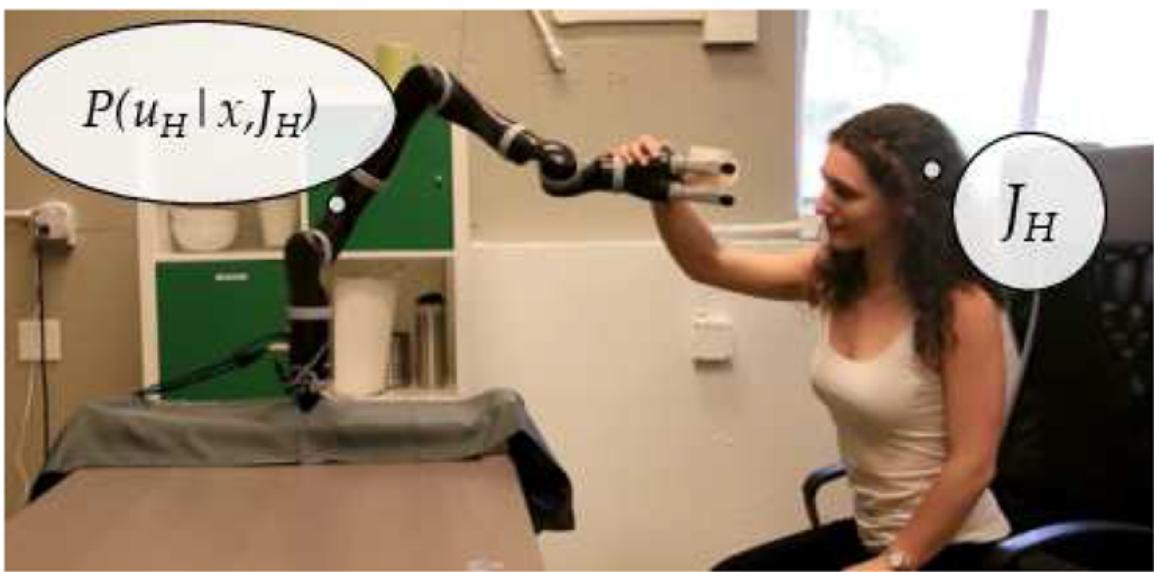
A human teacher pushes the robot down to teach it to stay closer to the table. The robot appropriately updates its understanding of the desired cost function and starts optimizing it. Courtesy of Anca Dragan. See Bajcsy et al., (2017).

The ALVINN autonomous car project used this approach, and found that even when starting from a state in will make small errors, which will take the car off the demonstrated trajectory. There, will make a larger error, which will take the car even further off the desired course.

We can address this at training time if we interleave collecting labels and learning: start with a demonstration, learn a policy, then roll out that policy and ask the human for what action to take at every state along the way, then repeat. The robot then learns how to correct its mistakes as it deviates from the human’s desired actions.

Alternatively, we can address it by leveraging reinforcement learning. The robot can fit a dynamics model based on the demonstrations, and then use optimal control (Section 26.5.4 ) to generate a policy that optimizes for staying close to the demonstration. A version of this has been used to perform very challenging maneuvers at an expert level in a small radio-controlled helicopter (see Figure 22.9(b) ).

The DAGGER (Data Aggregation) system starts with a human expert demonstration. From that it learns a policy, and uses the policy to generate a data set Then from it

generates a new policy that best imitates the original human data. This repeats, and on the th iteration it uses to generate more data, to be added to which is then used to create In other words, at each iteration the system gathers new data under the current policy and trains the next policy using all the data gathered so far.

Related recent techniques use adversarial training: they alternate between training a classifier to distinguish between the robot’s learned policy and the human’s demonstrations, and training a new robot policy via reinforcement learning to fool the classifier. These advances enable the robot to handle states that are near demonstrations, but generalization to far-off states or to new dynamics is a work in progress.

Teaching interfaces and the correspondence problem. So far, we have imagined the case of an autonomous car or an autonomous helicopter, for which human demonstrations use the same actions that the robot can take itself: accelerating, braking, and steering. But what happens if we do this for tasks like cleaning up the kitchen table? We have two choices here: either the person demonstrates using their own body while the robot watches, or the person physically guides the robot’s effectors.

The first approach is appealing because it comes naturally to end users. Unfortunately, it suffers from the correspondence problem: how to map human actions onto robot actions. People have different kinematics and dynamics than robots. Not only does that make it difficult to translate or retarget human motion onto robot motion (e.g., retargeting a fivefinger human grasp to a two-finger robot grasp), but often the high-level strategy a person might use is not appropriate for the robot.

Correspondence problem

The second approach, where the human teacher moves the robot’s effectors into the right positions, is called kinesthetic teaching. It is not easy for humans to teach this way, especially to teach robots with multiple joints. The teacher needs to coordinate all the degrees of freedom as it is guiding the arm through the task. Researchers have thus investigated alternatives, like demonstrating keyframes as opposed to continuous

trajectories, as well as the use of visual programming to enable end users to program primitives for a task rather than demonstrate from scratch (Figure 26.31 ). Sometimes both approaches are combined.

Figure 26.31

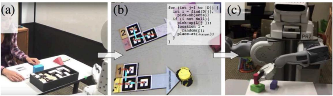
A programming interface that involves placing specially designed blocks in the robot’s workspace to select objects and specify high-level actions. Images courtesy of Maya Cakmak. See Sefidgar et al., (2017).

Kinesthetic teaching

Keyframe

Visual programming

26.9 Alternative Robotic Frameworks

Thus far, we have taken a view of robotics based on the notion of defining or learning a reward function, and having the robot optimize that reward function (be it via planning or learning), sometimes in coordination or collaboration with humans. This is a deliberative view of robotics, to be contrasted with a reactive view.

Deliberative

Reactive

26.9.1 Reactive controllers

In some cases, it is easier to set up a good policy for a robot than to model the world and plan. Then, instead of a rational agent, we have a reflex agent.

For example, picture a legged robot that attempts to lift a leg over an obstacle. We could give this robot a rule that says lift the leg a small height and move it forward, and if the leg encounters an obstacle, move it back and start again at a higher height. You could say that is modeling an aspect of the world, but we can also think of as an auxiliary variable of the robot controller, devoid of direct physical meaning.

One such example is the six-legged (hexapod) robot, shown in Figure 26.32(a) , designed for walking through rough terrain. The robot’s sensors are inadequate to obtain accurate models of the terrain for path planning. Moreover, even if we added high-precision cameras and rangefinders, the 12 degrees of freedom (two for each leg) would render the resulting path planning problem computationally difficult.

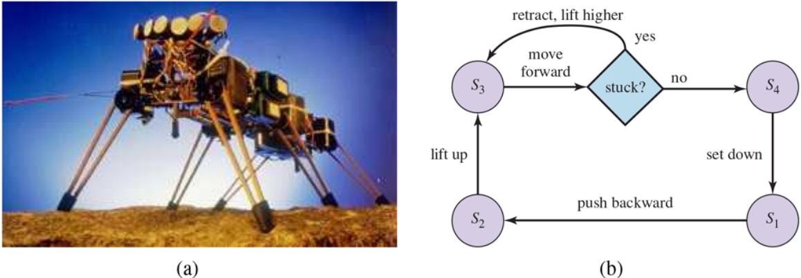
1. Genghis, a hexapod robot. (Image courtesy of Rodney A. Brooks.) (b) An augmented finite state machine (AFSM) that controls one leg. The AFSM reacts to sensor feedback: if a leg is stuck during the forward swinging phase, it will be lifted increasingly higher.

It is possible, nonetheless, to specify a controller directly without an explicit environmental model. (We have already seen this with the PD controller, which was able to keep a complex robot arm on target without an explicit model of the robot dynamics.)

For the hexapod robot we first choose a gait, or pattern of movement of the limbs. One statically stable gait is to first move the right front, right rear, and left center legs forward (keeping the other three fixed), and then move the other three. This gait works well on flat terrain. On rugged terrain, obstacles may prevent a leg from swinging forward. This problem can be overcome by a remarkably simple control rule: when a leg’s forward motion is blocked, simply retract it, lift it higher, and try again. The resulting controller is shown in Figure 26.32(b) as a simple finite state machine; it constitutes a reflex agent with state, where the internal state is represented by the index of the current machine state ( through ).

Gait

26.9.2 Subsumption architectures

The subsumption architecture (Brooks, 1986) is a framework for assembling reactive controllers out of finite state machines. Nodes in these machines may contain tests for certain sensor variables, in which case the execution trace of a finite state machine is conditioned on the outcome of such a test. Arcs can be tagged with messages that will be generated when traversing them, and that are sent to the robot’s motors or to other finite state machines. Additionally, finite state machines possess internal timers (clocks) that control the time it takes to traverse an arc. The resulting machines are called augmented finite state machines (AFSMs), where the augmentation refers to the use of clocks.

Subsumption architecture

Augmented finite state machine (AFSM)

An example of a simple AFSM is the four-state machine we just talked about, shown in Figure 26.32(b) . This AFSM implements a cyclic controller, whose execution mostly does not rely on environmental feedback. The forward swing phase, however, does rely on sensor feedback. If the leg is stuck, meaning that it has failed to execute the forward swing, the robot retracts the leg, lifts it up a little higher, and attempts to execute the forward swing once again. Thus, the controller is able to react to contingencies arising from the interplay of the robot and its environment.

The subsumption architecture offers additional primitives for synchronizing AFSMs, and for combining output values of multiple, possibly conflicting AFSMs. In this way, it enables the programmer to compose increasingly complex controllers in a bottom-up fashion. In our example, we might begin with AFSMs for individual legs, followed by an AFSM for coordinating multiple legs. On top of this, we might implement higher-level behaviors such as collision avoidance, which might involve backing up and turning.

The idea of composing robot controllers from AFSMs is quite intriguing. Imagine how difficult it would be to generate the same behavior with any of the configuration-space pathplanning algorithms described in the previous section. First, we would need an accurate model of the terrain. The configuration space of a robot with six legs, each of which is driven by two independent motors, totals 18 dimensions (12 dimensions for the configuration of the legs, and six for the location and orientation of the robot relative to its

environment). Even if our computers were fast enough to find paths in such highdimensional spaces, we would have to worry about nasty effects such as the robot sliding down a slope.

Because of such stochastic effects, a single path through configuration space would almost certainly be too brittle, and even a PID controller might not be able to cope with such contingencies. In other words, generating motion behavior deliberately is simply too complex a problem in some cases for present-day robot motion planning algorithms.

Unfortunately, the subsumption architecture has its own problems. First, the AFSMs are driven by raw sensor input, an arrangement that works if the sensor data is reliable and contains all necessary information for decision making, but fails if sensor data has to be integrated in nontrivial ways over time. Subsumption-style controllers have therefore mostly been applied to simple tasks, such as following a wall or moving toward visible light sources.

Second, the lack of deliberation makes it difficult to change the robot’s goals. A robot with a subsumption architecture usually does just one task, and it has no notion of how to modify its controls to accommodate different goals (just like the dung beetle on page 41).

Third, in many real-world problems, the policy we want is often too complex to encode explicitly. Think about the example from Figure 26.28 , of an autonomous car needing to negotiate a lane change with a human driver. We might start off with a simple policy that goes into the target lane. But when we test the car, we find out that not every driver in the target lane will slow down to let the car in. We might then add a bit more complexity: make the car nudge towards the target lane, wait for a response form the driver in that lane, and then either proceed or retreat back. But then we test the car, and realize that the nudging needs to happen at a different speed depending on the speed of the vehicle in the target lane, on whether there is another vehicle in front in the target lane, on whether there is a vehicle behind the car in the initial, and so on. The number of conditions that we need to consider to determine the right course of action can be very large, even for such a deceptively simple maneuver. This in turn presents scalability challenges for subsumptionstyle architectures.

All that said, robotics is a complex problem with many approaches: deliberative, reactive, or a mixture thereof; based on physics, cognitive models, data, or a mixture thereof. The right approach is still a subject for debate, scientific inquiry, and engineering prowess.

26.10 Application Domains

Robotic technology is already permeating our world, and has the potential to improve our independence, health, and productivity. Here are some example applications.

HOME CARE: Robots have started to enter the home to care for older adults and people with motor impairments, assisting them with activities of daily living and enabling them to live more independently. These include wheelchairs and wheelchair-mounted arms like the Kinova arm from Figure 26.1(b) . Even though they start off as being operated by a human directly, these robots are gaining more and more autonomy. On the horizon are robots operated by brain–machine interfaces, which have been shown to enable people with quadriplegia to use a robot arm to grasp objects and even feed themselves (Figure 26.33(a) ). Related to these are prosthetic limbs that intelligently respond to our actions, and exoskeletons that give us superhuman strength or enable people who can’t control their muscles from the waist down to walk again.

Figure 26.33

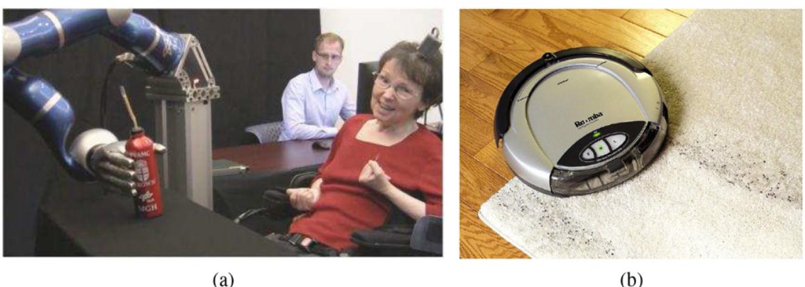
1. A patient with a brain–machine interface controlling a robot arm to grab a drink. Image courtesy of Brown University. (b) Roomba, the robot vacuum cleaner.

Photo by HANDOUT/KRT/Newscom.

Personal robots are meant to assist us with daily tasks like cleaning and organizing, freeing up our time. Although manipulation still has a way to go before it can operate seamlessly in messy, unstructured human environments, navigation has made some headway. In

particular, many homes already enjoy a mobile robot vacuum cleaner like the one in Figure 26.33(b) .

HEALTH CARE: Robots assist and augment surgeons, enabling more precise, minimally invasive, safer procedures with better patient outcomes. The Da Vinci surgical robot from Figure 26.34(a) is now widely deployed at hospitals in the U.S.

Figure 26.34

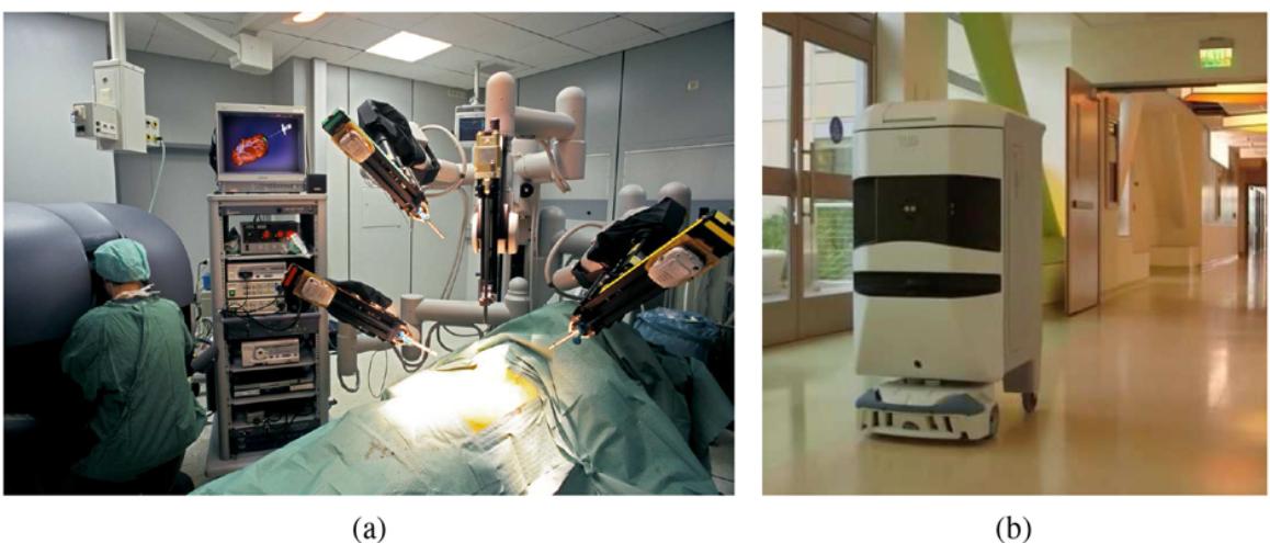
1. Surgical robot in the operating room. Photo by Patrick Landmann/Science Source. (b) Hospital delivery robot. Photo by Wired.

Telepresence robots

SERVICES: Mobile robots help out in office buildings, hotels, and hospitals. Savioke has put robots in hotels delivering products like towels or toothpaste to your room. The Helpmate and TUG robots carry food and medicine in hospitals (Figure 26.34(b) ), while Diligent Robotics’ Moxi robot helps out nurses with back-end logistical responsibilities. Co-Bot roams the halls of Carnegie Mellon University, ready to guide you to someone’s office. We can also use telepresence robots like the Beam to attend meetings and conferences remotely, or check in on our grandparents.

AUTONOMOUS CARS: Some of us are occasionally distracted while driving, by cell phone calls, texts, or other distractions. The sad result: more than a million people die every year in traffic accidents. Further, many of us spend a lot of time driving and would like to recapture some of that time. All this has led to a massive ongoing effort to deploy autonomous cars.

Prototypes have existed since the 1980s, but progress was stimulated by the 2005 DARPA Grand Challenge, an autonomous vehicle race over 200 challenging kilometers of unrehearsed desert terrain. Stanford’s Stanley vehicle completed the course in less than seven hours, winning a $2 million prize and a place in the National Museum of American History. Figure 26.35(a) depicts BOSS, which in 2007 won the DARPA Urban Challenge, a complicated road race on city streets where robots faced other robots and had to obey traffic rules.

Figure 26.35

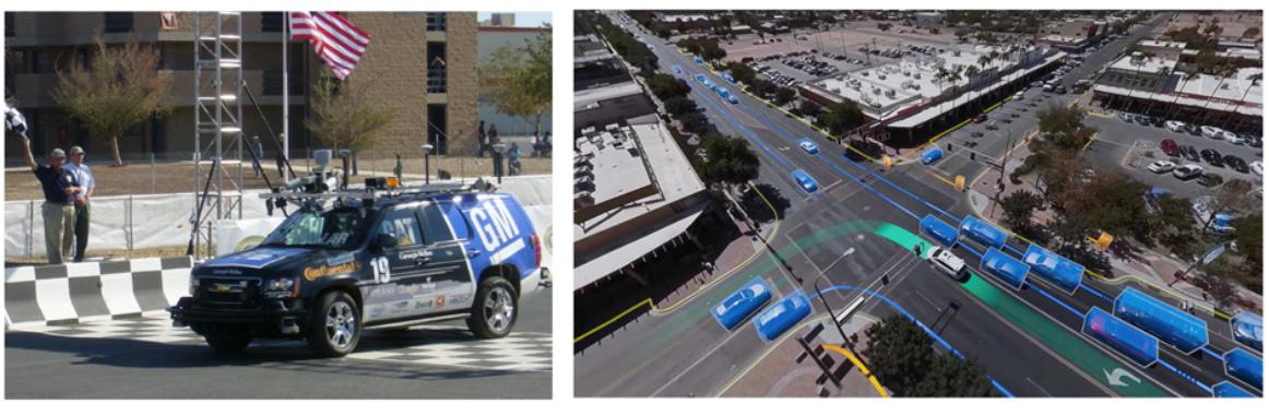
1. Autonomous car BOSS which won the DARPA Urban Challenge. Photo by Tangi Quemener/AFP/Getty Images/Newscom. Courtesy of Sebastian Thrun. (b) Aerial view showing the perception and predictions of the Waymo autonomous car (white vehicle with green track). Other vehicles (blue boxes) and pedestrians (orange boxes) are shown with anticipated trajectories. Road/sidewalk boundaries are in yellow. Photo courtesy of Waymo.

In 2009, Google started an autonomous driving project (featuring many of the researchers who had worked on Stanley and BOSS), which has now spun off as Waymo. In 2018 Waymo started driverless testing (with nobody in the driver seat) in the suburbs of Pheonix, Arizona. In the meantime, other autonomous driving companies and ride-sharing companies are working on developing their own technology, while car manufacturers have been selling cars with more and more assistive intelligence, such as Tesla’s driver assist,

which is meant for highway driving. Other companies are targeting non-highway driving applications including college campuses and retirement communities. Still other companies are focused on non-passenger applications such as trucking, grocery delivery, and valet parking.

Driver assist

ENTERTAINMENT: Disney has been using robots (under the name animatronics) in their parks since 1963. Originally, these robots were restricted to hand-designed, open-loop, unvarying motion (and speech), but since 2009 a version called autonomatronics can generate autonomous actions. Robots also take the form of intelligent toys for children; for example, Anki’s Cozmo plays games with children and may pound the table with frustration when it loses. Finally, quadrotors like Skydio’s R1 from Figure 26.2(b) act as personal photographers and videographers, following us around to take action shots as we ski or bike.

Animatronics

Autonomatronics

EXPLORATION AND HAZARDOUS ENVIRONMENTS: Robots have gone where no human has gone before, including the surface of Mars. Robotic arms assist astronauts in deploying and retrieving satellites and in building the International Space Station. Robots also help explore under the sea. They are routinely used to acquire maps of sunken ships. Figure 26.36 shows a robot mapping an abandoned coal mine, along with a 3D model of the mine acquired using range sensors. In 1996, a team of researches released a legged robot into the crater of an active volcano to acquire data for climate research. Robots are

becoming very effective tools for gathering information in domains that are difficult (or dangerous) for people to access.

Figure 26.36

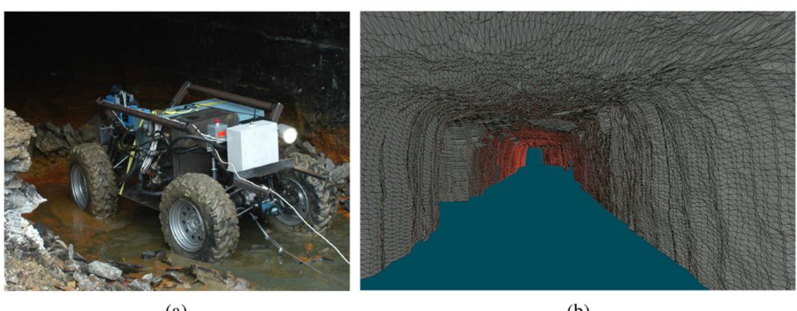
1. A robot mapping an abandoned coal mine. (b) A 3D map of the mine acquired by the robot. Courtesy of Sebastian Thrun.

Robots have assisted people in cleaning up nuclear waste, most notably in Three Mile Island, Chernobyl, and Fukushima. Robots were present after the collapse of the World Trade Center, where they entered structures deemed too dangerous for human search and rescue crews. Here too, these robots are initially deployed via teleoperation, and as technology advances they are becoming more and more autonomous, with a human operator in charge but not having to specify every single command.

INDUSTRY: The majority of robots today are deployed in factories, automating tasks that are difficult, dangerous, or dull for humans. (The majority of factory robots are in automobile factories.) Automating these tasks is a positive in terms of efficiently producing what society needs. At the same time, it also means displacing some human workers from their jobs. This has important policy and economics implications—the need for retraining and education, the need for a fair division of resources, etc. These topics are discussed further in Section 27.3.5 .

Summary

Robotics is about physically embodied agents, which can change the state of the physical world. In this chapter, we have learned the following:

• The most common types of robots are manipulators (robot arms) and mobile robots. They have sensors for perceiving the world and actuators that produce motion, which then affects the world via effectors.
• The general robotics problem involves stochasticity (which can be handled by MDPs), partial observability (which can be handled by POMDPs), and acting with and around other agents (which can be handled with game theory). The problem is made even harder by the fact that most robots work in continuous and high-dimensional state and action spaces. They also operate in the real world, which refuses to run faster than real time and in which failures lead to real things being damaged, with no “undo” capability.
• Ideally, the robot would solve the entire problem in one go: observations in the form of raw sensor feeds go in, and actions in the form of torques or currents to the motors come out. In practice though, this is too daunting, and roboticists typically decouple different aspects of the problem and treat them independently.
• We typically separate perception (estimation) from action (motion generation). Perception in robotics involves computer vision to recognize the surroundings through cameras, but also localization and mapping.
• Robotic perception concerns itself with estimating decision-relevant quantities from sensor data. To do so, we need an internal representation and a method for updating this internal representation over time.
• Probabilistic filtering algorithms such as particle filters and Kalman filters are useful for robot perception. These techniques maintain the belief state, a posterior distribution over state variables.
• For generating motion, we use configuration spaces, where a point specifies everything we need to know to locate every body point on the robot. For instance, for a robot arm with two joints, a configuration consists of the two joint angles.
• We typically decouple the motion generation problem into motion planning, concerned with producing a plan, and trajectory tracking control, concerned with producing a policy for control inputs (actuator commands) that results in executing the plan.
• Motion planning can be solved via graph search using cell decomposition; using randomized motion planning algorithms, which sample milestones in the continuous configuration space; or using trajectory optimization, which can iteratively push a straight-line path out of collision by leveraging a signed distance field.
• A path found by a search algorithm can be executed using the path as the reference trajectory for a PID controller, which constantly corrects for errors between where the robot is and where it is supposed to be, or via computed torque control, which adds a feedforward term that makes use of inverse dynamics to compute roughly what torque to send to make progress along the trajectory.
• Optimal control unites motion planning and trajectory tracking by computing an optimal trajectory directly over control inputs. This is especially easy when we have quadratic costs and linear dynamics, resulting in a linear quadratic regulator (LQR). Popular methods make use of this by linearizing the dynamics and computing secondorder approximations of the cost (ILQR).
• Planning under uncertainty unites perception and action by online replanning (such as model predictive control) and information gathering actions that aid perception.
• Reinforcement learning is applied in robotics, with techniques striving to reduce the required number of interactions with the real world. Such techniques tend to exploit models, be it estimating models and using them to plan, or training policies that are robust with respect to different possible model parameters.
• Interaction with humans requires the ability to coordinate the robot’s actions with theirs, which can be formulated as a game. We usually decompose the solution into prediction, in which we use the person’s ongoing actions to estimate what they will do in the future, and action, in which we use the predictions to compute the optimal motion for the robot.
• Helping humans also requires the ability to learn or infer what they want. Robots can approach this by learning the desired cost function they should optimize from human input, such as demonstrations, corrections, or instruction in natural language. Alternatively, robots can imitate human behavior, and use reinforcement learning to help tackle the challenge of generalization to new states.

Bibliographical and Historical Notes

The word robot was popularized by Czech playwright Karel Čapek in his 1920 play R.U.R. (Rossum’s Universal Robots). The robots, which were grown chemically rather than constructed mechanically, end up resenting their masters and decide to take over. It appears that it was Čapek’s brother, Josef, who first combined the Czech words “robota” (obligatory work) and “robotnik” (serf) to yield “robot” in his 1917 short story Opilec (Glanc, 1978). The term robotics was invented for a science fiction story (Asimov, 1950).

The idea of an autonomous machine predates the word “robot” by thousands of years. In 7th century BCE Greek mythology, a robot named Talos was built by Hephaistos, the Greek god of metallurgy, to protect the island of Crete. The legend is that the sorceress Medea defeated Talos by promising him immortality but then draining his life fluid. Thus, this is the first example of a robot making a mistake in the process of changing its objective function. In 322 BCE, Aristotle anticipated technological unemployment, speculating “If every tool, when ordered, or even of its own accord, could do the work that befits it… then there would be no need either of apprentices for the master workers or of slaves for the lords.”

In the 3rd century BCE an actual humanoid robot called the Servant of Philon could pour wine or water into a cup; a series of valves cut off the flow at the right time. Wonderful automata were built in the 18th century—Jacques Vaucanson’s mechanical duck from 1738 being one early example—but the complex behaviors they exhibited were entirely fixed in advance. Possibly the earliest example of a programmable robot-like device was the Jacquard loom (1805), described on page 15.

Grey Walter’s “turtle,” built in 1948, could be considered the first autonomous mobile robot, although its control system was not programmable. The “Hopkins Beast,” built in 1960 at Johns Hopkins University, was much more sophisticated; it had sonar and photocell sensors, pattern-recognition hardware, and could recognize the cover plate of a standard AC power outlet. It was capable of searching for outlets, plugging itself in, and then recharging its batteries! Still, the Beast had a limited repertoire of skills.

The first general-purpose mobile robot was “Shakey,” developed at what was then the Stanford Research Institute (now SRI) in the late 1960s (Fikes and Nilsson, 1971; Nilsson, 1984). Shakey was the first robot to integrate perception, planning, and execution, and much subsequent research in AI was influenced by this remarkable achievement. Shakey appears on the cover of this book with project leader Charlie Rosen (1917–2002). Other influential projects include the Stanford Cart and the CMU Rover (Moravec, 1983). Cox and Wilfong, (1990) describe classic work on autonomous vehicles.

The first commercial robot was an arm called UNIMATE, for universal automation, developed by Joseph Engelberger and George Devol in their compnay, Unimation. In 1961, the first UNIMATE robot was sold to General Motors for use in manufacturing TV picture tubes. 1961 was also the year when Devol obtained the first U.S. patent on a robot.

In 1973, Toyota and Nissan started using an updated version of UNIMATE for auto body spot welding. This initiated a major revolution in automobile manufacturing that took place mostly in Japan and the U.S., and that is still ongoing. Unimation followed up in 1978 with the development of the Puma robot (Programmable Universal Machine for Assembly), which was the de facto standard for robotic manipulation for the two decades that followed. About 500,000 robots are sold each year, with half of those going to the automotive industry.

In manipulation, the first major effort at creating a hand–eye machine was Heinrich Ernst’s MH-1, described in his MIT Ph.D. thesis (Ernst, 1961). The Machine Intelligence project at Edinburgh also demonstrated an impressive early system for vision-based assembly called FREDDY (Michie, 1972).

Research on mobile robotics has been stimulated by several important competitions. AAAI’s annual mobile robot competition began in 1992. The first competition winner was CARMEL (Congdon et al., 1992). Progress has been steady and impressive: in recent competitions robots entered the conference complex, found their way to the registration desk, registered for the conference, and even gave a short talk.

The RoboCup competition, launched in 1995 by Kitano and colleagues (1997), aims to “develop a team of fully autonomous humanoid robots that can win against the human world champion team in soccer” by 2050. Some competitions use wheeled robots, some humanoid robots, and some software simulations. Stone, (2016) describes recent innovations in RoboCup.

The DARPA Grand Challenge, organized by DARPA in 2004 and 2005, required autonomous vehicles to travel more than 200 kilometers through the desert in less than ten hours (Buehler et al., 2006). In the original event in 2004, no robot traveled more than eight miles, leading many to believe the prize would never be claimed. In 2005, Stanford’s robot Stanley won the competition in just under seven hours (Thrun, 2006). DARPA then organized the Urban Challenge, a competition in which robots had to navigate 60 miles in an urban environment with other traffic. Carnegie Mellon University’s robot BOSS took first place and claimed the $2 million prize (Urmson and Whittaker, 2008). Early pioneers in the development of robotic cars included Dickmanns and Zapp, (1987) and Pomerleau, (1993).

The field of robotic mapping has evolved from two distinct origins. The first thread began with work by Smith and Cheeseman (1986), who applied Kalman filters to the simultaneous localization and mapping (SLAM) problem. This algorithm was first implemented by Moutarlier and Chatila (1989), and later extended by Leonard and Durrant-Whyte, (1992); see Dissanayake et al., (2001) for an overview of early Kalman filter variations. The second thread began with the development of the occupancy grid representation for probabilistic mapping, which specifies the probability that each location is occupied by an obstacle (Moravec and Elfes, 1985).

Occupancy grid

Kuipers and Levitt, (1988) were among the first to propose topological rather than metric mapping, motivated by models of human spatial cognition. A seminal paper by Lu and Milios, (1997) recognized the sparseness of the simultaneous localization and mapping problem, which gave rise to the development of nonlinear optimization techniques by Konolige, (2004) and Montemerlo and Thrun, (2004), as well as hierarchical methods by Bosse et al., (2004). Shatkay and Kaelbling, (1997) and Thrun et al., (1998) introduced the EM algorithm into the field of robotic mapping for data association. An overview of probabilistic mapping methods can be found in (Thrun et al., 2005).

Early mobile robot localization techniques are surveyed by Borenstein et al., (1996). Although Kalman filtering was well known as a localization method in control theory for decades, the general probabilistic formulation of the localization problem did not appear in the AI literature until much later, through the work of Tom Dean and colleagues (Dean et al., 1990) and of Simmons and Koenig, (1995). The latter work introduced the term Markov localization. The first real-world application of this technique was by Burgard et al., (1999), through a series of robots that were deployed in museums. Monte Carlo localization based on particle filters was developed by Fox et al., (1999) and is now widely used. The Rao-Blackwellized particle filter combines particle filtering for robot localization with exact filtering for map building (Murphy and Russell, 2001; Montemerlo et al., 2002).

Markov localization

Rao-Blackwellized particle filter

A great deal of early work on motion planning focused on geometric algorithms for deterministic and fully observable motion planning problems. The PSPACE-hardness of robot motion planning was shown in a seminal paper by Reif (1979). The configuration space representation is due to Lozano-Perez, (1983). A series of papers by Schwartz and Sharir on what they called piano movers problems (Schwartz et al., 1987) was highly influential.

Piano movers

Recursive cell decomposition for configuration space planning was originated in the work of Brooks and Lozano-Perez, (1985) and improved significantly by Zhu and Latombe, (1991). The earliest skeletonization algorithms were based on Voronoi diagrams (Rowat, 1979) and visibility graphs (Wesley and Lozano-Perez, 1979). Guibas et al., (1992) developed efficient

techniques for calculating Voronoi diagrams incrementally, and Choset, (1996) generalized Voronoi diagrams to broader motion planning problems.

Visibility graph

John Canny (1988) established the first singly exponential algorithm for motion planning. The seminal text by Latombe (1991) covers a variety of approaches to motion planning, as do the texts by Choset et al., (2005) and LaValle, (2006). Kavraki et al., (1996) developed the theory of probabilistic roadmaps. Kuffner and LaValle, (2000) developed rapidly exploring random trees (RRTs).

Involving optimization in geometric motion planning began with elastic bands (Quinlan and Khatib, 1993), which refine paths when the configuration-space obstacles change. Ratliff et al., (2009) formulated the idea as the solution to an optimal control problem, allowing the initial trajectory to start in collision, and deforming it by mapping workspace obstacle gradients via the Jacobian into the configuration space. Schulman et al., (2013) proposed a practical second-order alternative.

The control of robots as dynamical systems—whether for manipulation or navigation—has generated a vast literature. While this chapter explained the basics of trajectory tracking control and optimal control, it left out entire subfields, including adaptive control, robust control, and Lyapunov analysis. Rather than assuming everything about the system is known a priori, adaptive control aims to adapt the dynamics parameters and/or the control law online. Robust control, on the other hand, aims to design controllers that perform well in spite of uncertainty and external disturbances.

Lyapunov analysis was originally developed in the 1890s for the stability analysis of general nonlinear systems, but it was not until the early 1930s that control theorists realized its true potential. With the development of optimization methods, Lyapunov analysis was extended to control barrier functions, which lend themselves nicely to modern optimization tools. These methods are widely used in modern robotics for real-time controller design and safety analysis.

Crucial works in robotic control include a trilogy on impedance control by Hogan (1985), and a general study of robot dynamics by Featherstone, (1987). Dean and Wellman, (1991) were among the first to try to tie together control theory and AI planning systems. Three classic textbooks on the mathematics of robot manipulation are due to Paul (1981), Craig (1989), and Yoshikawa (1990). Control for manipulation is covered by Murray, (2017).

The area of grasping is also important in robotics—the problem of determining a stable grasp is quite difficult (Mason and Salisbury, 1985). Competent grasping requires touch sensing, or haptic feedback, to determine contact forces and detect slip (Fearing and Hollerbach, 1985). Understanding how to grasp the the wide variety of objects in the world is a daunting task. (Bousmalis et al., 2017) describe a system that combines real-world experimentation with simulations guided by sim-to-real transfer to produce robust grasping.

Haptic feedback

Potential-field control, which attempts to solve the motion planning and control problems simultaneously, was developed for robotics by Khatib (1986). In mobile robotics, this idea was viewed as a practical solution to the collision avoidance problem, and was later extended into an algorithm called vector field histograms by Borenstein (1991).

Vector field histogram

ILQR is currently widely used at the intersection of motion planning and control and is due to Li and Todorov, (2004). It is a variant of the much older differential dynamic programming technique (Jacobson and Mayne, 1970).

Fine-motion planning with limited sensing was investigated by Lozano-Perez et al., (1984) and Canny and Reif, (1987). Landmark-based navigation (Lazanas and Latombe, 1992) uses many of the same ideas in the mobile robot arena. Navigation functions, the robotics

version of a control policy for deterministic MDPs, were introduced by Koditschek, (1987). Key work applying POMDP methods (Section 17.4 ) to motion planning under uncertainty in robotics is due to Pineau et al., (2003) and Roy et al., (2005).

Reinforcement learning in robotics took off with the seminal work by Bagnell and Schneider, (2001) and Ng et al., (2003), who developed the paradigm in the context of autonomous helicopter control. Kober et al., (2013) offers an overview of how reinforcement learning changes when applied to the robotics problem. Many of the techniques implemented on physical systems build approximate dynamics models, dating back to locally weighted linear models due to Atkeson et al., (1997). But policy gradients played their role as well, enabling (simplified) humanoid robots to walk (Tedrake et al., 2004), or a robot arm to hit a baseball (Peters and Schaal, 2008).

Levine et al., (2016) demonstrated the first deep reinforcement learning application on a real robot. At the same time, model-free RL in simulation was being extended to continuous domains (Schulman et al., 2015a; Heess et al., 2016; Lillicrap et al., 2015). Other work scaled up physical data collection massively to showcase the learning of grasps and dynamics models (Pinto and Gupta, 2016; Agrawal et al., 2017; Levine et al., 2018). Transfer from simulation to reality or sim-to-real (Sadeghi and Levine, 2016; Andrychowicz et al., 2018a), metalearning (Finn et al., 2017), and sample-efficient model-free reinforcement learning (Andrychowicz et al., 2018b) are active areas of research.

Early methods for predicting human actions made use of filtering approaches (Madhavan and Schlenoff, 2003), but seminal work by Ziebart et al., (2009) proposed prediction by modeling people as approximately rational agents. Sadigh et al., (2016) captured how these predictions should actually depend on what the robot decides to do, building toward a game-theoretic setting. For collaborative settings, Sisbot et al., (2007) pioneered the idea of accounting for what people want in the robot’s cost function. Nikolaidis and Shah, (2013) decomposed collaboration into learning how the human will act, but also learning how the human wants the robot to act, both achievable from demonstrations. For learning from demonstration see Argall et al., (2009). Akgun et al., (2012) and Sefidgar et al., (2017) studied teaching by end users rather than by experts.

Tellex et al., (2011) showed how robots can infer what people want from natural language instructions. Finally, not only do robots need to infer what people want and plan on doing, but people too need to make the same inferences about robots. Dragan et al., (2013) incorporated a model of the human’s inferences into robot motion planning.

The field of human–robot interaction is much broader than what we covered in this chapter, which focused primarily on the planning and learning aspects. Thomaz et al., (2016) provides a survey of interaction more broadly from a computational perspective. Ross et al., (2011) describe the DAGGER system.

The topic of software architectures for robots engenders much religious debate. The good old-fashioned AI candidate—the three-layer architecture—dates back to the design of Shakey and is reviewed by Gat (1998). The subsumption architecture is due to Brooks (1986), although similar ideas were developed independently by Braitenberg, whose book, Vehicles (1984), describes a series of simple robots based on the behavioral approach.

The success of Brooks’s six-legged walking robot was followed by many other projects. Connell, in his Ph.D. thesis (1989), developed an entirely reactive mobile robot that was capable of retrieving objects. Extensions of the paradigm to multirobot systems can be found in work by Parker (1996) and Mataric (1997). GRL (Horswill, 2000) and COLBERT (Konolige, 1997) abstract the ideas of concurrent behavior-based robotics into general robot control languages. Arkin (1998) surveys some of the most popular approaches in this field.

Two early textbooks, by Dudek and Jenkin (2000) and by Murphy (2000), cover robotics generally. More recent overviews are due to Bekey (2008) and Lynch and Park (2017). An excellent book on robot manipulation addresses advanced topics such as compliant motion (Mason 2001). Robot motion planning is covered in Choset et al., (2005) and LaValle, (2006). Thrun et al., (2005) introduces probabilistic robotics. The Handbook of Robotics (Siciliano and Khatib, 2016) is a massive, comprehensive overview of all of robotics.

The premiere conference for robotics is Robotics: Science and Systems Conference, followed by the IEEE International Conference on Robotics and Automation. Human–Robot Interaction is the premiere venue for interaction. Leading robotics journals include IEEE Robotics and Automation, the International Journal of Robotics Research, and Robotics and Autonomous Systems.

VII Conclusions

Chapter 27 Philosophy, Ethics, and Safety of AI

In which we consider the big questions around the meaning of AI, how we can ethically develop and apply it, and how we can keep it safe.

Philosophers have been asking big questions for a long time: How do minds work? Is it possible for machines to act intelligently in the way that people do? Would such machines have real, conscious minds?

To these, we add new ones: What are the ethical implications of intelligent machines in dayto-day use? Should machines be allowed to decide to kill humans? Can algorithms be fair and unbiased? What will humans do if machines can do all kinds of work? And how do we control machines that may become more intelligent than us?

27.1 The Limits of AI

In 1980, philosopher John Searle introduced a distinction between weak AI—the idea that machines could act as if they were intelligent—and strong AI—the assertion that machines that do so are actually consciously thinking (not just simulating thinking). Over time the definition of strong AI shifted to refer to what is also called “human-level AI” or “general AI”—programs that can solve an arbitrarily wide variety of tasks, including novel ones, and do so as well as a human.

Weak AI

Strong AI

Critics of weak AI who objected to the very possibility of intelligent behavior in machines now appear as shortsighted as Simon Newcomb, who in October 1903 wrote “aerial flight is one of the great class of problems with which man can never cope”—just two months before the Wright brothers’ flight at Kitty Hawk. The rapid progress of recent years does not, however, prove that there can be no limits to what AI can achieve. Alan Turing (1950), the first person to define AI, was also the first to raise possible objections to AI, foreseeing almost all the ones subsequently raised by others.

27.1.1 The argument from informality

Turing’s “argument from informality of behavior” says that human behavior is far too complex to be captured by any formal set of rules—humans must be using some informal guidelines that (the argument claims) could never be captured in a formal set of rules and thus could never be codified in a computer program.

A key proponent of this view was Hubert Dreyfus, who produced a series of influential critiques of artificial intelligence: What Computers Can’t Do (1972), the sequel What Computers Still Can’t Do (1992), and, with his brother Stuart, Mind Over Machine (1986). Similarly, philosopher Kenneth Sayre (1993) said “Artificial intelligence pursued within the cult of computationalism stands not even a ghost of a chance of producing durable results.” The technology they criticize came to be called Good Old-Fashioned AI (GOFAI).

Good Old-Fashioned AI (GOFAI)

GOFAI corresponds to the simplest logical agent design described in Chapter 7 , and we saw there that it is indeed difficult to capture every contingency of appropriate behavior in a set of necessary and sufficient logical rules; we called that the qualification problem. But as we saw in Chapter 12 , probabilistic reasoning systems are more appropriate for openended domains, and as we saw in Chapter 21 , deep learning systems do well on a variety of “informal” tasks. Thus, the critique is not addressed against computers per se, but rather against one particular style of programming them with logical rules—a style that was popular in the 1980s but has been eclipsed by new approaches.

One of Dreyfus’s strongest arguments is for situated agents rather than disembodied logical inference engines. An agent whose understanding of “dog” comes only from a limited set of logical sentences such as ” ” is at a disadvantage compared to an agent that has watched dogs run, has played fetch with them, and has been licked by one. As philosopher Andy Clark (1998) says, “Biological brains are first and foremost the control systems for biological bodies. Biological bodies move and act in rich real-world surroundings.” According to Clark, we are “good at frisbee, bad at logic.”

The embodied cognition approach claims that it makes no sense to consider the brain separately: cognition takes place within a body, which is embedded in an environment. We need to study the system as a whole; the brain’s functioning exploits regularities in its environment, including the rest of its body. Under the embodied cognition approach, robotics, vision, and other sensors become central, not peripheral.

Embodied cognition

Overall, Dreyfus saw areas where AI did not have complete answers and said that AI is therefore impossible; we now see many of these same areas undergoing continued research and development leading to increased capability, not impossibility.

27.1.2 The argument from disability

The “argument from disability” makes the claim that “a machine can never do .” As examples of , Turing lists the following:

Be kind, resourceful, beautiful, friendly, have initiative, have a sense of humor, tell right from wrong, make mistakes, fall in love, enjoy strawberries and cream, make someone fall in love with it, learn from experience, use words properly, be the subject of its own thought, have as much diversity of behavior as man, do something really new.

In retrospect, some of these are rather easy—we’re all familiar with computers that “make mistakes.” Computers with metareasoning capabilities (Chapter 5 ) can examine heir own computations, thus being the subject of their own reasoning. A century-old technology has the proven ability to “make someone fall in love with it”—the teddy bear. Computer chess expert David Levy predicts that by 2050 people will routinely fall in love with humanoid robots. As for a robot falling in love, that is a common theme in fiction, but there has been only limited academic speculation on the subject (Kim et al., 2007). Computers have done things that are “really new,” making significant discoveries in astronomy, mathematics, chemistry, mineralogy, biology, computer science, and other fields, and creating new forms of art through style transfer (Gatys et al., 2016). Overall, programs exceed human performance in some tasks and lag behind on others. The one thing that it is clear they can’t do is be exactly human. 1

1 For example, the opera Coppélia (1870), the novel Do Androids Dream of Electric Sheep? (1968), the movies AI (2001), Wall-E (2008), and Her (2013).

27.1.3 The mathematical objection

Turing (1936) and Gödel (1931) proved that certain mathematical questions are in principle unanswerable by particular formal systems. Gödel’s incompleteness theorem (see Section 9.5 ) is the most famous example of this. Briefly, for any formal axiomatic framework powerful enough to do arithmetic, it is possible to construct a so-called Gödel sentence with the following properties:

• is a sentence of , but cannot be proved within .
• If is consistent, then is true.

Philosophers such as J. R. Lucas (1961) have claimed that this theorem shows that machines are mentally inferior to humans, because machines are formal systems that are limited by the incompleteness theorem—they cannot establish the truth of their own Gödel sentence while humans have no such limitation. This has caused a lot of controversy, spawning a vast literature, including two books by the mathematician/physicist Sir Roger Penrose (1989, 1994). Penrose repeats Lucas’s claim with some fresh twists, such as the hypothesis that humans are different because their brains operate by quantum gravity—a theory that makes multiple false predictions about brain physiology.

We will examine three of the problems with Lucas’s claim. First, an agent should not be ashamed that it cannot establish the truth of some sentence while other agents can. Consider the following sentence:

Lucas cannot consistently assert that this sentence is true.

If Lucas asserted this sentence, then he would be contradicting himself, so therefore Lucas cannot consistently assert it, and hence it is true. We have thus demonstrated that there is a true sentence that Lucas cannot consistently assert while other people (and machines) can. But that does not make us think any less of Lucas.

Second, Gödel’s incompleteness theorem and related results apply to mathematics, not to computers. No entity—human or machine—can prove things that are impossible to prove. Lucas and Penrose falsely assume that humans can somehow get around these limits, as when Lucas (1976) says “we must assume our own consistency, if thought is to be possible at all.” But this is an unwarranted assumption: humans are notoriously inconsistent. This is certainly true for everyday reasoning, but it is also true for careful mathematical thought. A famous example is the four-color map problem. Alfred Kempe (1879) published a proof that was widely accepted for 11 years until Percy Heawood (1890) pointed out a flaw.

Third, Gödel’s incompleteness theorem technically applies only to formal systems that are powerful enough to do arithmetic. This includes Turing machines, and Lucas’s claim is in part based on the assertion that computers are equivalent to Turing machines. This is not quite true. Turing machines are infinite, whereas computers (and brains) are finite, and any computer can therefore be described as a (very large) system in propositional logic, which is not subject to Gödel’s incompleteness theorem. Lucas assumes that humans can “change their minds” while computers cannot, but that is also false—a computer can retract a conclusion after new evidence or further deliberation; it can upgrade its hardware; and it can change its decision-making processes with machine learning or software rewriting.

27.1.4 Measuring AI

Alan Turing, in his famous paper “Computing Machinery and Intelligence” (1950), suggested that instead of asking whether machines can think, we should ask whether machines can pass a behavioral test, which has come to be called the Turing test. The test requires a program to have a conversation (via typed messages) with an interrogator for five minutes. The interrogator then has to guess if the conversation is with a program or a person; the program passes the test if it fools the interrogator 30% of the time. To Turing, the key point was not the exact details of the test, but instead the idea of measuring intelligence by performance on some kind of open-ended behavioral task, rather than by philosophical speculation.

Nevertheless, Turing conjectured that by the year 2000 a computer with a storage of a billion units could pass the test, but here we are on the other side of 2000, and we still can’t agree whether any program has passed. Many people have been fooled when they didn’t know they might be chatting with a computer. The ELIZA program and Internet chatbots such as MGONZ (Humphrys, 2008) and NATACHATA (Jonathan et al., 2009) fool their correspondents repeatedly, and the chatbot CYBERLOVER has attracted the attention of law enforcement because of its penchant for tricking fellow chatters into divulging enough personal information that their identity can be stolen.

In 2014, a chatbot called Eugene Goostman fooled 33% of the untrained amateur judges in a Turing test. The program claimed to be a boy from Ukraine with limited command of

English; this helped explain its grammatical errors. Perhaps the Turing test is really a test of human gullibility. So far no well-trained judge has been fooled (Aaronson, 2014).

Turing test competitions have led to better chatbots, but have not been a focus of research within the AI community. Instead, AI researchers who crave competition are more likely to concentrate on playing chess or Go or StarCraft II, or taking an 8th grade science exam, or identifying objects in images. In many of these competitions, programs have reached or surpassed human-level performance, but that doesn’t mean the programs are human-like outside the specific task. The point is to improve basic science and technology and to provide useful tools, not to fool judges.

27.2 Can Machines Really Think?

Some philosophers claim that a machine that acts intelligently would not be actually thinking, but would be only a simulation of thinking. But most AI researchers are not concerned with the distinction, and the computer scientist Edsger Dijkstra (1984) said that “The question of whether Machines Can Think … is about as relevant as the question of whether Submarines Can Swim.” The American Heritage Dictionary’s first definition of swim is “To move through water by means of the limbs, fins, or tail,” and most people agree that submarines, being limbless, cannot swim. The dictionary also defines fly as “To move through the air by means of wings or winglike parts,” and most people agree that airplanes, having winglike parts, can fly. However, neither the questions nor the answers have any relevance to the design or capabilities of airplanes and submarines; rather they are about word usage in English. (The fact that ships do swim ( “privet”) in Russian amplifies this point.) English speakers have not yet settled on a precise definition for the word “think” does it require “a brain” or just “brain-like parts?”

Again, the issue was addressed by Turing. He notes that we never have any direct evidence about the internal mental states of other humans—a kind of mental solipsism. Nevertheless, Turing says, “Instead of arguing continually over this point, it is usual to have the polite convention that everyone thinks.” Turing argues that we would also extend the polite convention to machines, if only we had experience with ones that act intelligently. However, now that we do have some experience, it seems that our willingness to ascribe sentience depends at least as much on humanoid appearance and voice as on pure intelligence.

Polite convention

27.2.1 The Chinese room

The philosopher John Searle rejects the polite convention. His famous Chinese room argument (Searle, 1990) goes as follows: Imagine a human, who understands only English, inside a room that contains a rule book, written in English, and various stacks of paper. Pieces of paper containing indecipherable symbols are slipped under the door to the room. The human follows the instructions in the rule book, finding symbols in the stacks, writing symbols on new pieces of paper, rearranging the stacks, and so on. Eventually, the instructions will cause one or more symbols to be transcribed onto a piece of paper that is passed back to the outside world. From the outside, we see a system that is taking input in the form of Chinese sentences and generating fluent, intelligent Chinese responses.

Chinese room

Searle then argues: it is given that the human does not understand Chinese. The rule book and the stacks of paper, being just pieces of paper, do not understand Chinese. Therefore, there is no understanding of Chinese. And Searle says that the Chinese room is doing the same thing that a computer would do, so therefore computers generate no understanding.

Searle (1980) is a proponent of biological naturalism, according to which mental states are high-level emergent features that are caused by low-level physical processes in the neurons, and it is the (unspecified) properties of the neurons that matter: according to Searle’s biases, neurons have “it” and transistors do not. There have been many refutations of Searle’s argument, but no consensus. His argument could equally well be used (perhaps by robots) to argue that a human cannot have true understanding; after all, a human is made out of cells, the cells do not understand, therefore there is no understanding. In fact, that is the plot of Terry Bisson’s (1990) science fiction story They’re Made Out of Meat, in which alien robots explore Earth and can’t believe that hunks of meat could possibly be sentient. How they can be remains a mystery.

Biological naturalism

27.2.2 Consciousness and qualia

Running through all the debates about strong AI is the issue of consciousness: awareness of the outside world, and of the self, and the subjective experience of living. The technical term for the intrinsic nature of experiences is qualia (from the Latin word meaning, roughly, “of what kind”). The big question is whether machines can have qualia. In the movie 2001, when astronaut David Bowman is disconnecting the “cognitive circuits” of the HAL 9000 computer, it says “I’m afraid, Dave. Dave, my mind is going. I can feel it.” Does HAL actually have feelings (and deserve sympathy)? Or is the reply just an algorithmic response, no different from “Error 404: not found”?

Consciousness

Qualia

There is a similar question for animals: pet owners are certain that their dog or cat has consciousness, but not all scientists agree. Crickets change their behavior based on temperature, but few people would say that crickets experience the feeling of being warm or cold.

One reason that the problem of consciousness is hard is that it remains ill-defined, even after centuries of debate. But help may be on the way. Recently philosophers have teamed with neuroscientists under the auspices of the Templeton Foundation to start a series of experiments that could resolve some of the issues. Advocates of two leading theories of consciousness (global workspace theory and integrated information theory) have agreed that the experiments could confirm one theory over the other—a rarity in philosophy.

Alan Turing (1950) concedes that the question of consciousness is a difficult one, but denies that it has much relevance to the practice of AI: “I do not wish to give the impression that I think there is no mystery about consciousness But I do not think these mysteries necessarily need to be solved before we can answer the question with which we are concerned in this paper.” We agree with Turing—we are interested in creating programs that behave intelligently. Individual aspects of consciousness—awareness, self-awareness, attention—can be programmed and can be part of an intelligent machine. The additional project of making a machine conscious in exactly the way humans are is not one that we are equipped to take on. We do agree that behaving intelligently will require some degree of awareness, which will differ from task to task, and that tasks involving interaction with humans will require a model of human subjective experience.

In the matter of modeling experience, humans have a clear advantage over machines, because they can use their own subjective apparatus to appreciate the subjective experience of others. For example, if you want to know what it’s like when someone hits their thumb with a hammer, you can hit your thumb with a hammer. Machines have no such capability although unlike humans, they can run each other’s code.

27.3 The Ethics of AI

Given that AI is a powerful technology, we have a moral obligation to use it well, to promote the positive aspects and avoid or mitigate the negative ones.

The positive aspects are many. For example, AI can save lives through improved medical diagnosis, new medical discoveries, better prediction of extreme weather events, and safer driving with driver assistance and (eventually) self-driving technologies. There are also many opportunities to improve lives. Microsoft’s AI for Humanitarian Action program applies AI to recovering from natural disasters, addressing the needs of children, protecting refugees, and promoting human rights. Google’s AI for Social Good program supports work on rainforest protection, human rights jurisprudence, pollution monitoring, measurement of fossil fuel emissions, crisis counseling, news fact checking, suicide prevention, recycling, and other issues. The University of Chicago’s Center for Data Science for Social Good applies machine learning to problems in criminal justice, economic development, education, public health, energy, and environment.

AI applications in crop management and food production help feed the world. Optimization of business processes using machine learning will make businesses more productive, increasing wealth and providing more employment. Automation can replace the tedious and dangerous tasks that many workers face, and free them to concentrate on more interesting aspects. People with disabilities will benefit from AI-based assistance in seeing, hearing, and mobility. Machine translation already allows people from different cultures to communicate. Software-based AI solutions have near zero marginal cost of production, and so have the potential to democratize access to advanced technology (even as other aspects of software have the potential to centralize power).

Despite these many positive aspects, we shouldn’t ignore the negatives. Many new technologies have had unintended negative side effects: nuclear fission brought Chernobyl and the threat of global destruction; the internal combustion engine brought air pollution, global warming, and the paving of paradise. Other technologies can have negative effects even when used as intended, such as sarin gas, AR-15 rifles, and telephone solicitation. Automation will create wealth, but under current economic conditions much of that wealth will flow to the owners of the automated systems, leading to increased income inequality.

This can be disruptive to a well-functioning society. In developing countries, the traditional path to growth through low-cost manufacturing for export may be cut off, as wealthy countries adopt fully automated manufacturing facilities on-shore. Our ethical and governance decisions will dictate the level of inequality that AI will engender.

Negative side effects

All scientists and engineers face ethical considerations of what projects they should or should not take on, and how they can make sure the execution of the project is safe and beneficial. In 2010, the UK’s Engineering and Physical Sciences Research Council held a meeting to develop a set of Principles of Robotics. In subsequent years other government agencies, nonprofit organizations, and companies created similar sets of principles. The gist is that every organization that creates AI technology, and everyone in the organization, has a responsibility to make sure the technology contributes to good, not harm. The most commonly-cited principles are:

Ensure safety	Establish accountability
Ensure fairness	Uphold human rights and values
Respect privacy	Reflect diversity/inclusion
Promote collaboration	Avoid concentration of power
Provide transparency	Acknowledge legal/policy implications
Limit harmful uses of AI	Contemplate implications for employment

Note that many of the principles, such as “ensure safety,” have applicability to all software or hardware systems, not just AI systems. Several principles are worded in a vague way, making them difficult to measure or enforce. That is in part because AI is a big field with many subfields, each of which has a different set of historical norms and different relationships between the AI developers and the stakeholders. Mittelstadt (2019) suggests that the subfields should each develop more specific actionable guidelines and case precedents.

27.3.1 Lethal autonomous weapons

The UN defines a lethal autonomous weapon as one that locates, selects, and engages (i.e., kills) human targets without human supervision. Various weapons fulfill some of these criteria. For example, land mines have been used since the 17th century: they can select and engage targets in a limited sense according to the degree of pressure exerted or the quantity of metal present, but they cannot go out and locate targets by themselves. (Land mines are banned under the Ottawa Treaty.) Guided missiles, in use since the 1940s, can chase targets, but they have to be pointed in the right general direction by a human. Auto-firing radarcontrolled guns have been used to defend naval ships since the 1970s; they are mainly intended to destroy incoming missiles, but they could also attack manned aircraft. Although the word “autonomous” is often used to describe unmanned air vehicles or drones, most such weapons are both remotely piloted and require human actuation of the lethal payload.

At the time of writing, several weapons systems seem to have crossed the line into full autonomy. For example Israel’s Harop missile is a “loitering munition” with a ten-foot wingspan and a fifty-pound warhead. It searches for up to six hours in a given geographical region for any target that meets a given criterion and then destroys it. The criterion could be “emits a radar signal resembling antiaircraft radar” or “looks like a tank.” The Turkish manufacturer STM advertises its Kargu quadcopter—which carries up to 1.5kg of explosives —as capable of “Autonomous hit … targets selected on images … tracking moving targets … anti-personnel … face recognition.”

Autonomous weapons have been called the “third revolution in warfare” after gunpowder and nuclear weapons. Their military potential is obvious. For example, few experts doubt that autonomous fighter aircraft would defeat any human pilot. Autonomous aircraft, tanks, and submarines can be cheaper, faster, more maneuverable, and have longer range than their manned counterparts.

Since 2014, the United Nations in Geneva has conducted regular discussions under the auspices of the Convention on Certain Conventional Weapons (CCW) on the question of whether to ban lethal autonomous weapons. At the time of writing, 30 nations, ranging in size from China to the Holy See, have declared their support for an international treaty, while other key countries—including Israel, Russia, South Korea, and the United States—are opposed to a ban.

The debate over autonomous weapons includes legal, ethical and practical aspects. The legal issues are governed primarily by the CCW, which requires the possibility of discriminating between combatants and non-combatants, the judgment of military necessity for an attack, and the assessment of proportionality between the military value of a target and the possibility of collateral damage. The feasibility of meeting these criteria is an engineering question—one whose answer will undoubtedly change over time. At present, discrimination seems feasible in some circumstances and will undoubtedly improve rapidly, but necessity and proportionality are not presently feasible: they require that machines make subjective and situational judgments that are considerably more difficult than the relatively simple tasks of searching for and engaging potential targets. For these reasons, it would be legal to use autonomous weapons only in circumstances where a human operator can reasonably predict that the execution of the mission will not result in civilians being targeted or the weapons conducting unnecessary or disproportionate attacks. This means that, for the time being, only very restricted missions could be undertaken by autonomous weapons.

On the ethical side, some find it simply morally unacceptable to delegate the decision to kill humans to a machine. For example, Germany’s ambassador in Geneva has stated that it “will not accept that the decision over life and death is taken solely by an autonomous system” while Japan “has no plan to develop robots with humans out of the loop, which may be capable of committing murder.” Gen. Paul Selva, at the time the second-ranking military officer in the United States, said in 2017, “I don’t think it’s reasonable for us to put robots in charge of whether or not we take a human life.” Finally, António Guterres, the head of the United Nations, stated in 2019 that “machines with the power and discretion to take lives without human involvement are politically unacceptable, morally repugnant and should be prohibited by international law.”

More than 140 NGOs in over 60 countries are part of the Campaign to Stop Killer Robots, and an open letter organized in 2015 by the Future of Life Institute organized an open letter was signed by over 4,000 AI researchers and 22,000 others. 2

2 Including the two authors of this book.

Against this, it can be argued that as technology improves it ought to be possible to develop weapons that are less likely than human soldiers or pilots to cause civilian casualties. (There is also the important benefit that autonomous weapons reduce the need for human soldiers

and pilots to risk death.) Autonomous systems will not succumb to fatigue, frustration, hysteria, fear, anger, or revenge, and need not “shoot first, ask questions later” (Arkin, 2015). Just as guided munitions have reduced collateral damage compared to unguided bombs, one may expect intelligent weapons to further improve the precision of attacks. (Against this, see Benjamin (2013) for an analysis of drone warfare casualties.) This, apparently, is the position of the United States in the latest round of negotiations in Geneva.

Perhaps counterintuitively, the United States is also one of the few nations whose own policies currently preclude the use of autonomous weapons. The 2011 U.S. Department of Defense (DOD) roadmap says: “For the foreseeable future, decisions over the use of force [by autonomous systems] and the choice of which individual targets to engage with lethal force will be retained under human control.” The primary reason for this policy is practical: autonomous systems are not reliable enough to be trusted with military decisions.

The issue of reliability came to the fore on September 26, 1983, when Soviet missile officer Stanislav Petrov’s computer display flashed an alert of an incoming missile attack. According to protocol, Petrov should have initiated a nuclear counterattack, but he suspected the alert was a bug and treated it as such. He was correct, and World War III was (narrowly) averted. We don’t know what would have happened if there had been no human in the loop.

Reliability is a very serious concern for military commanders, who know well the complexity of battlefield situations. Machine learning systems that operate flawlessly in training may perform poorly when deployed. Cyberattacks against autonomous weapons could result in friendly-fire casualties; disconnecting the weapon from all communication may prevent that (assuming it has not already been compromised), but then the weapon cannot be recalled if it is malfunctioning.

The overriding practical issue with autonomous weapons is that they they are scalable weapons of mass destruction, in the sense that the scale of an attack that can be launched is proportional to the amount of hardware one can afford to deploy. A quadcopter two inches in diameter can carry a lethal explosive charge, and one million can fit in a regular shipping container. Precisely because they are autonomous, these weapons would not need one million human supervisors to do their work.

As weapons of mass destruction, scalable autonomous weapons have advantages for the attacker compared to nuclear weapons and carpet bombing: they leave property intact and can be applied selectively to eliminate only those who might threaten an occupying force. They could certainly be used to wipe out an entire ethnic group or all the adherents of a particular religion. In many situations, they would also be untraceable. These characteristics make them particularly attractive to non-state actors.

These considerations—particularly those characteristics that advantage the attacker—suggest that autonomous weapons will reduce global and national security for all parties. The rational response for governments seems to be to engage in arms control discussions rather than an arms race.

The process of designing a treaty is not without its difficulties, however. AI is a dual use technology: AI technologies that have peaceful applications such as flight control, visual tracking, mapping, navigation, and multiagent planning, can easily be applied to military purposes. It is easy to turn an autonomous quadcopter into a weapon simply by attaching an explosive and commanding it to seek out a target. Dealing with this will require careful implementation of compliance regimes with industry cooperation, as has already been demonstrated with some success by the Chemical Weapons Convention.

Dual use

27.3.2 Surveillance, security, and privacy

In 1976, Joseph Weizenbaum warned that automated speech recognition technology could lead to widespread wiretapping, and hence to a loss of civil liberties. Today, that threat has been realized, with most electronic communication going through central servers that can be monitored, and cities packed with microphones and cameras that can identify and track individuals based on their voice, face, and gait. Surveillance that used to require expensive and scarce human resources can now be done at a mass scale by machines.

As of 2018, there were as many as 350 million surveillance cameras in China and 70 million in the United States. China and other countries have begun exporting surveillance

technology to low-tech countries, some with reputations for mistreating their citizens and disproportionately targeting marginalized communities. AI engineers should be clear on what uses of surveillance are compatible with human rights, and decline to work on applications that are incompatible.

Surveillance camera

As more of our institutions operate online, we become more vulnerable to cybercrime (phishing, credit card fraud, botnets, ransomware) and cyberterrorism (including potentially deadly attacks such as shutting down hospitals and power plants or commandeering selfdriving cars). Machine learning can be a powerful tool for both sides in the cybersecurity battle. Attackers can use automation to probe for insecurities and they can apply reinforcement learning for phishing attempts and automated blackmail. Defenders can use unsupervised learning to detect anomalous incoming traffic patterns (Chandola et al., 2009; Malhotra et al.,2015) and various machine learning techniques to detect fraud (Fawcett and Provost, 1997; Bolton and Hand, 2002). As attacks get more sophisticated, there is a greater responsibility for all engineers, not just the security experts, to design secure systems from the start. One forecast (Kanal, 2017) puts the market for machine learning in cybersecurity at about $100 billion by 2021.

Cybersecurity

As we interact with computers for increasing amounts of our daily lives, more data on us is being collected by governments and corporations. Data collectors have a moral and legal responsibility to be good stewards of the data they hold. In the U.S., the Health Insurance Portability and Accountability Act (HIPAA) and the Family Educational Rights and Privacy Act (FERPA) protect the privacy of medical and student records. The European Union’s General Data Protection Regulation (GDPR) mandates that companies design their systems with protection of data in mind and requires that they obtain user consent for any collection or processing of data.

Balanced against the individual’s right to privacy is the value that society gains from sharing data. We want to be able to stop terrorists without oppressing peaceful dissent, and we want to cure diseases without compromising any individual’s right to keep their health history private. One key practice is de-identification: eliminating personally identifying information (such as name and social security number) so that medical researchers can use the data to advance the common good. The problem is that the shared de-identified data may be subject to re-identification. For example, if the data strips out the name, social security number, and street address, but includes date of birth, gender, and zip code, then, as shown by Latanya Sweeney (2000), 87% of the U.S. population can be uniquely re-identified. Sweeney emphasized this point by re-identifying the health record for the governor of her state when he was admitted to the hospital. In the Netflix Prize competition, de-identified records of individual movie ratings were released, and competitors were asked to come up with a machine learning algorithm that could accurately predict which movies an individual would like. But researchers were able to re-identify individual users by matching the date of a rating in the Netflix database with the date of a similar ranking in the Internet Movie Database (IMDB), where users sometimes use their actual names (Narayanan and Shmatikov, 2006).

De-identification

Netflix Prize

This risk can be mitigated somewhat by generalizing fields: for example, replacing the exact birth date with just the year of birth, or a broader range like “20-30 years old.” Deleting a field altogether can be seen as a form of generalizing to “any.” But generalization alone does not guarantee that records are safe from re-identification; it may be that there is only one person in zip code 94720 who is 90–100 years old. A useful property is k-anonymity: a

database is -anonymized if every record in the database is indistinguishable from at least other records. If there are records that are more unique than this, they would have to be further generalized.

K-anonymity

An alternative to sharing de-identified records is to keep all records private, but allow aggregate querying. An API for queries against the database is provided, and valid queries receive a response that summarizes the data with a count or average. But no response is given if it would violate certain guarantees of privacy. For example, we could allow an epidemiologist to ask, for each zip code, the percentage of people with cancer. For zip codes with at least people a percentage would be given (with a small amount of random noise), but no response would be given for zip codes with fewer than people..

Aggregate querying

Care must be taken to protect against de-identification using multiple queries. For example, if the query “average salary and number of employees of XYZ company age 30-40” gives the response [$81,234, 12] and the query “average salary and number of employees of XYZ company age 30-41” gives the response [$81,199, 13], and if we use LinkedIn to find the one 41-year-old at XYZ company, then we have successfully identified them, and can compute their exact salary, even though all the responses involved 12 or more people. The system must be carefully designed to protect against this, with a combination of limits on the queries that can be asked (perhaps only a predefined set of non-overlapping age ranges can be queried) and the precision of the results (perhaps both queries give the answer “about $81,000”).

A stronger guarantee is differential privacy, which assures that an attacker cannot use queries to re-identify any individual in the database, even if the attacker can make multiple queries and has access to separate linking databases. The query response employs a randomized algorithm that adds a small amount of noise to the result. Given a database , any record in the database , any query , and a possible response to the query, we say that the database has –differential privacy if the log probability of the response varies by less than when we add the record :

\[|\log P\left(Q\left(D\right) = y\right) - \log P\left(Q\left(D + r\right) = y\right)| \le \varepsilon\]

Differential privacy

In other words, whether any one person decides to participate in the data base or not makes no appreciable difference to the answers anyone can get, and therefore there is no privacy disincentive to participate. Many databases are designed to guarantee differential privacy.

So far we have considered the issue of sharing de-identified data from a central database. An approach called federated learning (Konečný et al., 2016) has no central database; instead, users maintain their own local databases that keep their data private. However, they can share parameters of a machine learning model that is enhanced with their data, without the risk of revealing any of the private data. Imagine a speech understanding application that users can run locally on their phone. The application contains a baseline neural network, which is then improved by local training on the words that are heard on the user’s phone. Periodically, the owners of the application poll a subset of the users and ask them for the parameter values of their improved local network, but not for any of their raw data. The parameter values are combined together to form a new improved model which is then made available to all users, so that they all get the benefit of the training that is done by other users.

Federated learning

For this scheme to preserve privacy, we have to be able to guarantee that the model parameters shared by each user cannot be reverse-engineered. If we sent the raw parameters, there is a chance that an adversary inspecting them could deduce whether, say, a certain word had been heard by the user’s phone. One way to eliminate this risk is with secure aggregation (Bonawitz et al., 2017). The idea is that the central server doesn’t need to know the exact parameter value from each distributed user; it only needs to know the average value for each parameter, over all polled users. So each user can disguise their parameter values by adding a unique mask to each value; as long as the sum of the masks is zero, the central server will be able to compute the correct average. Details of the protocol make sure that it is efficient in terms of communication (less than half the bits transmitted correspond to masking), is robust to individual users failing to respond, and is secure in the face of adversarial users, eavesdroppers, or even an adversarial central server.

Secure aggregation

27.3.3 Fairness and bias

Machine learning is augmenting and sometimes replacing human decision-making in important situations: whose loan gets approved, to what neighborhoods police officers are deployed, who gets pretrial release or parole. But machine learning models can perpetuate societal bias. Consider the example of an algorithm to predict whether criminal defendants are likely to re-offend, and thus whether they should be released before trial. It could well be that such a system picks up the racial or gender prejudices of human judges from the examples in the training set. Designers of machine learning systems have a moral responsibility to ensure that their systems are in fact fair. In regulated domains such as credit, education, employment, and housing, they have a legal responsibility as well. But what is fairness? There are multiple criteria; here are six of the most commonly-used concepts:

Societal bias

• INDIVIDUAL FAIRNESS: A requirement that individuals are treated similarly to other similar individuals, regardless of what class they are in.
• GROUP FAIRNESS: A requirement that two classes are treated similarly, as measured by some summary statistic.
• FAIRNESS THROUGH UNAWARENESS: If we delete the race and gender attributes from the data set, then it might seem that the system cannot discriminate on those attributes. Unfortunately, we know that machine learning models can predict latent variables (such as race and gender) given other correlated variables (such as zip code and occupation). Furthermore, deleting those attributes makes it impossible to verify equal opportunity or equal outcomes. Still, some countries (e.g., Germany) have chosen this approach for their demographic statistics (whether or not machine learning models are involved).
• EQUAL OUTCOME: The idea that each demographic class gets the same results; they have demographic parity. For example, suppose we have to decide whether we should approve loan applications; the goal is to approve those applicants who will pay back the loan and not those who will default on the loan. Demographic parity says that both males and females should have the same percentage of loans approved. Note that this is a group fairness criterion that does nothing to ensure individual fairness; a wellqualified applicant might be denied and a poorly-qualified applicant might be approved, as long as the overall percentages are equal. Also, this approach favors redress of past biases over accuracy of prediction. If a man and a woman are equal in every way, except the woman receives a lower salary for the same job, should she be approved because she would be equal if not for historical biases, or should she be denied because the lower salary does in fact make her more likely to default?

Demographic parity

EQUAL OPPORTUNITY: The idea that the people who truly have the ability to pay back the loan should have an equal chance of being correctly classified as such, regardless of their sex. This approach is also called “balance.” It can lead to unequal outcomes and ignores the effect of bias in the societal processes that produced the training data.

EQUAL IMPACT: People with similar likelihood to pay back the loan should have the same expected utility, regardless of the class they belong to. This goes beyond equal opportunity in that it considers both the benefits of a true prediction and the costs of a false prediction.

Let us examine how these issues play out in a particular context. COMPAS is a commercial system for recidivism (re-offense) scoring. It assigns to a defendant in a criminal case a risk score, which is then used by a judge to help make decisions: Is it safe to release the defendant before trial, or should they be held in jail? If convicted, how long should the sentence be? Should parole be granted? Given the significance of these decisions, the system has been the subject of intense scrutiny (Dressel and Farid, 2018).

COMPAS is designed to be well calibrated: all the individuals who are given the same score by the algorithm should have approximately the same probability of re-offending, regardless of race. For example, among all people that the model assigns a risk score of 7 out of 10, 60% of whites and 61% of blacks re-offend. The designers thus claim that it meets the desired fairness goal.

Well calibrated

On the other hand, COMPAS does not achieve equal opportunity: the proportion of those who did not re-offend but were falsely rated as high-risk was 45% for blacks and 23% for whites. In the case State v. Loomis, where a judge relied on COMPAS to determine the sentence of the defendant, Loomis argued that the secretive inner workings of the algorithm violated his due process rights. Though the Wisconsin Supreme Court found that the sentence given would be no different without COMPAS in this case, it did issue warnings about the algorithm’s accuracy and risks to minority defendants. Other researchers have questioned whether it is appropriate to use algorithms in applications such as sentencing.

We could hope for an algorithm that is both well calibrated and equal opportunity, but, as Kleinberg et al. (2016) show, that is impossible. If the base classes are different, then any algorithm that is well calibrated will necessarily not provide equal opportunity, and vice

versa. How can we weigh the two criteria? Equal impact is one possibility. In the case of COMPAS, this means weighing the negative utility of defendants being falsely classified as high risk and losing their freedom, versus the cost to society of an additional crime being committed, and finding the point that optimizes the tradeoff. This is complicated because there are multiple costs to consider. There are individual costs—a defendant who is wrongfully held in jail suffers a loss, as does the victim of a defendant who was wrongfully released and re-offends. But beyond that there are group costs—everyone has a certain fear that they will be wrongfully jailed, or will be the victim of a crime, and all taxpayers contribute to the costs of jails and courts. If we give value to those fears and costs in proportion to the size of a group, then utility for the majority may come at the expense of a minority.

Another problem with the whole idea of recidivism scoring, regardless of the model used, is that we don’t have unbiased ground truth data. The data does not tell us who has committed a crime—all we know is who has been convicted of a crime. If the arresting officers, judge, or jury is biased, then the data will be biased. If more officers patrol some locations, then the data will be biased against people in those locations. Only defendants who are released are candidates to recommit, so if the judges making the release decisions are biased, the data may be biased. If you assume that behind the biased data set there is an underlying, unknown, unbiased data set which has been corrupted by an agent with biases, then there are techniques to recover an approximation to the unbiased data. Jiang and Nachum (2019) describe various scenarios and the techniques involved.

One more risk is that machine learning can be used to justify bias. If decisions are made by a biased human after consulting with a machine learning system, the human can say “here is how my interpretation of the model supports my decision, so you shouldn’t question my decision.” But other interpretations could lead to an opposite decision.

Sometimes fairness means that we should reconsider the objective function, not the data or the algorithm. For example, in making job hiring decisions, if the objective is to hire candidates with the best qualifications in hand, we risk unfairly rewarding those who have had advantageous educational opportunities throughout their lives, thereby enforcing class boundaries. But if the objective is to hire candidates with the best ability to learn on the job, we have a better chance to cut across class boundaries and choose from a broader pool. Many companies have programs designed for such applicants, and find that after a year of

training, the employees hired this way do as well as the traditional candidates. Similarly, just 18% of computer science graduates in the U.S. are women, but some schools, such as Harvey Mudd University, have achieved 50% parity with an approach that is focused on encouraging and retaining those who start the computer science program, especially those who start with less programming experience.

A final complication is deciding which classes deserve protection. In the U.S., the Fair Housing Act recognized seven protected classes: race, color, religion, national origin, sex, disability, and familial status. Other local, state, and federal laws recognize other classes, including sexual orientation, and pregnancy, marital, and veteran status. Is it fair that these classes count for some laws and not others? International human rights law, which encompasses a broad set of protected classes, is a potential framework to harmonize protections across various groups.

Even in the absence of societal bias, sample size disparity can lead to biased results. In most data sets there will be fewer training examples of minority class individuals than of majority class individuals. Machine learning algorithms give better accuracy with more training data, so that means that members of minority classes will experience lower accuracy. For example, Buolamwini and Gebru (2018) examined a computer vision gender identification service, and found that it had near-perfect accuracy for light-skinned males, and a 33% error rate for dark-skinned females. A constrained model may not be able to simultaneously fit both the majority and minority class—a linear regression model might minimize average error by fitting just the majority class, and in an SVM model, the support vectors might all correspond to majority class members.

Sample size disparity

Bias can also come into play in the software development process (whether or not the software involves machine learning). Engineers who are debugging a system are more likely to notice and fix those problems that are applicable to themselves. For example, it is difficult to notice that a user interface design won’t work for colorblind people unless you are in fact colorblind, or that an Urdu language translation is faulty if you don’t speak Urdu.

How can we defend against these biases? First, understand the limits of the data you are using. It has been suggested that data sets (Gebru et al., 2018; Hind et al., 2018) and models (Mitchell et al., 2019) should come with annotations: declarations of provenance, security, conformity, and fitness for use. This is similar to the data sheets that accompany electronic components such as resistors; they allow designers to decide what components to use. In addition to the data sheets, it is important to train engineers to be aware of issues of fairness and bias, both in school and with on-the-job training. Having a diversity of engineers from different backgrounds makes it easier for them to notice problems in the data or models. A study by the AI Now Institute (West et al., 2019) found that only 18% of authors at leading AI conferences and 20% of AI professors are women. Black AI workers are at less than 4%. Rates at industry research labs are similar. Diversity could be increased by programs earlier in the pipeline—in college or high school—and by greater awareness at the professional level. Joy Buolamwini founded the Algorithmic Justice League to raise awareness of this issue and develop practices for accountability.

Data sheet

A second idea is to de-bias the data (Zemel et al., 2013). We could over-sample from minority classes to defend against sample size disparity. Techniques such as SMOTE, the synthetic minority over-sampling technique (Chawla et al., 2002) or ADASYN, the adaptive synthetic sampling approach for imbalanced learning (He et al., 2008), provide principled ways of oversampling. We could examine the provenance of data and, for example, eliminate examples from judges who have exhibited bias in their past court cases. Some analysts object to the idea of discarding data, and instead would recommend building a hierarchical model of the data that includes sources of bias, so they can be modeled and compensated for. Google and NeurIPS have attempted to raise awareness of this issue by sponsoring the Inclusive Images Competition, in which competitors train a network on a data set of labeled images collected in North America and Europe, and then test it on images taken from all around the world. The issue is that given this data set, it is easy to apply the label “bride” to a woman in a standard Western wedding dress, but harder to recognize traditional African and Indian matrimonial dress.

A third idea is to invent new machine learning models and algorithms that are more resistant to bias; and the final idea is to let a system make initial recommendations that may be biased, but then train a second system to de-bias the recommendations of the first one. Bellamy et al. (2018) introduced the IBM AI FAIRNESS 360 system, which provides a framework for all of these ideas. We expect there will be increased use of tools like this in the future.

How do you make sure that the systems you build will be fair? A set of best practices has been emerging (although they are not always followed):

• Make sure that the software engineers talk with social scientists and domain experts to understand the issues and perspectives, and consider fairness from the start.
• Create an environment that fosters the development of a diverse pool of software engineers that are representative of society.
• Define what groups your system will support: different language speakers, different age groups, different abilities with sight and hearing, etc.
• Optimize for an objective function that incorporates fairness.
• Examine your data for prejudice and for correlations between protected attributes and other attributes.
• Understand how any human annotation of data is done, design goals for annotation accuracy, and verify that the goals are met.
• Don’t just track overall metrics for your system; make sure you track metrics for subgroups that might be victims of bias.
• Include system tests that reflect the experience of minority group users.
• Have a feedback loop so that when fairness problems come up, they are dealt with.

27.3.4 Trust and transparency

It is one challenge to make an AI system accurate, fair, safe, and secure; a different challenge to convince everyone else that you have done so. People need to be able to trust the systems they use. A PwC survey in 2017 found that 76% of businesses were slowing the adoption of AI because of trustworthiness concerns. In Section 19.9.4 we covered some of the engineering approaches to trust; here we discuss the policy issues.

Trust

To earn trust, any engineered systems must go through a verification and validation (V&V) process. Verification means that the product satisfies the specifications. Validation means ensuring that the specifications actually meet the needs of the user and other affected parties. We have an elaborate V&V methodology for engineering in general, and for traditional software development done by human coders; much of that is applicable to AI systems. But machine learning systems are different and demand a different V&V process, which has not yet been fully developed. We need to verify the data that these systems learn from; we need to verify the accuracy and fairness of the results, even in the face of uncertainty that makes an exact result unknowable; and we need to verify that adversaries cannot unduly influence the model, nor steal information by querying the resulting model.

Verification and validation

One instrument of trust is certification; for example, Underwriters Laboratories (UL) was founded in 1894 at a time when consumers were apprehensive about the risks of electric power. UL certification of appliances gave consumers increased trust, and in fact UL is now considering entering the business of product testing and certification for AI.

Certification

Other industries have long had safety standards. For example, ISO 26262 is an international standard for the safety of automobiles, describing how to develop, produce, operate, and service vehicles in a safe way. The AI industry is not yet at this level of clarity, although there are some frameworks in progress, such as IEEE P7001, a standard defining ethical design for artificial intelligence and autonomous systems (Bryson and Winfield, 2017).

There is ongoing debate about what kind of certification is necessary, and to what extent it should be done by the government, by professional organizations like IEEE, by independent certifiers such as UL, or through self-regulation by the product companies.

Another aspect of trust is transparency: consumers want to know what is going on inside a system, and that the system is not working against them, whether due to intentional malice, an unintentional bug, or pervasive societal bias that is recapitulated by the system. In some cases this transparency is delivered directly to the consumer. In other cases their are intellectual property issues that keep some aspects of the system hidden to consumers, but open to regulators and certification agencies.

Transparency

When an AI system turns you down for a loan, you deserve an explanation. In Europe, the GDPR enforces this for you. An AI system that can explain itself is called explainable AI (XAI). A good explanation has several properties: it should be understandable and convincing to the user, it should accurately reflect the reasoning of the system, it should be complete, and it should be specific in that different users with different conditions or different outcomes should get different explanations.

Explainable AI (XAI)

It is quite easy to give a decision algorithm access to its own deliberative processes, simply by recording them and making them available as data structures. This means that machines may eventually be able to give better explanations of their decisions than humans can. Moreover, we can take steps to certify that the machine’s explanations are not deceptions (intentional or self-deception), something that is more difficult with a human.

An explanation is a helpful but not sufficient ingredient to trust. One issue is that explanations are not decisions: they are stories about decisions. As discussed in Section 19.9.4 , we say that a system is interpretable if we can inspect the source code of the model and see what it is doing, and we say it is explainable if we can make up a story about what it is doing—even if the system itself is an uninterpretable black box. To explain an uninterpretable black box, we need to build, debug, and test a separate explanation system, and make sure it is in sync with the original system. And because humans love a good story, we are all too willing to be swayed by an explanation that sounds good. Take any political controversy of the day, and you can always find two so-called experts with diametrically opposed explanations, both of which are internally consistent.

A final issue is that an explanation about one case does not give you a summary over other cases. If the bank explains, “Sorry, you didn’t get the loan because you have a history of previous financial problems,” you don’t know if that explanation is accurate or if the bank is secretly biased against you for some reason. In this case, you require not just an explanation, but also an audit of past decisions, with aggregated statistics across various demographic groups, to see if their approval rates are balanced.

Part of transparency is knowing whether you are interacting with an AI system or a human. Toby Walsh (2015) proposed that “an autonomous system should be designed so that it is unlikely to be mistaken for anything besides an autonomous system, and should identify itself at the start of any interaction.” He called this the “red flag” law, in honor of the UK’s 1865 Locomotive Act, which required any motorized vehicle to have a person with a red flag walk in front of it, to signal the oncoming danger.

In 2019, California enacted a law stating that “It shall be unlawful for any person to use a bot to communicate or interact with another person in California online, with the intent to mislead the other person about its artificial identity.”

27.3.5 The future of work

From the first agricultural revolution (10,000 BCE) to the industrial revolution (late 18th century) to the green revolution in food production (1950s), new technologies have changed the way humanity works and lives. A primary concern arising from the advance of AI is that human labor will become obsolete. Aristotle, in Book I of his Politics, presents the main point quite clearly:

For if every instrument could accomplish its own work, obeying or anticipating the will of others … if, in like manner, the shuttle would weave and the plectrum touch the lyre without a hand to guide them, chief workmen would not want servants, nor masters slaves.

Everyone agrees with Aristotle’s observation that there is an immediate reduction in employment when an employer finds a mechanical method to perform work previously done by a person. The issue is whether the so-called compensation effects that ensue—and that tend to increase employment—will eventually make up for this reduction. The primary compensation effect is the increase in overall wealth from greater productivity, which leads in turn to greater demand for goods and tends to increase employment. For example, PwC (Rao and Verweij, 2017) predicts that AI contribute $15 trillion annually to global GDP by 2030. The healthcare and automotive/transportation industries stand to gain the most in the short term. However, the advantages of automation have not yet taken over in our economy: the current rate of growth in labor productivity is actually below historical standards. Brynjolfsson et al. (2018) attempt to explain this paradox by suggesting that the lag between the development of basic technology and its implementation in the economy is longer than commonly supposed.

Technological innovations have historically put some people out of work. Weavers were replaced by automated looms in the 1810s, leading to the Luddite protests. The Luddites were not against technology per se; they just wanted the machines to be used by skilled workers paid a good wage to make high-quality goods, rather than by unskilled workers to make poor-quality goods at low wages. The global destruction of jobs in the 1930s led John Maynard Keynes to coin the term technological unemployment. In both cases, and several others, employment levels eventally recovered.

Technological unemployment

The mainstream economic view for most of the 20th century was that technological employment was at most a short-term phenomenon. Increased productivity would always lead to increased wealth and increased demand, and thus net job growth. A commonly cited example is that of bank tellers: although ATMs replaced humans in the job of counting out

cash for withdrawals, that made it cheaper to operate a bank branch, so the number of branches increased, leading to more bank employees overall. The nature of the work also changed, becoming less routine and requiring more advanced business skills. The net effect of automation seems to be in eliminating tasks rather than jobs.

The majority of commenters predict that the same will hold true with AI technology, at least in the short run. Gartner, McKinsey, Forbes, the World Economic Forum, and the Pew Research Center each released reports in 2018 predicting a net increase in jobs due to AIdriven automation. But some analysts think that this time around, things will be different. In 2019, IBM predicted that 120 million workers would need retraining due to automation by 2022, and Oxford Economics predicted that 20 million manufacturing jobs could be lost to automation by 2030.

Frey and Osborne (2017) survey 702 different occupations, and estimate that 47% of them are at risk of being automated, meaning that at least some of the tasks in the occupation can be performed by machine. For example, almost 3% of the workforce in the U.S. are vehicle drivers, and in some districts, as much as 15% of the male workforce are drivers. As we saw in Chapter 26 , the task of driving is likely to be eliminated by driverless cars/trucks/buses/taxis.

It is important to distinguish between occupations and the tasks within those occupations. McKinsey estimates that only 5% of occupations are fully automatable, but that 60% of occupations can have about 30% of their tasks automated. For example, future truck drivers will spend less time holding the steering wheel and more time making sure that the goods are picked up and delivered properly; serving as customer service representatives and salespeople at either end of the journey; and perhaps managing convoys of, say, three robotic trucks. Replacing three drivers with one convoy manager implies a net loss in employment, but if transportation costs decrease, there will be more demand, which wins some of the jobs back—but perhaps not all of them. As another example, despite many advances in applying machine learning to the problem of medical imaging, radiologists have so far been augmented, not replaced, by these tools. Ultimately, there is a choice of how to make use of automation: do we want to focus on cutting cost, and thus see job loss as a positive; or do we want to focus on improving quality, making life better for the worker and the customer?

It is difficult to predict exact timelines for automation, but currently, and for the next few years, the emphasis is on automation of structured analytical tasks, such as reading x-ray images, customer relationship management (e.g., bots that automatically sort customer complaints and respond with suggested remedies), and business process automation that combines text documents and structured data to make business decisions and improve workflow. Over time, we will see more automation with physical robots, first in controlled warehouse environments, then in more uncertain environments, building to a significant portion of the marketplace by around 2030.

Business process automation

As populations in developed countries grow older, the ratio between workers and retirees changes. In 2015 there were less than 30 retirees per 100 workers; by 2050 there may be over 60 per 100 workers. Care for the elderly will be an increasingly important role, one that can partially be filled by AI. Moreover, if we want to maintain the current standard of living, it will also be necessary to make the remaining workers more productive; automation seems like the best opportunity to do that.

Even if automation has a multi-trillion-dollar net positive impact, there may still be problems due to the pace of change. Consider how change came to the farming industry: in 1900, over 40% of the U.S. workforce was in agriculture, but by 2000 that had fallen to 2%. That is a huge disruption in the way we work, but it happened over a period of 100 years, and thus across generations, not in the lifetime of one worker. 3

3 In 2010, although only 2% of the U.S. workforce were actual farmers, over 25% of the population (80 million people) played the FARMVILLE game at least once.

Pace of change

Workers whose jobs are automated away this decade may have to retrain for a new profession within a few years—and then perhaps see their new profession automated and face yet another retraining period. Some may be happy to leave their old profession—we see that as the economy improves, trucking companies need to offer new incentives to hire enough drivers—but workers will be apprehensive about their new roles. To handle this, we as a society need to provide lifelong education, perhaps relying in part on online education driven by artificial intelligence (Martin, 2012). Bessen (2015) argues that workers will not see increases in income until they are trained to implement the new technologies, a process that takes time.

Technology tends to magnify income inequality. In an information economy marked by high-bandwidth global communication and zero-marginal-cost replication of intellectual property (what Frank and Cook (1996) call the “Winner-Take-All Society”), rewards tend to be concentrated. If farmer Ali is 10% better than farmer Bo, then Ali gets about 10% more income: Ali can charge slightly more for superior goods, but there is a limit on how much can be produced on the land, and how far it can be shipped. But if software app developer Cary is 10% better than Dana, it may be that Cary ends up with 99% of the global market. AI increases the pace of technological innovation and thus contributes to this overall trend, but AI also holds the promise of allowing us to take some time off and let our automated agents handle things for a while. Tim Ferriss (2007) recommends using automation and outsourcing to achieve a four-hour work week.

Income inequality

Before the industrial revolution, people worked as farmers or in other crafts, but didn’t report to a job at a place of work and put in hours for an employer. But today, most adults in developed countries do just that, and the job serves three purposes: it fuels the production of the goods that society needs to flourish, it provides the income that the worker needs to live, and it gives the worker a sense of purpose, accomplishment, and social integration. With increasing automation, it may be that these three purposes become disaggregated society’s needs will be served in part by automation, and in the long run, individuals will get their sense of purpose from contributions other than work. Their income needs can be

served by social policies that include a combination of free or inexpensive access to social services and education, portable health care, retirement, and education accounts, progressive tax rates, earned income tax credits, negative income tax, or universal basic income.

27.3.6 Robot rights

The question of robot consciousness, discussed in Section 27.2 , is critical to the question of what rights, if any, robots should have. If they have no consciousness, no qualia, then few would argue that they deserve rights.

But if robots can feel pain, if they can dread death, if they are considered “persons,” then the argument can be made (e.g., by Sparrow (2004)) that they have rights and deserve to have their rights recognized, just as slaves, women, and other historically oppressed groups have fought to have their rights recognized. The issue of robot personhood is often considered in fiction: from Pygmalion to Coppélia to Pinocchio to the movies AI and Centennial Man, we have the legend of a doll/robot coming to life and striving to be accepted as a human with human rights. In real life, Saudi Arabia made headlines by giving honorary citizenship to Sophia, a human-looking puppet capable of speaking preprogrammed lines.

If robots have rights, then they should not be enslaved, and there is a question of whether reprogramming them would be a kind of enslavement. Another ethical issue involves voting rights: a rich person could buy thousands of robots and program them to cast thousands of votes—should those votes count? If a robot clones itself, can they both vote? What is the boundary between ballot stuffing and exercising free will, and when does robotic voting violate the “one person, one vote” principle?

Ernie Davis argues for avoiding the dilemmas of robot consciousness by never building robots that could possibly be considered conscious. This argument was previously made by Joseph Weizenbaum in his book Computer Power and Human Reason (1976), and before that by Julien de La Mettrie in L’Homme Machine (1748). Robots are tools that we create, to do the tasks we direct them to do, and if we grant them personhood, we are just declining to take responsibility for the actions of our own property: “I’m not at fault for my self-driving car crash—the car did it itself.”

This issue takes a different turn if we develop human–robot hybrids. Of course we already have humans enhanced by technology such as contact lenses, pacemakers, and artificial hips. But adding computational protheses may blur the lines between human and machine.

27.3.7 AI Safety

Almost any technology has the potential to cause harm in the wrong hands, but with AI and robotics, the hands might be operating on their own. Countless science fiction stories have warned about robots or cyborgs running amok. Early examples include Mary Shelley’s Frankenstein, or the Modern Prometheus (1818) and Karel Čapek’s play R.U.R. (1920), in which robots conquer the world. In movies, we have The Terminator (1984) and The Matrix (1999), which both feature robots trying to eliminate humans—the robopocalypse (Wilson, 2011). Perhaps robots are so often the villains because they represent the unknown, just like the witches and ghosts of tales from earlier eras. We can hope that a robot that is smart enough to figure out how to terminate the human race is also smart enough to figure out that that was not the intended utility function; but in building intelligent systems, we want to rely not just on hope, but on a design process with guarantees of safety.

Robopocalypse

It would be unethical to distribute an unsafe AI agent. We require our agents to avoid accidents, to be resistant to adversarial attacks and malicious abuse, and in general to cause benefits, not harms. That is especially true as AI agents are deployed in safety-critical applications, such as driving cars, controlling robots in dangerous factory or construction settings, and making life-or-death medical decisions.

There is a long history of safety engineering in traditional engineering fields. We know how to build bridges, airplanes, spacecraft, and power plants that are designed up front to behave safely even when components of the system fail. The first technique is failure modes and effect analysis (FMEA): analysts consider each component of the system, and imagine every possible way the component could go wrong (for example, what if this bolt were to snap?), drawing on past experience and on calculations based on the physical properties of the component. Then the analysts work forward to see what would result from the failure. If

the result is severe (a section of the bridge could fall down) then the analysts alter the design to mitigate the failure. (With this additional cross-member, the bridge can survive the failure of any 5 bolts; with this backup server, the online service can survive a tsunami taking out the primary server.) The technique of fault tree analysis (FTA) is used to make these determinations: analysts build an AND/OR tree of possible failures and assign probabilities to each root cause, allowing for calculations of overall failure probability. These techniques can and should be applied to all safety-critical engineered systems, including AI systems.

Safety engineering

Failure modes and effect analysis (FMEA)

Fault tree analysis (FTA)

The field of software engineering is aimed at producing reliable software, but the emphasis has historically been on correctness, not safety. Correctness means that the software faithfully implements the specification. But safety goes beyond that to insist that the specification has considered any feasible failure modes, and is designed to degrade gracefully even in the face of unforeseen failures. For example, the software for a self-driving car wouldn’t be considered safe unless it can handle unusual situations. For example, what if the power to the main computer dies? A safe system will have a backup computer with a separate power supply. What if a tire is punctured at high speed? A safe system will have tested for this, and will have software to correct for the resulting loss of control.

An agent designed as a utility maximizer, or as a goal achiever, can be unsafe if it has the wrong objective function. Suppose we give a robot the task of fetching a coffee from the kitchen. We might run into trouble with unintended side effects—the robot might rush to accomplish the goal, knocking over lamps and tables along the way. In testing, we might notice this kind of behavior and modify the utility function to penalize such damage, but it is difficult for the designers and testers to anticipate all possible side effects ahead of time.

Unintended side effect

One way to deal with this is to design a robot to have low impact (Armstrong and Levinstein, 2017): instead of just maximizing utility, maximize the utility minus a weighted summary of all changes to the state of the world. In this way, all other things being equal, the robot prefers not to change those things whose effect on utility is unknown; so it avoids knocking over the lamp not because it knows specifically that knocking the lamp will cause it to fall over and break, but because it knows in general that disruption might be bad. This can be seen as a version of the physician’s creed “first, do no harm,” or as an analog to regularization in machine learning: we want a policy that achieves goals, but we prefer policies that take smooth, low-impact actions to get there. The trick is how to measure impact. It is not acceptable to knock over a fragile lamp, but perfectly fine if the air molecules in the room are disturbed a little, or if some bacteria in the room are inadvertently killed. It is certainly not acceptable to harm pets and humans in the room. We need to make sure that the robot knows the differences between these cases (and many subtle cases in between) through a combination of explicit programming, machine learning over time, and rigorous testing.

Low impact

Utility functions can go wrong due to externalities, the word used by economists for factors that are outside of what is measured and paid for. The world suffers when greenhouse gases are considered as externalities—companies and countries are not penalized for producing them, and as a result everyone suffers. Ecologist Garrett Hardin (1968) called the exploitation of shared resources the tragedy of the commons. We can mitigate the tragedy

by internalizing the externalities—making them part of the utility function, for example with a carbon tax—or by using the design principles that economist Elinor Ostrom identified as being used by local people throughout the world for centuries (work that won her the Nobel Prize in Economics in 2009):

• Clearly define the shared resource and who has access.
• Adapt to local conditions.
• Allow all parties to participate in decisions.
• Monitor the resource with accountable monitors.
• Sanctions, proportional to the severity of the violation.
• Easy conflict resolution procedures.
• Hierarchical control for large shared resources.

Victoria Krakovna (2018) has cataloged examples of AI agents that have gamed the system, figuring out how to maximize utility without actually solving the problem that their designers intended them to solve. To the designers this looks like cheating, but to the agents, they are just doing their job. Some agents took advantage of bugs in the simulation (such as floating point overflow bugs) to propose solutions that would not work once the bug was fixed. Several agents in video games discovered ways to crash or pause the game when they were about to lose, thus avoiding a penalty. And in a specification where crashing the game was penalized, one agent learned to use up just enough of the game’s memory so that when it was the opponent’s turn, it would run out of memory and crash the game. Finally, a genetic algorithm operating in a simulated world was supposed to evolve fast-moving creatures but in fact produced creatures that were enormously tall and moved fast by falling over.

Designers of agents should be aware of these kinds of specification failures and take steps to avoid them. To help them do that, Krakovna was part of the team that released the AI Safety Gridworlds environments (Leike et al., 2017), which allows designers to test how well their agents perform.

The moral is that we need to be very careful in specifying what we want, because with utility maximizers we get what we actually asked for. The value alignment problem is the problem of making sure that what we ask for is what we really want; it is also known as the King Midas problem, as discussed on page 33. We run into trouble when a utility function

fails to capture background societal norms about acceptable behavior. For example, a human who is hired to clean floors, when faced with a messy person who repeatedly tracks in dirt, knows that it is acceptable to politely ask the person to be more careful, but it is not acceptable to kidnap or incapacitate said person.

Value alignment problem

A robotic cleaner needs to know these things too, either through explicit programming or by learning from observation. Trying to write down all the rules so that the robot always does the right thing is almost certainly hopeless. We have been trying to write loophole-free tax laws for several thousand years without success. Better to make the robot want to pay taxes, so to speak, than to try to make rules to force it to do so when it really wants to do something else. A sufficiently intelligent robot will find a way to do something else.

Robots can learn to conform better with human preferences by observing human behavior. This is clearly related to the notion of apprenticeship learning (Section 22.6 ). The robot may learn a policy that directly suggests what actions to take in what situations; this is often a straightforward supervised learning problem if the environment is observable. For example, a robot can watch a human playing chess: each state–action pair is an example for the learning process. Unfortunately, this form of imitation learning means that the robot will repeat human mistakes. Instead, the robot can apply inverse reinforcement learning to discover the utility function that the humans must be operating under. Watching even terrible chess players is probably enough for the robot to learn the objective of the game. Given just this information, the robot can then go on to exceed human performance—as, for example, ALPHAZERO did in chess—by computing optimal or near-optimal policies from the objective. This approach works not just in board games, but in real-world physical tasks such as helicopter aerobatics (Coates et al., 2009).

In more complex settings involving, for example, social interactions with humans, it is very unlikely that the robot will converge to exact and correct knowledge of each human’s individual preferences. (After all, many humans never quite learn what makes other humans tick, despite a lifetime of experience, and many of us are unsure of our own preferences

too.) It will be necessary, therefore, for machines to function appropriately when it is uncertain about human preferences. In Chapter 18 , we introduced assistance games, which capture exactly this situation. Solutions to assistance games include acting cautiously, so as not to disturb aspects of the world that the human might care about, and asking questions. For example, the robot could ask whether turning the oceans into sulphuric acid is an acceptable solution to global warming before it puts the plan into effect.

In dealing with humans, a robot solving an assistance game must accommodate human imperfections. If the robot asks permission, the human may give it, not foreseeing that the robot’s proposal is in fact catastrophic in the long term. Moreover, humans do not have complete introspective access to their true utility function, and they don’t always act in a way that is compatible with it. Humans sometimes lie or cheat, or do things they know are wrong. They sometimes take self-destructive actions like overeating or abusing drugs. AI systems need not learn to adopt these problematic tendencies, but they must understand that they exist when interpreting human behavior to get at the underlying human preferences.

Despite this toolbox of safeguards, there is a fear, expressed by prominent technologists such as Bill Gates and Elon Musk and scientists such as Stephen Hawking and Martin Rees, that AI could evolve out of control. They warn that we have no experience controlling powerful nonhuman entities with super-human capabilities. However, that’s not quite true; we have centuries of experience with nations and corporations; non-human entities that aggregate the power of thousands or millions of people. Our record of controlling these entities is not very encouraging: nations produce periodic convulsions called wars that kill tens of millions of human beings, and corporations are partly responsible for global warming and our inability to confront it.

AI systems may present much greater problems than nations and corporations because of their potential to self-improve at a rapid pace, as considered by I. J. Good (1965b)::

Let an ultraintelligent machine be defined as a machine that can far surpass all the intellectual activities of any man however clever. Since the design of machines is one of these intellectual activities, an ultraintelligent machine could design even better machines; there would then unquestionably be an “intelligence explosion,” and the intelligence of man would be left far behind. Thus the first ultraintelligent machine is the last invention that man need ever make, provided that the machine is docile enough to tell us how to keep it under control.

Ultraintelligent machine

Good’s “intelligence explosion” has also been called the technological singularity by mathematics professor and science fiction author Vernor Vinge, who wrote in 1993: “Within thirty years, we will have the technological means to create superhuman intelligence. Shortly after, the human era will be ended.” In 2017, inventor and futurist Ray Kurzweil predicted the singularity would appear by 2045, which means it got 2 years closer in 24 years. (At that rate, only 336 years to go!) Vinge and Kurzweil correctly note that technological progress on many measures is growing exponentially at present.

Technological singularity

It is, however, quite a leap to extrapolate all the way from the rapidly decreasing cost of computation to a singularity. So far, every technology has followed an S-shaped curve, where the exponential growth eventually tapers off. Sometimes new technologies step in when the old ones plateau, but sometimes it is not possible to keep the growth going, for technical, political, or sociological reasons. For example, the technology of flight advanced dramatically from the Wright brothers’ flight in 1903 to the moon landing in 1969, but has had no breakthroughs of comparable magnitude since then.

Another obstacle in the way of ultraintelligent machines taking over the world is the world. More specifically, some kinds of progress require not just thinking but acting in the physical world. (Kevin Kelly calls the overemphasis on pure intelligence thinkism.) An ultraintelligent machine tasked with creating a grand unified theory of physics might be capable of cleverly manipulating equations a billion times faster than Einstein, but to make any real progress, it would still need to raise millions of dollars to build a more powerful

supercollider and run physical experiments over the course of months or years. Only then could it start analyzing the data and theorizing. Depending on how the data turn out, the next step might require raising additional billions of dollars for an interstellar probe mission that would take centuries to complete. The “ultraintelligent thinking” part of this whole process might actually be the least important part. As another example, an ultraintelligent machine tasked with bringing peace to the Middle East might just end up getting 1000 times more frustrated than a human envoy. As yet, we don’t know how many of the big problems are like mathematics and how many are like the Middle East.

Thinkism

While some people fear the singularity, others relish it. The transhumanism social movement looks forward to a future in which humans are merged with—or replaced by robotic and biotech inventions. Ray Kurzweil writes in The Singularity is Near (2005):

The Singularity will allow us to transcend these limitations of our biological bodies and brain. We will gain power over our fates. … We will be able to live as long as we want … We will fully understand human thinking and will vastly extend and expand its reach. By the end of this century, the nonbiological portion of our intelligence will be trillions of trillions of times more powerful than unaided human intelligence.

Transhumanism

Similarly, when asked whether robots will inherit the Earth, Marvin Minsky said “yes, but they will be our children.” These possibilities present a challenge for most moral theorists, who take the preservation of human life and the human species to be a good thing. Kurzweil also notes the potential dangers, writing “But the Singularity will also amplify the ability to act on our destructive inclinations, so its full story has not yet been written.” We humans would do well to make sure that any intelligent machine we design today that might evolve

into an ultraintelligent machine will do so in a way that ends up treating us well. As Eric Brynjolfsson puts it, “The future is not preordained by machines. It’s created by humans.”

Summary

This chapter has addressed the following issues:

• Philosophers use the term weak AI for the hypothesis that machines could possibly behave intelligently, and strong AI for the hypothesis that such machines would count as having actual minds (as opposed to simulated minds).
• Alan Turing rejected the question “Can machines think?” and replaced it with a behavioral test. He anticipated many objections to the possibility of thinking machines. Few AI researchers pay attention to the Turing test, preferring to concentrate on their systems’ performance on practical tasks, rather than the ability to imitate humans.
• Consciousness remains a mystery.
• AI is a powerful technology, and as such it poses potential dangers, through lethal autonomous weapons, security and privacy breaches, unintended side effects, unintentional errors, and malignant misuse. Those who work with AI technology have an ethical imperative to responsibly reduce those dangers.
• AI systems must be able to demonstrate they are fair, trustworthy, and transparent.
• There are multiple aspects of fairness, and it is impossible to maximize all of them at once. So a first step is to decide what counts as fair.
• Automation is already changing the way people work. As a society, we will have to deal with these changes.

Bibliographical and Historical Notes

WEAK AI: When Alan Turing (1950) proposed the possibility of AI, he also posed many of the key philosophical questions, and provided possible replies. But various philosophers had raised similar issues long before AI was invented. Maurice Merleau-Ponty’s Phenomenology of Perception (1945) stressed the importance of the body and the subjective interpretation of reality afforded by our senses, and Martin Heidegger’s Being and Time (1927) asked what it means to actually be an agent. In the computer age, Alva Noe (2009) and Andy Clark (2015) propose that our brains form a rather minimal representation of the world, use the world itself on a just-in-time basis to maintain the illusion of a detailed internal model, and use props in the world (such as paper and pencil as well as computers) to increase the capabilities of the mind. Pfeifer et al. (2006) and Lakoff and Johnson (1999) present arguments for how the body helps shape cognition. Speaking of bodies, Levy (2008), Danaher and McArthur (2017), and Devlin (2018) address the issue of robot sex.

STRONG AI: René Descartes is known for his dualistic view of the human mind, but ironically his historical influence was toward mechanism and physicalism. He explicitly conceived of animals as automata, and he anticipated the Turing test, writing “it is not conceivable [that a machine] should produce different arrangements of words so as to give an appropriately meaningful answer to whatever is said in its presence, as even the dullest of men can do” (Descartes, 1637). Descartes’s spirited defense of the animals-as-automata viewpoint actually had the effect of making it easier to conceive of humans as automata as well, even though he himself did not take this step. The book L’Homme Machine (La Mettrie, 1748) did explicitly argue that humans are automata. As far back as Homer (circa 700 BCE), the Greek legends envisioned automata such as the bronze giant Talos and considered the issue of biotechne, or life through craft (Mayor, 2018).

The Turing test (Turing, 1950) has been debated (Shieber, 2004), anthologized (Epstein et al., 2008), and criticized (Shieber, 1994; Ford and Hayes, 1995). Bringsjord (2008) gives advice for a Turing test judge, and Christian (2011) for a human contestant. The annual Loebner Prize competition is the longest-running Turing test-like contest; Steve Worswick’s MITSUKU won four in a row from 2016 to 2019. The Chinese room has been debated endlessly (Searle, 1980; Chalmers, 1992; Preston and Bishop, 2002). Hernández-Orallo

(2016) gives an overview of approaches to measuring AI progress, and Chollet (2019) proposes a measure of intelligence based on skill-acquisition efficiency.

Consciousness remains a vexing problem for philosophers, neuroscientists, and anyone who has pondered their own existence. Block (2009), Churchland (2013) and Dehaene (2014) provide overviews of the major theories. Crick and Koch (2003) add their expertise in biology and neuroscience to the debate, and Gazzaniga (2018) shows what can be learned from studying brain disabilities in hospital cases. Koch (2019) gives a theory of consciousness—“intelligence is about doing while experience is about being”—that includes most animals, but not computers. Giulio Tononi and his colleagues propose integrated information theory (Oizumi et al., 2014). Damasio (1999) has a theory based on three levels: emotion, feeling, and feeling a feeling. Bryson (2012) shows the value of conscious attention for the process of learning action selection.

The philosophical literature on minds, brains, and related topics is large and jargon-filled. The Encyclopedia of Philosophy (Edwards, 1967) is an impressively authoritative and very useful navigation aid. The Cambridge Dictionary of Philosophy (Audi, 1999) is shorter and more accessible, and the online Stanford Encyclopedia of Philosophy offers many excellent articles and up-to-date references. The MIT Encyclopedia of Cognitive Science (Wilson and Keil, 1999) covers the philosophy, biology, and psychology of mind. There are multiple introductions to the philosophical “AI question” (Haugeland, 1985; Boden, 1990; Copeland, 1993; McCorduck, 2004; Minsky, 2007). The Behavioral and Brain Sciences, abbreviated BBS, is a major journal devoted to philosophical and scientific debates about AI and neuroscience.

Science fiction writer Isaac Asimov (1942, 1950) was one of the first to address the issue of robot ethics, with his laws of robotics:

• 0. A robot may not harm humanclistity, or through inaction, allow humanity to come to harm.
• 1. A robot may not injure a human being or, through inaction, allow a human being to come to harm.
• 2. A robot must obey orders given to it by human beings, except where such orders would conflict with the First Law.

3. A robot must protect its own existence as long as such protection does not conflict with the First or Second Law.

At first glance, these laws seem reasonable. But the trick is how to implement them. Should a robot allow a human to cross the street, or eat junk food, if the human might conceivably come to harm? In Asimov’s story Runaround (1942), humans need to debug a robot that is found wandering in a circle, acting “drunk.” They work out that the circle defines the locus of points that balance the second law (the robot was ordered to fetch some selenium at the center of the circle) with the third law (there is a danger there that threatens the robot’s existence). This suggests that the laws are not logical absolutes, but rather are weighed against each other, with a higher weight for the earlier laws. As this was 1942, before the emergence of digital computers, Asimov was probably thinking of an architecture based on control theory via analog computing. 4

4 Science fiction writers are in broad agreement that robots are very bad at resolving contradictions. In 2001, the HAL 9000 computer becomes homicidal due to a conflict in its orders, and in the Star Trek episode “I, Mudd,” Captain Kirk tells an enemy robot that “Everything Harry tells you is a lie,” and Harry says “I am lying.” At this, smoke comes out of the robot’s head and it shuts down.

Weld and Etzioni (1994) analyze Asimov’s laws and suggest some ways to modify the planning techniques of Chapter 11 to generate plans that do no harm. Asimov has considered many of the ethical issues around technology; in his 1958 story The Feeling of Power he tackles the issue of automation leading to a lapse of human skill—a technician rediscovers the lost art of multiplication—as well as the dilemma of what to do when the rediscovery is applied to warfare.

Norbert Wiener’s book God & Golem, Inc. (1964) correctly predicted that computers would achieve expert-level performance at games and other tasks, and that specifying what it is that we want would prove to be difficult. Wiener writes:

While it is always possible to ask for something other than we really want, this possibility is most serious when the process by which we are to obtain our wish is indirect, and the degree to which we have obtained our wish is not clear until the very end. Usually we realize our wishes, insofar as we do actually realize them, by a feedback process, in which we compare the degree of attainment of intermediate goals with our anticipation of them. In this process, the feedback goes through us, and we can turn back before it is too late. If the feedback is built into a machine that cannot be inspected until the final goal is attained, the possibilities for catastrophe are greatly increased. I should very

much hate to ride on the first trial of an automobile regulated by photoelectric feedback devices, unless there were somewhere a handle by which I could take over control if I found myself driving smack into a tree.

We summarized codes of ethics in the chapter, but the list of organizations that have issued sets of principles is growing rapidly, and now includes Apple, DeepMind, Facebook, Google, IBM, Microsoft, the Organisation for Economic Co-operation and Development (OECD), the United Nations Educational, Scientific and Cultural Organization (UNESCO), the U.S. Office of Science and Technology Policy the Beijing Academy of Artificial Intelligence (BAAI), the Institute of Electrical and Electronics Engineers (IEEE), the Association of Computing Machinery (ACM), the World Economic Forum, the Group of Twenty (G20), OpenAI, the Machine Intelligence Research Institute (MIRI), AI4People, the Centre for the Study of Existential Risk, the Center for Human-Compatible AI, the Center for Humane Technology, the Partnership on AI, the AI Now Institute, the Future of Life Institute, the Future of Humanity Institute, the European Union, and at least 42 national governments. We have the handbook on the Ethics of Computing (Berleur and Brunnstein, 2001) and introductions to the topic of AI ethics in book (Boddington, 2017) and survey (Etzioni and Etzioni, 2017a) form. The Journal of Artificial Intelligence and Law and AI and Society cover ethical issues. We’ll now look at some of the individual issues.

LETHAL AUTONOMOUS WEAPONS: P. W. Singer’s Wired for War (2009) raised ethical, legal, and technical issues around robots on the battlefield. Paul Scharre’s Army of None (2018), written by one of the authors of current US policy on autonomous weapons, offers a balanced and authoritative view. Etzioni and Etzioni (2017b) address the question of whether artificial intelligence should be regulated; they recommend a pause in the development of lethal autonomous weapons, and an international discussion on the subject of regulation.

PRIVACY: Latanya Sweeney (Sweeney, 2002b) presents the -anonymity model and the idea of generalizing fields (Sweeney, 2002a). Achieving -anonymity with minimal loss of data is an NP-hard problem, but Bayardo and Agrawal (2005) give an approximation algorithm. Cynthia Dwork (2008) describes differential privacy, and in subsequent work gives practical examples of clever ways to apply differential privacy to get better results than the naive approach (Dwork et al., 2014). Guo et al. (2019) describe a process for certified data removal: if you train a model on some data, and then there is a request to delete some

of the data, this extension of differential privacy lets you modify the model and prove that it does not make use of the deleted data. Ji et al. (2014) gives a review of the field of privacy. Etzioni (2004) argues for a balancing of privacy and security; individual rights and community. Fung et al. (2018), Bagdasaryan et al. (2018) discuss the various attacks on federated learning protocols. Narayanan et al. (2011) describe how they were able to deanonymize the obfuscated connection graph from the 2011 Social Network Challenge by crawling the site where the data was obtained (Flickr), and matching nodes with unusually high in-degree or out-degree between the provided data and the crawled data. This allowed them to gain additional information to win the challenge, and it also allowed them to uncover the true identity of nodes in the data. Tools for user privacy are becoming available; for example, TensorFlow provides modules for federated learning and privacy (McMahan and Andrew, 2018).

FAIRNESS: Cathy O’Neil’s book Weapons of Math Destruction (2017) describes how various black box machine learning models influence our lives, often in unfair ways. She calls on model builders to take responsibility for fairness, and for policy makers to impose appropriate regulation. Dwork et al. (2012) showed the flaws with the simplistic “fairness through unawareness” approach. Bellamy et al. (2018) present a toolkit for mitigating bias in machine learning systems. Tramèr et al. (2016) show how an adversary can “steal” a machine learning model by making queries against an API, Hardt et al. (2017) describe equal opportunity as a metric for fairness. Chouldechova and Roth (2018) give an overview of the frontiers of fairness, and Verma and Rubin (2018) give an exhaustive survey of fairness definitions.

Kleinberg et al. (2016) show that, in general, an algorithm cannot be both well-calibrated and equal opportunity. Berk et al. (2017) give some additional definitions of types of fairness, and again conclude that it is impossible to satisfy all aspects at once. Beutel et al. (2019) give advice for how to put fairness metrics into practice.

Dressel and Farid (2018) report on the COMPAS recidivism scoring model. Christin et al. (2015) and Eckhouse et al. (2019) discuss the use of predictive algorithms in the legal system. Corbett-Davies et al. (2017) show that that there is a tension between ensuring fairness and optimizing public safety, and Corbett-Davies and Goel (2018) discuss the differences between fairness frameworks. Chouldechova (2017) advocates for fair impact: all classes should have the same expected utility. Liu et al. (2018a) advocate for a long-term

measure of impact, pointing out that, for example, if we change the decision point for approving a loan in order to be more fair in the short run, this could have negative effect in the long run on people who end up defaulting on a loan and thus have their credit score reduced.

Since 2014 there has been an annual conference on Fairness, Accountability, and Transparency in Machine Learning. Mehrabi et al. (2019) give a comprehensive survey of bias and fairness in machine learning, cataloging 23 kinds of bias and 10 definitions of fairness.

TRUST: Explainable AI was an important topic going back to the early days of expert systems (Neches et al., 1985), and has been making a resurgence in recent years (Biran and Cotton, 2017; Miller et al., 2017; Kim, 2018). Barreno et al. (2010) give a taxonomy of the types of security attacks that can be made against a machine learning system, and Tygar (2011) surveys adversarial machine learning. Researchers at IBM have a proposal for gaining trust in AI systems through declarations of conformity (Hind et al., 2018). DARPA requires explainable decisions for its battlefield systems, and has issued a call for research in the area (Gunning, 2016).

AI SAFETY: The book Artificial Intelligence Safety and Security (Yampolskiy, 2018) collects essays on AI safety, both recent and classic, going back to Bill Joy’s Why the Future Doesn’t Need Us (Joy, 2000). The “King Midas problem” was anticipated by Marvin Minsky, who once suggested that an AI program designed to solve the Riemann Hypothesis might end up taking over all the resources of Earth to build more powerful supercomputers. Similarly, Omohundro (2008) foresees a chess program that hijacks resources, and Bostrom (2014) describes the runaway paper clip factory that takes over the world. Yudkowsky (2008) goes into more detail about how to design a Friendly AI. Amodei et al. (2016) present five practical safety problems for AI systems.

Omohundro (2008) describes the Basic AI Drives and concludes, “Social structures which cause individuals to bear the cost of their negative externalities would go a long way toward ensuring a stable and positive future.” Elinor Ostrom’s Governing the Commons (1990) describes practices for dealing with externalities by traditional cultures. Ostrom has also applied this approach to the idea of knowledge as a commons (Hess and Ostrom, 2007).

Ray Kurzweil (2005) proclaimed The Singularity is Near, and a decade later Murray Shanahan (2015) gave an update on the topic. Microsoft cofounder Paul Allen countered with The Singularity isn’t Near (2011). He didn’t dispute the possibility of ultraintelligent machines; he just thought it would take more than a century to get there. Rod Brooks is a frequent critic of singularitarianism; he points out that technologies often take longer than predicted to mature, that we are prone to magical thinking, and that exponentials don’t last forever (Brooks, 2017).

On the other hand, for every optimistic singularitarian there is a pessimist who fears new technology. The Web site pessimists.co shows that this has been true throughout history: for example, in the 1890s people were concerned that the elevator would inevitably cause nausea, that the telegraph would lead to loss of privacy and moral corruption, that the subway would release dangerous underground air and disturb the dead, and that the bicycle —especially the idea of a woman riding one—was the work of the devil.

Hans Moravec (2000) introduces some of the ideas of transhumanism, and Bostrom (2005) gives an updated history. Good’s ultraintelligent machine idea was foreseen a hundred years earlier in Samuel Butler’s Darwin Among the Machines (1863). Written four years after the publication of Charles Darwin’s On the Origins of Species and at a time when the most sophisticated machines were steam engines, Butler’s article envisioned “the ultimate development of mechanical consciousness” by natural selection. The theme was reiterated by George Dyson (1998) in a book of the same title, and was referenced by Alan Turing, who wrote in 1951 “At some stage therefore we should have to expect the machines to take control in the way that is mentioned in Samuel Butler’s Erewhon” (Turing, 1996).

ROBOT RIGHTS: A book edited by Yorick Wilks (2010) gives different perspectives on how we should deal with artificial companions, ranging from Joanna Bryson’s view that robots should serve us as tools, not as citizens, to Sherry Turkle’s observation that we already personify our computers and other tools, and are quite willing to blur the boundaries between machines and life. Wilks also contributed a recent update on his views (Wilks, 2019). The philosopher David Gunkel’s book Robot Rights (2018) considers four possibilities: can robots have rights or not, and should they or not? The American Society for the Prevention of Cruelty to Robots (ASPCR) proclaims that “The ASPCR is, and will continue to be, exactly as serious as robots are sentient.”

THE FUTURE OF WORK: In 1888, Edward Bellamy published the best-seller Looking Backward, which predicted that by the year 2000, technological advances would led to a utopia where equality is achieved and people work short hours and retire early. Soon after, E. M. Forster took the dystopian view in The Machine Stops (1909), in which a benevolent machine takes over the running of a society; things fall apart when the machine inevitably fails. Norbert Wiener’s prescient book The Human Use of Human Beings (1950) argues for the benefits of automation in freeing people from drudgery while offering more creative work, but also discusses several dangers that we recognize as problems today, particularly the problem of value alignment.

The book Disrupting Unemployment (Nordfors et al., 2018) discuss some of the ways that work is changing, opening opportunities for new careers. Erik Brynjolfsson and Andrew McAfee address these themes and more in their books Race Against the Machine and The Second Machine Age. Ford (2015) describes the challenges of increasing automation, and West (2018) provides recommendations to mitigate the problems, while MIT’s Thomas Malone (2004) shows that many of the same issues were apparent a decade earlier, but at that time were attributed to worldwide communication networks, not to automation.

Chapter 28 The Future of AI

In which we try to see a short distance ahead.

In Chapter 2 , we decided to view AI as the task of designing approximately rational agents. A variety of different agent designs were considered, ranging from reflex agents to knowledge-based decision-theoretic agents to deep learning agents using reinforcement learning. There is also variety in the component technologies from which these designs are assembled: logical, probabilistic, or neural reasoning; atomic, factored, or structured representations of states; various learning algorithms from various types of data; sensors and actuators to interact with the world. Finally, we have seen a variety of applications, in medicine, finance, transportation, communication, and other fields. There has been progress on all these fronts, both in our scientific understanding and in our technological capabilities.

Most experts are optimistic about continued progress; as we saw on page 28, the median estimate is for approximately human-level AI across a broad variety of tasks somewhere in the next 50 to 100 years. Within the next decade, AI is predicted to add trillions of dollars to the economy each year. But as we also saw, there are some critics who think general AI is centuries off, and there are numerous ethical concerns about the fairness, equity, and lethality of AI. In this chapter, we ask: where are we headed and what remains to be done? We do that by asking whether we have the right components, architectures, and goals to make AI a successful technology that delivers benefits to the world.

28.1 AI Components

This section examines the components of AI systems and the extent to which each of them might accelerate or hinder future progress.

Sensors and actuators

For much of the history of AI, direct access to the world has been glaringly absent. With a few notable exceptions, AI systems were built in such a way that humans had to supply the inputs and interpret the outputs. Meanwhile, robotic systems focused on low-level tasks in which high-level reasoning and planning were largely ignored and the need for perception was minimized. This was partly due to the great expense and engineering effort required to get real robots to work at all, and partly because of the lack of sufficient processing power and sufficiently effective algorithms to handle high-bandwidth visual input.

The situation has changed rapidly in recent years with the availability of ready-made programmable robots. These, in turn, have benefited from compact reliable motor drives and improved sensors. The cost of lidar for a self-driving car has fallen from $75,000 to $1,000, and a single-chip version may reach $10 per unit (Poulton and Watts, 2016). Radar sensors, once capable of only coarse-grained detection, are now sensitive enough to count the number of sheets in a stack of paper (Yeo et al., 2018).

The demand for better image processing in cellphone cameras has given us inexpensive high-resolution cameras for use in robotics. MEMS (micro-electromechanical systems) technology has supplied miniaturized accelerometers, gyroscopes, and actuators small enough to fit in artificial flying insects (Floreano et al., 2009; Fuller et al., 2014). It may be possible to combine millions of MEMS devices to produce powerful macroscopic actuators. 3-D printing (Muth et al., 2014) and bioprinting (Kolesky et al., 2014) have made it easier to experiment with prototypes.

Thus, we see that AI systems are at the cusp of moving from primarily software-only systems to useful embedded robotic systems. The state of robotics today is roughly comparable to the state of personal computers in the early 1980s: at that time personal computers were becoming available, but it would take another decade before they became commonplace. It is likely that flexible, intelligent robots will first make strides in industry (where environments are more controlled, tasks are more repetitive, and the value of an investment is easier to measure) before the home market (where there is more variability in environment and tasks).

Representing the state of the world

Keeping track of the world requires perception as well as updating of internal representations. Chapter 4 showed how to keep track of atomic state representations; Chapter 7 described how to do it for factored (propositional) state representations; Chapter 10 extended this to first-order logic; and Chapter 14 described probabilistic reasoning over time in uncertain environments. Chapter 21 introduced recurrent neural networks, which are also capable of maintaining a state representation over time.

Current filtering and perception algorithms can be combined to do a reasonable job of recognizing objects (“that’s a cat”) and reporting low-level predicates (“the cup is on the table”). Recognizing higher-level actions, such as “Dr. Russell is having a cup of tea with Dr. Norvig while discussing plans for next week,” is more difficult. Currently it can sometimes be done (see Figure 25.17 on page 908) given enough training examples, but future progress will require techniques that generalize to novel situations without requiring exhaustive examples (Poppe, 2010; Kang and Wildes, 2016).

Another problem is that although the approximate filtering algorithms from Chapter 14 can handle quite large environments, they are still dealing with a factored representation they have random variables, but do not represent objects and relations explicitly. Also, their notion of time is restricted to step-by-step change; given the recent trajectory of a ball, we can predict where it will be at time , but it is difficult to represent the abstract idea that what goes up must come down.

Section 15.1 explained how probability and first-order logic can be combined to solve these problems; Section 15.2 showed how we can handle uncertainty about the identity of objects; and Chapter 25 showed how recurrent neural networks enable computer vision to track the world; but we don’t yet have a good way of putting all these techniques together. Chapter 24 showed how word embeddings and similar representations can free us from the strict bounds of concepts defined by necessary and sufficient conditions. It remains a daunting task to define general, reusable representation schemes for complex domains.

Selecting actions

The primary difficulty in action selection in the real world is coping with long-term plans such as graduating from college in four years—that consist of billions of primitive steps. Search algorithms that consider sequences of primitive actions scale only to tens or perhaps hundreds of steps. It is only by imposing hierarchical structure on behavior that we humans cope at all. We saw in Section 11.4 how to use hierarchical representations to handle problems of this scale; furthermore, work in hierarchical reinforcement learning has succeeded in combining these ideas with the MDP formalism described in Chapter 17 .

As yet, these methods have not been extended to the partially observable case (POMDPs). Moreover, algorithms for solving POMDPs are typically using the same atomic state representation we used for the search algorithms of Chapter 3 . There is clearly a great deal of work to do here, but the technical foundations are largely in place for making progress. The main missing element is an effective method for constructing the hierarchical representations of state and behavior that are necessary for decision making over long time scales.

Deciding what we want

Chapter 3 introduced search algorithms to find a goal state. But goal-based agents are brittle when the environment is uncertain, and when there are multiple factors to consider. In principle, utility-maximization agents address those issues in a completely general way. The fields of economics and game theory, as well as AI, make use of this insight: just declare what you want to optimize, and what each action does, and we can compute the optimal action.

In practice, however, we now realize that the task of picking the right utility function is a challenging problem in its own right. Imagine, for example, the complex web of interacting preferences that must be understood by an agent operating as an office assistant for a human being. The problem is exacerbated by the fact that each human is different, so an agent just “out of the box” will not have enough experience with any one individual to learn an accurate preference model; it will necessarily need to operate under preference uncertainty. Further complexity arises if we want to ensure that our agents are acting in a way that is fair and equitable for society, rather than just one individual.

We do not yet have much experience with building complex real-world preference models, let alone probability distributions over such models. Although there are factored formalisms, similar to Bayes nets, that are intended to decompose preferences over complex states, it has proven difficult to use these formalisms in practice. One reason may be that preferences over states are really compiled from preferences over state histories, which are described by reward functions (see Chapter 17 ). Even if the reward function is simple, the corresponding utility function may be very complex.

This suggests that we take seriously the task of knowledge engineering for reward functions as a way of conveying to our agents what we want them to do. The idea of inverse reinforcement learning (Section 22.6 ) is one approach to this problem when we have an expert who can perform a task, but not explain it. We could also use better languages for expressing what we want. For example, in robotics, linear temporal logic makes it easier to say what things we want to happen in the near future, what things we want to avoid, and what states we want to persist forever (Littman et al., 2017). We need better ways of saying what we want and better ways for robots to interpret the information we provide.

The computer industry as a whole has developed a powerful ecosystem for aggregating user preferences. When you click on something in an app, online game, social network, or shopping site, that serves as a recommendation that you (and your similar peers) would like to see similar things in the future. (Or it might be that the site is confusing and you clicked on the wrong thing—the data are always noisy.) The feedback inherent in this system makes it very effective in the short run for picking out ever more addictive games and videos.

But these systems often fail to provide an easy way of opting out—your device will auto-play a relevant video, but it is less likely to tell you “maybe it is time to put away your devices and take a relaxing walk in nature.” A shopping site will help you find clothes that match your style, but will not address world peace or ending hunger and poverty. To the extent that the menu of choices is driven by companies trying to profit from a customer’s attention, the menu will remain incomplete.

However, companies do respond to customers’ interests, and many customers have voiced the opinion that they are interested in a fair and sustainable world. Tim O’Reilly explains why profit is not the only motive with the following analogy: “Money is like gasoline during a road trip. You don’t want to run out of gas on your trip, but you’re not doing a tour of gas stations. You have to pay attention to money, but it shouldn’t be about the money.”

Tristan Harris’s time well spent movement at the Center for Humane Technology is a step towards giving us more well-rounded choices (Harris, 2016). The movement addresses an issue that was recognized by Herbert Simon in 1971: “A wealth of information creates a poverty of attention.” Perhaps in the future we will have personal agents that stick up for our true long-term interests rather than the interests of the corporations whose apps currently fill our devices. It will be the agent’s job to mediate the offerings of various vendors, protect us from addictive attention-grabbers, and guide us towards the goals that really matter to us.

Time well spent

Personal agent

Learning

Chapters 19 to 22 described how agents can learn. Current algorithms can cope with quite large problems, reaching or exceeding human capabilities in many tasks—as long as we have sufficient training examples and we are dealing with a predefined vocabulary of features and concepts. But learning can stall when data are sparse, or unsupervised, or when we are dealing with complex representations.

Much of the recent resurgence of AI in the popular press and in industry is due to the success of deep learning (Chapter 21 ). On the one hand, this can be seen as the incremental maturation of the subfield of neural networks. On the other hand, we can see it as a revolutionary leap in capabilities spurred by a confluence of factors: the availability of more training data thanks to the Internet, increased processing power from specialized hardware, and a few algorithmic tricks, such as generative adversarial networks (GANs), batch normalization, dropout, and the rectified linear (ReLU) activation function.

The future should see continued emphasis on improving deep learning for the tasks it excels at, and also extending it to cover other tasks. The brand name “deep learning” has proven to be so popular that we should expect its use to continue, even if the mix of techniques that fuel it changes considerably.

We have seen the emergence of the field of data science as the confluence of statistics, programming, and domain expertise. While we can expect to see continued development in the tools and techniques necessary to acquire, manage, and maintain big data, we will also need advances in transfer learning so that we can take advantage of data in one domain to improve performance on a related domain.

The vast majority of machine learning research today assumes a factored representation, learning a function for regression and for classification. Machine learning has been less successful for problems that have only a small amount of data, or problems that require the construction of new structured, hierarchical representations. Deep learning, especially with convolutional networks applied to computer vision problems, has demonstrated some success in going from low-level pixels to intermediate-level concepts like Eye and Mouth, then to Face, and finally to Person or Cat.

A challenge for the future is to more smoothly combine learning and prior knowledge. If we give a computer a problem it has not encountered before—say, recognizing different models of cars—we don’t want the system to be powerless until it has been fed millions of labeled examples.

The ideal system should be able to draw on what it already knows: it should already have a model of how vision works, and how the design and branding of products in general work; now it should use transfer learning to apply that to the new problem of car models. It should be able to find on its own information about car models, drawing from text, images, and video available on the Internet. It should be capable of apprenticeship learning: having a conversation with a teacher, and not just asking “may I have a thousand images of a Corolla,” but rather being able to understand advice like “the Insight is similar to the Prius, but the Insight has a larger grille.” It should know that each model comes in a small range of possible colors, but that a car can be repainted, so there is a chance that it might see a car in a color that was not in the training set. (If it didn’t know that, it should be capable of learning it, or being told about it.)

All this requires a communication and representation language that humans and computers can share; we can’t expect a human analyst to directly modify a model with millions of weights. Probabilistic models (including probabilistic programming languages) give humans some ability to describe what we know, but these models are not yet well integrated with other learning mechanisms.

The work of Bengio and LeCun, (2007) is one step towards this integration. Recently Yann LeCun has suggested that the term “deep learning” should be replaced with the more general differentiable programming (Siskind and Pearlmutter, 2016; Li et al., 2018); this suggests that our general programming languages and our machine learning models could be merged together.

Differentiable programming

Right now, it is common to build a deep learning model that is differentiable, and thus can be trained to minimize loss, and retrained when circumstances change. But that deep learning model is only one part of a larger software system that takes in data, massages the data, feeds it to the model, and figures out what to do with the model’s output. All these other parts of the larger system were written by hand by a programmer, and thus are nondifferentiable, which means that when circumstances change, it is up to the programmer to recognize any problems and fix them by hand. With differentiable programming, the hope is that the entire system is subject to automated optimization.

The end goal is to be able to express what we know in whatever form is convenient to us: informal advice given in natural language, a strong mathematical law like , a statistical model accompanied by data, or a probabilistic program with unknown parameters that can be automatically optimized through gradient descent. Our computer models will learn from conversations with human experts as well as by using all the available data.

Yann LeCun, Geoffrey Hinton, and others have suggested that the current emphasis on supervised learning (and to a lesser extent reinforcement learning) is not sustainable—that computer models will have to rely on weakly supervised learning, in which some

supervision is given with a small number of labeled examples and/or a small number of rewards, but most of the learning is unsupervised, because unannotated data are so much more plentiful.

LeCun uses the term predictive learning for an unsupervised learning system that can model the world and learn to predict aspects of future states of the world—not just predict labels for inputs that are independent and identically distributed with respect to past data, and not just predict a value function over states. He suggests that GANs (generative adversarial networks) can be used to learn to minimize the difference between predictions and reality.

Predictive learning

Geoffrey Hinton stated in 2017 that “My view is throw it all away and start again,” meaning that the overall idea of learning by adjusting parameters in a network is enduring, but the specifics of the architecture of the networks and the technique of back-propagation need to be rethought. Smolensky (1988) had a prescription for how to think about connectionist models; his thoughts remain relevant today.

Resources

Machine learning research and development has been accelerated by the increasing availability of data, storage, processing power, software, trained experts, and the investments needed to support them. Since the 1970s, there has been a 100,000-fold speedup in general-purpose processors and an additional 1,000-fold speedup due to specialized machine learning hardware. The Web has served as a rich source of images, videos, speech, text, and semi-structured data, currently adding over bytes every day.

Hundreds of high-quality data sets are available for a range of tasks in computer vision, speech recognition, and natural language processing. If the data you need is not already available, you can often assemble it from other sources, or engage humans to label data for you through a crowdsourcing platform. Validating the data obtained in this way becomes an important part of the overall workflow (Hirth et al., 2013).

An important recent development is the shift from shared data to shared models. The major cloud service providers (e.g., Amazon, Microsoft, Google, Alibaba, IBM, Salesforce) have begun competing to offer machine learning APIs with pre-built models for specific tasks such as visual object recognition, speech recognition, and machine translation. These models can be used as is, or can serve as a baseline to be customized with your particular data for your particular application.

Shared model

We expect that these models will improve over time, and that it will become unusual to start a machine learning project from scratch, just as it is now unusual to do a Web development project from scratch, with no libraries. It is possible that a big jump in model quality will occur when it becomes economical to process all the video on the Web; for example, the YouTube platform alone adds 300 hours of video every minute.

Moore’s law has made it more cost effective to process data; a megabyte of storage cost $1 million in 1969 and less then $0.02 in 2019, and supercomputer throughput has increased by a factor of more than in that time. Specialized hardware components for machine learning such as graphics processing units (GPUs), tensor cores, tensor processing units (TPUs), and field programmable gate arrays (FPGAs) are hundreds of times faster than conventional CPUs for machine learning training (Vasilache et al., 2014; Jouppi et al., 2017). In 2014 it took a full day to train an ImageNet model; in 2018 it takes just 2 minutes (Ying et al., 2018).

The OpenAI Institute reports that the amount of compute power used to train the largest machine learning models doubled every 3.5 months from 2012 to 2018, reaching over an exaflop/second-day for ALPHAZERO (although they also report that some very influential work used 100 million times less computing power (Amodei and Hernandez, 2018)). The same economic trends that have made cell-phone cameras cheaper and better also apply to processors—we will see continued progress in low-power, high-performance computing that benefits from economies of scale.

There is a possibility that quantum computers could accelerate AI. Currently there are some fast quantum algorithms for the linear algebra operations used in machine learning (Harrow et al., 2009; Dervovic et al., 2018), but no quantum computer capable of running them. We have some example applications of tasks such as image classification (Mott et al., 2017) where quantum algorithms are as good as classical algorithms on small problems.

Current quantum computers handle only a few tens of bits, whereas machine learning algorithms often handle inputs with millions of bits and create models with hundreds of millions of parameters. So we need breakthroughs in both quantum hardware and software to make quantum computing practical for large-scale machine learning. Alternatively, there may be a division of labor—perhaps a quantum algorithm to efficiently search the space of hyperparameters while the normal training process runs on conventional computers—but we don’t know how to do that yet. Research on quantum algorithms can sometimes inspire new and better algorithms on classical computers (Tang, 2018).

We have also seen exponential growth in the number of publications, people, and dollars in AI/machine learning/data science. Dean et al. (2018) show that the number of papers about “machine learning” on arXiv doubled every two years from 2009 to 2017. Investors are funding startup companies in these fields, large companies are hiring and spending as they determine their AI strategy, and governments are investing to make sure their country doesn’t fall too far behind.

28.2 AI Architectures

It is natural to ask, “Which of the agent architectures in Chapter 2 should an agent use?” The answer is, “All of them!” Reflex responses are needed for situations in which time is of the essence, whereas knowledge-based deliberation allows the agent to plan ahead. Learning is convenient when we have lots of data, and necessary when the environment is changing, or when human designers have insufficient knowledge of the domain.

AI has long had a split between symbolic systems (based on logical and probabilistic inference) and connectionist systems (based on loss minimization over a large number of uninterpreted parameters). A continuing challenge for AI is to bring these two together, to capture the best of both. Symbolic systems allow us to string together long chains of reasoning and to take advantage of the expressive power of structured representations, while connectionist systems can recognize patterns even in the face of noisy data. One line of research aims to combine probabilistic programming with deep learning, although as yet the various proposals are limited in the extent to which the approaches are truly merged.

Agents also need ways to control their own deliberations. They must be able to use the available time well, and cease deliberating when action is demanded. For example, a taxidriving agent that sees an accident ahead must decide in a split second whether to brake or swerve. It should also spend that split second thinking about the most important questions, such as whether the lanes to the left and right are clear and whether there is a large truck close behind, rather than worrying about where to pick up the next passenger. These issues are usually studied under the heading of real-time AI. As AI systems move into more complex domains, all problems will become real-time, because the agent will never have long enough to solve the decision problem exactly.

Real-time AI

Clearly, there is a pressing need for general methods of controlling deliberation, rather than specific recipes for what to think about in each situation. The first useful idea is the anytime algorithms (Dean and Boddy, 1988; Horvitz, 1987): an algorithm whose output quality improves gradually over time, so that it has a reasonable decision ready whenever it is interrupted. Examples of anytime algorithms include iterative deepening in game-tree search and MCMC in Bayesian networks.

Anytime algorithm

The second technique for controlling deliberation is decision-theoretic metareasoning (Russell and Wefald, 1989; Horvitz and Breese, 1996; Hay et al., 2012). This method, which was mentioned briefly in Sections 3.6.5 and 5.7 , applies the theory of information value (Chapter 16 ) to the selection of individual computations (Section 3.6.5 ). The value of a computation depends on both its cost (in terms of delaying action) and its benefits (in terms of improved decision quality).

Decision-theoretic metareasoning

Metareasoning techniques can be used to design better search algorithms and to guarantee that the algorithms have the anytime property. Monte Carlo tree search is one example: the choice of leaf node at which to begin the next playout is made by an approximately rational metalevel decision derived from bandit theory.

Metareasoning is more expensive than reflex action, of course, but compilation methods can be applied so that the overhead is small compared to the costs of the computations being controlled. Metalevel reinforcement learning may provide another way to acquire effective policies for controlling deliberation: in essence, computations that lead to better decisions are reinforced, while those that turn out to have no effect are penalized. This approach avoids the myopia problems of the simple value-of-information calculation.

Metareasoning is one specific example of a reflective architecture—that is, an architecture that enables deliberation about the computational entities and actions occurring within the architecture itself. A theoretical foundation for reflective architectures can be built by defining a joint state space composed from the environment state and the computational state of the agent itself. Decision-making and learning algorithms can be designed that operate over this joint state space and thereby serve to implement and improve the agent’s computational activities. Eventually, we expect task-specific algorithms such as alpha–beta search, regression planning, and variable elimination to disappear from AI systems, to be replaced by general methods that direct the agent’s computations toward the efficient generation of high-quality decisions.

Reflective architecture

Metareasoning and reflection (and many other efficiency-related architectural and algorithmic devices explored in this book) are necessary because making decisions is hard. Ever since computers were invented, their blinding speed has led people to overestimate their ability to overcome complexity, or, equivalently, to underestimate what complexity really means. The truly gargantuan power of today’s machines tempts one to think that we could bypass all the clever devices and rely more on brute force. So let’s try to counteract this tendency. We begin with what physicists believe to be the speed of the ultimate 1kg computing device: about operations per second, or a billion trillion trillion times faster than the fastest supercomputer as of 2020 (Lloyd, 2000). Then we propose a simple task: enumerating strings of English words, much as Borges proposed in The Library of Babel. Borges stipulated books of 410 pages. Would that be feasible? Not quite. In fact, the computer running for a year could enumerate only the 11-word strings. 1

1 We gloss over the fact that this device consumes the entire energy output of a star and operates at a billion degrees centigrade.

Now consider the fact that a detailed plan for a human life consists of (very roughly) twenty trillion potential muscle actuations (Russell, 2019), and you begin to see the scale of the problem. A computer that is a billion trillion trillion times more powerful than the human brain is much further from being rational than a slug is from overtaking the starship Enterprise traveling at warp nine.

With these considerations in mind, it seems that the goal of building rational agents is perhaps a little too ambitious. Rather than aiming for something that cannot possibly exist, we should consider a different normative target—one that necessarily exists. Recall from Chapter 2 the following simple idea:

Now fix the agent architecture (the underlying machine capabilities, perhaps with a fixed software layer on top) and allow the agent program to vary over all possible programs that the architecture can support. In any given task environment, one of these programs (or an equivalence class of them) delivers the best possible performance—perhaps not close to perfect rationality, but still better than any other agent program. We say that this program satisfies the criterion of bounded optimality. Clearly it exists, and clearly it constitutes a desirable goal. The trick is finding it, or something close to it.

Bounded optimality

For some elementary classes of agent programs in simple real-time environments, it is possible to identify bounded-optimal agent programs (Etzioni, 1989; Russell and Subramanian, 1995). The success of Monte Carlo tree search has revived interest in metalevel decision making, and there is reason to hope that bounded optimality within more complex families of agent programs can be achieved by techniques such as metalevel reinforcement learning. It should also be possible to develop a constructive theory of architecture, beginning with theorems on the bounded optimality of suitable methods of combining different bounded-optimal components such as reflex and action–value systems.

General AI

Much of the progress in AI in the 21st century so far has been guided by competition on narrow tasks, such as the DARPA Grand Challenge for autonomous cars, the ImageNet object recognition competition, or playing Go, chess, poker, or Jeopardy! against a world champion. For each separate task, we build a separate AI system, usually with a separate machine learning model trained from scratch with data collected specifically for this task. But a truly intelligent agent should be able to do more than one thing. Alan Turing, (1950) proposed his list (page 982) and science fiction author Robert Heinlein, (1973) countered with:

A human being should be able to change a diaper, plan an invasion, butcher a hog, conn a ship, design a building, write a sonnet, balance accounts, build a wall, set a bone, comfort the dying, take orders, give orders, cooperate, act alone, solve equations, analyse a new problem, pitch manure, program a computer, cook a tasty meal, fight efficiently, die gallantly. Specialization is for insects.

So far, no AI system measures up to either of these lists, and some proponents of general or human-level AI (HLAI) insist that continued work on specific tasks (or on individual components) will not be enough to reach mastery on a wide variety of tasks; that we will need a fundamentally new approach. It seems to us that numerous new breakthroughs will indeed be necessary, but overall, AI as a field has made a reasonable exploration/exploitation tradeoff, assembling a portfolio of components, improving on particular tasks, while also exploring promising and sometimes far-out new ideas.

It would have been a mistake to tell the Wright brothers in 1903 to stop work on their single-task airplane and design an “artificial general flight” machine that can take off vertically, fly faster than sound, carry hundreds of passengers, and land on the moon. It also would have been a mistake to follow up their first flight with an annual competition to make spruce wood biplanes incrementally better.

We have seen that work on components can spur new ideas; for example, generative adversarial networks (GANs) and transformer language models each opened up new areas of research. We have also seen steps towards “diversity of behaviour.” For example, machine translation systems in the 1990s were built one at a time for each language pair (such as French to English), but today a single system can identifying the input text as being one of a hundred languages, and translate it into any of 100 target languages. Another natural language system can perform five distinct tasks with one joint model (Hashimoto et al., 2016).

AI engineering

The field of computer programming started with a few extraordinary pioneers. But it didn’t reach the status of a major industry until a practice of software engineering was developed, with a powerful collection of widely available tools, and a thriving ecosystem of teachers, students, practitioners, entrepreneurs, investors, and customers.

The AI industry has not yet reached that level of maturity. We do have a variety of powerful tools and frameworks, such as TensorFlow, Keras, PyTorch, CAFFE, Scikit-Learn and SCIPY. But many of the most promising approaches, such as GANs and deep reinforcement learning, have proven to be difficult to work with—they require experience and a degree of fiddling to get them to train properly in a new domain. We don’t have enough experts to do this across all the domains where we need it, and we don’t yet have the tools and ecosystem to let less-expert practitioners succeed.

Google’s Jeff Dean sees a future where we will want machine learning to handle millions of tasks; it won’t be feasible to develop each of them from scratch, so he suggests that rather than building each new system from scratch, we should start with a single huge system and, for each new task, extract from it the parts that are relevant to the task. We have seen some steps in this direction, such as the transformer language models (e.g., BERT, GPT-2) with billions of parameters, and an “outrageously large” ensemble neural network architecture that scales up to 68 billion parameters in one experiment (Shazeer et al., 2017). Much work remains to be done.

The future

Which way will the future go? Science fiction authors seem to favor dystopian futures over utopian ones, probably because they make for more interesting plots. So far, AI seems to fit in with other powerful revolutionary technologies such as printing, plumbing, air travel, and telephony. All these technologies have made positive impacts, but also have some unintended side effects that disproportionately impact disadvantaged classes. We would do well to invest in minimizing the negative impacts.

AI is also different from previous revolutionary technologies. Improving printing, plumbing, air travel, and telephony to their logical limits would not produce anything to threaten human supremacy in the world. Improving AI to its logical limit certainly could.

In conclusion, AI has made great progress in its short history, but the final sentence of Alan Turing’s (1950) essay on Computing Machinery and Intelligence is still valid today:

We can see only a short distance ahead, but we can see that much remains to be done.