Artificial Intelligence: A Modern Approach 4th Edition

Chapter 12 ~ 18

IV Uncertain knowledge and reasoning

Chapter 12 Quantifying Uncertainty

In which we see how to tame uncertainty with numeric degrees of belief.

12.1 Acting under Uncertainty

Agents in the real world need to handle uncertainty, whether due to partial observability, nondeterminism, or adversaries. An agent may never know for sure what state it is in now or where it will end up after a sequence of actions.

Uncertainty

We have seen problem-solving and logical agents handle uncertainty by keeping track of a belief state—a representation of the set of all possible world states that it might be in—and generating a contingency plan that handles every possible eventuality that its sensors may report during execution. This approach works on simple problems, but it has drawbacks:

• The agent must consider every possible explanation for its sensor observations, no matter how unlikely. This leads to a large belief-state full of unlikely possibilities.
• A correct contingent plan that handles every eventuality can grow arbitrarily large and must consider arbitrarily unlikely contingencies.
• Sometimes there is no plan that is guaranteed to achieve the goal—yet the agent must act. It must have some way to compare the merits of plans that are not guaranteed.

Suppose, for example, that an automated taxi has the goal of delivering a passenger to the airport on time. The taxi forms a plan, , that involves leaving home 90 minutes before the flight departs and driving at a reasonable speed. Even though the airport is only 5 miles away, a logical agent will not be able to conclude with absolute certainty that “Plan will get us to the airport in time.” Instead, it reaches the weaker conclusion “Plan will get us to the airport in time, as long as the car doesn’t break down, and I don’t get into an accident, and the road isn’t closed, and no meteorite hits the car, and … .” None of these conditions can be deduced for sure, so we can’t infer that the plan succeeds. This is the logical qualification problem (page 241), for which we so far have seen no real solution.

Nonetheless, in some sense is in fact the right thing to do. What do we mean by this? As we discussed in Chapter 2 , we mean that out of all the plans that could be executed, is expected to maximize the agent’s performance measure (where the expectation is relative to the agent’s knowledge about the environment). The performance measure includes getting to the airport in time for the flight, avoiding a long, unproductive wait at the airport, and avoiding speeding tickets along the way. The agent’s knowledge cannot guarantee any of these outcomes for , but it can provide some degree of belief that they will be achieved. Other plans, such as , might increase the agent’s belief that it will get to the airport on time, but also increase the likelihood of a long, boring wait. The right thing to do—the rational decision—therefore depends on both the relative importance of various goals and the likelihood that, and degree to which, they will be achieved. The remainder of this section hones these ideas, in preparation for the development of the general theories of uncertain reasoning and rational decisions that we present in this and subsequent chapters.

12.1.1 Summarizing uncertainty

Let’s consider an example of uncertain reasoning: diagnosing a dental patient’s toothache. Diagnosis—whether for medicine, automobile repair, or whatever—almost always involves uncertainty. Let us try to write rules for dental diagnosis using propositional logic, so that we can see how the logical approach breaks down. Consider the following simple rule:

The problem is that this rule is wrong. Not all patients with toothaches have cavities; some of them have gum disease, an abscess, or one of several other problems:

\[To otherhe \implies Cauchy \lor Gum Problem \lor Absress \dots \dots\]

Unfortunately, in order to make the rule true, we have to add an almost unlimited list of possible problems. We could try turning the rule into a causal rule:

\[Cavity \implies To otherhe.\]

But this rule is not right either; not all cavities cause pain. The only way to fix the rule is to make it logically exhaustive: to augment the left-hand side with all the qualifications required for a cavity to cause a toothache. Trying to use logic to cope with a domain like medical diagnosis thus fails for three main reasons:

LAZINESS: It is too much work to list the complete set of antecedents or consequents needed to ensure an exceptionless rule and too hard to use such rules.

Laziness

THEORETICAL IGNORANCE: Medical science has no complete theory for the domain.

Theoretical ignorance

PRACTICAL IGNORANCE: Even if we know all the rules, we might be uncertain about a particular patient because not all the necessary tests have been or can be run.

Practical ignorance

The connection between toothaches and cavities is not a strict logical consequence in either direction. This is typical of the medical domain, as well as most other judgmental domains: law, business, design, automobile repair, gardening, dating, and so on. The agent’s knowledge can at best provide only a degree of belief in the relevant sentences. Our main tool for dealing with degrees of belief is probability theory. In the terminology of Section 8.1 , the ontological commitments of logic and probability theory are the same—that the world is composed of facts that do or do not hold in any particular case—but the epistemological commitments are different: a logical agent believes each sentence to be true or false or has no opinion, whereas a probabilistic agent may have a numerical degree of belief between 0 (for sentences that are certainly false) and 1 (certainly true).

Degree of belief

Probability theory

The theory of probability provides a way of summarizing the uncertainty that comes from our laziness and ignorance, thereby solving the qualification problem. We might not know for sure what afflicts a particular patient, but we believe that there is, say, an 80% chance—that is, a probability of 0.8—that the patient who has a toothache has a cavity. That is, we expect that out of all the situations that are indistinguishable from the current situation as far as our knowledge goes, the patient will have a cavity in 80% of them. This belief could be derived from statistical data—80% of the toothache patients seen so far have had cavities—or from some general dental knowledge, or from a combination of evidence sources.

One confusing point is that at the time of our diagnosis, there is no uncertainty in the actual world: the patient either has a cavity or doesn’t. So what does it mean to say the probability of a cavity is 0.8? Shouldn’t it be either 0 or 1? The answer is that probability statements are made with respect to a knowledge state, not with respect to the real world. We say “The probability that the patient has a cavity, given that she has a toothache, is 0.8.” If we later learn that the patient has a history of gum disease, we can make a different statement: “The probability that the patient has a cavity, given that she has a toothache and a history of gum disease, is 0.4.” If we gather further conclusive evidence against a cavity, we can say “The probability that the patient has a cavity, given all we now know, is almost 0.” Note that these statements do not contradict each other; each is a separate assertion about a different knowledge state.

12.1.2 Uncertainty and rational decisions

Consider again the plan for getting to the airport. Suppose it gives us a 97% chance of catching our flight. Does this mean it is a rational choice? Not necessarily: there might be other plans, such as , with higher probabilities. If it is vital not to miss the flight, then it is worth risking the longer wait at the airport. What about , a plan that involves leaving home 24 hours in advance? In most circumstances, this is not a good choice, because

although it almost guarantees getting there on time, it involves an intolerable wait—not to mention a possibly unpleasant diet of airport food.

To make such choices, an agent must first have preferences among the different possible outcomes of the various plans. An outcome is a completely specified state, including such factors as whether the agent arrives on time and the length of the wait at the airport. We use utility theory to represent preferences and reason quantitatively with them. (The term utility is used here in the sense of “the quality of being useful,” not in the sense of the electric company or water works.) Utility theory says that every state (or state sequence) has a degree of usefulness, or utility, to an agent and that the agent will prefer states with higher utility.

Preference

Outcome

Utility theory

The utility of a state is relative to an agent. For example, the utility of a state in which White has checkmated Black in a game of chess is obviously high for the agent playing White, but low for the agent playing Black. But we can’t go strictly by the scores of 1, and 0 that are dictated by the rules of tournament chess—some players (including the authors) might be thrilled with a draw against the world champion, whereas other players (including the former world champion) might not. There is no accounting for taste or preferences: you might think that an agent who prefers jalapeño bubble-gum ice cream to chocolate chip is odd, but you could not say the agent is irrational. A utility function can account for any set of preferences—quirky or typical, noble or perverse. Note that utilities can account for altruism, simply by including the welfare of others as one of the factors.

Preferences, as expressed by utilities, are combined with probabilities in the general theory of rational decisions called decision theory:

Decision theory

Maximum expected utility (MEU)

The fundamental idea of decision theory is that an agent is rational if and only if it chooses the action that yields the highest expected utility, averaged over all the possible outcomes of the action. This is called the principle of maximum expected utility (MEU). Here, “expected” means the “average,” or “statistical mean” of the outcome utilities, weighted by the probability of the outcome. We saw this principle in action in Chapter 5 when we touched briefly on optimal decisions in backgammon; it is in fact a completely general principle for singleagent decision making.

Figure 12.1 sketches the structure of an agent that uses decision theory to select actions. The agent is identical, at an abstract level, to the agents described in Chapters 4 and 7 that maintain a belief state reflecting the history of percepts to date. The primary difference is that the decision-theoretic agent’s belief state represents not just the possibilities for world states but also their probabilities. Given the belief state and some knowledge of the effects of actions, the agent can make probabilistic predictions of action outcomes and hence select the action with the highest expected utility.

Figure 12.1

A decision-theoretic agent that selects rational actions.

This chapter and the next concentrate on the task of representing and computing with probabilistic information in general. Chapter 14 deals with methods for the specific tasks of representing and updating the belief state over time and predicting outcomes. Chapter 15 looks at ways of combining probability theory with expressive formal languages such as first-order logic and general-purpose programming languages. Chapter 16 covers utility theory in more depth, and Chapter 17 develops algorithms for planning sequences of actions in stochastic environments. Chapter 18 covers the extension of these ideas to multiagent environments.

12.2 Basic Probability Notation

For our agent to represent and use probabilistic information, we need a formal language. The language of probability theory has traditionally been informal, written by human mathematicians for other human mathematicians. Appendix A includes a standard introduction to elementary probability theory; here, we take an approach more suited to the needs of AI and connect it with the concepts of formal logic.

12.2.1 What probabilities are about

Sample space

Like logical assertions, probabilistic assertions are about possible worlds. Whereas logical assertions say which possible worlds are strictly ruled out (all those in which the assertion is false), probabilistic assertions talk about how probable the various worlds are. In probability theory, the set of all possible worlds is called the sample space. The possible worlds are mutually exclusive and exhaustive—two possible worlds cannot both be the case, and one possible world must be the case. For example, if we are about to roll two (distinguishable) dice, there are 36 possible worlds to consider: (1,1), (1,2), …, (6,6). The Greek letter (uppercase omega) is used to refer to the sample space, and (lowercase omega) refers to elements of the space, that is, particular possible worlds.

A fully specified probability model associates a numerical probability with each possible world. The basic axioms of probability theory say that every possible world has a probability between 0 and 1 and that the total probability of the set of possible worlds is 1: 1

(12.1)

\[0 \le P(\omega) \le 1 \text{ for every } \omega \text{ and } \sum\_{\omega \in \Omega} P(\omega) = 1.\]

¹ For now, we assume a discrete, countable set of worlds. The proper treatment of the continuous case brings in certain complications that are less relevant for most purposes in AI.

For example, if we assume that each die is fair and the rolls don’t interfere with each other, then each of the possible worlds (1,1), (1,2), …, (6,6) has probability . If the dice are loaded then some worlds will have higher probabilities and some lower, but they will all still sum to 1.

Probabilistic assertions and queries are not usually about particular possible worlds, but about sets of them. For example, we might ask for the probability that the two dice add up to 11, the probability that doubles are rolled, and so on. In probability theory, these sets are called events—a term already used extensively in Chapter 10 for a different concept. In logic, a set of worlds corresponds to a proposition in a formal language; specifically, for each proposition, the corresponding set contains just those possible worlds in which the proposition holds. (Hence, “event” and “proposition” mean roughly the same thing in this context, except that a proposition is expressed in a formal language.) The probability associated with a proposition is defined to be the sum of the probabilities of the worlds in which it holds:

(12.2)

\[\text{For any proposition } \phi, P(\phi) = \sum\_{\omega \in \phi} P(\omega).\]

For example, when rolling fair dice, we have

. Note that probability theory does not require complete knowledge of the probabilities of each possible world. For example, if we believe the dice conspire to produce the same number, we might assert that without knowing whether the dice prefer double 6 to double 2. Just as with logical assertions, this assertion constrains the underlying probability model without fully determining it.

Probabilities such as and are called unconditional or prior probabilities (and sometimes just “priors” for short); they refer to degrees of belief in propositions in the absence of any other information. Most of the time, however, we have some information, usually called evidence, that has already been revealed. For example, the first die may already be showing a 5 and we are waiting with bated breath for the other one to stop spinning. In that case, we are interested not in the unconditional probability of rolling doubles, but the conditional or posterior probability (or just “posterior” for short) of rolling doubles given that the first die is a 5. This probability is written where the is pronounced “given.” 2

2 Note that the precedence of ” ” is such that any expression of the form always means .

Unconditiona probability

Prior probability

Evidence

Conditional probability

Posterior probability

Similarly, if I am going to the dentist for a regularly scheduled checkup, then the prior probability might be of interest; but if I go to the dentist because I have a toothache, it’s the conditional probability that matters.

It is important to understand that is still valid after is observed; it just isn’t especially useful. When making decisions, an agent needs to condition on all the evidence it has observed. It is also important to understand the difference between conditioning and logical implication. The assertion that does not mean “Whenever is true, conclude that is true with probability 0.6” rather it means “Whenever is true and we have no further information, conclude that is true with probability 0.6.” The extra condition is important; for example, if we had the further information that the dentist found no cavities, we definitely would not want to conclude that is true with probability 0.6; instead we need to use .

Mathematically speaking, conditional probabilities are defined in terms of unconditional probabilities as follows: for any propositions and , we have

(12.3)

\[P(a \mid b) = \frac{P(a \land b)}{P(b)}\,,\]

which holds whenever . For example,

\[P(doubles \mid Die\_1 = 5) = \frac{P(doubles \land Die\_1 = 5)}{P(Die\_1 = 5)}.\]

The definition makes sense if you remember that observing rules out all those possible worlds where is false, leaving a set whose total probability is just . Within that set, the worlds where is true must satisfy and constitute a fraction .

The definition of conditional probability, Equation (12.3) , can be written in a different form called the product rule:

(12.4)

\[P(a \wedge b) = P(a \mid b)P(b).\]

Product rule

The product rule is perhaps easier to remember: it comes from the fact that for and to be true, we need to be true, and we also need to be true given .

12.2.2 The language of propositions in probability assertions

In this chapter and the next, propositions describing sets of possible worlds are usually written in a notation that combines elements of propositional logic and constraint satisfaction notation. In the terminology of Section 2.4.7 , it is a factored representation, in which a possible world is represented by a set of variable/value pairs. A more expressive structured representation is also possible, as shown in Chapter 15 .

Variables in probability theory are called random variables, and their names begin with an uppercase letter. Thus, in the dice example, and are random variables. Every random variable is a function that maps from the domain of possible worlds to some range—the set of possible values it can take on. The range of for two dice is the set and the range of is . Names for values are always lowercase, so we might write to sum over the values of . A Boolean random variable has the range . for example, the proposition that doubles are rolled can be written as . (An alternative range for Boolean variables is the set , in which case the variable is said to have a Bernoulli distribution.) By convention, propositions of the form are abbreviated simply as , while is abbreviated as . (The uses of , , and in the preceding section are abbreviations of this kind.)

Random variable

Range

Bernoulli

Ranges can be sets of arbitrary tokens. We might choose the range of to be the set and the range of might be . When no ambiguity is possible, it is common to use a value by itself to stand for the proposition that a particular variable has that value; thus, can stand for . 3

3 These conventions taken together lead to a potential ambiguity in notation when summing over values of a Boolean variable: is the probability that is , whereas in the expression it just refers to the probability of one of the values of .

The preceding examples all have finite ranges. Variables can have infinite ranges, too either discrete (like the integers) or continuous (like the reals). For any variable with an ordered range, inequalities are also allowed, such as .

Finally, we can combine these sorts of elementary propositions (including the abbreviated forms for Boolean variables) by using the connectives of propositional logic. For example, we can express “The probability that the patient has a cavity, given that she is a teenager with no toothache, is 0.1” as follows:

In probability notation, it is also common to use a comma for conjunction, so we could write .

Sometimes we will want to talk about the probabilities of all the possible values of a random variable. We could write:

but as an abbreviation we will allow

where the bold indicates that the result is a vector of numbers, and where we assume a predefined ordering on the range of . We say that the statement defines a probability distribution for the random variable —that is, an assignment of a probability for each possible value of the random variable. (In this case, with a finite, discrete range, the distribution is called a categorical distribution.) The

notation is also used for conditional distributions: gives the values of for each possible , pair.

Probability distribution

Categorical distribution

For continuous variables, it is not possible to write out the entire distribution as a vector, because there are infinitely many values. Instead, we can define the probability that a random variable takes on some value as a parameterized function of , usually called a probability density function. For example, the sentence

Probability density function

expresses the belief that the temperature at noon is distributed uniformly between 18 and 26 degrees Celsius.

Probability density functions (sometimes called pdfs) differ in meaning from discrete distributions. Saying that the probability density is uniform from to means that there is a 100% chance that the temperature will fall somewhere in that -wide region and a 50% chance that it will fall in any -wide sub-region, and so on. We write the probability density for a continuous random variable at value as or just ; the intuitive definition of is the probability that falls within an arbitrarily small region beginning at , divided by the width of the region:

\[P(x) = \lim\_{dx \to 0} P(x \le X \le x + dx) / dx.\]

For we have

\[P(NoonTemp = \, x) = Uniform(x; 18C, 26C) = \begin{cases} \frac{1}{8C} & \text{if } 18C \le x \le 26C\\ 0 & \text{otherwise} \end{cases}\]

where stands for centigrade (not for a constant). In , note that is not a probability, it is a probability density. The probability that is exactly is zero, because is a region of width 0. Some authors use different symbols for discrete probabilities and probability densities; we use for specific probability values and for vectors of values in both cases, since confusion seldom arises and the equations are usually identical. Note that probabilities are unitless numbers, whereas density functions are measured with a unit, in this case reciprocal degrees centigrade. If the same temperature interval were to be expressed in degrees Fahrenheit, it would have a width of 14.4 degrees, and the density would be .

In addition to distributions on single variables, we need notation for distributions on multiple variables. Commas are used for this. For example, denotes the probabilities of all combinations of the values of and . This is a table of probabilities called the joint probability distribution of and . We can also mix variables and specific values; would be a two-element vector giving the probabilities of a cavity with a sunny day and no cavity with a sunny day.

Joint probability distribution

The notation makes certain expressions much more concise than they might otherwise be. For example, the product rules (see Equation (12.4) ) for all possible values of and can be written as a single equation:

\[\mathbf{P}(Weather, Cavity) = \mathbf{P}(Weather \mid Cavity)\mathbf{P}(Cavity)\,,\]

instead of as these equations (using abbreviations and ):

P (W = sun ^ C = true) = P (W = sun C = true) P (C = true)
P (W = rain ^ C = true) = P (W = rain (C = true) P (C = true)
P (W = cloud ^ C = true) = P (W = cloud C = true) P (C = true)
P (W = snow ^ C = true) = P (W = snow C = true) P (C = true)
P (W = sun ^ C = false) = P (W = sun C = false) P (C = false)
P (W = rain ^ C = false) = P (W = rain C = false) P (C = false)
P (W = cloud ^ C = false) = P (W = cloud)C = false) P (C = false)
P(W = snow AC = false) = P (W = snow C = false) P (C = false) .

As a degenerate case, has no variables and thus is a zero-dimensional vector, which we can think of as a scalar value.

Now we have defined a syntax for propositions and probability assertions and we have given part of the semantics: Equation (12.2) defines the probability of a proposition as the sum of the probabilities of worlds in which it holds. To complete the semantics, we need to say what the worlds are and how to determine whether a proposition holds in a world. We borrow this part directly from the semantics of propositional logic, as follows. A possible world is defined to be an assignment of values to all of the random variables under consideration.

It is easy to see that this definition satisfies the basic requirement that possible worlds be mutually exclusive and exhaustive (Exercise 12.EXEX). For example, if the random variables are , , and , then there are possible worlds. Furthermore, the truth of any given proposition can be determined easily in such worlds by the same recursive truth calculation we used for propositional logic (see page 218).

Note that some random variables may be redundant, in that their values can be obtained in all cases from the values of other variables. For example, the variable in the twodice world is true exactly when . Including as one of the random variables, in addition to and , seems to increase the number of possible worlds from 36 to 72, but of course exactly half of the 72 will be logically impossible and will have probability 0.

From the preceding definition of possible worlds, it follows that a probability model is completely determined by the joint distribution for all of the random variables—the socalled full joint probability distribution. For example, given , , and , the full joint distribution is . This joint distribution can be represented as a table with 16 entries. Because every proposition’s

probability is a sum over possible worlds, a full joint distribution suffices, in principle, for calculating the probability of any proposition. We will see examples of how to do this in Section 12.3 .

Full joint probability distribution

12.2.3 Probability axioms and their reasonableness

The basic axioms of probability (Equations (12.1) and (12.2) ) imply certain relationships among the degrees of belief that can be accorded to logically related propositions. For example, we can derive the familiar relationship between the probability of a proposition and the probability of its negation:

\[\begin{array}{rcl}P(\neg a) &=& \sum\_{\omega \in \neg a} P(\omega) & \text{by Equation (12.2)}\\ &=& \sum\_{\omega \in \neg a} P(\omega) + \sum\_{\omega \in a} P(\omega) - \sum\_{\omega \in a} P(\omega) \\ &=& \sum\_{\omega \in \Omega} P(\omega) - \sum\_{\omega \in a} P(\omega) & \text{grouping the first two terms} \\ &=& 1 - P(a) & \text{by (12.1) and (12.2)}.\end{array}\]

We can also derive the well-known formula for the probability of a disjunction, sometimes called the inclusion–exclusion principle:

(12.5)

\[P(a \lor b) = P(a) + P(b) - P(a \land b).\]

Inclusion–exclusion principle

This rule is easily remembered by noting that the cases where holds, together with the cases where holds, certainly cover all the cases where holds; but summing the two sets of cases counts their intersection twice, so we need to subtract .

Equations (12.1) and (12.5) are often called Kolmogorov’s axioms in honor of the mathematician Andrei Kolmogorov, who showed how to build up the rest of probability theory from this simple foundation and how to handle the difficulties caused by continuous variables. While Equation (12.2) has a definitional flavor, Equation (12.5) reveals that the axioms really do constrain the degrees of belief an agent can have concerning logically related propositions. This is analogous to the fact that a logical agent cannot simultaneously believe , , and , because there is no possible world in which all three are true. With probabilities, however, statements refer not to the world directly, but to the agent’s own state of knowledge. Why, then, can an agent not hold the following set of beliefs (even though they violate Kolmogorov’s axioms)? 4

4 The difficulties include the Vitali set, a well-defined subset of the interval with no well-defined size.

(12.6)

\[P(a) = 0.4 \qquad P(b) = 0.3 \qquad P(a \land b) = 0.0 \qquad P(a \lor b) = 0.8.\]

Kolmogorov’s axioms

This kind of question has been the subject of decades of intense debate between those who advocate the use of probabilities as the only legitimate form for degrees of belief and those who advocate alternative approaches.

One argument for the axioms of probability, first stated in 1931 by Bruno de Finetti (see de Finetti, 1993, for an English translation), is as follows: If an agent has some degree of belief in a proposition , then the agent should be able to state odds at which it is indifferent to a bet for or against . Think of it as a game between two agents: Agent 1 states, “my degree of belief in event is 0.4.” Agent 2 is then free to choose whether to wager for or against at stakes that are consistent with the stated degree of belief. That is, Agent 2 could choose to accept Agent 1’s bet that will occur, offering $6 against Agent 1’s $4. Or Agent 2 could accept Agent 1’s bet that will occur, offering $4 against Agent 1’s $6. Then we observe the outcome of , and whoever is right collects the money. If one’s degrees of belief do not accurately reflect the world, then one would expect to lose money over the long run to an opposing agent whose beliefs more accurately reflect the state of the world. 5

5 One might argue that the agent’s preferences for different bank balances are such that the possibility of losing $1 is not counterbalanced by an equal possibility of winning $1. One possible response is to make the bet amounts small enough to avoid this problem. Savage’s analysis (1954) circumvents the issue altogether.

De Finetti’s theorem is not concerned with choosing the right values for individual probabilities, but with choosing values for the probabilities of logically related propositions: If Agent 1 expresses a set of degrees of belief that violate the axioms of probability theory then there is a combination of bets by Agent 2 that guarantees that Agent 1 will lose money every time. For example, suppose that Agent 1 has the set of degrees of belief from Equation (12.6) . Figure 12.2 shows that if Agent 2 chooses to bet $4 on , $3 on , and $2 on , then Agent 1 always loses money, regardless of the outcomes for and . De Finetti’s theorem implies that no rational agent can have beliefs that violate the axioms of probability.

Figure 12.2

Proposition Agent 1’s	belief	Agent 2 bets	Agent 1 bets				Agent 1 payoffs for each outcome a,b a,-b -a,b -a,b -a, b
a	0.4	$4 on a	$6 on -a		-$6 -$6	84	84
b a V b	0.3 0.8	$3 on b $2 on -(a V b) $8 on a V b $2	$7 on -b	-$7	$3 $2 $2	-$7	ਫੌਤੇ -$8
				-$11	-$1	-$1	-$1

Because Agent 1 has inconsistent beliefs, Agent 2 is able to devise a set of three bets that guarantees a loss for Agent 1, no matter what the outcome of and .

One common objection to de Finetti’s theorem is that this betting game is rather contrived. For example, what if one refuses to bet? Does that end the argument? The answer is that the betting game is an abstract model for the decision-making situation in which every agent is unavoidably involved at every moment. Every action (including inaction) is a kind of bet, and every outcome can be seen as a payoff of the bet. Refusing to bet is like refusing to allow time to pass.

Other strong philosophical arguments have been put forward for the use of probabilities, most notably those of Cox (1946), Carnap (1950), and Jaynes (2003). They each construct a set of axioms for reasoning with degrees of beliefs: no contradictions, correspondence with ordinary logic (for example, if belief in goes up, then belief in must go down), and so on. The only controversial axiom is that degrees of belief must be numbers, or at least act like numbers in that they must be transitive (if belief in is greater than belief in , which

is greater than belief in , then belief in must be greater than ) and comparable (the belief in must be one of equal to, greater than, or less than belief in ). It can then be proved that probability is the only approach that satisfies these axioms.

The world being the way it is, however, practical demonstrations sometimes speak louder than proofs. The success of reasoning systems based on probability theory has been much more effective than philosophical arguments in making converts. We now look at how the axioms can be deployed to make inferences.

12.3 Inference Using Full Joint Distributions

In this section we describe a simple method for probabilistic inference—that is, the computation of posterior probabilities for query propositions given observed evidence. We use the full joint distribution as the “knowledge base” from which answers to all questions may be derived. Along the way we also introduce several useful techniques for manipulating equations involving probabilities.

Probabilistic inference

Query

We begin with a simple example: a domain consisting of just the three Boolean variables , , and (the dentist’s nasty steel probe catches in my tooth). The full joint distribution is a table as shown in Figure 12.3 .

Figure 12.3

		toothache	-toothache
	catch	-catch	catch	-catch
cavity -cavity	0.108 0.016	0.012 0.064	0.072 0.144	0.008 0.576

A full joint distribution for the , , world.

Notice that the probabilities in the joint distribution sum to 1, as required by the axioms of probability. Notice also that Equation (12.2) gives us a direct way to calculate the probability of any proposition, simple or complex: simply identify those possible worlds in

which the proposition is true and add up their probabilities. For example, there are six possible worlds in which holds:

\[P(cavity \vee total cache) = 0.108 + 0.012 + 0.072 + 0.008 + 0.016 + 0.064 = 0.28.\]

One particularly common task is to extract the distribution over some subset of variables or a single variable. For example, adding the entries in the first row gives the unconditional or marginal probability of : 6

6 So called because of a common practice among actuaries of writing the sums of observed frequencies in the margins of insurance tables.

Marginal probability

This process is called marginalization, or summing out—because we sum up the probabilities for each possible value of the other variables, thereby taking them out of the equation. We can write the following general marginalization rule for any sets of variables and :

(12.7)

\[\mathbf{P}\left(\mathbf{Y}\right) = \sum\_{\mathbf{z}} \mathbf{P}\left(\mathbf{Y}, \mathbf{Z} = \mathbf{z}\right) \,,\]

Marginalization

where sums over all the possible combinations of values of the set of variables . As usual we can abbreviate in this equation by . For the example, Equation (12.7) corresponds to the following equation:

\[\begin{aligned} \mathbf{P}(Cavity) &= \mathbf{P}(Cavity, tootherche, catch) + \mathbf{P}(Cavity, tootherche, \neg catch) \\ &+ \quad \mathbf{P}(Cavity, \neg tootherche, catch) + \mathbf{P}(Cavity, \neg tootherche, \neg catch) \\ &= \langle 0.108, 0.016 \rangle + \langle 0.012, 0.064 \rangle + \langle 0.072, 0.144 \rangle + \langle 0.008, 0.576 \rangle \\ &= \langle 0.2, 0.8 \rangle. \end{aligned}\]

Using the product rule (Equation (12.4) ), we can replace in Equation (12.7) by , obtaining a rule called conditioning:

(12.8)

\[\mathbf{P}(\mathbf{Y}) = \sum\_{\mathbf{Z}} \mathbf{P}(\mathbf{Y} \mid \mathbf{Z}) P(\mathbf{Z}).\]

Conditioning

Marginalization and conditioning turn out to be useful rules for all kinds of derivations involving probability expressions.

In most cases, we are interested in computing conditional probabilities of some variables, given evidence about others. Conditional probabilities can be found by first using Equation (12.3) to obtain an expression in terms of unconditional probabilities and then evaluating the expression from the full joint distribution. For example, we can compute the probability of a cavity, given evidence of a toothache, as follows:

\[\begin{split}P(cavity|\,tool\,cache) &= \frac{P(cavity\wedge\,to\,other)}{P(to\,theche)}\\ &=\frac{0.108 + 0.012}{0.108 + 0.012 + 0.016 + 0.064} = 0.6.\end{split}\]

Just to check, we can also compute the probability that there is no cavity, given a toothache:

\[\begin{split}P(\neg cavity \mid toothache) &= \frac{P(\neg cavity \wedge toothache)}{P(toothache)}\\ &= \frac{0.016 + 0.064}{0.108 + 0.012 + 0.016 + 0.064} = 0.4.\end{split}\]

The two values sum to 1.0, as they should. Notice that the term is in the denominator for both of these calculations. If the variable had more than two values, it would be in the denominator for all of them. In fact, it can be viewed as a normalization constant for the distribution , ensuring that it adds up to 1. Throughout the chapters dealing with probability, we use to denote such constants. With this notation, we can write the two preceding equations in one:

In other words, we can calculate even if we don’t know the value of ! We temporarily forget about the factor and add up the values for and , getting 0.12 and 0.08. Those are the correct relative proportions, but they don’t sum to 1, so we normalize them by dividing each one by , getting the true probabilities of 0.6 and 0.4. Normalization turns out to be a useful shortcut in many probability calculations, both to make the computation easier and to allow us to proceed when some probability assessment (such as ) is not available.

From the example, we can extract a general inference procedure. We begin with the case in which the query involves a single variable, ( in the example). Let be the list of evidence variables (just in the example), let be the list of observed values for them, and let be the remaining unobserved variables (just in the example). The query is and can be evaluated as

(12.9)

\[\mathbf{P}(X \mid \mathbf{e}) = \alpha \,\mathbf{P}(X, \mathbf{e}) = \alpha \sum\_{\mathbf{y}} \mathbf{P}(X, \mathbf{e}, \mathbf{y}) \,, \mathbf{y}\]

where the summation is over all possible (i.e., all possible combinations of values of the unobserved variables ). Notice that together the variables , , and constitute the complete set of variables for the domain, so is simply a subset of probabilities from the full joint distribution.

Given the full joint distribution to work with, Equation (12.9) can answer probabilistic queries for discrete variables. It does not scale well, however: for a domain described by Boolean variables, it requires an input table of size and takes time to process the table. In a realistic problem we could easily have , making impractical—a table with entries! The problem is not just memory and computation: the real issue is that if each of the probabilities has to be estimated separately from examples, the number of examples required will be astronomical.

For these reasons, the full joint distribution in tabular form is seldom a practical tool for building reasoning systems. Instead, it should be viewed as the theoretical foundation on which more effective approaches may be built, just as truth tables formed a theoretical foundation for more practical algorithms like DPLL in Chapter 7 . The remainder of this chapter introduces some of the basic ideas required in preparation for the development of realistic systems in Chapter 13 .

12.4 Independence

Let us expand the full joint distribution in Figure 12.3 by adding a fourth variable, . The full joint distribution then becomes , which has entries. It contains four “editions” of the table shown in Figure 12.3 , one for each kind of weather. What relationship do these editions have to each other and to the original three-variable table? How is the value of related to the value of ? We can use the product rule (Equation (12.4) ):

Now, unless one is in the deity business, one should not imagine that one’s dental problems influence the weather. And for indoor dentistry, at least, it seems safe to say that the weather does not influence the dental variables. Therefore, the following assertion seems reasonable:

(12.10)

From this, we can deduce

A similar equation exists for every entry in . In fact, we can write the general equation

Thus, the 32-element table for four variables can be constructed from one 8-element table and one 4-element table. This decomposition is illustrated schematically in Figure 12.4(a) .

Figure 12.4

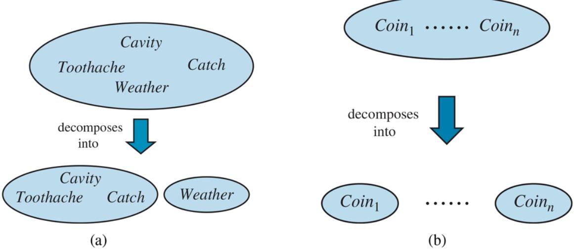
Two examples of factoring a large joint distribution into smaller distributions, using absolute independence. (a) Weather and dental problems are independent. (b) Coin flips are independent.

The property we used in Equation (12.10) is called independence (also marginal independence and absolute independence). In particular, the weather is independent of one’s dental problems. Independence between propositions and can be written as

(12.11)

\[P(a \mid b) = P(a) \quad \text{or} \quad P(b \mid a) = P(b) \quad \text{or} \quad P(a \land b) = P(a)P(b).\]

Independence

All these forms are equivalent (Exercise 12.INDI). Independence between variables and can be written as follows (again, these are all equivalent):

\[\mathbf{P}(X \mid Y) = \mathbf{P}(X) \quad \text{or} \quad \mathbf{P}(Y \mid X) = \mathbf{P}(Y) \quad \text{or} \quad \mathbf{P}(X, Y) = \mathbf{P}(X)\mathbf{P}(Y).\]

Independence assertions are usually based on knowledge of the domain. As the toothache– weather example illustrates, they can dramatically reduce the amount of information necessary to specify the full joint distribution. If the complete set of variables can be divided into independent subsets, then the full joint distribution can be factored into separate joint distributions on those subsets. For example, the full joint distribution on the outcome of

independent coin flips, , has entries, but it can be represented as the product of single-variable distributions . In a more practical vein, the independence of dentistry and meteorology is a good thing, because otherwise the practice of dentistry might require intimate knowledge of meteorology, and vice versa.

When they are available, then, independence assertions can help in reducing the size of the domain representation and the complexity of the inference problem. Unfortunately, clean separation of entire sets of variables by independence is quite rare. Whenever a connection, however indirect, exists between two variables, independence will fail to hold. Moreover, even independent subsets can be quite large—for example, dentistry might involve dozens of diseases and hundreds of symptoms, all of which are interrelated. To handle such problems, we need more subtle methods than the straightforward concept of independence.

12.5 Bayes’ Rule and Its Use

On page 390, we defined the product rule (Equation (12.4) ). It can actually be written in two forms:

\[P(a \wedge b) = P(a \mid b)P(b) \qquad \text{and} \qquad P(a \wedge b) = P(b \mid a)P(a).\]

Equating the two right-hand sides and dividing by , we get

(12.12)

\[P(b \mid a) = \frac{P(a \mid b)P(b)}{P(a)}.\]

This equation is known as Bayes’ rule (also Bayes’ law or Bayes’ theorem). This simple equation underlies most modern AI systems for probabilistic inference.

Bayes’ rule

The more general case of Bayes’ rule for multivalued variables can be written in the notation as follows:

\[\mathbf{P}(Y|X) = \frac{\mathbf{P}(X \mid Y)\mathbf{P}(Y)}{\mathbf{P}(X)}.\]

As before, this is to be taken as representing a set of equations, each dealing with specific values of the variables. We will also have occasion to use a more general version conditionalized on some background evidence :

(12.13)

\[\mathbf{P}(Y \mid X, \mathbf{e}) = \frac{\mathbf{P}(X \mid Y, \mathbf{e})\mathbf{P}(Y \mid \mathbf{e})}{\mathbf{P}(X \mid \mathbf{e})}.\]

12.5.1 Applying Bayes’ rule: The simple case

On the surface, Bayes’ rule does not seem very useful. It allows us to compute the single term in terms of three terms: , , and . That seems like two steps backwards; but Bayes’ rule is useful in practice because there are many cases where we do have good probability estimates for these three numbers and need to compute the fourth. Often, we perceive as evidence the effect of some unknown cause and we would like to determine that cause. In that case, Bayes’ rule becomes

\[P(cause \mid effect) = \frac{P(effect \mid cause)P(cause)}{P(effect)}.1\]

The conditional probability quantifies the relationship in the causal direction, whereas describes the diagnostic direction. In a task such as medical diagnosis, we often have conditional probabilities on causal relationships. The doctor knows ) and want to derive a diagnosis,

Causal

.

Diagnostic

For example, a doctor knows that the disease meningitis causes a patient to have a stiff neck, say, 70% of the time. The doctor also knows some unconditional facts: the prior probability that any patient has meningitis is and the prior probability that any patient has a stiff neck is 1%. Letting be the proposition that the patient has a stiff neck and be the proposition that the patient has meningitis, we have

(12.14)

\[\begin{aligned} P(s \mid m) &= 0.7\\ P(m) &= 1/50000\\ P(s) &= 0.01\\ P(m \mid s) &= \frac{P(s \mid m)P(m)}{P(s)} = \frac{0.7 \times 1/50000}{0.01} = 0.0014. \end{aligned}\]

That is, we expect only 0.14% of patients with a stiff neck to have meningitis. Notice that even though a stiff neck is quite strongly indicated by meningitis (with probability 0.7), the probability of meningitis in patients with stiff necks remains small. This is because the prior probability of stiff necks (from any cause) is much higher than the prior for meningitis.

Section 12.3 illustrated a process by which one can avoid assessing the prior probability of the evidence (here, ) by instead computing a posterior probability for each value of the query variable (here, and ) and then normalizing the results. The same process can be applied when using Bayes’ rule. We have

\[\mathbf{P}\left(M|s\right) = \alpha\left\langle P\left(s|m\right)P\left(m\right), P\left(s|\neg m\right)P\left(\neg m\right)\right\rangle.\]

Thus, to use this approach we need to estimate instead of . There is no free lunch—sometimes this is easier, sometimes it is harder. The general form of Bayes’ rule with normalization is

(12.15)

\[\mathbf{P}(Y \mid X) = \alpha \, \mathbf{P}(X \mid Y) \mathbf{P}(Y) \,,\]

where is the normalization constant needed to make the entries in sum to 1.

One obvious question to ask about Bayes’ rule is why one might have available the conditional probability in one direction, but not the other. In the meningitis domain, perhaps the doctor knows that a stiff neck implies meningitis in 1 out of 5000 cases; that is, the doctor has quantitative information in the diagnostic direction from symptoms to causes. Such a doctor has no need to use Bayes’ rule.

Unfortunately, diagnostic knowledge is often more fragile than causal knowledge. If there is a sudden epidemic of meningitis, the unconditional probability of meningitis, , will go up. The doctor who derived the diagnostic probability directly from statistical observation of patients before the epidemic will have no idea how to update the value, but the doctor who computes from the other three values will see that should go up proportionately with . Most important, the causal information is unaffected by the epidemic, because it simply reflects the way meningitis works. The use of this kind of direct causal or model-based knowledge provides the crucial robustness needed to make probabilistic systems feasible in the real world.

12.5.2 Using Bayes’ rule: Combining evidence

We have seen that Bayes’ rule can be useful for answering probabilistic queries conditioned on one piece of evidence—for example, the stiff neck. In particular, we have argued that probabilistic information is often available in the form . What happens when we have two or more pieces of evidence? For example, what can a dentist conclude if her nasty steel probe catches in the aching tooth of a patient? If we know the full joint distribution (Figure 12.3 ), we can read off the answer:

\(\mathbf{P}\left(Cavity\,\middle|\,\left|\,\left(toothache\wedge\!\!\right.0ch\right.\right)\right.\left.\left.\alpha\left(\ 0.108,0.016\right)\right.\left.\alpha\left(\ \left.\alpha\right.\left.\right.\right.\left.\alpha\left(\ \left.\alpha\right.\right.\right.\right.\left.\alpha\left(\ \left.\alpha\right.\right.\right.\right.\left.\alpha\left(\ \left.\alpha\right.\right.\right.\right.\left.\alpha\left(\ \left.\alpha\right.\right.\right.\right.\left.\alpha\left(\ \left.\alpha\right.\right.\right.\left.\alpha\left(\ \left.\alpha\right.\right.\right.\right.\left.\alpha\left(\ \left.\alpha\right.\right.\right.\right.\left.\alpha\left(\ \left.\alpha\right.\right.\right.\left.\alpha\left(\ \left.\alpha\right.\right.\right.\right.\left.\alpha\left(\ \left.\alpha\right.\right.\right.\left.\alpha\left(\ \left.\alpha\right.\right.\right.\right.\left.\alpha\left(\ \left.\alpha\right.\right.\right.\left.\alpha\left(\ \left.\alpha\right.\right.\right.\right.\left.\alpha\left(\ \left.\alpha\right.\right.\right.\left.\alpha\left(\ \left.\alpha\right.\right.\right.\right.\left.\alpha\left(\ \left.\alpha\right.\right.\right.\left.\alpha\left(\ \left.\alpha\right.\right.\right.\left.\alpha\left(\ \left.\alpha\right.\right.\right.\right.\left.\alpha\left(\ \left.\alpha\right.\right.\right.\left.\alpha\left(\ \left.\alpha\right.\right.\right.\left.\alpha\left(\ \left.\alpha\right.\right.\right.\left.\alpha\left(\ \left.\alpha\right.\right.\right.\right.\left.\alpha\left(\ \left.\alpha\right.\right.\right.\left.\alpha\left(\ \left.\alpha\right.\right.\right.\right.\left.\alpha\left(\ \left.\alpha\right.\right.\right.\right.\ldots\left}\right.\right.\alpha\left\)

We know, however, that such an approach does not scale up to larger numbers of variables. We can try using Bayes’ rule to reformulate the problem:

(12.16)

\[\begin{aligned} &\mathbf{P}\left(Cavity \,|\, tootherhae\wedge catch\right) \\ &= \alpha \mathbf{P}\left(toothache\wedge catch \,|\, Cavity\right) \mathbf{P}\left(Cavity\right). \end{aligned}\]

For this reformulation to work, we need to know the conditional probabilities of the conjunction for each value of . That might be feasible for just two evidence variables, but again it does not scale up. If there are possible evidence variables (X rays, diet, oral hygiene, etc.), then there are possible combinations of observed values for which we would need to know conditional probabilities. This is no better than using the full joint distribution.

To make progress, we need to find some additional assertions about the domain that will enable us to simplify the expressions. The notion of independence in Section 12.4 provides a clue, but needs refining. It would be nice if and were

independent, but they are not: if the probe catches in the tooth, then it is likely that the tooth has a cavity and that the cavity causes a toothache. These variables are independent, however, given the presence or the absence of a cavity. Each is directly caused by the cavity, but neither has a direct effect on the other: toothache depends on the state of the nerves in the tooth, whereas the probe’s accuracy depends primarily on the dentist’s skill, to which the toothache is irrelevant. Mathematically, this property is written as 7

7 We assume that the patient and dentist are distinct individuals.

(12.17)

This equation expresses the conditional independence of and given . We can plug it into Equation (12.16) to obtain the probability of a cavity:

(12.18)

\[\begin{aligned} &\mathbf{P}\left(Cavity\,\middle|\, toothache\wedge\, tach\right) \\ &= \alpha \mathbf{P}\left(toothache\mid Cavity\right)\,\mathbf{P}\left(catch\mid Cavity\right)\,\mathbf{P}\left(Cavity\right)\,.\end{aligned}\]

Conditional independence

Now the information requirements are the same as for inference, using each piece of evidence separately: the prior probability for the query variable and the conditional probability of each effect, given its cause.

The general definition of conditional independence of two variables and , given a third variable , is

\[\mathbf{P}(X, Y \mid Z) = \mathbf{P}(X \mid Z)\mathbf{P}(Y \mid Z).\]

In the dentist domain, for example, it seems reasonable to assert conditional independence of the variables and , given :

(12.19)

\[\mathbf{P}(Toolhache, Catch \mid Cavity) = \mathbf{P}(Toolhache \mid Cavity)\mathbf{P}(Catch \mid Cavity).\]

Notice that this assertion is somewhat stronger than Equation (12.17) , which asserts independence only for specific values of and . As with absolute independence in Equation (12.11) , the equivalent forms

\[\mathbf{P}(X \mid Y, Z) = \mathbf{P}(X \mid Z) \quad \text{and} \quad \mathbf{P}(Y \mid X, Z) = \mathbf{P}(Y \mid Z)\]

can also be used (see Exercise 12.PXYZ). Section 12.4 showed that absolute independence assertions allow a decomposition of the full joint distribution into much smaller pieces. It turns out that the same is true for conditional independence assertions. For example, given the assertion in Equation (12.19) , we can derive a decomposition as follows:

(The reader can easily check that this equation does in fact hold in Figure 12.3 .) In this way, the original large table is decomposed into three smaller tables. The original table has 7 independent numbers. (The table has entries, but they must sum to 1, so 7 are independent). The smaller tables contain a total of independent numbers. (For a conditional probability distribution such as there are two rows of two numbers, and each row sums to 1, so that’s two independent numbers; for a prior distribution such as there is only one independent number.) Going from 7 to 5 might not seem like a major triumph, but the gains can be much greater with larger number of symptoms.

In general, for symptoms that are all conditionally independent given , the size of the representation grows as instead of . That means that conditional independence assertions can allow probabilistic systems to scale up; moreover, they are much more commonly available than absolute independence assertions. Conceptually, separates and because it is a direct cause of both of them. The decomposition of large probabilistic domains into weakly connected subsets through conditional independence is one of the most important developments in the recent history of AI.

Separation

12.6 Naive Bayes Models

The dentistry example illustrates a commonly occurring pattern in which a single cause directly influences a number of effects, all of which are conditionally independent, given the cause. The full joint distribution can be written as

(12.20)

\[\mathbf{P}(Cause, Effect\_1, \dots, Effect\_n) = \mathbf{P}(Cause) \prod \mathbf{P}(Effect\_i \mid Cause).\]

Such a probability distribution is called a naive Bayes model—“naive” because it is often used (as a simplifying assumption) in cases where the “effect” variables are not strictly independent given the cause variable. (The naive Bayes model is sometimes called a Bayesian classifier, a somewhat careless usage that has prompted true Bayesians to call it the idiot Bayes model.) In practice, naive Bayes systems often work very well, even when the conditional independence assumption is not strictly true.

Naive Bayes

To use a naive Bayes model, we can apply Equation (12.20) to obtain the probability of the cause given some observed effects. Call the observed effects , while the remaining effect variables are unobserved. Then the standard method for inference from the joint distribution (Equation (12.9) ) can be applied:

\[\mathbf{P}(Cause\mid \mathbf{e}) = \alpha \sum\_{\mathbf{y}} \mathbf{P}(Cause, \mathbf{e}, \mathbf{y}).\]

From Equation (12.20) , we then obtain

(12.21)

\[\begin{aligned} \mathbf{P}(Cause \mid \mathbf{e}) &= \ \alpha \sum\_{\mathbf{y}} \mathbf{P} \left( Cause \right) \mathbf{P} \left( \mathbf{y} \mid Cause \right) \left( \prod\_{j} \mathbf{P} \left( e\_{j} \mid Cause \right) \right) \\ &= \ \alpha \mathbf{P} \left( Cause \right) \left( \prod\_{j} \mathbf{P} \left( e\_{j} \mid Cause \right) \right) \sum\_{\mathbf{y}} \mathbf{P} \left( \mathbf{y} \mid Cause \right) \\ &= \ \alpha \mathbf{P} \left( Cause \right) \prod\_{j} \mathbf{P} \left( e\_{j} \mid Cause \right) \end{aligned}\]

where the last line follows because the summation over is 1. Reinterpreting this equation in words: for each possible cause, multiply the prior probability of the cause by the product of the conditional probabilities of the observed effects given the cause; then normalize the result. The run time of this calculation is linear in the number of observed effects and does not depend on the number of unobserved effects (which may be very large in domains such as medicine). We will see in the next chapter that this is a common phenomenon in probabilistic inference: evidence variables whose values are unobserved usually “disappear” from the computation altogether.

12.6.1 Text classification with naive Bayes

Let’s see how a naive Bayes model can be used for the task of text classification: given a text, decide which of a predefined set of classes or categories it belongs to. Here the “cause” is the variable, and the “effect” variables are the presence or absence of certain key words, . Consider these two example sentences, taken from newspaper articles:

• 1. Stocks rallied on Monday, with major indexes gaining 1% as optimism persisted over the first quarter earnings season.
• 2. Heavy rain continued to pound much of the east coast on Monday, with flood warnings issued in New York City and other locations.

Text classification

The task is to classify each sentence into a —the major sections of the newspaper: , , , , or . The naive Bayes model consists of the prior probabilities and the conditional probabilities .

For each category , is estimated as the fraction of all previously seen documents that are of category . For example, if 9% of articles are about weather, we set . Similarly, is estimated as the fraction of documents of each category that contain word ; perhaps 37% of articles about business contain word 6, “stocks,” so is set to 0.37. 8

8 One needs to be careful not to assign probability zero to words that have not been seen previously in a given category of documents, since the zero would wipe out all the other evidence in Equation (12.21) . Just because you haven’t seen a word yet doesn’t mean you will never see it. Instead, reserve a small portion of the probability distribution to represent “previously unseen” words. See Chapter 20 for more on this issue in general, and Section 23.1.4 for the particular case of word models.

To categorize a new document, we check which key words appear in the document and then apply Equation (12.21) to obtain the posterior probability distribution over categories. If we have to predict just one category, we take the one with the highest posterior probability. Notice that, for this task, every effect variable is observed, since we can always tell whether a given word appears in the document.

The naive Bayes model assumes that words occur independently in documents, with frequencies determined by the document category. This independence assumption is clearly violated in practice. For example, the phrase “first quarter” occurs more frequently in business (or sports) articles than would be suggested by multiplying the probabilities of “first” and “quarter.” The violation of independence usually means that the final posterior probabilities will be much closer to 1 or 0 than they should be; in other words, the model is overconfident in its predictions. On the other hand, even with these errors, the ranking of the possible categories is often quite accurate.

Naive Bayes models are widely used for language determination, document retrieval, spam filtering, and other classification tasks. For tasks such as medical diagnosis, where the actual values of the posterior probabilities really matter—for example, in deciding whether to perform an appendectomy—one would usually prefer to use the more sophisticated models described in the next chapter.

12.7 The Wumpus World Revisited

We can combine the ideas in this chapter to solve probabilistic reasoning problems in the wumpus world. (See Chapter 7 for a complete description of the wumpus world.) Uncertainty arises in the wumpus world because the agent’s sensors give only partial information about the world. For example, Figure 12.5 shows a situation in which each of the three unvisited but reachable squares—[1,3], [2,2], and [3,1]—might contain a pit. Pure logical inference can conclude nothing about which square is most likely to be safe, so a logical agent might have to choose randomly. We will see that a probabilistic agent can do much better than the logical agent.

Figure 12.5

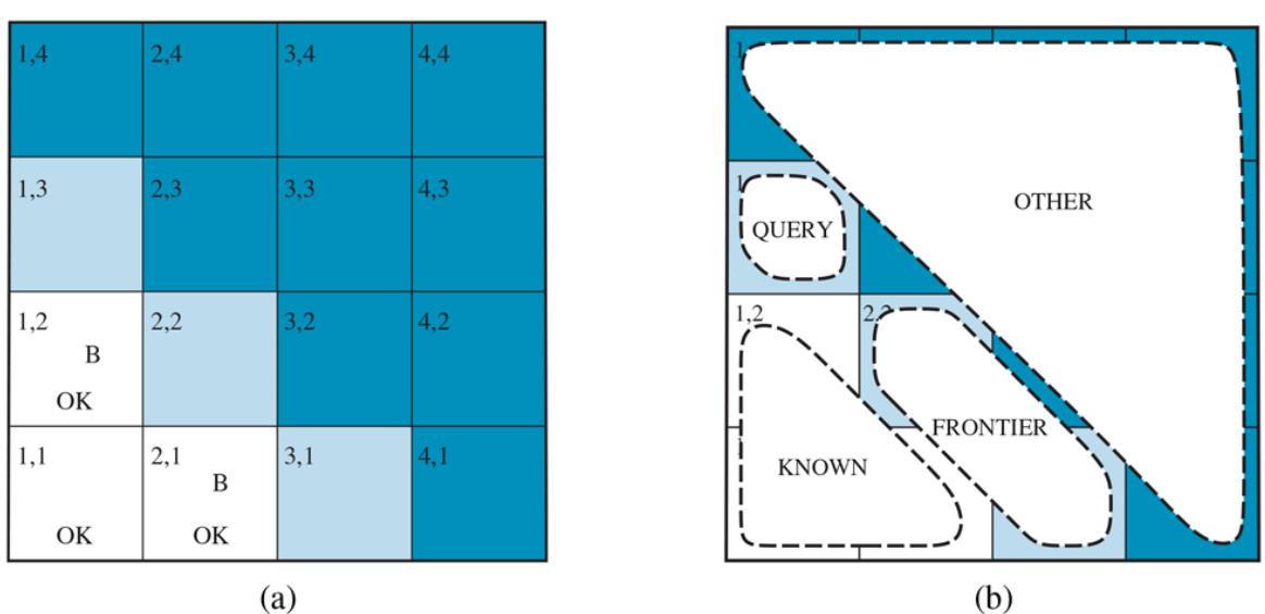
1. After finding a breeze in both [1,2] and [2,1], the agent is stuck—there is no safe place to explore. (b) Division of the squares into , , and , for a query about [1,3].

Our aim is to calculate the probability that each of the three squares contains a pit. (For this example we ignore the wumpus and the gold.) The relevant properties of the wumpus world are that (1) a pit causes breezes in all neighboring squares, and (2) each square other than [1,1] contains a pit with probability 0.2. The first step is to identify the set of random variables we need:

• As in the propositional logic case, we want one Boolean variable for each square, which is true iff square actually contains a pit.
• We also have Boolean variables that are true iff square is breezy; we include these variables only for the observed squares—in this case, [1,1], [1,2], and [2,1].

The next step is to specify the full joint distribution, . Applying the product rule, we have

\[\begin{aligned} \mathbf{P}(P\_{1,1}, \ldots, P\_{4,4}, B\_{1,1}, B\_{1,2}, B\_{2,1}) &= \\ \mathbf{P}\left(B\_{1,1}, B\_{1,2}, B\_{2,1} | P\_{1,1}, \ldots, P\_{4,4}\right) \mathbf{P}\left(P\_{1,1}, \ldots, P\_{4,4}\right) \end{aligned}\]

This decomposition makes it easy to see what the joint probability values should be. The first term is the conditional probability distribution of a breeze configuration, given a pit configuration; its values are 1 if all the breezy squares are adjacent to the pits and 0 otherwise. The second term is the prior probability of a pit configuration. Each square contains a pit with probability 0.2, independently of the other squares; hence,

(12.22)

\[\mathbf{P}(P\_{1,1}, \ldots, P\_{4,4}) = \prod\_{i,j=1,1}^{4,4} \mathbf{P}(P\_{i,j}).\]

For a particular configuration with exactly pits, the probability is .

In the situation in Figure 12.5(a) , the evidence consists of the observed breeze (or its absence) in each square that is visited, combined with the fact that each such square contains no pit. We abbreviate these facts as and . We are interested in answering queries such as : how likely is it that [1,3] contains a pit, given the observations so far?

To answer this query, we can follow the standard approach of Equation (12.9) , namely, summing over entries from the full joint distribution. Let be the set of variables for squares other than the known squares and the query square [1,3]. Then, by Equation (12.9) , we have

(12.23)

\[\mathbf{P}(P\_{1,3} \mid known, b) = \alpha \sum\_{unknown} \mathbf{P}(P\_{1,3}, known, b, unknown).\]

The full joint probabilities have already been specified, so we are done—that is, unless we care about computation. There are 12 unknown squares; hence the summation contains terms. In general, the summation grows exponentially with the number of squares.

Surely, one might ask, aren’t the other squares irrelevant? How could [4,4] affect whether [1,3] has a pit? Indeed, this intuition is roughly correct, but it needs to be made more precise. What we really mean is that if we knew the values of all the pit variables adjacent to the squares we care about, then pits (or their absence) in other, more distant squares could have no further effect on our belief.

Let be the pit variables (other than the query variable) that are adjacent to visited squares, in this case just [2,2] and [3,1]. Also, let be the pit variables for the other unknown squares; in this case, there are 10 other squares, as shown in Figure 12.5(b) . With these definitions, . The key insight given above can now be stated as follows: the observed breezes are conditionally independent of the other variables, given the known, frontier, and query variables. To use this insight, we manipulate the query formula into a form in which the breezes are conditioned on all the other variables, and then we apply conditional independence:

\[\begin{aligned} &\mathbf{P}(P\_{1,3}|known,b) \\ &= \alpha \sum\_{unknown} \mathbf{P}(P\_{1,3}, known, b, unknown) \qquad \text{(from Equation (12.23))} \\ &= \alpha \sum\_{unknown} \mathbf{P}(b|P\_{1,3}, known, unknown) \mathbf{P}(P\_{1,3}, known, unknown) \quad \text{(product rule)} \\ &= \alpha \sum\_{fromterior} \sum\_{other} \mathbf{P}(b|known, P\_{1,3}, frontier, other) \mathbf{P}(P\_{1,3}, known, fromterior, other) \\ &= \alpha \sum\_{fromterior} \sum\_{other} \mathbf{P}(b|known, P\_{1,3}, frontier) \mathbf{P}(P\_{1,3}, known, frontier, other), \end{aligned}\]

where the final step uses conditional independence: is independent of given , , and . Now, the first term in this expression does not depend on the variables, so we can move the summation inward:

\[\begin{aligned} &\mathbf{P}(P\_{1,3}|known, b) \\ &= \alpha \sum\_{froniter} \mathbf{P}(b|known, P\_{1,3}, frontier) \sum\_{other} \mathbf{P}(P\_{1,3}, known, frontier, other). \end{aligned}\]

By independence, as in Equation (12.22) , the term on the right can be factored, and then the terms can be reordered:

\[\begin{aligned} &\mathbf{P}(P\_{1,3}|known, b) \\ &= \alpha \sum\_{froniter} \mathbf{P}(b|known, P\_{1,3}, froniter) \sum\_{other} \mathbf{P}(P\_{1,3}) P(known) P(froniter) P(other) \\ &= \alpha P(known) \mathbf{P}(P\_{1,3}) \sum\_{froniter} \mathbf{P}(b|known, P\_{1,3}, froniter) P(froniter) \sum\_{other} P(other) \\ &= \alpha' \mathbf{P}(P\_{1,3}) \sum\_{froniter} \mathbf{P}(b|known, P\_{1,3}, froniter) P(froniter), \end{aligned}\]

where the last step folds into the normalizing constant and uses the fact that equals 1.

Now, there are just four terms in the summation over the frontier variables, and . The use of independence and conditional independence has completely eliminated the other squares from consideration.

Notice that the probabilities in are 1 when the breeze observations are consistent with the other variables and 0 otherwise. Thus, for each value of , we sum over the logical models for the frontier variables that are consistent with the known facts. (Compare with the enumeration over models in Figure 7.5 on page 215.) The models and their associated prior probabilities— —are shown in Figure 12.6 . We have

\[\mathbf{P}(P\_{1.3}|known, b) = \alpha' \left< 0.2 \langle 0.04 + 0.16 + 0.16 \right>, 0.8 \langle 0.04 + 0.16 \rangle \rangle \approx \langle 0.31, 0.69 \rangle\]

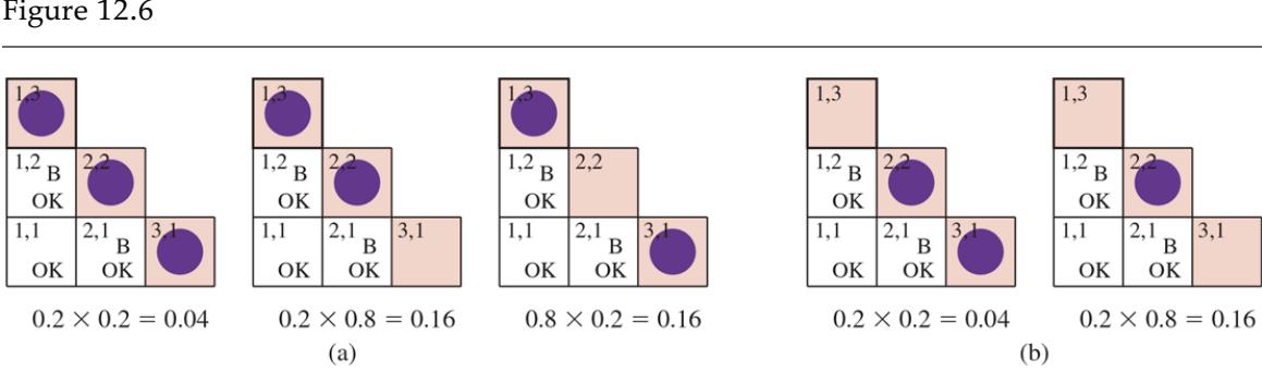
Consistent models for the frontier variables, and , showing for each model: (a) three models with showing two or three pits, and (b) two models with showing one or two pits.

That is, [1,3] (and [3,1] by symmetry) contains a pit with roughly 31% probability. A similar calculation, which the reader might wish to perform, shows that [2,2] contains a pit with roughly 86% probability. The wumpus agent should definitely avoid [2,2]! Note that our logical agent from Chapter 7 did not know that [2,2] was worse than the other squares. Logic can tell us that it is unknown whether there is a pit in [2, 2], but we need probability to tell us how likely it is.

What this section has shown is that even seemingly complicated problems can be formulated precisely in probability theory and solved with simple algorithms. To get efficient solutions, independence and conditional independence relationships can be used to simplify the summations required. These relationships often correspond to our natural understanding of how the problem should be decomposed. In the next chapter, we develop formal representations for such relationships as well as algorithms that operate on those representations to perform probabilistic inference efficiently.

Summary

This chapter has suggested probability theory as a suitable foundation for uncertain reasoning and provided a gentle introduction to its use.

• Uncertainty arises because of both laziness and ignorance. It is inescapable in complex, nondeterministic, or partially observable environments.
• Probabilities express the agent’s inability to reach a definite decision regarding the truth of a sentence. Probabilities summarize the agent’s beliefs relative to the evidence.
• Decision theory combines the agent’s beliefs and desires, defining the best action as the one that maximizes expected utility.
• Basic probability statements include prior or unconditional probabilities and posterior or conditional probabilities over simple and complex propositions.
• The axioms of probability constrain the probabilities of logically related propositions. An agent that violates the axioms must behave irrationally in some cases.
• The full joint probability distribution specifies the probability of each complete assignment of values to random variables. It is usually too large to create or use in its explicit form, but when it is available it can be used to answer queries simply by adding up entries for the possible worlds corresponding to the query propositions.
• Absolute independence between subsets of random variables allows the full joint distribution to be factored into smaller joint distributions, greatly reducing its complexity.
• Bayes’ rule allows unknown probabilities to be computed from known conditional probabilities, usually in the causal direction. Applying Bayes’ rule with many pieces of evidence runs into the same scaling problems as does the full joint distribution.
• Conditional independence brought about by direct causal relationships in the domain allows the full joint distribution to be factored into smaller, conditional distributions. The naive Bayes model assumes the conditional independence of all effect variables, given a single cause variable; its size grows linearly with the number of effects.
• A wumpus-world agent can calculate probabilities for unobserved aspects of the world, thereby improving on the decisions of a purely logical agent. Conditional independence makes these calculations tractable.

Bibliographical and Historical Notes

Probability theory was invented as a way of analyzing games of chance. In about 850 CE the Indian mathematician Mahaviracarya described how to arrange a set of bets that can’t lose (what we now call a Dutch book). In Europe, the first significant systematic analyses were produced by Girolamo Cardano around 1565, although publication was posthumous (1663). By that time, probability had been established as a mathematical discipline due to a series of results from a famous correspondence between Blaise Pascal and Pierre de Fermat in 1654. The first published textbook on probability was De Ratiociniis in Ludo Aleae (On Reasoning in a Game of Chance) by Huygens (1657). The “laziness and ignorance” view of uncertainty was described by John Arbuthnot in the preface of his translation of Huygens (Arbuthnot, 1692): “It is impossible for a Die, with such determin’d force and direction, not to fall on such determin’d side, only I don’t know the force and direction which makes it fall on such determin’d side, and therefore I call it Chance, which is nothing but the want of art.”

The connection between probability and reasoning dates back at least to the nineteenth century: in 1819, Pierre Laplace said, “Probability theory is nothing but common sense reduced to calculation.” In 1850, James Maxwell said, “The true logic for this world is the calculus of Probabilities, which takes account of the magnitude of the probability which is, or ought to be, in a reasonable man’s mind.”

There has been endless debate over the source and status of probability numbers. The frequentist position is that the numbers can come only from experiments: if we test 100 people and find that 10 of them have a cavity, then we can say that the probability of a cavity is approximately 0.1. In this view, the assertion “the probability of a cavity is 0.1” means that 0.1 is the fraction that would be observed in the limit of infinitely many samples. From any finite sample, we can estimate the true fraction and also calculate how accurate our estimate is likely to be.

Frequentist

The objectivist view is that probabilities are real aspects of the universe—propensities of objects to behave in certain ways—rather than being just descriptions of an observer’s degree of belief. For example, the fact that a fair coin comes up heads with probability 0.5 is a propensity of the coin itself. In this view, frequentist measurements are attempts to observe these propensities. Most physicists agree that quantum phenomena are objectively probabilistic, but uncertainty at the macroscopic scale—e.g., in coin tossing—usually arises from ignorance of initial conditions and does not seem consistent with the propensity view.

Objectivist

The subjectivist view describes probabilities as a way of characterizing an agent’s beliefs, rather than as having any external physical significance. The subjective Bayesian view allows any self-consistent ascription of prior probabilities to propositions, but then insists on proper Bayesian updating as evidence arrives.

Subjectivist

Even a strict frequentist position involves subjectivity because of the reference class problem: in trying to determine the outcome probability of a particular experiment, the frequentist has to place it in a reference class of “similar” experiments with known outcome frequencies. But what’s the right class? I. J. Good wrote, “every event in life is unique, and every real-life probability that we estimate in practice is that of an event that has never occurred before” (Good, 1983, p. 27).

Reference class

For example, given a particular patient, a frequentist who wants to estimate the probability of a cavity will consider a reference class of other patients who are similar in important ways —age, symptoms, diet—and see what proportion of them had a cavity. If the dentist considers everything that is known about the patient—hair color, weight to the nearest gram, mother’s maiden name—then the reference class becomes empty. This has been a vexing problem in the philosophy of science.

Pascal used probability in ways that required both the objective interpretation, as a property of the world based on symmetry or relative frequency, and the subjective interpretation, based on degree of belief—the former in his analyses of probabilities in games of chance, the latter in the famous “Pascal’s wager” argument about the possible existence of God. However, Pascal did not clearly realize the distinction between these two interpretations. The distinction was first drawn clearly by James Bernoulli (1654–1705).

Leibniz introduced the “classical” notion of probability as a proportion of enumerated, equally probable cases, which was also used by Bernoulli, although it was brought to prominence by Laplace (1816). This notion is ambiguous between the frequency interpretation and the subjective interpretation. The cases can be thought to be equally probable either because of a natural, physical symmetry between them, or simply because we do not have any knowledge that would lead us to consider one more probable than another. The use of this latter, subjective consideration to justify assigning equal probabilities is known as the principle of indifference. The principle is often attributed to Laplace (1816), but he never used the name explicitly; Keynes (1921) did. George Boole and John Venn both referred to it as the principle of insufficient reason.

Principle of indifference

Principle of insufficient reason

The debate between objectivists and subjectivists became sharper in the 20th century. Kolmogorov (1963), R. A. Fisher (1922), and Richard von Mises (1928) were advocates of the relative frequency interpretation. Karl Popper’s “propensity” interpretation (1959, first published in German in 1934) traces relative frequencies to an underlying physical symmetry. Frank Ramsey (1931), Bruno de Finetti (1937), R. T. Cox (1946), Leonard Savage (1954), Richard Jeffrey (1983), and E. T. Jaynes, (2003) interpreted probabilities as the degrees of belief of specific individuals. Their analyses of degree of belief were closely tied to utilities and to behavior—specifically, to the willingness to place bets.

Rudolf Carnap offered a different interpretation of probability—not as the degree of belief that an individual actually has, but as the degree of belief that an idealized reasoner should have in a particular proposition , given a particular body of evidence . Carnap attempted to make this notion of degree of confirmation mathematically precise, as a logical relation between and . Currently it is believed that there is no unique logic of this kind; rather, any such logic rests on a subjective prior probability distribution whose effect is diminished as more observations are collected.

The study of this relation was intended to constitute a mathematical discipline called inductive logic, analogous to ordinary deductive logic (Carnap, 1948, 1950). Carnap was not able to extend his inductive logic much beyond the propositional case, and Putnam (1963) showed by adversarial arguments that some difficulties were inherent. More recent work by Bacchus, Grove, Halpern, and Koller (1992) extends Carnap’s methods to first-order theories.

The first rigorously axiomatic framework for probability theory was proposed by Kolmogorov (1950, first published in German in 1933). Rényi (1970) later gave an axiomatic presentation that took conditional probability, rather than absolute probability, as primitive.

In addition to de Finetti’s arguments for the validity of the axioms, Cox (1946) showed that any system for uncertain reasoning that meets his set of assumptions is equivalent to probability theory. This gave renewed confidence to probability fans, but others were not convinced, objecting to the assumption that belief must be represented by a single number. Halpern (1999) describes the assumptions and shows some gaps in Cox’s original formulation. Horn (2003) shows how to patch up the difficulties. Jaynes (2003) has a similar argument that is easier to read.

The Rev. Thomas Bayes (1702–1761) introduced the rule for reasoning about conditional probabilities that was posthumously named after him (Bayes, 1763). Bayes only considered the case of uniform priors; it was Laplace who independently developed the general case. Bayesian probabilistic reasoning has been used in AI since the 1960s, especially in medical diagnosis. It was used not only to make a diagnosis from available evidence, but also to select further questions and tests by using the theory of information value (Section 16.6 ) when available evidence was inconclusive (Gorry, 1968; Gorry et al., 1973). One system outperformed human experts in the diagnosis of acute abdominal illnesses (de Dombal et al., 1974). Lucas et al. (2004) provide an overview.

These early Bayesian systems suffered from a number of problems. Because they lacked any theoretical model of the conditions they were diagnosing, they were vulnerable to unrepresentative data occurring in situations for which only a small sample was available (de Dombal et al., 1981). Even more fundamentally, because they lacked a concise formalism (such as the one to be described in Chapter 13 ) for representing and using conditional independence information, they depended on the acquisition, storage, and processing of enormous tables of probabilistic data. Because of these difficulties, probabilistic methods for coping with uncertainty fell out of favor in AI from the 1970s to the mid-1980s. Developments since the late 1980s are described in the next chapter.

The naive Bayes model for joint distributions has been studied extensively in the pattern recognition literature since the 1950s (Duda and Hart, 1973). It has also been used, often unwittingly, in information retrieval, beginning with the work of Maron (1961). The probabilistic foundations of this technique, described further in Exercise 12.BAYS, were elucidated by Robertson and Sparck Jones (1976). Domingos and Pazzani (1997) provide an explanation for the surprising success of naive Bayesian reasoning even in domains where the independence assumptions are clearly violated.

There are many good introductory textbooks on probability theory, including those by Bertsekas and Tsitsiklis (2008), Ross (2015), and Grinstead and Snell (1997). DeGroot and Schervish (2001) offer a combined introduction to probability and statistics from a Bayesian standpoint, and Walpole et al. (2016) offer an introduction for scientists and engineers. Jaynes (2003) gives a very persuasive exposition of the Bayesian approach. Billingsley (2012) and Venkatesh (2012) provide more mathematical treatments, including all the complications with continuous variables that we have left out. Hacking (1975) and Hald

(1990) cover the early history of the concept of probability, and Bernstein (1996) gives a popular account.

Chapter 13 Probabilistic Reasoning

In which we explain how to build efficient network models to reason under uncertainty according to the laws of probability theory, and how to distinguish between correlation and causality.

Chapter 12 introduced the basic elements of probability theory and noted the importance of independence and conditional independence relationships in simplifying probabilistic representations of the world. This chapter introduces a systematic way to represent such relationships explicitly in the form of Bayesian networks. We define the syntax and semantics of these networks and show how they can be used to capture uncertain knowledge in a natural and efficient way. We then show how probabilistic inference, although computationally intractable in the worst case, can be done efficiently in many practical situations. We also describe a variety of approximate inference algorithms that are often applicable when exact inference is infeasible. Chapter 15 extends the basic ideas of Bayesian networks to more expressive formal languages for defining probability models.

13.1 Representing Knowledge in an Uncertain Domain

In Chapter 12 , we saw that the full joint probability distribution can answer any question about the domain, but can become intractably large as the number of variables grows. Furthermore, specifying probabilities for possible worlds one by one is unnatural and tedious.

We also saw that independence and conditional independence relationships among variables can greatly reduce the number of probabilities that need to be specified in order to define the full joint distribution. This section introduces a data structure called a Bayesian network to represent the dependencies among variables. Bayesian networks can represent essentially any full joint probability distribution and in many cases can do so very concisely. 1

1 Bayesian networks, often often abbreviated to “Bayes net,” were called belief networks in the 1980s and 1990s. A causal network is a Bayes net with additional constraints on the meaning of the arrows (see Section 13.5 ). The term graphical model refers to a broader class that includes Bayesian networks.

Bayesian network

A Bayesian network is a directed graph in which each node is annotated with quantitative probability information. The full specification is as follows:

• 1. Each node corresponds to a random variable, which may be discrete or continuous.
• 2. Directed links or arrows connect pairs of nodes. If there is an arrow from node to node is said to be a parent of . The graph has no directed cycles and hence is a directed acyclic graph, or DAG.
• 3. Each node has associated probability information that quantifies the effect of the parents on the node using a finite number of parameters.

Parameter

The topology of the network—the set of nodes and links—specifies the conditional independence relationships that hold in the domain, in a way that will be made precise shortly. The intuitive meaning of an arrow is typically that has a direct influence on , which suggests that causes should be parents of effects. It is usually easy for a domain expert to decide what direct influences exist in the domain—much easier, in fact, than actually specifying the probabilities themselves. Once the topology of the Bayes net is laid out, we need only specify the local probability information for each variable, in the form of a conditional distribution given its parents. The full joint distribution for all the variables is defined by the topology and the local probability information.

Recall the simple world described in Chapter 12 , consisting of the variables , , , and . We argued that is independent of the other variables; furthermore, we argued that and are conditionally independent, given . These relationships are represented by the Bayes net structure shown in Figure 13.1 . Formally, the conditional independence of and , given , is indicated by the absence of a link between and . Intuitively, the network represents the fact that is a direct cause of and , whereas no direct causal relationship exists between and .

Figure 13.1

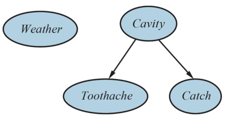
A simple Bayesian network in which is independent of the other three variables and and are conditionally independent, given .

Now consider the following example, which is just a little more complex. You have a new burglar alarm installed at home. It is fairly reliable at detecting a burglary, but is occasionally set off by minor earthquakes. (This example is due to Judea Pearl, a resident of earthquake-prone Los Angeles.) You also have two neighbors, John and Mary, who have promised to call you at work when they hear the alarm. John nearly always calls when he hears the alarm, but sometimes confuses the telephone ringing with the alarm and calls then, too. Mary, on the other hand, likes rather loud music and often misses the alarm altogether. Given the evidence of who has or has not called, we would like to estimate the probability of a burglary.

A Bayes net for this domain appears in Figure 13.2 . The network structure shows that burglary and earthquakes directly affect the probability of the alarm’s going off, but whether John and Mary call depends only on the alarm. The network thus represents our assumptions that they do not perceive burglaries directly, they do not notice minor earthquakes, and they do not confer before calling.

Figure 13.2

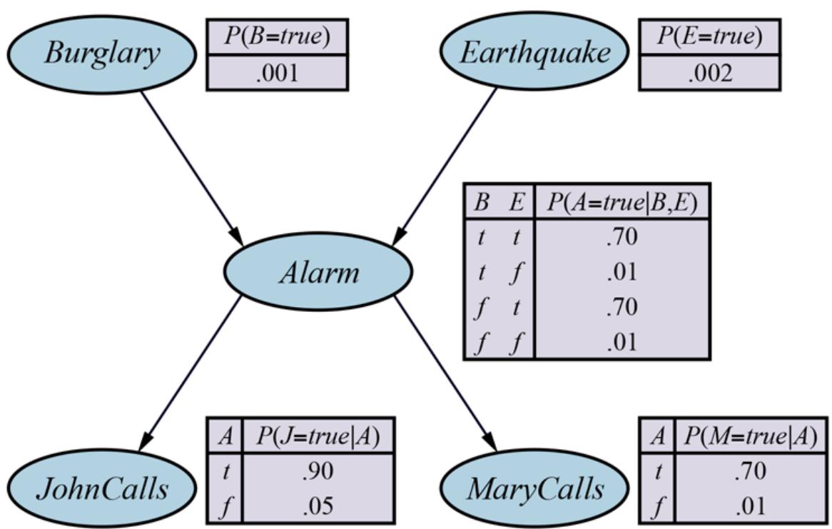
A typical Bayesian network, showing both the topology and the conditional probability tables (CPTs). In the CPTs, the letters , , , , and stand for Burglar, Earthquake, Alarm, , and , respectively.

The local probability information attached to each node in Figure 13.2 takes the form of a conditional probability table (CPT). (CPTs can be used only for discrete variables; other representations, including those suitable for continuous variables, are described in Section 13.2 .) Each row in a CPT contains the conditional probability of each node value for a conditioning case. A conditioning case is just a possible combination of values for the parent nodes—a miniature possible world, if you like. Each row must sum to 1, because the entries represent an exhaustive set of cases for the variable. For Boolean variables, once you know that the probability of a true value is , the probability of false must be , so we often omit the second number, as in Figure 13.2 . In general, a table for a Boolean variable with Boolean parents contains independently specifiable probabilities. A node with no parents has only one row, representing the prior probabilities of each possible value of the variable.

Conditional probability table (CPT)

Conditioning case

Notice that the network does not have nodes corresponding to Mary’s currently listening to loud music or to the telephone ringing and confusing John. These factors are summarized in the uncertainty associated with the links from Alarm to and . This shows both laziness and ignorance in operation, as explained on page 386: it would be a lot of work to find out why those factors would be more or less likely in any particular case, and we have no reasonable way to obtain the relevant information anyway.

The probabilities actually summarize a potentially infinite set of circumstances in which the alarm might fail to go off (high humidity, power failure, dead battery, cut wires, a dead mouse stuck inside the bell, etc.) or John or Mary might fail to call and report it (out to lunch, on vacation, temporarily deaf, passing helicopter, etc.). In this way, a small agent can cope with a very large world, at least approximately.

13.2 The Semantics of Bayesian Networks

The syntax of a Bayes net consists of a directed acyclic graph with some local probability information attached to each node. The semantics defines how the syntax corresponds to a joint distribution over the variables of the network.

Assume that the Bayes net contains variables, . A generic entry in the joint distribution is then , or for short. The semantics of Bayes nets defines each entry in the joint distribution as follows:

(13.1)

\[P(x\_1, \ldots, x\_n) = \prod\_{i=1}^n \theta(x\_i |parents(X\_i)),\]

where denotes the values of that appear in . Thus, each entry in the joint distribution is represented by the product of the appropriate elements of the local conditional distributions in the Bayes net.

To illustrate this, we can calculate the probability that the alarm has sounded, but neither a burglary nor an earthquake has occurred, and both John and Mary call. We simply multiply the relevant entries from the local conditional distributions (abbreviating the variable names):

\[\begin{aligned} P(j,m,a,\neg b,\neg e) &= P(j|a)P(m|a)P(a|\neg b \land \neg e)P(\neg b)P(\neg e) \\ &= 0.90 \times 0.70 \times 0.01 \times 0.999 \times 0.998 = 0.00628. \end{aligned}\]

Section 12.3 explained that the full joint distribution can be used to answer any query about the domain. If a Bayes net is a representation of the joint distribution, then it too can be used to answer any query, by summing all the relevant joint probability values, each calculated by multiplying probabilities from the local conditional distributions. Section 13.3 explains this in more detail, but also describes methods that are much more efficient.

So far, we have glossed over one important point: what is the meaning of the numbers that go into the local conditional distributions ? It turns out that from Equation (13.1) we can prove that the parameters are exactly the conditional probabilities implied by the joint distribution. Remember that the conditional probabilities can be computed from the joint distribution as follows:

\[\begin{aligned} P(x\_i |parents(X\_i)) &\equiv \frac{P(x\_i, parents(X\_i))}{P(parents(X\_i))}\\ &= \frac{\sum\_{\mathbf{y}} P(x\_i, parents(X\_i), \mathbf{y})}{\sum x\_i', \mathbf{y}P(x\_i', parents(X\_i), \mathbf{y})} \end{aligned}\]

where represents the values of all variables other than and its parents. From this last line one can prove that (Exercise 13.CPTE). Hence, we can rewrite Equation (13.1) as

(13.2)

\[P(x\_1, \ldots, x\_n) = \prod\_{i=1}^n P(x\_i |parent(X\_i)).\]

This means that when one estimates values for the local conditional distributions, they need to be the actual conditional probabilities for the variable given its parents. So, for example, when we specify , it should be the case that about 90% of the time when the alarm sounds, John calls. The fact that each parameter of the network has a precise meaning in terms of only a small set of variables is crucially important for robustness and ease of specification of the models.

A method for constructing Bayesian networks

Equation (13.2) defines what a given Bayes net means. The next step is to explain how to construct a Bayesian network in such a way that the resulting joint distribution is a good representation of a given domain. We will now show that Equation (13.2) implies certain conditional independence relationships that can be used to guide the knowledge engineer in constructing the topology of the network. First, we rewrite the entries in the joint distribution in terms of conditional probability, using the product rule (see page 390):

\[P(x\_1, \ldots, x\_n) = P(x\_n | x\_{n-1}, \ldots, x\_1) P(x\_{n-1}, \ldots, x\_1).\]

Then we repeat the process, reducing each joint probability to a conditional probability and a joint probability on a smaller set of variables. We end up with one big product:

\[P(x\_1, \ldots, x\_n) \quad = P(x\_n | x\_{n-1}, \ldots, x\_1) P(x\_{n-1} | x\_{n-2}, \ldots, x\_1) \quad \cdots P(x\_2 | x\_1) P(x\_1)\]

\[= \prod\_{i=1}^n P(x\_i | x\_{i-1}, \ldots, x\_1).\]

This identity is called the chain rule. It holds for any set of random variables. Comparing it with Equation (13.2) , we see that the specification of the joint distribution is equivalent to the general assertion that, for every variable in the network,

(13.3)

\[\mathbf{P}(X\_i|X\_{i-1},\ldots,X\_1) = \mathbf{P}(X\_i|Pareents(X\_i))\,,\]

Chain rule

provided that . This last condition is satisfied by numbering the nodes in topological order—that is, in any order consistent with the directed graph structure. For example, the nodes in Figure 13.2 could be ordered ; ; and so on.

Topological ordering

What Equation (13.3) says is that the Bayesian network is a correct representation of the domain only if each node is conditionally independent of its other predecessors in the node ordering, given its parents. We can satisfy this condition with this methodology:

• 1. NODES: First determine the set of variables that are required to model the domain. Now order them, . Any order will work, but the resulting network will be more compact if the variables are ordered such that causes precede effects.
• 2. LINKS: For to do:
  • Choose a minimal set of parents for from , such that Equation (13.3) is satisfied.
• For each parent insert a link from the parent to .
• CPTs: Write down the conditional probability table, .

Intuitively, the parents of node should contain all those nodes in that directly influence . For example, suppose we have completed the network in Figure 13.2 except for the choice of parents for . is certainly influenced by whether there is a Burglar or an Earthquake, but not directly influenced. Intuitively, our knowledge of the domain tells us that these events influence Mary’s calling behavior only through their effect on the alarm. Also, given the state of the alarm, whether John calls has no influence on Mary’s calling. Formally speaking, we believe that the following conditional independence statement holds:

Thus, Alarm will be the only parent node for .

Because each node is connected only to earlier nodes, this construction method guarantees that the network is acyclic. Another important property of Bayes nets is that they contain no redundant probability values. If there is no redundancy, then there is no chance for inconsistency: it is impossible for the knowledge engineer or domain expert to create a Bayesian network that violates the axioms of probability.

Compactness and node ordering

As well as being a complete and nonredundant representation of the domain, a Bayes net can often be far more compact than the full joint distribution. This property is what makes it feasible to handle domains with many variables. The compactness of Bayesian networks is an example of a general property of locally structured (also called sparse) systems. In a locally structured system, each subcomponent interacts directly with only a bounded number of other components, regardless of the total number of components. Local structure is usually associated with linear rather than exponential growth in complexity.

Locally structured

Sparse

In the case of Bayes nets, it is reasonable to suppose that in most domains each random variable is directly influenced by at most others, for some constant . If we assume Boolean variables for simplicity, then the amount of information needed to specify each conditional probability table will be at most numbers, and the complete network can be specified by numbers. In contrast, the joint distribution contains numbers. To make this concrete, suppose we have nodes, each with five parents ( ). Then the Bayesian network requires 960 numbers, but the full joint distribution requires over a billion.

Specifying the conditional probability tables for a fully connected network, in which each variable has all of its predecessors as parents, requires the same amount of information as specifying the joint distribution in tabular form. For this reason, we often leave out links even though a slight dependency exists, because the slight gain in accuracy is not worth the the additional complexity in the network. For example, one might object to our burglary network on the grounds that if there is a large earthquake, then John and Mary would not call even if they heard the alarm, because they assume that the earthquake is the cause. Whether to add the link from Earthquake to and (and thus enlarge the tables) depends on the importance of getting more accurate probabilities compared with the cost of specifying the extra information.

Even in a locally structured domain, we will get a compact Bayes net only if we choose the node ordering well. What happens if we happen to choose the wrong order? Consider the burglary example again. Suppose we decide to add the nodes in the order , , Alarm, Burglar, Earthquake. We then get the somewhat more complicated network shown in Figure 13.3(a) . The process goes as follows:

• Adding : No parents.
• Adding : If Mary calls, that probably means the alarm has gone off, which makes it more likely that John calls. Therefore, needs as a parent.
• Adding Alarm: Clearly, if both call, it is more likely that the alarm has gone off than if just one or neither calls, so we need both and as parents.

Adding Burglar: If we know the alarm state, then the call from John or Mary might give us information about our phone ringing or Mary’s music, but not about burglary:

Hence we need just Alarm as parent.

Adding Earthquake: If the alarm is on, it is more likely that there has been an earthquake. (The alarm is an earthquake detector of sorts.) But if we know that there has been a burglary, then that explains the alarm, and the probability of an earthquake would be only slightly above normal. Hence, we need both Alarm and Burglar as parents.

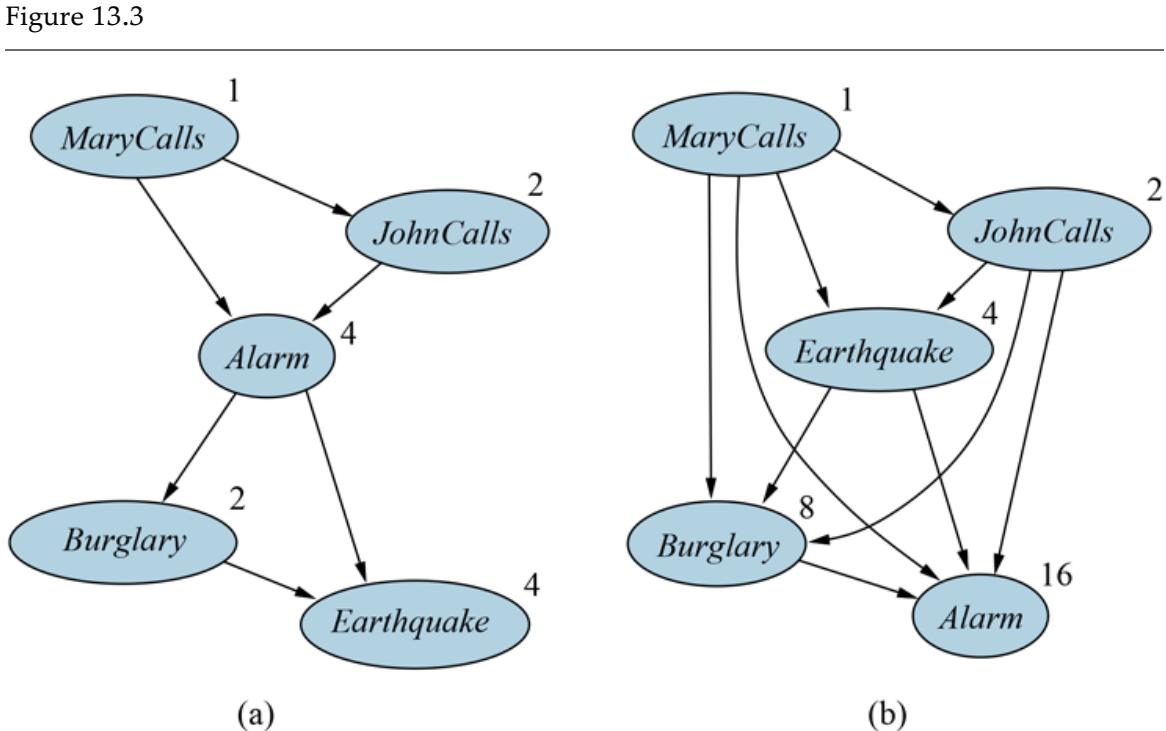
Network structure and number of parameters depends on order of introduction. (a) The structure obtained with ordering . (b) The structure obtained with . Each node is annotated with the number of parameters required; 13 in all for (a) and 31 for (b). In Figure 13.2 , only 10 parameters were required.

The resulting network has two more links than the original network in Figure 13.2 and requires 13 conditional probabilities rather than 10. What’s worse, some of the links represent tenuous relationships that require difficult and unnatural probability judgments, such as assessing the probability of Earthquake, given Burglar and Alarm. This phenomenon is quite general and is related to the distinction between causal and diagnostic models introduced in Section 12.5.1 (see also Exercise 13.WUMD). If we stick to a causal model, we end up having to specify fewer numbers, and the numbers will often be easier to come up with. For example, in the domain of medicine, it has been shown by Tversky and Kahneman (1982) that expert physicians prefer to give probability judgments for causal rules rather than for diagnostic ones. Section 13.5 explores the idea of causal models in more depth.

Figure 13.3(b) shows a very bad node ordering: , , Earthquake, Burglar, Alarm. This network requires 31 distinct probabilities to be specified—exactly the same number as the full joint distribution. It is important to realize, however, that any of the three networks can represent exactly the same joint distribution. The two versions in Figure 13.3 simply fail to represent all the conditional independence relationships and hence end up specifying a lot of unnecessary numbers instead.

13.2.1 Conditional independence relations in Bayesian networks

From the semantics of Bayes nets as defined in Equation (13.2) , we can derive a number of conditional independence properties. We have already seen the property that a variable is conditionally independent of its other predecessors, given its parents. It is also possible to prove the more general “non-descendants” property that:

Each variable is conditionally independent of its non-descendants, given its parents.

Descendant

For example, in Figure 13.2 , the variable is independent of Burglar, Earthquake, and given the value of Alarm. The definition is illustrated in Figure 13.4(a) .

Figure 13.4

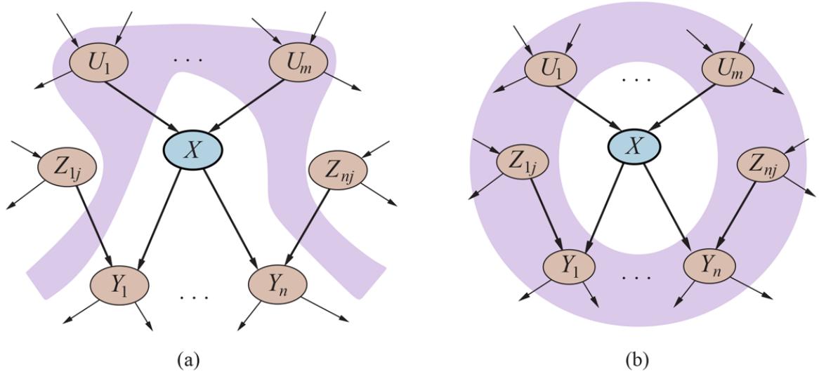
1. A node is conditionally independent of its non-descendants (e.g., the s) given its parents (the s shown in the gray area). (b) A node is conditionally independent of all other nodes in the network given its Markov blanket (the gray area).

It turns out that the non-descendants property combined with interpretation of the network parameters as conditional probabilities suffices to reconstruct the full joint distribution given in Equation (13.2) . In other words, one can view the semantics of Bayes nets in a different way: instead of defining the full joint distribution as the product of conditional distributions, the network defines a set of conditional independence properties. The full joint distribution can be derived from those properties.

Another important independence property is implied by the non-descendants property:

a variable is conditionally independent of all other nodes in the network, given its parents, children, and children’s parents—that is, given its Markov blanket.

Markov blanket

(Exercise 13.MARB asks you to prove this.) For example, the variable Burglary is independent of and , given Alarm and Earthquake. This property is illustrated in Figure 13.4(b) . The Markov blanket property makes possible inference algorithms that use completely local and distributed stochastic sampling processes, as explained in Section 13.4.2 .

The most general conditional independence question one might ask in a Bayes net is whether a set of nodes is conditionally independent of another set , given a third set . This can be determined efficiently by examining the Bayes net to see whether d-separates and . The process works as follows:

D-separation

1. Consider just the ancestral subgraph consisting of , , , and their ancestors.

Ancestral subgraph

2. Add links between any unlinked pair of nodes that share a common child; now we have the so-called moral graph.

Moral graph

• 3. Replace all directed links by undirected links.
• 4. If blocks all paths between and in the resulting graph, then d-separates and . In that case, is conditionally independent of , given . Otherwise, the original Bayes net does not require conditional independence.

In brief, then, d-separation means separation in the undirected, moralized, ancestral subgraph. Applying the definition to the burglary network in Figure 13.2 , we can deduce that Burglar and Earthquake are independent given the empty set (i.e., they are absolutely independent); that they are not necessarily conditionally independent given Alarm; and that and are conditionally independent given Alarm. Notice also that the Markov blanket property follows directly from the d-separation property, since a variable’s Markov blanket d-separates it from all other variables.

13.2.2 Efficient Representation of Conditional Distributions

Even if the maximum number of parents is smallish, filling in the CPT for a node requires up to numbers and perhaps a great deal of experience with all the possible conditioning cases. In fact, this is a worst-case scenario in which the relationship between the parents and the child is completely arbitrary. Usually, such relationships are describable by a canonical distribution that fits some standard pattern. In such cases, the complete table can be specified just by naming the pattern and perhaps supplying a few parameters.

Canonical distribution

The simplest example is provided by deterministic nodes. A deterministic node has its value specified exactly by the values of its parents, with no uncertainty. The relationship can be a logical one: for example, the relationship between the parent nodes , , and the child node is simply that the child is the disjunction of the parents. The relationship can also be numerical: for example, the for a car is the minimum of the prices at each dealer in the area; and the in a reservoir at year’s end is the sum of the original amount, plus the inflows (rivers, runoff, precipitation) and minus the outflows (releases, evaporation, seepage).

Deterministic nodes

Many Bayes net systems allow the user to specify deterministic functions using a generalpurpose programming language; this makes it possible to include complex elements such as global climate models or power-grid simulators within a probabilistic model.

Another important pattern that occurs often in practice is context-specific independence or CSI. A conditional distribution exhibits CSI if a variable is conditionally independent of some of its parents given certain values of others. For example, let’s suppose that the to your car occurring during a given period of time depends on the of your car and whether or not an occurred in that period. Clearly, if is false, then the , if any, doesn’t depend on the of your car. (There might be vandalism damage to the car’s paintwork or windows, but we’ll assume all cars are equally subject to such damage.) We say that is context-specifically independent of given . Bayes net systems often implement CSI using an ifthen-else syntax for specifying conditional distributions; for example, one might write

Context-specific independence

where and represent arbitrary distributions. As with determinism, the presence of CSI in a network may facilitate efficient inference. All of the exact inference algorithms mentioned in Section 13.3 can be modified to take advantage of CSI to speed up computation.

Uncertain relationships can often be characterized by so-called noisy logical relationships. The standard example is the noisy-OR relation, which is a generalization of the logical OR. In propositional logic, we might say that is true if and only if , , or are true. The noisy-OR model allows for uncertainty about the ability of each parent to cause the child to be true—the causal relationship between parent and child may be inhibited, and so a patient could have a cold, but not exhibit a fever.

Noisy-OR

The model makes two assumptions. First, it assumes that all the possible causes are listed. (If some are missing, we can always add a so-called leak node that covers “miscellaneous causes.”) Second, it assumes that inhibition of each parent is independent of inhibition of any other parents: for example, whatever inhibits from causing a fever is independent of whatever inhibits from causing a fever. Given these assumptions, is false if and only if all its true parents are inhibited, and the probability of this is the product of the inhibition probabilities for each parent. Let us suppose these individual inhibition probabilities are as follows:

\[\begin{aligned} q\_{\text{cold}} &= P(\neg fewer|cold, \neg filu, \neg malaria) = 0.6, \\ q\_{\text{flu}} &= P(\neg fewer|\negcold, flu, \neg malaria) = 0.2, \\ q\_{\text{malaria}} &= P(\neg fewer|\negcold, \neg filu, malaria) = 0.1. \end{aligned}\]

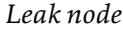
Then, from this information and the noisy-OR assumptions, the entire CPT can be built. The general rule is that

\[P(x\_i |parents(X\_i)) = 1 - \prod\_{\{j: X\_j = true\}} q\_j\,,\]

where the product is taken over the parents that are set to true for that row of the CPT. Figure 13.5 illustrates this calculation.

Figure 13.5

Cold				Flu Malaria P(fever . ) P(-fever . )
f	f	f	0.0	1.0
f	f	t	0.9	0.1
f	t	f	0.8	0.2
f	t	t	0.98	0.02 = 0.2 × 0.1
t	f	f	0.4	0.6
t	f	t	0.94	0.06 = 0.6×0.1
t	t	f	0.88	0.12 = 0.6×0.2
t	t	t	0.988	0.012 = 0.6×0.2×0.1

In general, noisy logical relationships in which a variable depends on parents can be described using parameters instead of for the full conditional probability table. This makes assessment and learning much easier. For example, the CPCS network (Pradhan et al., 1994) uses noisy-OR and noisy-MAX distributions to model relationships among diseases and symptoms in internal medicine. With 448 nodes and 906 links, it requires only 8,254 parameters instead of 133,931,430 for a network with full CPTs.

13.2.3 Bayesian nets with continuous variables

Many real-world problems involve continuous quantities, such as height, mass, temperature, and money. By definition, continuous variables have an infinite number of possible values, so it is impossible to specify conditional probabilities explicitly for each value. One way to handle continuous variables is with discretization—that is, dividing up the possible values into a fixed set of intervals. For example, temperatures could be divided into three categories: ( ), ( ), and ( ). In choosing the number of categories, there is a tradeoff between loss of accuracy and large CPTs which can lead to slow run times.

Discretization

Another approach is to define a continuous variable using one of the standard families of probability density functions (see Appendix A ). For example, a Gaussian (or normal) distribution is specified by just two parameters, the mean and the variance . Yet another solution—sometimes called a nonparametric representation—is to define the conditional distribution implicitly with a collection of instances, each containing specific values of the parent and child variables. We explore this approach further in Chapter 19 .

A network with both discrete and continuous variables is called a hybrid Bayesian network. To specify a hybrid network, we have to specify two new kinds of distributions: the conditional distribution for a continuous variable given discrete or continuous parents; and the conditional distribution for a discrete variable given continuous parents. Consider the simple example in Figure 13.6 , in which a customer buys some fruit depending on its cost, which depends in turn on the size of the harvest and whether the government’s subsidy scheme is operating. The variable is continuous and has continuous and discrete parents; the variable is discrete and has a continuous parent.

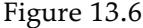
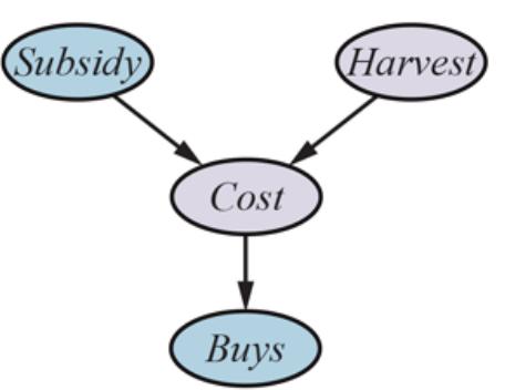
A simple network with discrete variables ( and ) and continuous variables ( and ).

Hybrid Bayesian network

For the variable, we need to specify . The discrete parent is handled by enumeration—that is, by specifying both and . To handle , we specify how the distribution over the cost depends on the continuous value of . In other words, we specify the parameters of the cost distribution as a function of . The most common choice is the linear– Gaussian conditional distribution, in which the child has a Gaussian distribution whose mean varies linearly with the value of the parent and whose standard deviation is fixed. We need two distributions, one for and one for , with different parameters:

\[P(c|h, subsidy) = N(c; a\_t h + b\_t, \sigma\_t^2) = \frac{1}{\sigma\_t \sqrt{2\pi}} e^{-\frac{1}{2} \left(\frac{c - (a\_t h + b\_t)}{\sigma\_t}\right)^2}\]

\[P(c|h, \neg subsidy) = N(c; a\_f h + b\_f, \sigma\_f^2) = \frac{1}{\sigma\_f \sqrt{2\pi}} e^{-\frac{1}{2} \left(\frac{c - (a\_f h + b\_f)}{\sigma\_f}\right)^2}.\]

Linear–Gaussian

For this example, then, the conditional distribution for is specified by naming the linear–Gaussian distribution and providing the parameters , , , , , and . Figures 13.7(a) and (b) show these two relationships. Notice that in each case the slope of versus is negative, because cost decreases as the harvest size increases. (Of course, the assumption of linearity implies that the cost becomes negative at some point; the linear model is reasonable only if the harvest size is limited to a narrow range.) Figure 13.7(c) shows the distribution , averaging over the two possible values of and assuming that each has prior probability 0.5. This shows that even with very simple models, quite interesting distributions can be represented.

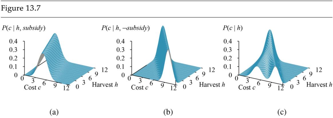
The graphs in (a) and (b) show the probability distribution over as a function of size, with true and false, respectively. Graph (c) shows the distribution , obtained by summing over the two subsidy cases.

The linear–Gaussian conditional distribution has some special properties. A network containing only continuous variables with linear–Gaussian distributions has a joint distribution that is a multivariate Gaussian distribution (see Appendix A ) over all the variables (Exercise 13.LGEX). Furthermore, the posterior distribution given any evidence also has this property. When discrete variables are added as parents (not as children) of continuous variables, the network defines a conditional Gaussian, or CG, distribution: given any assignment to the discrete variables, the distribution over the continuous variables is a multivariate Gaussian. 2

2 It follows that inference in linear–Gaussian networks takes only time in the worst case, regardless of the network topology. In Section 13.3 , we see that inference for networks of discrete variables is NPhard.

Conditional Gaussian

Now we turn to the distributions for discrete variables with continuous parents. Consider, for example, the node in Figure 13.6 . It seems reasonable to assume that the customer will buy if the cost is low and will not buy if it is high and that the probability of buying varies smoothly in some intermediate region. In other words, the conditional distribution is like a “soft” threshold function. One way to make soft thresholds is to use the integral of the standard normal distribution:

\[\Phi(x) = \int\_{-\infty}^{x} N(s; 0, 1) ds.\]

is an increasing function of , whereas the probability of buying decreases with cost, so here we flip the function around:

\[P(buss|Cost = c) = 1 - \Phi((c - \mu)/\sigma),\]

which means that the cost threshold occurs around , the width of the threshold region is proportional to , and the probability of buying decreases as cost increases. This probit model (pronounced “pro-bit” and short for “probability unit”) is illustrated in Figure

13.8(a) . The form can be justified by proposing that the underlying decision process has a hard threshold, but that the precise location of the threshold is subject to random Gaussian noise.

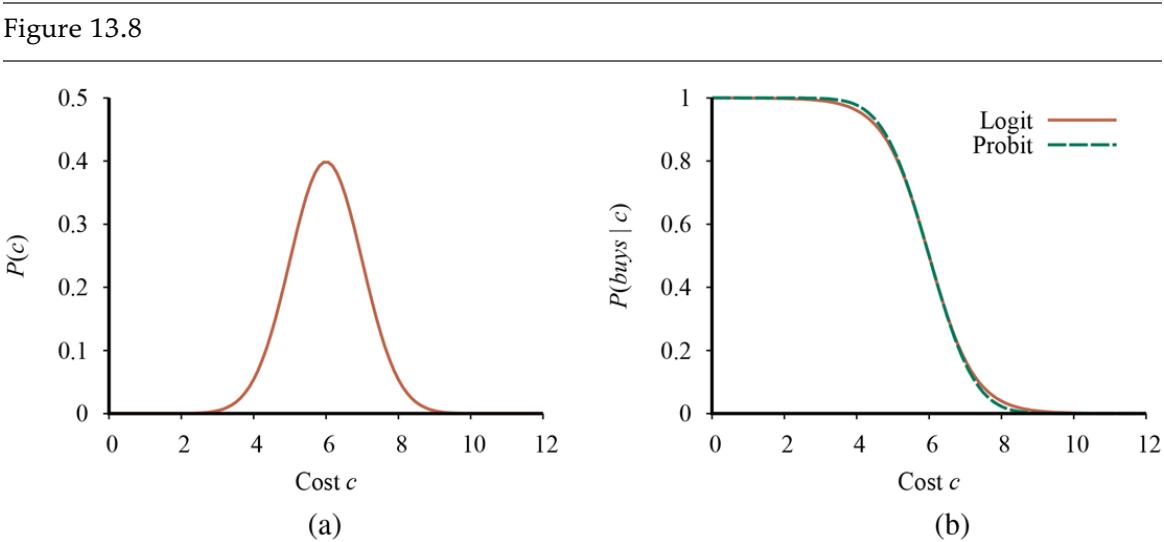
1. A normal (Gaussian) distribution for the cost threshold, centered on with standard deviation . (b) Expit and probit models for the probability of given , for the parameters and .

Probit

An alternative to the probit model is the expit or inverse logit model. It uses the logistic function to produce a soft threshold—it maps any to a value between 0 and 1. Again, for our example, we flip it around to make a decreasing function; we also scale the exponent by to match the probit’s slope at the mean:

\[P(buss|Cost = c) = 1 - \frac{1}{1 + exp(-\frac{4}{\sqrt{2\pi}} \cdot \frac{c - \mu}{\sigma})}\]

Expit

Inverse logit

Logistic function

This is illustrated in Figure 13.8(b) . The two distributions look similar, but the logit actually has much longer “tails.” The probit is often a better fit to real situations, but the logistic function is sometimes easier to deal with mathematically. It is used widely in machine learning. Both models can be generalized to handle multiple continuous parents by taking a linear combination of the parent values. This also works for discrete parents if their values are integers; for example, with Boolean parents, each viewed as having values 0 or 1, the input to the expit or probit distribution would be a weighted linear combination with parameters, yielding a model quite similar to the noisy-OR model discussed earlier.

13.2.4 Case study: Car insurance

A car insurance company receives an application from an individual to insure a specific vehicle and must decide on the appropriate annual premium to charge, based on the anticipated claims it will pay out for this applicant. The task is to build a Bayes net that captures the causal structure of the domain and gives an accurate, well-calibrated distribution over the output variables given the evidence available from the application form. The Bayes net will include hidden variables that are neither input nor output variables, but are essential for structuring the network so that it is reasonably sparse with a manageable number of parameters. The hidden variables are shaded brown in Figure 13.9 . 3

3 The network shown in Figure 13.9 is not in actual use, but its structure has been vetted with insurance experts. In practice, the information requested on application forms varies by company and jurisdiction—for example, some ask for Gender—and the model could certainly be made more detailed and sophisticated.

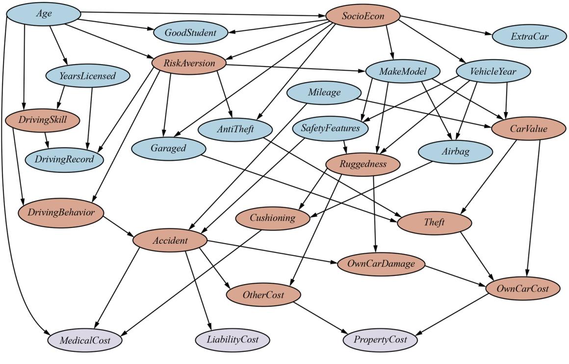
A Bayesian network for evaluating car insurance applications.

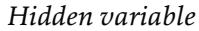
The claims to be paid out—shaded lavender in Figure 13.9 —are of three kinds: the for any injuries sustained by the applicant; the for lawsuits filed by other parties against the applicant and the company; and the for vehicle damage to either party and vehicle loss by theft. The application form asks for the following input information (the light blue nodes in Figure 13.9 ):

• About the applicant: Age; —how long since a driving license was first obtained; —some summary, perhaps based on “points,” of recent accidents and traffic violations; and (for students) a indicator for a gradepoint average of 3.0 (B) on a 4-point scale.
• About the vehicle: the and ; whether it has an ; and some summary of such as anti-lock braking and collision warning.

About the driving situation: the annual driven and how securely the vehicle is , if at all.

Now we need to think about how to arrange these into a causal structure. The key hidden variables are whether or not a or will occur in the next time period. Obviously, one cannot ask the applicant to predict these; they have to inferred from the available information and the insurer’s previous experience.

What are the causal factors leading to ? The is certainly important—some models are stolen much more often than others because there is an efficient resale market for vehicles and parts; the also matters, because an old, beat-up, or high-mileage vehicle has lower resale value. Moreover, a vehicle that is and has an device is harder to steal. The hidden variable depends in turn on the , , and . also dictates the loss amount when a occurs, so that is one of the contributors to (the other being accidents, which we will get to shortly).

It is common in models of this type to introduce another hidden variable, , the socioeconomic category of the applicant. This is thought to influence a wide range of behaviors and characteristics. In our model, there is no direct evidence in the form of observed income and occupation variables; but influences and ; it also affects and , and depends somewhat on Age. 4

4 Some insurance companies also acquire the applicant’s credit history to help in assessing risk; this provides considerably more information about socioeconomic category. Whenever using hidden variables of this kind, one must be careful that they do not inadvertently become proxies for variables such as race that may not be used in insurance decisions. Techniques for avoiding biases of this kind are described in Chapter 19 .

For any insurance company, perhaps the most important hidden variable is : people who are risk-averse are good insurance risks! Age and affect , and its “symptoms” include the applicant’s choice of whether the vehicle is and has devices and .

In predicting future accidents, the key is the applicant’s future , which is influenced by both and ; the latter in turn depends on Age and . The applicant’s past driving behavior is reflected in the , which also depends on and as well as on

(because someone who started driving only recently may not have had time to accumulate a litany of accidents and violations). In this way, provides evidence about and , which in turn help to predict future .

We can think of as a per-mile tendency to drive in an accident-prone way; whether an actually occurs in a fixed time period depends also on the annual and on the of the vehicle. If an occurs, there are three kinds of costs: the for the applicant depends on Age and , which depends in turn on the of the car and whether it has an ; the (medical, pain and suffering, loss of income, etc.) for the other driver; and the for the applicant and the other driver, both of which depend (in different ways) on the car’s and on the applicant’s .

We have illustrated the kind of reasoning that goes into developing the topology and hidden variables in a Bayes net. We also need to specify the ranges and the conditional distributions for each variable. For the ranges, the primary decision is often whether to make the variable discrete or continuous. For example, the of the vehicle could be a continuous variable between 0 and 1, or a discrete variable with range .

Continuous variables provide more precision, but they make exact inference impossible except in a few special cases. A discrete variable with many possible values can make it tedious to fill in the correspondingly large conditional probability tables and makes exact inference more expensive unless the variable’s value is always observed. For example, in a real system would have thousands of possible values, and this causes its child to have an enormous CPT that would have to be filled in from industry databases; but, because the is always observed, this does not contribute to inference complexity: in fact, the observed values for the three parents pick out exactly one relevant row of the CPT for .

The conditional distributions in the model are given in the code repository for the book; we provide a version with only discrete variables, for which exact inference can be performed. In practice, many of the variables would be continuous and the conditional distributions would be learned from historical data on applicants and their insurance claims. We will see how to learn Bayes net models from data in Chapter 20 .

The final question is, of course, how to do inference in the network to make predictions. We turn now to this question. For each inference method that we describe, we will evaluate the method on the insurance net to measure the time and space requirements of the method.

13.3 Exact Inference in Bayesian Networks

The basic task for any probabilistic inference system is to compute the posterior probability distribution for a set of query variables, given some observed event—usually, some assignment of values to a set of evidence variables. To simplify the presentation, we will consider only one query variable at a time; the algorithms can easily be extended to queries with multiple variables. (For example, we can solve the query by multiplying and .) We will use the notation from Chapter 12 : denotes the query variable; denotes the set of evidence variables , and is a particular observed event; denotes the hidden (nonevidence, nonquery) variables . Thus, the complete set of variables is . A typical query asks for the posterior probability distribution . 5

5 Another widely studied task is finding the most probable explanation for some observed evidence. This and other tasks are discussed in the notes at the end of the chapter.

Event

In the burglary network, we might observe the event in which and . We could then ask for, say, the probability that a burglary has occurred:

In this section we discuss exact algorithms for computing posterior probabilities as well as the complexity of this task. It turns out that the general case is intractable, so Section 13.4 covers methods for approximate inference.

13.3.1 Inference by enumeration

Chapter 12 explained that any conditional probability can be computed by summing terms from the full joint distribution. More specifically, a query can be answered using Equation (12.9) , which we repeat here for convenience:

\[\mathbf{P}(X|\mathbf{e}) = \alpha \,\mathbf{P}(X,\mathbf{e}) = \alpha \,\sum\_{\mathbf{y}} \mathbf{P}(X,\mathbf{e},\mathbf{y}) \,.\]

Now, a Bayes net gives a complete representation of the full joint distribution. More specifically, Equation (13.2) on page 415 shows that the terms in the joint distribution can be written as products of conditional probabilities from the network. Therefore, a query can be answered using a Bayes net by computing sums of products of conditional probabilities from the network.

Consider the query . The hidden variables for this query are Earthquake and Alarm. From Equation (12.9) , using initial letters for the variables to shorten the expressions, we have

\[\mathbf{P}(B|j,m) = \alpha \,\mathbf{P}(B,j,m) = \alpha \,\sum\_{e} \sum\_{a} \mathbf{P}(B,j,m,e,a).\]

The semantics of Bayes nets (Equation (13.2) ) then gives us an expression in terms of CPT entries. For simplicity, we do this just for :

\[\text{(13.4)}\]

\[P(b|j,m) = \alpha \sum\_{e} \sum\_{a} P(b)P(e)P(a|b,e)P(j|a)P(m|a).\]

To compute this expression, we have to add four terms, each computed by multiplying five numbers. In the worst case, where we have to sum out almost all the variables, there will be terms in the sum, each a product of probability values. A naive implementation would therefore have complexity .

This can be reduced to by taking advantage of the nested structure of the computation. In symbolic terms, this means moving the summations inwards as far as possible in expressions such as Equation (13.4) . We can do this because not all the factors in the product of probabilities depend on all the variables. Thus we have

(13.5)

\[P(b|j,m) = \alpha \, P(b) \sum\_{e} P(e) \sum\_{a} P(a|b,e) P(j|a) P(m|a)\]

This expression can be evaluated by looping through the variables in order, multiplying CPT entries as we go. For each summation, we also need to loop over the variable’s possible values. The structure of this computation is shown as a tree in Figure 13.10 . Using the numbers from Figure 13.2 , we obtain . The corresponding computation for yields ; hence,

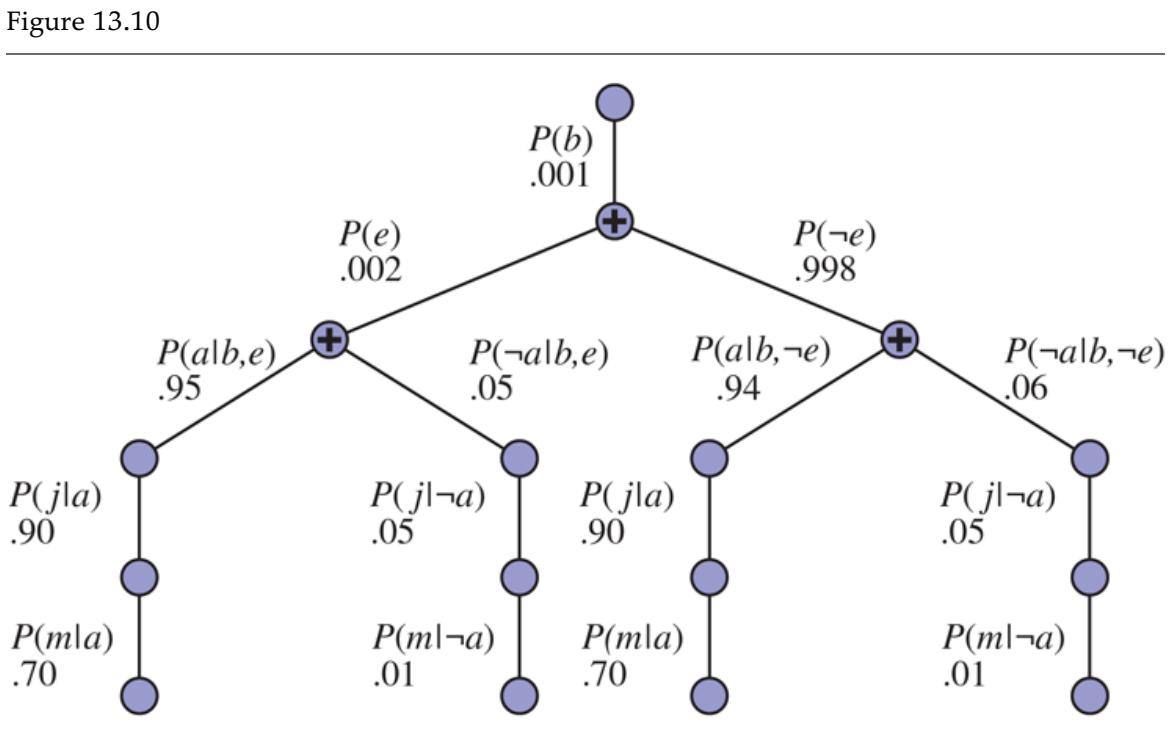
\[\mathbf{P}(B|j,m) = \alpha \langle 0.00059224, 0.0014919 \rangle \approx \langle 0.284, 0.716 \rangle.\]

The structure of the expression shown in Equation (13.5) . The evaluation proceeds top down, multiplying values along each path and summing at the ” ” nodes. Notice the repetition of the paths for and .

That is, the chance of a burglary, given calls from both neighbors, is about 28%.

The ENUMERATION-ASK algorithm in Figure 13.11 evaluates these expression trees using depth-first, left-to-right recursion. The algorithm is very similar in structure to the backtracking algorithm for solving CSPs (Figure 6.5 ) and the DPLL algorithm for satisfiability (Figure 7.17 ). Its space complexity is only linear in the number of variables: the algorithm sums over the full joint distribution without ever constructing it explicitly. Unfortunately, its time complexity for a network with Boolean variables (not counting the evidence variables) is always —better than the for the simple approach

described earlier, but still rather grim. For the insurance network in Figure 13.9 , which is relatively small, exact inference using enumeration requires around 227 million arithmetic operations for a typical query on the cost variables.

Figure 13.11

The enumeration algorithm for exact inference in Bayes nets.

If you look carefully at the tree in Figure 13.10 , however, you will see that it contains repeated subexpressions. The products and are computed twice, once for each value of . The key to efficient inference in Bayes nets is avoiding such wasted computations. The next section describes a general method for doing this.

13.3.2 The variable elimination algorithm

The enumeration algorithm can be improved substantially by eliminating repeated calculations of the kind illustrated in Figure 13.10 . The idea is simple: do the calculation once and save the results for later use. This is a form of dynamic programming. There are several versions of this approach; we present the variable elimination algorithm, which is the simplest. Variable elimination works by evaluating expressions such as Equation (13.5) in right-to-left order (that is, bottom up in Figure 13.10 ). Intermediate results are stored, and summations over each variable are done only for those portions of the expression that depend on the variable.

Variable elimination

Let us illustrate this process for the burglary network. We evaluate the expression

\[\mathbf{P}(B|j,m) = \alpha \underbrace{\mathbf{P}(B)}\_{\mathbf{f}\_1(B)} \sum\_{e} \underbrace{P(e)}\_{\mathbf{f}\_2(E)} \sum\_{a} \underbrace{\mathbf{P}(a|B,e)P(j|a)P(m|a)}\_{\mathbf{f}\_1(A,B,E)}.\]

Notice that we have annotated each part of the expression with the name of the corresponding factor; each factor is a matrix indexed by the values of its argument variables. For example, the factors and corresponding to and depend just on because and are fixed by the query. They are therefore two-element vectors:

\[\mathbf{f}\_4(A) = \begin{pmatrix} P(j|a) \\ P(j|\neg a) \end{pmatrix} = \begin{pmatrix} 0.90 \\ 0.05 \end{pmatrix} \qquad \qquad \mathbf{f}\_5(A) = \begin{pmatrix} P(m|a) \\ P(m|\neg a) \end{pmatrix} = \begin{pmatrix} 0.70 \\ 0.01 \end{pmatrix}.\]

Factor

will be a matrix, which is hard to show on the printed page. (The “first” element is given by and the “last” by .) In terms of factors, the query expression is written as

\[\mathbf{P}(B|j,m) = \alpha \mathbf{f}\_1(B) \times \sum\_e \mathbf{f}\_2(E) \times \sum\_a \mathbf{f}\_3(A,B,E) \times \mathbf{f}\_4(A) \times \mathbf{f}\_5(A).\]

Here the ” ” operator is not ordinary matrix multiplication but instead the pointwise product operation, to be described shortly.

Pointwise product

The evaluation process sums out variables (right to left) from pointwise products of factors to produce new factors, eventually yielding a factor that constitutes the solution—that is, the posterior distribution over the query variable. The steps are as follows:

First, we sum out from the product of , , and . This gives us a new factor whose indices range over just and :

\[\begin{aligned} \mathbf{f\_6}(B, E) &= \sum\_a \mathbf{f\_3}(A, B, E) \times \mathbf{f\_4}(A) \times \mathbf{f\_5}(A) \\ &= \left( \mathbf{f\_3}(a, B, E) \times \mathbf{f\_4}(a) \times \mathbf{f\_5}(a) \right) + \left( \mathbf{f\_3}(\neg a, B, E) \times \mathbf{f\_4}(\neg a) \times \mathbf{f\_5}(\neg a) \right). \end{aligned}\]

Now we are left with the expression

\[\mathbf{P}(B|j,m) = \alpha \,\mathbf{f}\_1(B) \times \sum\_{e} \mathbf{f}\_2(E) \times \mathbf{f}\_6(B,E).\]

Next, we sum out from the product of and :

\[\begin{aligned} \mathbf{f\_7}(B) &= \sum\_{e} \mathbf{f\_2}(E) \times \mathbf{f\_6}(B, E) \\ &= \mathbf{f\_2}(e) \times \mathbf{f\_6}(B, e) + \mathbf{f\_2}(\neg e) \times \mathbf{f\_6}(B, \neg e) \end{aligned}\]

This leaves the expression

\[\mathbf{P}(B|j,m) = \alpha \,\mathbf{f}\_1(B) \times \mathbf{f}\_7(B)\]

which can be evaluated by taking the pointwise product and normalizing the result.

Examining this sequence, we see that two basic computational operations are required: pointwise product of a pair of factors, and summing out a variable from a product of factors. The next section describes each of these operations.

Operations on factors

The pointwise product of two factors and yields a new factor whose variables are the union of the variables in and and whose elements are given by the product of the corresponding elements in the two factors. Suppose the two factors have variables in common. Then we have

\[\mathbf{f}(X\_1\dots X\_j, Y\_1\dots Y\_k) \times \mathbf{g}(Y\_1\dots Y\_k Z\_1,\dots Z\_\ell) = \mathbf{h}(X\_1\dots X\_j, Y\_1\dots Y\_k Z\_1\dots Z\_\ell)\]

If all the variables are binary, then and have and entries, respectively, and the pointwise product has entries. For example, given two factors and , the pointwise product has entries, as illustrated in Figure 13.12 . Notice that the factor resulting from a pointwise product can contain more variables than any of the factors being multiplied and that the size of a factor is exponential in the number of variables. This is where both space and time complexity arise in the variable elimination algorithm.

Figure 13.12

Illustrating pointwise multiplication: .

Summing out a variable from a product of factors is done by adding up the submatrices formed by fixing the variable to each of its values in turn. For example, to sum out from , we write

\[\begin{aligned} \mathbf{h}\_2(Y, Z) &= \sum\_x \mathbf{h}(X, Y, Z) = \mathbf{h}(x, Y, Z) + \mathbf{h}(\neg x, Y, Z) \\ &= \begin{pmatrix} .06 & .24 \\ .42 & .28 \end{pmatrix} + \begin{pmatrix} .18 & .72 \\ .06 & .04 \end{pmatrix} = \begin{pmatrix} .24 & .96 \\ .48 & .32 \end{pmatrix} . \end{aligned}\]

The only trick is to notice that any factor that does not depend on the variable to be summed out can be moved outside the summation. For example, to sum out from the product of and , we can move outside the summation:

\[\sum\_{x} \mathbf{f}(X, Y) \times \mathbf{g}(Y, Z) = \mathbf{g}(Y, Z) \times \sum\_{x} \mathbf{f}(X, Y).\]

This is potentially much more efficient than computing the larger pointwise product first and then summing out from that.

Notice that matrices are not multiplied until we need to sum out a variable from the accumulated product. At that point, we multiply just those matrices that include the variable to be summed out. Given functions for pointwise product and summing out, the variable elimination algorithm itself can be written quite simply, as shown in Figure 13.13 .

Figure 13.13

function ELIMINATION-ASK(X,e, bn) returns a distribution over X
inputs: X, the query variable
e, observed values for variables E
bn, a Bayesian network with variables vars
factors ←
for each V in ORDER(vars) do
factors < MAKE-FACTOR(V,e) + factors
if V is a hidden variable then factors < SUM-OUT(V,factors)
return NORMALIZE(POINTWISE-PRODUCT(factors))

The variable elimination algorithm for exact inference in Bayes nets.

Variable ordering and variable relevance

The algorithm in Figure 13.13 includes an unspecified ORDER function to choose an ordering for the variables. Every choice of ordering yields a valid algorithm, but different orderings cause different intermediate factors to be generated during the calculation. For example, in the calculation shown previously, we eliminated before ; if we do it the other way, the calculation becomes

\[\mathbf{P}(B|j,m) = \alpha \mathbf{f}\_1(B) \times \sum\_a \mathbf{f}\_4(A) \times \mathbf{f}\_5(A) \times \sum\_e \mathbf{f}\_2(E) \times \mathbf{f}\_3(A,B,E) \,,\]

during which a new factor will be generated.

In general, the time and space requirements of variable elimination are dominated by the size of the largest factor constructed during the operation of the algorithm. This in turn is determined by the order of elimination of variables and by the structure of the network. It turns out to be intractable to determine the optimal ordering, but several good heuristics are available. One fairly effective method is a greedy one: eliminate whichever variable minimizes the size of the next factor to be constructed.

Let us consider one more query: . As usual (see Equation (13.5) ), the first step is to write out the nested summation:

\[\mathbf{P}(J|b) = \alpha \, P(b) \sum\_{e} P(e) \sum\_{a} P(a|b, e) \mathbf{P}(J|a) \sum\_{m} P(m|a) .\]

Evaluating this expression from right to left, we notice something interesting: is equal to 1 by definition! Hence, there was no need to include it in the first place; the variable is irrelevant to this query. Another way of saying this is that the result of the query is unchanged if we remove from the network altogether. In general, we can remove any leaf node that is not a query variable or an evidence variable. After its removal, there may be some more leaf nodes, and these too may be irrelevant. Continuing this process, we eventually find that every variable that is not an ancestor of a query variable or evidence variable is irrelevant to the query. A variable elimination algorithm can therefore remove all these variables before evaluating the query.

When applied to the insurance network shown in Figure 13.9 , variable elimination shows considerable improvement over the naive enumeration algorithm. Using reverse topological order for the variables, exact inference using elimination is about 1,000 times faster than the enumeration algorithm.

13.3.3 The complexity of exact inference

The complexity of exact inference in Bayes nets depends strongly on the structure of the network. The burglary network of Figure 13.2 belongs to the family of networks in which there is at most one undirected path (i.e., ignoring the direction of the arrows) between any two nodes in the network. These are called singly connected networks or polytrees, and they have a particularly nice property: The time and space complexity of exact inference in polytrees is linear in the size of the network. Here, the size is defined as the number of CPT entries; if the number of parents of each node is bounded by a constant, then the complexity will also be linear in the number of nodes. These results hold for any ordering consistent with the topological ordering of the network (Exercise 13.VEEX).

Singly connected

Polytree

For multiply connected networks, such as the insurance network in Figure 13.9 , variable elimination can have exponential time and space complexity in the worst case, even when the number of parents per node is bounded. This is not surprising when one considers that because it includes inference in propositional logic as a special case, inference in Bayes nets is NPhard. To prove this, we need to work out how to encode a propositional satisfiability problem as a Bayes net, such that running inference on this net tells us whether or not the original propositional sentences are satisfiable. (In the language of complexity theory, we reduce satisfiability problems to Bayes net inference problems.) This turns out to be quite straightforward. Figure 13.14 shows how to encode a particular 3-SAT problem. The propositional variables become the root variables of the network, each with prior probability 0.5. The next layer of nodes corresponds to the clauses, with each clause variable connected to the appropriate variables as parents. The conditional distribution for a clause variable is a deterministic disjunction, with negation as needed, so that each clause variable is true if and only if the assignment to its parents satisfies that clause. Finally, is the conjunction of the clause variables.

Figure 13.14

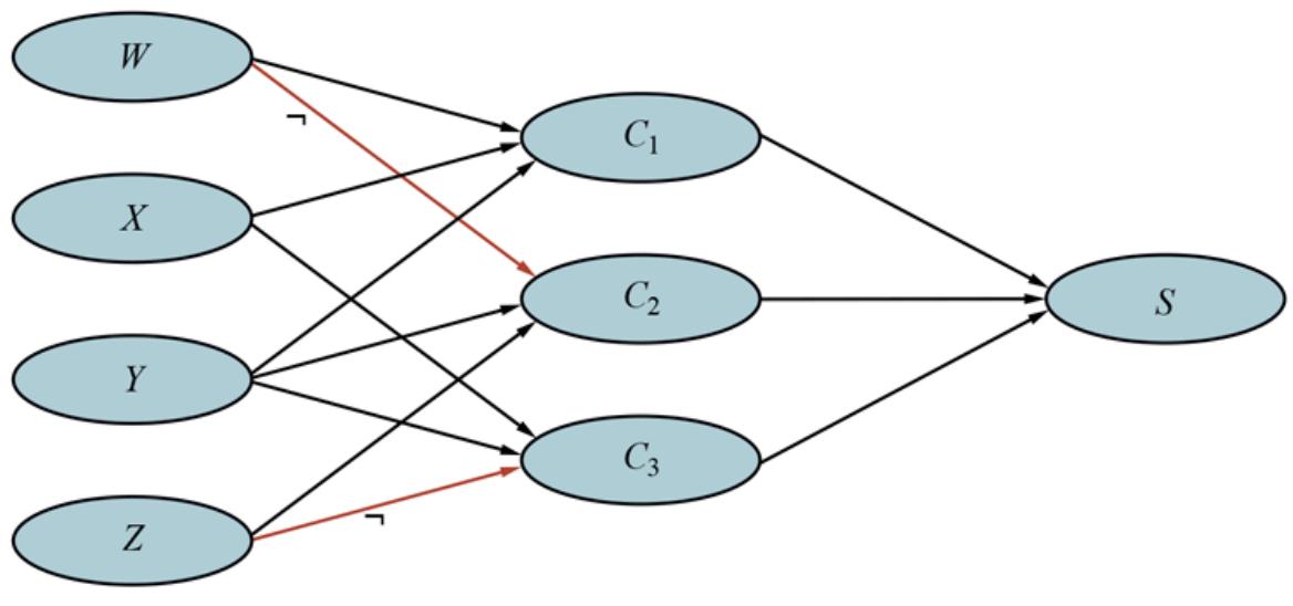
Bayes net encoding of the 3-CNF sentence

Multiply connected

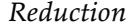
To determine if the original sentence is satisfiable, we simply evaluate . If the sentence is satisfiable, then there is some possible assignment to the logical variables that makes true; in the Bayes net, this means that there is possible world with nonzero probability in which the root variables have that assignment, the clause variables have value true, and has value true. Therefore, for a satisfiable sentence. Conversely, for an unsatisfiable sentence: all worlds with have probability 0. Hence, we can use Bayes net inference to solve 3-SAT problems; from this, we conclude that Bayes net inference is NP-hard.

We can, in fact, do more than this. Notice that the probability of each satisfying assignment is for a problem with variables. Hence, the number of satisfying assignments is . Because computing the number of satisfying assignments for a 3-SAT

problem is #P-complete (“number-P complete”), this means that Bayes net inference is #Phard—that is, strictly harder than NP-complete problems.

There is a close connection between the complexity of Bayes net inference and the complexity of constraint satisfaction problems (CSPs). As we discussed in Chapter 6 , the difficulty of solving a discrete CSP is related to how “treelike” its constraint graph is. Measures such as tree width, which bound the complexity of solving a CSP, can also be applied directly to Bayes nets. Moreover, the variable elimination algorithm can be generalized to solve CSPs as well as Bayes nets.

As well as reducing satisfiability problems to Bayes net inference, we can reduce Bayes net inference to satisfiability, which allows us to take advantage of the powerful machinery developed for SAT-solving (see Chapter 7 ). In this case, the reduction is to a particular form of SAT solving called weighted model counting (WMC). Regular model counting counts the number of satisfying assignments for a SAT expression; WMC sums the total weight of those satisfying assignments—where, in this application, the weight is essentially the product of the conditional probabilities for each variable assignment given its parents. (See Exercise 13.WMCX for details.) Partly because SAT-solving technology has been so well optimized for large-scale applications, Bayes net inference via WMC is competitive with and sometimes superior to other exact algorithms on networks with large tree width.

Weighted model counting

13.3.4 Clustering algorithms

The variable elimination algorithm is simple and efficient for answering individual queries. If we want to compute posterior probabilities for all the variables in a network, however, it can be less efficient. For example, in a polytree network, one would need to issue queries costing each, for a total of time. Using clustering algorithms (also known as join tree algorithms), the time can be reduced to . For this reason, these algorithms are widely used in commercial Bayes net tools.

Join tree

The basic idea of clustering is to join individual nodes of the network to form cluster nodes in such a way that the resulting network is a polytree. For example, the multiply connected network shown in Figure 13.15(a) can be converted into a polytree by combining the Sprinkler and Rain node into a cluster node called , as shown in Figure 13.15(b) . The two Boolean nodes are replaced by a meganode that takes on four possible values: , , , and . The meganode has only one parent, the Boolean variable Cloudy, so there are two conditioning cases. Although this example doesn’t show it, the process of clustering often produces meganodes that share some variables.

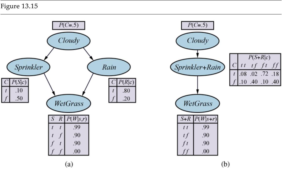
1. A multiply connected network describing Mary’s daily lawn routine: each morning, she checks the weather; if it’s cloudy, she usually doesn’t turn on the sprinkler; if the sprinkler is on, or if it rains during the day, the grass will be wet. Thus, Cloudy affects WetGrass via two different causal pathways. (b) A clustered equivalent of the multiply connected network.

Meganode

Once the network is in polytree form, a special-purpose inference algorithm is required, because ordinary inference methods cannot handle meganodes that share variables with each other. Essentially, the algorithm is a form of constraint propagation (see Chapter 6 ) where the constraints ensure that neighboring meganodes agree on the posterior probability of any variables that they have in common. With careful bookkeeping, this algorithm is able to compute posterior probabilities for all the nonevidence nodes in the network in time linear in the size of the clustered network. However, the NP-hardness of the problem has not disappeared: if a network requires exponential time and space with variable elimination, then the CPTs in the clustered network will necessarily be exponentially large.

13.4 Approximate Inference for Bayesian Networks

Given the intractability of exact inference in large networks, we will now consider approximate inference methods. This section describes randomized sampling algorithms, also called Monte Carlo algorithms, that provide approximate answers whose accuracy depends on the number of samples generated. They work by generating random events based on the probabilities in the Bayes net and counting up the different answers found in those random events. With enough samples, we can get arbitrarily close to recovering the true probability distribution—provided the Bayes net has no deterministic conditional distributions.

Monte Carlo

Monte Carlo algorithms, of which simulated annealing (page 115) is an example, are used in many branches of science to estimate quantities that are difficult to calculate exactly. In this section, we are interested in sampling applied to the computation of posterior probabilities in Bayes nets. We describe two families of algorithms: direct sampling and Markov chain sampling. Several other approaches for approximate inference are mentioned in the notes at the end of the chapter.

13.4.1 Direct sampling methods

The primitive element in any sampling algorithm is the generation of samples from a known probability distribution. For example, an unbiased coin can be thought of as a random variable with values and a prior distribution . Sampling from this distribution is exactly like flipping the coin: with probability 0.5 it will return , and with probability 0.5 it will return . Given a source of random numbers uniformly distributed in the range , it is a simple matter to sample any distribution on a single variable, whether discrete or continuous. This is done by constructing the cumulative distribution for the variable and returning the first value whose cumulative probability exceeds (see Exercise 13.PRSA).

We begin with a random sampling process for a Bayes net that has no evidence associated with it. The idea is to sample each variable in turn, in topological order. The probability distribution from which the value is sampled is conditioned on the values already assigned to the variable’s parents. (Because we sample in topological order, the parents are guaranteed to have values already.) This algorithm is shown in Figure 13.16 . Applying it to the network in Figure 13.15(a) with the ordering Cloudy, Sprinkler, Rain, WetGrass, we might produce a random event as follows:

• 1. Sample from , value is true.
• 2. Sample from , value is false.
• 3. Sample from , value is true.
• 4. Sample from , value is true.

Figure 13.16

A sampling algorithm that generates events from a Bayesian network. Each variable is sampled according to the conditional distribution given the values already sampled for the variable’s parents.

In this case, PRIOR-SAMPLE returns the event .

It is easy to see that PRIOR-SAMPLE generates samples from the prior joint distribution specified by the network. First, let be the probability that a specific event is generated by the PRIOR-SAMPLE algorithm. Just looking at the sampling process, we have

\[S\_{PS}(x\_1, \ldots, x\_n) = \prod\_{i=1}^n P(x\_i |parent(X\_i))\]

because each sampling step depends only on the parent values. This expression should look familiar, because it is also the probability of the event according to the Bayesian net’s representation of the joint distribution, as stated in Equation (13.2) . That is, we have

\[S\_{PS}(x\_1 \ldots x\_n) = P(x\_1 \ldots x\_n).\]

This simple fact makes it easy to answer questions by using samples.

In any sampling algorithm, the answers are computed by counting the actual samples generated. Suppose there are total samples produced by the PRIOR-SAMPLE algorithm, and let be the number of times the specific event occurs in the set of samples. We expect this number, as a fraction of the total, to converge in the limit to its expected value according to the sampling probability:

(13.6)

\[\lim\_{N \to \infty} \frac{N\_{PS}(x\_1, \dots, x\_n)}{N} = S\_{PS}(x\_1, \dots, x\_n) = P(x\_1, \dots, x\_n).\]

For example, consider the event produced earlier: . The sampling probability for this event is

\[S\_{PS}(true,false,true,true) = 0.5 \times 0.9 \times 0.8 \times 0.9 = 0.324...\]

Hence, in the limit of large , we expect 32.4% of the samples to be of this event.

Whenever we use an approximate equality (” “) in what follows, we mean it in exactly this sense—that the estimated probability becomes exact in the large-sample limit. Such an estimate is called consistent. For example, one can produce a consistent estimate of the probability of any partially specified event , where , as follows:

(13.7)

\[P(x\_1, \ldots, x\_m) \approx N\_{PS}(x\_1, \ldots, x\_m) / N.\]

Consistent

That is, the probability of the event can be estimated as the fraction of all complete events generated by the sampling process that match the partially specified event. We will use

(pronounced “P-hat”) to mean an estimated probability. So, if we generate 1,000 samples from the sprinkler network, and 511 of them have , then the estimated probability of rain is .

Rejection sampling in Bayesian networks

Rejection sampling is a general method for producing samples from a hard-to-sample distribution given an easy-to-sample distribution. In its simplest form, it can be used to compute conditional probabilities—that is, to determine . The REJECTION-SAMPLING algorithm is shown in Figure 13.17 . First, it generates samples from the prior distribution specified by the network. Then, it rejects all those that do not match the evidence. Finally, the estimate is obtained by counting how often occurs in the remaining samples.

Figure 13.17

The rejection-sampling algorithm for answering queries given evidence in a Bayesian network.

Rejection sampling

Let be the estimated distribution that the algorithm returns; this distribution is computed by normalizing , the vector of sample counts for each value of where the sample agrees with the evidence :

\[ \hat{\mathbf{P}}(X|\mathbf{e}) = \alpha \,\mathbf{N}\_{PS}(X,\mathbf{e}) = \frac{\mathbf{N}\_{PS}(X,\mathbf{e})}{N\_{PS}(\mathbf{e})}. \]

From Equation (13.7) , this becomes

\[ \hat{\mathbf{P}}(X|\mathbf{e}) \approx \frac{\mathbf{P}(X, \mathbf{e})}{P(\mathbf{e})} = \mathbf{P}(X|\mathbf{e}). \]

That is, rejection sampling produces a consistent estimate of the true probability.

Continuing with our example from Figure 13.15(a) , let us assume that we wish to estimate , using 100 samples. Of the 100 that we generate, suppose that 73 have and are rejected, while 27 have ; of the 27, 8 have and 19 have . Hence,

\(\mathbf{P}(Rain|Sprinkler = true) \approx \text{NORMizz}\) \((\langle \, 8, 19 \rangle) = \langle 0.296, 0.704 \rangle\) .

The true answer is . As more samples are collected, the estimate will converge to the true answer. The standard deviation of the error in each probability will be proportional to , where is the number of samples used in the estimate.

Now we know that rejection sampling converges to the correct answer, the next question is, how fast does that happen? More precisely, how many samples are required before we know that the resulting estimates are close to the correct answers with high probability? Whereas the complexity of exact algorithms depends to a large extent on the topology of the network—trees are easy, densely connected networks are hard—the complexity of rejection sampling depends primarily on the fraction of samples that are accepted. This fraction is exactly equal to the prior probability of the evidence, . Unfortunately, for complex problems with many evidence variables, this fraction is vanishingly small. When applied to the discrete version of the car insurance network in Figure 13.9 , the fraction of samples consistent with a typical evidence case sampled from the network itself is usually between one in a thousand and one in ten thousand. Convergence is extremely slow (see Figure 13.19 below).

We expect the fraction of samples consistent with the evidence to drop exponentially as the number of evidence variables grows, so the procedure is unusable for complex problems. It also has difficulties with continuous-valued evidence variables, because the

probability of producing a sample consistent with such evidence is zero (if it is really continuous-valued) or infinitesimal (if it is merely a finite-precision floating-point number).

Notice that rejection sampling is very similar to the estimation of conditional probabilities in the real world. For example, to estimate the conditional probability that any humans survive after a 1km-diameter asteroid crashes into the Earth, one can simply count how often any humans survive after a 1km-diameter asteroid crashes into the Earth, ignoring all those days when no such event occurs. (Here, the universe itself plays the role of the samplegeneration algorithm.) To get a decent estimate, one might need to wait for 100 such events to occur. Obviously, this could take a long time, and that is the weakness of rejection sampling.

Importance sampling

The general statistical technique of importance sampling aims to emulate the effect of sampling from a distribution using samples from another distribution . We ensure that the answers are correct in the limit by applying a correction factor , also known as a weight, to each sample when counting up the samples.

Importance sampling

The reason for using importance sampling in Bayes nets is simple: we would like to sample from the true posterior distribution conditioned on all the evidence, but usually this is too hard; so instead, we sample from an easy distribution and apply the necessary corrections. The reason why importance sampling works is also simple. Let the nonevidence variables be . If we could sample directly from , we could construct estimates like this: 6

6 If it was easy, then we could approximate the desired probability to arbitrary accuracy with a polynomial number of samples. It can be shown that no such polynomial-time approximation scheme can exist.

\[ \hat{P}(\mathbf{z}|\mathbf{e}) = \frac{N\_P(\mathbf{z})}{N} \approx P(\mathbf{z}|\mathbf{e}) \]

where is the number of samples with when sampling from . Now suppose instead that we sample from . The estimate in this case includes the correction factors:

\[ \hat{P}(\mathbf{z}|\mathbf{e}) = \frac{N\_Q(\mathbf{z})}{N} \frac{P(\mathbf{z}|\mathbf{e})}{Q(\mathbf{z})} \approx Q(\mathbf{z}) \frac{P(\mathbf{z}|\mathbf{e})}{Q(\mathbf{z})} = P(\mathbf{z}|\mathbf{e}). \]

Thus, the estimate converges to the correct value regardless of which sampling distribution is used. (The only technical requirement is that should not be zero for any where is nonzero.) Intuitively, the correction factor compensates for oversampling or undersampling. For example, if is much bigger than for some , then there will be many more samples of that than there should be, but each will have a small weight, so it works out just as if there were the right number.

As for which to use, we want one that is easy to sample from and as close as possible to the true posterior . The most common approach is called likelihood weighting (for reasons we will see shortly). As shown in the WEIGHTED-SAMPLE function in Figure 13.18 , the algorithm fixes the values for the evidence variables and samples all the nonevidence variables in topological order, each conditioned on its parents. This guarantees that each event generated is consistent with the evidence.

Figure 13.18

function LIKELIHOOD-WEIGHTING(X,e, bn, N) returns an estimate of P(X e) inputs: X, the query variable e, observed values for variables E bn, a Bayesian network specifying joint distribution P(X1, , Xn) N, the total number of samples to be generated local variables: W, a vector of weighted counts for each value of X, initially zero
for j = 1 to N do x, w < WEIGHTED-SAMPLE(bn,e) W[j] < W[j] + w where x ; is the value of X in x return NORMALIZE(W)
function WEIGHTED-SAMPLE(bn,e) returns an event and a weight
w < 1; x < an event with n elements, with values fixed from e for i = 1 to n do if X; is an evidence variable with value xij in e then w < w x P(X;= xij parents(Xi)) else x i < a random sample from P(X; parents(Xi))

The likelihood-weighting algorithm for inference in Bayesian networks. In WEIGHTED-SAMPLE, each nonevidence variable is sampled according to the conditional distribution given the values already sampled for the variable’s parents, while a weight is accumulated based on the likelihood for each evidence variable.

Likelihood weighting

Let’s call the sampling distribution produced by this algorithm . If the nonevidence variables are , then we have

(13.8)

\[Q\_{WS}(\mathbf{z}) = \prod\_{i=1}^{l} P(z\_i |parents(Z\_i))\]

because each variable is sampled conditioned on its parents. In order to complete the algorithm, we need to know how to compute the weight for each sample generated from . According to the general scheme for importance sampling, the weight should be

\[w(\mathbf{z}) = P(\mathbf{z}|\mathbf{e}) / Q\_{WS}(\mathbf{z}) = \alpha P(\mathbf{z}, \mathbf{e}) / Q\_{WS}(\mathbf{z})\]

where the normalizing factor is the same for all samples. Now and together cover all the variables in the Bayes net, so is just the product of all the conditional probabilities (Equation (13.2) page 415); and we can write this as the product of the conditional probabilities for the nonevidence variables times the product of the conditional probabilities for the evidence variables:

(13.9)

\[w(\mathbf{z}) = \alpha \frac{P(\mathbf{z}, \mathbf{e})}{Q\_{WS}(\mathbf{z})} = \alpha \frac{\prod\_{i=1}^{l} P(z\_i |parents(Z\_i)) \prod\_{i=1}^{m} P(e\_i |parents(E\_i))}{\prod\_{i=1}^{l} P(z\_i |parents(Z\_i))}\]

\[= \alpha \prod\_{i=1}^{m} P(e\_i |parents(E\_i)).\]

Thus the weight is the product of the conditional probabilities for the evidence variables given their parents. (Probabilities of evidence are generally called likelihoods, hence the name.) The weight calculation is implemented incrementally in WEIGHTED-SAMPLE, multiplying by the conditional probability each time an evidence variable is encountered. The normalization is done at the end before the query result is returned.

Let us apply the algorithm to the network shown in Figure 13.15(a) , with the query and the ordering Cloudy, Sprinkler, Rain, WetGrass. (Any topological ordering will do.) The process goes as follows: First, the weight is set to 1.0. Then an event is generated:

1. Cloudy is an evidence variable with value true. Therefore, we set

\[w \gets w \times P(Cloudy = true) = 0.5\]

• 2. Sprinkler is not an evidence variable, so sample from ; suppose this returns false.
• 3. Rain is not an evidence variable, so sample from ; suppose this returns true.
• 4. WetGrass is an evidence variable with value true. Therefore, we set

\[\begin{aligned} w &\leftarrow & w \times P(WetGross = true | Sprinkler = false, Rain = true) \\ &= & 0.5 \times 0.9 = 0.45. \end{aligned}\]

Here WEIGHTED-SAMPLE returns the event with weight 0.45, and this is tallied under .

Notice that can include both nonevidence variables and evidence variables. Unlike the prior distribution , the distribution pays some attention to the evidence: the sampled values for each will be influenced by evidence among ’s ancestors. For example, when sampling Sprinkler the algorithm pays attention to the evidence in its parent variable. On the other hand, pays less attention to the evidence than does the true posterior distribution , because the sampled values for each ignore evidence among ’s non-ancestors. For example, when sampling Sprinkler and Rain the algorithm ignores the evidence in the child variable ; this means it will generate many samples with and despite the fact that the evidence actually rules out this case. Those samples will have zero weight.

Because likelihood weighting uses all the samples generated, it can be much more efficient than rejection sampling. It will, however, suffer a degradation in performance as the number of evidence variables increases. This is because most samples will have very low weights and hence the weighted estimate will be dominated by the tiny fraction of samples that

accord more than an infinitesimal likelihood to the evidence. The problem is exacerbated if the evidence variables occur “downstream”—that is, late in the variable ordering—because then the nonevidence variables will have no evidence in their parents and ancestors to guide the generation of samples. This means the samples will be mere hallucinations simulations that bear little resemblance to the reality suggested by the evidence.

When applied to the discrete version of the car insurance network in Figure 13.9 , likelihood weighting is considerably more efficient than rejection sampling (see Figure 13.19 ). The insurance network is a relatively benign case for likelihood weighting because much of the evidence is “upstream” and the query variables are leaf nodes of the network.

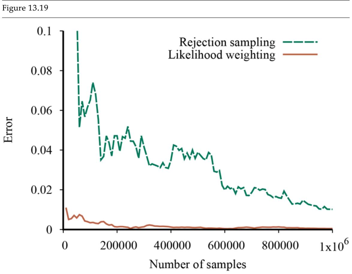
Performance of rejection sampling and likelihood weighting on the insurance network. The x-axis shows the number of samples generated and the y-axis shows the maximum absolute error in any of the probability values for a query on .

13.4.2 Inference by Markov chain simulation

Markov chain Monte Carlo (MCMC) algorithms work differently from rejection sampling and likelihood weighting. Instead of generating each sample from scratch, MCMC algorithms generate a sample by making a random change to the preceding sample. Think of an MCMC algorithm as being in a particular current state that specifies a value for every variable and generating a next state by making random changes to the current state.

Markov chain Monte Carlo

The term Markov chain refers to a random process that generates a sequence of states. (Markov chains also figure prominently in Chapters 14 and 17 ; the simulated annealing algorithm in Chapter 4 and the WALKSAT algorithm in Chapter 7 are also members of the MCMC family.) We begin by describing a particular form of MCMC called Gibbs sampling, which is especially well suited for Bayes nets. We then describe the more general Metropolis–Hastings algorithm, which allows much greater flexibility in generating samples.

Markov chain

Gibbs sampling

Metropolis–Hastings

Gibbs sampling in Bayesian networks

The Gibbs sampling algorithm for Bayesian networks starts with an arbitrary state (with the evidence variables fixed at their observed values) and generates a next state by randomly

sampling a value for one of the nonevidence variables . Recall from page 419 that is independent of all other variables given its Markov blanket (its parents, children, and children’s other parents); therefore, Gibbs sampling for means sampling conditioned on the current values of the variables in its Markov blanket. The algorithm wanders randomly around the state space—the space of possible complete assignments—flipping one variable at a time, but keeping the evidence variables fixed. The complete algorithm is shown in Figure 13.20 .

Figure 13.20
————–	–	–

The Gibbs sampling algorithm for approximate inference in Bayes nets; this version chooses variables at random, but cycling through the variables but also works.

Consider the query for the network in Figure 13.15(a) . The evidence variables Sprinkler and WetGrass are fixed to their observed values (both true), and the nonevidence variables Cloudy and Rain are initialized randomly to, say, true and false respectively. Thus, the initial state is , where we have marked the fixed evidence values in bold. Now the nonevidence variables are sampled repeatedly in some random order according to a probability distribution for choosing variables. For example:

• 1. Cloudy is chosen and then sampled, given the current values of its Markov blanket: in this case, we sample from . Suppose the result is . Then the new current state is .
• 2. Rain is chosen and then sampled, given the current values of its Markov blanket: in this case, we sample from

. Suppose this yields . The new current state is .

The one remaining detail concerns the method of calculating the Markov blanket distribution , where denotes the values of the variables in ’s Markov blanket, . Fortunately, this does not involves any complex inference. As shown in Exercise 13.MARB, the distribution is given by

(13.10)

\[P(x\_i|mb(X\_i)) = \alpha \, P(x\_i|parents(X\_i)) \prod\_{Y\_j \in Chilrend(X\_i)} P(y\_j|parents(Y\_j)).\]

In other words, for each value , the probability is given by multiplying probabilities from the CPTs of and its children. For example, in the first sampling step shown above, we sampled from . By Equation (13.10) , and abbreviating the variable names, we have

\[\begin{aligned} P(c|s,\neg r) &=& \alpha \, P(c)P(s|c)P(\neg r|c) = \alpha \, 0.5 \cdot 0.1 \cdot 0.2\\ P(\neg c|s,\neg r) &=& \alpha \, P(\neg c)P(s|\neg c)P(\neg r|\neg c) = \alpha \, 0.5 \cdot 0.5 \cdot 0.8, \end{aligned}\]

so the sampling distribution is .

Figure 13.21(a) shows the complete Markov chain for the case where variables are chosen uniformly, i.e., . The algorithm is simply wandering around in this graph, following links with the stated probabilities. Each state visited during this process is a sample that contributes to the estimate for the query variable Rain. If the process visits 20 states where Rain is true and 60 states where Rain is false, then the answer to the query is .

Figure 13.21

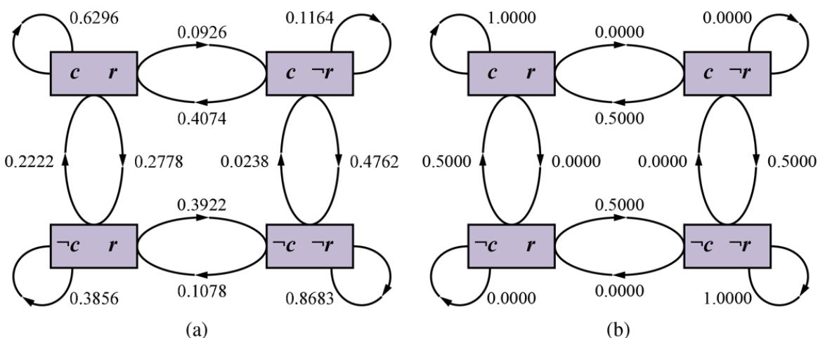
1. The states and transition probabilities of the Markov chain for the query . Note the self-loops: the state stays the same when either variable is chosen and then resamples the same value it already has. (b) The transition probabilities when the CPT for Rain constrains it to have the same value as Cloudy.

Analysis of Markov chains

We have said that Gibbs sampling works by wandering randomly around the state space to generate samples. To explain why Gibbs sampling works correctly—that is, why its estimates converge to correct values in the limit—we will need some careful analysis. (This section is somewhat mathematical and can be skipped on first reading.)

We begin with some of the basic concepts for analyzing Markov chains in general. Any such chain is defined by its initial state and its transition kernel —the probability of a transition to state starting from state . Now suppose that we run the Markov chain for steps, and let be the probability that the system is in state at time . Similarly, let be the probability of being in state at time . Given , we can calculate by summing, for all states the system could be in at time , the probability of being in times the probability of making the transition to :

\[ \pi\_{t+1}(\mathbf{x}') = \sum\_{\mathbf{x}} \pi\_t(\mathbf{x}) k(\mathbf{x} \to \mathbf{x}'). \]

Transition kernel

We say that the chain has reached its stationary distribution if . Let us call this stationary distribution ; its defining equation is therefore

(13.11)

\[ \pi(\mathbf{x'}) = \sum\_{\mathbf{x}} \pi(\mathbf{x}) k(\mathbf{x} \to \mathbf{x'}) \qquad \text{for all } \mathbf{x'}. \]

Stationary distribution

Provided the transition kernel is ergodic—that is, every state is reachable from every other and there are no strictly periodic cycles—there is exactly one distribution satisfying this equation for any given .

Ergodic

Equation (13.11) can be read as saying that the expected “outflow” from each state (i.e., its current “population”) is equal to the expected “inflow” from all the states. One obvious way to satisfy this relationship is if the expected flow between any pair of states is the same in both directions; that is,

(13.12)

\[ \pi(\mathbf{x})k(\mathbf{x}\to\mathbf{x'}) = \pi(\mathbf{x'})k(\mathbf{x'}\to\mathbf{x})\qquad\text{for all }\mathbf{x},\mathbf{x'}. \]

When these equations hold, we say that is in detailed balance with . One special case is the self-loop , i.e., a transition from a state to itself. In that case, the detailed balance condition becomes which is of course trivially true for any stationary distribution and any transition kernel .

We can show that detailed balance implies stationarity simply by summing over in Equation (13.12) . We have

\[\sum\_{\mathbf{x}} \pi(\mathbf{x}) k(\mathbf{x} \to \mathbf{x}') = \sum\_{\mathbf{x}} \pi(\mathbf{x}') k(\mathbf{x}' \to \mathbf{x}) = \pi(\mathbf{x}') \sum\_{\mathbf{x}} k(\mathbf{x}' \to \mathbf{x}) = \pi(\mathbf{x}')\]

where the last step follows because a transition from is guaranteed to occur.

Why Gibbs sampling works

We will now show that Gibbs sampling returns consistent estimates for posterior probabilities. The basic claim is straightforward: the stationary distribution of the Gibbs sampling process is exactly the posterior distribution for the nonevidence variables conditioned on the evidence. This remarkable property follows from the specific way in which the Gibbs sampling process moves from state to state.

The general definition of Gibbs sampling is that a variable is chosen and then sampled conditionally on the current values of all the other variables. (When applied specifically to Bayes nets, we simply use the additional fact that sampling conditionally on all variables is equivalent to sampling conditionally on the variable’s Markov blanket, as shown on page 419.) We will use the notation to refer to these other variables (except the evidence variables); their values in the current state are .

To write down the transition kernel for Gibbs sampling, there are three cases to consider:

• 1. The states and differ in two or more variables. In that case, because Gibbs sampling changes only a single variable.
• 2. The states differ in exactly one variable that changes its value from to . The probability of such an occurrence is (13.13)

\[k(\mathbf{x} \rightarrow \mathbf{x}') = k((x\_i, \overline{\mathbf{x}\_i}) \rightarrow (x'\_i, \overline{\mathbf{x}\_i})) = \rho(i) P(x'\_i | \overline{\mathbf{x}\_i}).\]

3. The states are the same: . In that case, any variable could be chosen but then the sampling process produces the same value the variable already has. The probability of such an occurrence is

\[k(\mathbf{x}\rightarrow\mathbf{x}) = \sum\_{i} \rho(i)k((x\_i,\overline{\mathbf{x}\_i})\rightarrow(x\_i,\overline{\mathbf{x}\_i})) = \sum\_{i} \rho(i)P(x\_i|\overline{\mathbf{x}\_i}).\]

Now we show that this general definition of Gibbs sampling satisfies the detailed balance equation with a stationary distribution equal to , the true posterior distribution on the nonevidence variables. That is, we show that where , for all states and .

For the first and third cases given above, detailed balance is always satisfied: if two states differ in two or more variables, the transition probability in both directions is zero. If then from Equation (13.13) , we have

\[\begin{aligned} &\pi(\mathbf{x})k(\mathbf{x}\rightarrow\mathbf{x}') = P(\mathbf{x}|\mathbf{e})\rho(i)P(x\_i'|\overline{\mathbf{x}\_i},\mathbf{e}) = \rho(i)P(x\_i;\overline{\mathbf{x}\_i}|\mathbf{e})P(x\_i'|\overline{\mathbf{x}\_i},\mathbf{e})\\ &= \rho(i)P(x\_i|\overline{\mathbf{x}\_i},\mathbf{e})P(\overline{\mathbf{x}\_i}|\mathbf{e})P(x\_i'|\overline{\mathbf{x}\_i},\mathbf{e}) \quad \text{(using the chain rule on the first term)}\\ &= \rho(i)P(x\_i|\overline{\mathbf{x}\_i},\mathbf{e})P(x\_i',\overline{\mathbf{x}\_i}|\mathbf{e}) \quad \text{(reverse chain rule on last two terms)}\\ &= \pi(\mathbf{x}')k(\mathbf{x}' \rightarrow \mathbf{x}). \end{aligned}\]

The final piece of the puzzle is the ergodicity of the chain—that is, every state must be reachable from every other and there are no periodic cycles. Both conditions are satisfied provided the CPTs do not contain probabilities of 0 or 1. Reachability comes from the fact that we can convert one state into another by changing one variable at a time, and the absence of periodic cycles comes from the fact that every state has a self-loop with nonzero probability. Hence, under the stated conditions, is ergodic, which means that the samples generated by Gibbs sampling will eventually be drawn from the true posterior distribution.

Complexity of Gibbs sampling

First, the good news: each Gibbs sampling step involves calculating the Markov blanket distribution for the chosen variable , which requires a number of multiplications proportional to the number of ’s children and the size of ’s range. This is important because it means that the work required to generate each sample is independent of the size of the network.

Now, the not necessarily bad news: the complexity of Gibbs sampling is much harder to analyze than that of rejection sampling and likelihood weighting. The first thing to notice is that Gibbs sampling, unlike likelihood weighting, does pay attention to downstream evidence. Information propagates from evidence nodes in all directions: first, any neighbors of the evidence nodes sample values that reflect the evidence in those nodes; then their neighbors, and so on. Thus, we expect Gibbs sampling to outperform likelihood weighting when evidence is mostly downstream; and indeed, this is borne out in Figure 13.22 .

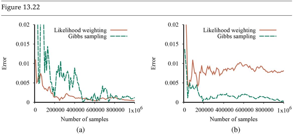
Performance of Gibbs sampling compared to likelihood weighting on the car insurance network: (a) for the standard query on , and (b) for the case where the output variables are observed and Age is the query variable.

The rate of convergence for Gibbs sampling—the mixing rate of the Markov chain defined by the algorithm—depends strongly on the quantitative properties of the conditional distributions in the network. To see this, consider what happens in Figure 13.15(a) as the CPT for Rain becomes deterministic: it rains if and only if it is cloudy. In that case, the true posterior distribution for the query is roughly but Gibbs sampling will never reach this value. The problem is that the only two joint states for Cloudy and Rain that have non-zero probability are and . Starting in , the chain can never reach because transitions to the intermediate states have probability zero (see Figure 13.21(b) ). So, if the process starts in it always reports a posterior probability for the query of ; if it starts in it always reports a posterior probability for the query of .

Mixing rate

Gibbs sampling fails in this case because the deterministic relationship between Cloudy and Rain breaks the property of ergodicity that is required for convergence. If, however, we make the relationship nearly deterministic, then convergence is restored, but happens arbitrarily slowly. There are several fixes that help MCMC algorithms mix more quickly. One is block sampling: sampling multiple variables simultaneously. In this case, we could sample Cloudy and Rain jointly, conditioned on their combined Markov blanket. Another is to generate next states more intelligently, as we will see in the next section.

Block sampling

Metropolis–Hastings sampling

.

The Metropolis–Hastings or MH sampling method is perhaps the most broadly applicable MCMC algorithm. Like Gibbs sampling, MH is designed to generate samples (eventually) according to target probabilities ; in the case of inference in Bayesian networks, we want .) Like simulated annealing (page 115), MH has two stages in each iteration of the sampling process:

1. Sample a new state from a proposal distribution , given the current state

Proposal distribution

2. Probabilistically accept or reject according to the acceptance probability

\[a(\mathbf{x'}|\mathbf{x}) = \min\left(1, \frac{\pi(\mathbf{x'})q(\mathbf{x}|\mathbf{x'})}{\pi(\mathbf{x})q(\mathbf{x'}|\mathbf{x})}\right).\]

Acceptance probability

If the proposal is rejected, the state remains at .

The transition kernel for MH consists of this two-step process. Note that if the proposal is rejected, the chain stays in the same state.

The proposal distribution is responsible, as its name suggests, for proposing a next state . For example, could be defined as follows:

• With probability 0.95, perform a Gibbs sampling step to generate .
• Otherwise, generate by running the WEIGHTED-SAMPLE algorithm from page 440.

This proposal distribution causes MH to do about 20 steps of Gibbs sampling then “restarts” the process from a new state (assuming it is accepted) that is generated from scratch. By this stratagem, it gets around the problem of Gibbs sampling getting stuck in one part of the state space and being unable to reach the other parts.

You might ask how on Earth we know that MH with such a weird proposal actually converges to the right answer. The remarkable thing about MH is that convergence to the correct stationary distribution is guaranteed for any proposal distribution, provided the resulting transition kernel is ergodic.

This property follows from the way the acceptance probability is defined. As with Gibbs sampling, the self-loop with automatically satisfies detailed balance, so we focus on the case where . This can occur only if the proposal is accepted. The probability of such a transition occurring is

\[k(\mathbf{x} \rightarrow \mathbf{x}') = q(\mathbf{x}'|\mathbf{x})a(\mathbf{x}'|\mathbf{x}).\]

As with Gibbs sampling, proving detailed balance means showing that the flow from to , , matches the flow from to , . After plugging in the expression above for , the proof is quite straightforward:

\[\begin{aligned} \pi(\mathbf{x})q(\mathbf{x}'|\mathbf{x})a(\mathbf{x}'|\mathbf{x}) &= \pi(\mathbf{x})q(\mathbf{x}'|\mathbf{x})\min\left(1, \frac{\pi(\mathbf{x}')q(\mathbf{x}|\mathbf{x}')}{\pi(\mathbf{x})q(\mathbf{x}'|\mathbf{x})}\right) \quad \text{(definition of } a(\cdot|\cdot)) \\ &= \min(\pi(\mathbf{x})q(\mathbf{x}'|\mathbf{x}), \pi(\mathbf{x}')q(\mathbf{x}|\mathbf{x}')) \quad \text{(multiplying in)} \\ &= \pi(\mathbf{x}')q(\mathbf{x}|\mathbf{x}')\min\left(\frac{\pi(\mathbf{x})q(\mathbf{x}'|\mathbf{x})}{\pi(\mathbf{x}')q(\mathbf{x}|\mathbf{x}')}, 1\right) \quad \text{(dividing out)} \\ &= \pi(\mathbf{x}')q(\mathbf{x}|\mathbf{x}')q(\mathbf{x}|\mathbf{x}'). \end{aligned}\]

Mathematical properties aside, the important part of MH to focus on is the ratio in the acceptance probability. This says that if a next state is proposed that is more likely than the current state, it will definitely be accepted. (We are overlooking, for now, the term , which is there to ensure detailed balance and is, in many state spaces, equal to 1 because of symmetry.) If the proposed state is less likely than the current state, its probability of being accepted drops proportionally.

Thus, one guideline for designing proposal distributions is to make sure the new states being proposed are reasonably likely. Gibbs sampling does this automatically: it proposes from the Gibbs distribution , which means that the probability of generating any particular new value for is directly proportional to its probability. (Exercise 13.GIBM asks you to show that Gibbs is a special case of MH with an acceptance probability of 1.)

Another guideline is to make sure that the chain mixes well, which means sometimes proposing large moves to distant parts of the state space. In the example given above, the occasional use of WEIGHTED-SAMPLE to restart the chain in a new state serves this purpose.

Besides near-complete freedom in designing proposal distributions, MH has two additional properties that make it practical. First, the posterior probability appears in the acceptance calculation only in the form of a ratio , which is very fortunate. Computing directly is the very computation we’re trying to approximate using MH, so it wouldn’t make sense to do it for each sample! Instead, we use the following trick:

\[\frac{\pi(\mathbf{x}')}{\pi(\mathbf{x})} = \frac{P(\mathbf{x}'|\mathbf{e})}{P(\mathbf{x}|\mathbf{e})} = \frac{P(\mathbf{x}', \mathbf{e})}{P(\mathbf{e})} \,\,\frac{P(\mathbf{e})}{P(\mathbf{x}, \mathbf{e})} = \frac{P(\mathbf{x}', \mathbf{e})}{P(\mathbf{x}, \mathbf{e})}\]

The terms in this ratio are full joint probabilities, i.e., products of conditional probabilities in the Bayes net. The second useful property of this ratio is that as long as the proposal distribution makes only local changes in to produce , only a small number of terms in the product of conditional probabilities will be different. All of the conditional probabilities

involving variables whose values are unchanged will cancel out in the ratio. So, as with Gibbs sampling, the work required to generate each sample is independent of the size of the network as long as the state changes are local.

13.4.3 Compiling approximate inference

The sampling algorithms in Figures 13.17 , 13.18 , and 13.20 share a common property: they operate on a Bayes net represented as a data structure. This seems quite natural: after all, a Bayes net is a directed acyclic graph, so how else could it be represented? The problem with this approach is that the operations required to access the data structure—for example to find a node’s parents—are repeated thousands or millions of times as the sampling algorithm runs, and all of these computations are completely unnecessary.

The network’s structure and conditional probabilities remain fixed throughout the computation, so there is an opportunity to compile the network into model-specific inference code that carries out just the inference computations needed for that specific network. (In case this sounds familiar, it is the same idea used in the compilation of logic programs in Chapter 9 .) For example, suppose we want to Gibbs-sample the Earthquake variable in the burglary network of Figure 13.2 . According to the GIBBS-ASK algorithm in Figure 13.20 , we need to perform the following computation:

set the value of Earthquake in by sampling from

where the latter distribution is computed according to Equation (13.10) , repeated here:

\[P(x\_i | mb(X\_i)) = \alpha \ P(x\_i | parents(X\_i)) \prod\_{Y\_j \in Chilrend(X\_i)} P(y\_j | parents(Y\_j)).\]

This computation, in turn, requires looking up the parents and children of Earthquake in the Bayes net structure; looking up their current values; using those values to index into the corresponding CPTs (which also have to be found from the Bayes net); and multiplying together all the appropriate rows from those CPTs to form a new distribution from which to sample. Finally, as noted on page 436, the sampling step itself has to construct the cumulative version of the discrete distribution and then find the value therein that corresponds to a random number sampled from .

If, instead, we compile the network, we obtain model-specific sampling code for the Earthquake variable that looks like this:

r←a uniform random sample from [0,1]
if Alarm= true
 then if Burglary= true
 then return [r < 0.0020212]
 else return [r < 0.36755]
 else if Burglary= true
 then return [r < 0.0016672]
 else return [r < 0.0014222]

Here, Bayes net variables Alarm, Burglar, and so on become ordinary program variables with values that comprise the current state of the Markov chain. The numerical threshold expressions evaluate to true or false and represent the precomputed Gibbs distributions for each combination of values in the Markov blanket of Earthquake. The code is not especially pretty—typically, it will be roughly as large as the Bayes net itself—but it is incredibly efficient. Compared to GIBBS-ASK, the compiled code will typically be 2–3 orders of magnitude faster. It can perform tens of millions of sampling steps per second on an ordinary laptop, and its speed is limited largely by the cost of generating random numbers.

13.5 Causal Networks

We have discussed several advantages of keeping node ordering in Bayes nets compatible with the direction of causation. In particular, we noted the ease with which conditional probabilities can be assessed if such ordering is maintained, as well as the compactness of the resultant network structure. We noted however that, in principle, any node ordering permits a consistent construction of the network to represent the joint distribution function. This was demonstrated in Figure 13.3 , where changing the node ordering produced networks that were bushier and a lot less natural than the original network in Figure 13.2 but enabled us, nevertheless, to represent the same distribution on all variables.

This section describes causal networks, a restricted class of Bayesian networks that forbids all but causally compatible orderings. We will explore how to construct such networks, what is gained by such construction, and how to leverage this gain in decision-making tasks.

Causal network

Consider the simplest Bayesian network imaginable, a single arrow, . It tells as that variables and may be dependent, so one needs to specify the prior and the conditional probability in order to specify the joint distribution . However, this distribution can be represented equally well by the reverse arrow , using the appropriate and computed from Bayes’ rule. The idea that these two networks are equivalent, hence convey the same information, evokes discomfort and even resistance in most people. How could they convey the same information when we know that causes and not the other way around?

In other words, we know from our experience and scientific understanding that clearing the smoke would not stop the fire and extinguishing the fire will stop the smoke. We expect therefore to represent this asymmetry through the directionality of the arrow between them. But if arrow reversal only makes things equivalent, how can we hope to represent this important information formally.

Causal Bayesian networks, sometimes called Causal Diagrams, were devised to permit us to represent causal asymmetries and to leverage the asymmetries towards reasoning with causal information. The idea is to decide on arrow directionality by considerations that go beyond probabilistic dependence and invoke a totally different type of judgment. Instead of asking an expert whether and are probabilistically dependent, as we do in ordinary Bayesian networks, we now ask which responds to which, to or to ?

This may sound a bit mystical, but it can be made precise through the notion of “assignment,” similar to the assignment operator in programming languages. If nature assigns a value to on the basis of what nature learns about , we draw an arrow from to . More importantly, if we judge that nature assigns a truth value that depends on other variables, not , we refrain from drawing the arrow . In other words, the value of each variable is determined by an equation , and an arrow is drawn if and only if is one of the arguments of .

The equation is called a structural equation, because it describes a stable mechanism in nature which, unlike the probabilities that quantify a Bayesian network, remains invariant to measurements and local changes in the environment.

Structural equation

To appreciate this stability to local changes, consider Figure 13.23(a) , which depicts a slightly modified version of the lawn sprinkler story of Figure 13.15 . To represent a disabled sprinkler, for example, we simply delete from the network all links incident to the Sprinkler node. To represent a lawn covered by a tent, we simply delete the arrow . Any local reconfiguration of the mechanisms in the environment can thus be translated, with only minor modification, into an isomorphic reconfiguration of the network topology. A much more elaborate transformation would be required had the network been constructed contrary to causal ordering. This local stability is particularly important for representing actions or interventions, our next topic of discussion.

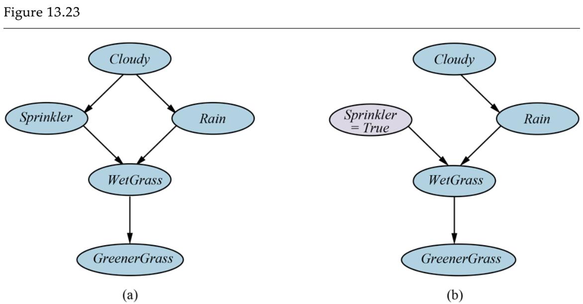
1. A causal Bayesian network representing cause–effect relations among five variables. (b) The network after performing the action “turn Sprinkler on.”

13.5.1 Representing actions: The do-operator

Consider again the Sprinkler story of Figure 13.23(a) . According to the standard semantics of Bayes nets, the joint distribution of the five variables is given by a product of five conditional distributions:

(13.14)

\[P(c, r, s, w, g) = P(c)\ P(r|c)\ P(s|c)\ P(w|r, s)\ P(g|w)\]

where we have abbreviated each variable name by its first letter. As a system of structural equations, the model looks like this:

(13.15)

\[\begin{aligned} C &=& f\_C(U\_C) \\ R &=& f\_R(C, U\_R) \\ S &=& f\_S(C, U\_S) \\ W &=& f\_W(R, S, U\_W) \\ G &=& f\_G(W, U\_G) \end{aligned}\]

where, without loss of generality, can be the identity function. The -variables in these equations represent unmodeled variables, also called error terms or disturbances, that perturb the functional relationship between each variable and its parents. For example, may represent another potential source of wetness, in addition to Sprinkler and Rain perhaps MorningDew or FirefightingHelicopter.

Unmodeled variable

If all the -variables are mutually independent random variables with suitably chosen priors, the joint distribution in Equation (13.14) can be represented exactly by the structural equations in Equation (13.16) . Thus, a system of stochastic relationships can be captured by a system of deterministic relationships, each of which is affected by an exogenous disturbance. However, the system of structural equations gives us more than that: it allows us to predict how interventions will affect the operation of the system and hence the observable consequences of those interventions. This is not possible given just the joint distribution.

For example, suppose we turn the sprinkler on—that is, if we (who are, by definition, not part of the causal processes described by the model) intervene to impose the condition . In the notation of the do-calculus, which is a key part of the theory of causal networks, this is written as . Once done, this means that the sprinkler variable is no longer dependent on whether it’s a cloudy day. We therefore delete the equation from the system of structural equations and replace it with , giving us

\[\begin{aligned} C &=& f\_C(U\_C) \\ R &=& f\_R(C, U\_R) \\ S &=&true \\ W &=& f\_W(R, S, U\_W) \\ G &=& f\_G(W, U\_G). \end{aligned}\]

Do-calculus

From these equations, we obtain the new joint distribution for the remaining variables conditioned on :

(13.17)

\[P(c, r, w, g | do (S = true) = P(c) \; P(r | c) \; P(w | r, s = true) \; P(g | w)\]

This corresponds to the “mutilated” network in Figure 13.23(b) . From Equation (13.17) , we see that the only variables whose probabilities change are WetGrass and GreenerGrass, that is, the descendants of the manipulated variable Sprinkler.

Note the difference between conditioning on the action in the original network and conditioning on the observation . The original network tells us that the sprinkler is less likely to be on when the weather is cloudy, so if we observe the sprinkler to be on, that reduces the probability that the weather is cloudy. But common sense tells us that if we (operating from outside the world, so to speak) reach in and turn on the sprinkler, that doesn’t affect the weather or provide new information about what the weather is like that day. As shown in Figure 13.23(b) , intervening breaks the normal causal link between the weather and the sprinkler. This prevents any influence flowing backward from Sprinkler to Cloudy. Thus, conditioning on in the original graph is equivalent to conditioning on in the mutilated graph.

A similar approach can be taken to analyze the effect of in a general causal network with variables . The network corresponds to a joint distribution defined in the usual way (see Equation (13.2) ):

(13.18)

\[P(x\_1, \ldots, x\_n) = \prod\_{i=1}^n P(x\_i |parent(X\_i)).\]

After applying , the new joint distribution simply omits the factor for :

(13.19)

\[P\_{x\_{jk}}(x\_1, \ldots, x\_n) \ = \left\{ \prod\_{i \neq j} P(x\_i |parents(X\_i)) = \frac{P(x\_1, \ldots, x\_n)}{P(x\_j | parents(X\_j))} \quad \text{if } \ x\_j = x\_{jk} \right\}\]

This follows from the fact that setting to a particular value corresponds to deleting the equation from the system of structural equations and replacing it with . With a bit more algebraic manipulation, one can derive a formula for the effect of setting variable on any other variable :

(13.20)

\[\begin{aligned} P(X\_i = x\_i | do(X\_j = x\_{jk}) &= & P\_{x\_{jk}}(X\_i = x\_i) \\ &= & \sum\_{p \text{vert}(X\_j)} P(x\_i | x\_{jk}, p areents(X\_j)) P(p areents(X\_j)) .\end{aligned}\]

The probability terms in the sum are obtained by computation on the original network, by any of the standard inference algorithms. This equation is known as an adjustment formula; it is a probability-weighted average of the influence of and its parents on , where the weights are the priors on the parent values. The effects of intervening on multiple variables can be computed by imagining that the individual interventions happen in sequence, each one in turn deleting the causal influences on a variable and yielding a new, mutilated model.

Adjustment formula

13.5.2 The back-door criterion

The ability to predict the effect of any intervention is a remarkable result, but it does require accurate knowledge of the necessary conditional distributions in the model, particularly . In many real-world settings, however, this is too much to ask. For example, we know that “genetic factors” play a role in obesity, but we do not know which genes play a role or the precise nature of their effects. Even in the simple story of Mary’s sprinkler decisions (Figure 13.15 , which also applies in Figure 13.23(a) ), we might know that she checks the weather before deciding whether to turn on the sprinkler, but we might not know how she makes her decision.

The specific reason this is problematic in this instance is that we would like to predict the effect of turning on the sprinkler on a downstream variable such as GreenerGrass, but the adjustment formula (Equation (13.20) ) must take into account not only the direct route from Sprinkler, but also the “back door” route via Cloudy and Rain. If we knew the value of Rain, this back-door path would be blocked—which suggests that there might be a way to write an adjustment formula that conditions on Rain instead of Cloudy. And indeed this is possible:

(13.21)

\[P(g|do | S = true) = \sum\_{r} P(g|S = true, r)P(r)\]

In general, if we wish to find the effect of on a variable , the back-door criterion allows to write an adjustment formula that conditions on any set of variables that closes the back door, so to speak. In more technical language, we want a set such that is conditionally independent of given and . This is a straightforward application of d-separation (see page 419).

Back-door criterion

The back-door criterion is a basic building block for a theory of causal reasoning that has emerged in the past two decades. It provides a way to argue against a century of statistical dogma asserting that only a randomized controlled trial can provide causal information.

The theory has provided conceptual tools and algorithms for causal analysis in a wide range of non-experimental and quasi-experimental settings; for computing probabilities on counterfactual statements (“if this had happened instead, what would the probability have been?”); for determining when findings in one population can be transferred to another; and for handling all forms of missing data when learning probability models.

Randomized controlled trial

Summary

This chapter has described Bayesian networks, a well-developed representation for uncertain knowledge. Bayesian networks play a role roughly analogous to that of propositional logic for definite knowledge.

• A Bayesian network is a directed acyclic graph whose nodes correspond to random variables; each node has a conditional distribution for the node, given its parents.
• Bayesian networks provide a concise way to represent conditional independence relationships in the domain.
• A Bayesian network specifies a joint probability distribution over its variables. The probability of any given assignment to all the variables is defined as the product of the corresponding entries in the local conditional distributions. A Bayesian network is often exponentially smaller than an explicitly enumerated joint distribution.
• Many conditional distributions can be represented compactly by canonical families of distributions. Hybrid Bayesian networks, which include both discrete and continuous variables, use a variety of canonical distributions.
• Inference in Bayesian networks means computing the probability distribution of a set of query variables, given a set of evidence variables. Exact inference algorithms, such as variable elimination, evaluate sums of products of conditional probabilities as efficiently as possible.
• In polytrees (singly connected networks), exact inference takes time linear in the size of the network. In the general case, the problem is intractable.
• Random sampling techniques such as likelihood weighting and Markov chain Monte Carlo can give reasonable estimates of the true posterior probabilities in a network and can cope with much larger networks than can exact algorithms.
• Whereas Bayes nets capture probabilistic influences, causal networks capture causal relationships and allow prediction of the effects of interventions as well as observations.

Bibliographical and Historical Notes

The use of networks to represent probabilistic information began early in the 20th century, with the work of Sewall Wright on the probabilistic analysis of genetic inheritance and animal growth factors (Wright, 1921, 1934). I. J. Good (1961), in collaboration with Alan Turing, developed probabilistic representations and Bayesian inference methods that could be regarded as a forerunner of modern Bayesian networks—although the paper is not often cited in this context. The same paper is the original source for the noisy-OR model. 7

7 I. J. Good was chief statistician for Turing’s code-breaking team in World War II. In 2001: A Space Odyssey (Clarke, 1968), Good and Minsky are credited with making the breakthrough that led to the development of the HAL 9000 computer.

The influence diagram representation for decision problems, which incorporated a DAG representation for random variables, was used in decision analysis in the late 1970s (see Chapter 16 ), but only enumeration was used for evaluation. Judea Pearl developed the message-passing method for inference in tree networks (Pearl, 1982a) and polytree networks (Kim and Pearl, 1983) and explained the importance of causal rather than diagnostic probability models. The first expert system using Bayesian networks was CONVINCE (Kim, 1983).

As chronicled in Chapter 1 , the mid-1980s saw a boom in rule-based expert systems, which incorporated ad hoc methods for handling uncertainty. Probability was considered both impractical and “cognitively implausible” as a basis for reasoning. Peter Cheeseman’s (1985) pugnacious “In Defense of Probability” and his later article “An Inquiry into Computer Understanding” (Cheeseman, 1988, with commentaries) helped to turn the tables.

The resurgence of probability depended mainly, however, on Pearl’s development of Bayesian networks and the broad development of a probabilistic approach to AI as outlined in his book, Probabilistic Reasoning in Intelligent Systems (Pearl, 1988). The book covered both representational issues, including conditional independence relationships and the dseparation criterion, and algorithmic approaches. Geiger et al. (1990a) and Tian et al. (1998) presented key computational results on efficient detection of d-separation.

Eugene Charniak helped present Pearl’s ideas to AI researchers with a popular article, “Bayesian networks without tears” (1991), and book (1993). The book by Dean and Wellman (1991) also helped introduce Bayesian networks to AI researchers. Shachter (1998) presented a simplified way to determine d-separation called the “Bayes-ball” algorithm. 8

8 The title of the original version of the article was “Pearl for swine.”

As applications of Bayes nets were developed, researchers found it necessary to go beyond the basic model of discrete variables with CPTs. For example, the CPCS system (Pradhan et al., 1994), a Bayesian network for internal medicine with 448 nodes and 906 links, made extensive use of the noisy logical operators proposed by Good (1961). Boutilier et al. (1996) analyzed the algorithmic benefits of context-specific independence. The inclusion of continuous random variables in Bayesian networks was considered by Pearl (1988) and Shachter and Kenley (1989); these papers discussed networks containing only continuous variables with linear Gaussian distributions.

Hybrid networks with both discrete and continuous variables were investigated by Lauritzen and Wermuth (1989) and implemented in the cHUGIN system (Olesen, 1993). Further analysis of linear–Gaussian models, with connections to many other models used in statistics, appears in Roweis and Ghahramani (1999); Lerner (2002) provides a very thorough discussion of their use in hybrid Bayes nets. The probit distribution is usually attributed to Gaddum (1933) and Bliss (1934), although it had been discovered several times in the 19th century. Bliss’s work was expanded considerably by Finney (1947). The probit has been used widely for modeling discrete choice phenomena and can be extended to handle more than two choices (Daganzo, 1979). The expit (inverse logit) model was introduced by Berkson (1944); initially much derided, it eventually became more popular than the probit model. Bishop (1995) gives a simple justification for its use.

Early applications of Bayes nets in medicine included the MUNIN system for diagnosing neuromuscular disorders (Andersen et al., 1989) and the PATHFINDER system for pathology (Heckerman, 1991). Applications in engineering include the Electric Power Research Institute’s work on monitoring power generators (Morjaria et al., 1995), NASA’s work on displaying time-critical information at Mission Control in Houston (Horvitz and Barry, 1995), and the general field of network tomography, which aims to infer unobserved local properties of nodes and links in the Internet from observations of end-to-end message performance (Castro et al., 2004). Perhaps the most widely used Bayesian network systems have been the diagnosis-and-repair modules (e.g., the Printer Wizard) in Microsoft Windows (Breese and Heckerman, 1996) and the Office Assistant in Microsoft Office (Horvitz et al., 1998).

Another important application area is biology: the mathematical models used to analyze genetic inheritance in family trees (so-called pedigree analysis) are in fact a special form of Bayesian networks. Exact inference algorithms for pedigree analysis, resembling variable elimination, were developed in the 1970s (Cannings et al., 1978). Bayesian networks have been used for identifying human genes by reference to mouse genes (Zhang et al., 2003), inferring cellular networks (Friedman, 2004), genetic linkage analysis to locate diseaserelated genes (Silberstein et al., 2013), and many other tasks in bioinformatics. We could go on, but instead we’ll refer you to Pourret et al. (2008), a 400-page guide to applications of Bayesian networks. Published applications over the last decade run into the tens of thousands, ranging from dentistry to global climate models.

Pedigree analysis

Judea Pearl (1985), in the first paper to use the term “Bayesian networks,” briefly described an inference algorithm for general networks based on the cutset conditioning idea introduced in Chapter 6 . Independently, Ross Shachter (1986), working in the influence diagram community, developed a complete algorithm based on goal-directed reduction of the network using posterior-preserving transformations.

Pearl (1986) developed a clustering algorithm for exact inference in general Bayesian networks, utilizing a conversion to a directed polytree of clusters in which message passing was used to achieve consistency over variables shared between clusters. A similar approach, developed by the statisticians David Spiegelhalter and Steffen Lauritzen (Lauritzen and Spiegelhalter, 1988), is based on conversion to an undirected form of graphical model called a Markov network. This approach is implemented in the HUGIN system, an efficient and widely used tool for uncertain reasoning (Andersen et al., 1989).

The basic idea of variable elimination—that repeated computations within the overall sumof-products expression can be avoided by caching—appeared in the symbolic probabilistic inference (SPI) algorithm (Shachter et al., 1990). The elimination algorithm we describe is closest to that developed by Zhang and Poole (1994). Criteria for pruning irrelevant variables were developed by Geiger et al. (1990b) and by Lauritzen et al. (1990); the criterion we give is a simple special case of these. Dechter (1999) shows how the variable elimination idea is essentially identical to nonserial dynamic programming (Bertele and Brioschi, 1972).

Nonserial dynamic programming

This connects Bayesian network algorithms to related methods for solving CSPs and gives a direct measure of the complexity of exact inference in terms of the tree width of the network. Preventing the exponential growth in the size of factors in variable elimination can be done by dropping variables from large factors (Dechter and Rish, 2003); it also also possible to bound the error introduced thereby (Wexler and Meek, 2009). Alternatively, factors can be compressed by representing them using algebraic decision diagrams instead of tables (Gogate and Domingos, 2011).

Exact methods based on recursive enumeration (see Figure 13.11 ) combined with caching include the recursive conditioning algorithm (Darwiche, 2001), the value elimination algorithm (Bacchus et al., 2003), and AND–OR search (Dechter and Mateescu, 2007). The method of weighted model counting (Sang et al., 2005; Chavira and Darwiche, 2008) is usually based on a DPLL-style SAT solver (see Figure 7.17 on page 234). As such, it is also performing a recursive enumeration of variable assignments with caching, so the approach is in fact quite similar. All three of these algorithms can implement a complete range of space/time tradeoffs. Because they consider variable assignments, the algorithms can easily take advantage of determinism and context-specific independence in the model. They can also be modified to use an efficient linear-time algorithm whenever the partial assignment makes the remaining network a polytree. (This is a version of the method of cutset conditioning, which was described for CSPs in Chapter 6 .) For exact inference in large

models, where the space requirements of clustering and variable elimination become enormous, these recursive algorithms are often the most practical approach.

There are other important inference tasks in Bayes nets besides computing marginal probabilities. The most probable explanation or MPE is the most likely assignment to the nonevidence variables given the evidence. (MPE is a special case of MAP—maximum a posteriori—inference, which asks for the most likely assignment to a subset of nonevidence variables given the evidence.) For such problems, many different algorithms have been developed, some related to shortest-path or AND–OR search algorithms; for a summary, see Marinescu and Dechter (2009).

Most probable explanation

The first result on the complexity of inference in Bayes nets is due to Cooper (1990), who showed that the general problem of computing marginals in Bayesian networks is NP-hard; as noted in the chapter, this can be strengthened to #P-hardness through a reduction from counting satisfying assignments (Roth, 1996). This also implies the NP-hardness of approximate inference (Dagum and Luby, 1993); however, for the case where probabilities can be bounded away from 0 and 1, a form of likelihood weighting converges in (randomized) polynomial time (Dagum and Luby, 1997). Shimony (1994) showed that finding the most probable explanation is NP-complete—intractable, but somewhat easier than computing marginals—while Park and Darwiche (2004) provide a thorough complexity analysis of MAP computation, showing that it falls into the class of -complete problems —that is, somewhat harder than computing marginals.

The development of fast approximation algorithms for Bayesian network inference is a very active area, with contributions from statistics, computer science, and physics. The rejection sampling method is a general technique dating back at least to Buffon’s needle (1777); it was first applied to Bayesian networks by Max Henrion (1988), who called it logic sampling. Importance sampling was invented originally for applications in physics (Kahn, 1950a, 1950b) and applied to Bayes net inference by Fung and Chang (1989) (who called the algorithm “evidence weighting”) and by Shachter and Peot (1989).

In statistics, adaptive sampling has been applied to all sorts of Monte Carlo algorithms to speed up convergence. The basic idea is to adapt the distribution from which samples are generated, based on the outcome from previous samples. Gilks and Wild (1992) developed adaptive rejection sampling, while adaptive importance sampling appears to have originated independently in physics (Lepage, 1978), civil engineering (Karamchandani et al., 1989), statistics (Oh and Berger, 1992), and computer graphics (Veach and Guibas, 1995). Cheng and Druzdzel (2000) describe an adaptive version of importance sampling applied to Bayes net inference. More recently, Le et al. (2017) have demonstrated the use of deep learning systems to produce proposal distributions that speed up importance sampling by many orders of magnitude.

Markov chain Monte Carlo (MCMC) algorithms began with the Metropolis algorithm, due to Metropolis et al. (1953), which was also the source of the simulated annealing algorithm described in Chapter 4 . Hastings (1970) introduced the accept/reject step that is an integral part of what we now call the Metropolis–Hastings algorithm. The Gibbs sampler was devised by Geman and Geman (1984) for inference in undirected Markov networks. The application of Gibbs sampling to Bayesian networks is due to Pearl (1987). The papers collected by Gilks et al. (1996) cover both theory and applications of MCMC.

Since the mid-1990s, MCMC has become the workhorse of Bayesian statistics and statistical computation in many other disciplines including physics and biology. The Handbook of Markov Chain Monte Carlo (Brooks et al., 2011) covers many aspects of this literature. The BUGS package (Gilks et al., 1994) was an early and influential system for Bayes net modeling and inference using Gibbs sampling. STAN (named after Stanislaw Ulam, an originator of Monte Carlo methods in physics) is a more recent system that uses Hamiltonian Monte Carlo inference (Carpenter et al., 2017).

There are two very important families of approximation methods that we did not cover in the chapter. The first is the family of variational approximation methods, which can be used to simplify complex calculations of all kinds. The basic idea is to propose a reduced version of the original problem that is simple to work with, but that resembles the original problem as closely as possible. The reduced problem is described by some variational parameters that are adjusted to minimize a distance function between the original and the reduced problem, often by solving the system of equations . In many cases, strict upper and lower bounds can be obtained. Variational methods have long been used in statistics (Rustagi, 1976). In statistical physics, the mean-field method is a particular variational approximation in which the individual variables making up the model are assumed to be completely independent.

This idea was applied to solve large undirected Markov networks (Peterson and Anderson, 1987; Parisi, 1988). Saul et al. (1996) developed the mathematical foundations for applying variational methods to Bayesian networks and obtained accurate lower-bound approximations for sigmoid networks with the use of mean-field methods. Jaakkola and Jordan (1996) extended the methodology to obtain both lower and upper bounds. Since these early papers, variational methods have been applied to many specific families of models. The remarkable paper by Wainwright and Jordan (2008) provides a unifying theoretical analysis of the literature on variational methods.

A second important family of approximation algorithms is based on Pearl’s polytree message-passing algorithm (1982a). This algorithm can be applied to general “loopy” networks, as suggested by Pearl (1988). The results might be incorrect, or the algorithm might fail to terminate, but in many cases, the values obtained are close to the true values. Little attention was paid to this so-called loopy belief propagation approach until McEliece et al. (1998) observed that it is exactly the computation performed by the turbo decoding algorithm (Berrou et al., 1993), which provided a major breakthrough in the design of efficient error-correcting codes.

Loopy belief propagation

Turbo decoding

The implication of these observations is if loopy BP is both fast and accurate on the very large and very highly connected networks used for decoding, it might therefore be useful more generally. Theoretical support for these findings, including convergence proofs for

some special cases, was provided by Weiss (2000b), Weiss and Freeman (2001), Yedidia et al. (2005), drawing on connections to ideas from statistical physics.

Theories of causal inference going beyond randomized controlled trials were proposed by Rubin (1974) and Robins (1986), but these ideas remained both obscure and controversial until Judea Pearl developed and presented a fully articulated theory of causality based on causal networks (Pearl, 2000). Peters et al. (2017) further develop the theory, with an emphasis on learning. A more recent work, The Book of Why (Pearl and McKenzie, 2018), provides a less mathematical but more readable and wide-ranging introduction.

Uncertain reasoning in AI has not always been based on probability theory. As noted in Chapter 12 , early probabilistic systems fell out of favor in the early 1970s, leaving a partial vacuum to be filled by alternative methods. These included rule-based expert systems, Dempster–Shafer theory, and (to some extent) fuzzy logic. 9

9 A fourth approach, default reasoning, treats conclusions not as “believed to a certain degree,” but as “believed until a better reason is found to believe something else.” It is covered in Chapter 10 .

Rule-based approaches to uncertainty hoped to build on the success of logical rule-based systems, but add a sort of “fudge factor”—more politely called a certainty factor—to each rule to accommodate uncertainty. The first such system was MYCIN (Shortliffe, 1976), a medical expert system for bacterial infections. The collection Rule-Based Expert Systems (Buchanan and Shortliffe, 1984) provides a complete overview of MYCIN and its descendants (see also Stefik, 1995).

David Heckerman (1986) showed that a slightly modified version of certainty factor calculations gives correct probabilistic results in some cases, but results in serious overcounting of evidence in other cases. As rule sets became larger, undesirable interactions between rules became more common, and practitioners found that the certainty factors of many other rules had to be “tweaked” when new rules were added. The basic mathematical properties that allow chains of reasoning in logic simply do not hold for probability.

Dempster–Shafer theory originates with a paper by Arthur Dempster (1968) proposing a generalization of probability to interval values and a combination rule for using them. Such an approach might alleviate the difficulty of specifying probabilities exactly. Later work by Glenn Shafer (1976) led to the Dempster–Shafer theory’s being viewed as a competing

approach to probability. Pearl (1988) and Ruspini et al. (1992) analyze the relationship between the Dempster–Shafer theory and standard probability theory. In many cases, probability theory does not require probabilities to be specified exactly: we can express uncertainty about probability values as (second-order) probability distributions, as explained in Chapter 20 .

Fuzzy sets were developed by Lotfi Zadeh (1965) in response to the perceived difficulty of providing exact inputs to intelligent systems. A fuzzy set is one in which membership is a matter of degree. Fuzzy logic is a method for reasoning with logical expressions describing membership in fuzzy sets. Fuzzy control is a methodology for constructing control systems in which the mapping between real-valued input and output parameters is represented by fuzzy rules. Fuzzy control has been very successful in commercial products such as automatic transmissions, video cameras, and electric shavers. The text by Zimmermann (2001) provides a thorough introduction to fuzzy set theory; papers on fuzzy applications are collected in Zimmermann (1999).

Fuzzy logic has often been perceived incorrectly as a direct competitor to probability theory, whereas in fact it addresses a different set of issues: rather than considering uncertainty about the truth of well-defined propositions, fuzzy logic handles vagueness in the mapping from terms in a symbolic theory to an actual world. Vagueness is a real issue in any application of logic, probability, or indeed standard mathematical models to reality. Even a variable as impeccable as the mass of the Earth turns out, on inspection, to vary with time as meteorites and molecules come and go. It is also imprecise—does it include the atmosphere? If so, to what height? In some cases, further elaboration of the model can reduce vagueness, but fuzzy logic takes vagueness as a given and develops a theory around it.

Possibility theory (Zadeh, 1978) was introduced to handle uncertainty in fuzzy systems and has much in common with probability (Dubois and Prade, 1994).

Many AI researchers in the 1970s rejected probability because the numerical calculations that probability theory was thought to require were not apparent to introspection and presumed an unrealistic level of precision in our uncertain knowledge. The development of qualitative probabilistic networks (Wellman, 1990a) provided a purely qualitative abstraction of Bayesian networks, using the notion of positive and negative influences between variables. Wellman shows that in many cases such information is sufficient for

optimal decision making without the need for the precise specification of probability values. Goldszmidt and Pearl (1996) take a similar approach. Work by Darwiche and Ginsberg (1992) extracts the basic properties of conditioning and evidence combination from probability theory and shows that they can also be applied in logical and default reasoning.

Several excellent texts (Jensen, 2007; Darwiche, 2009; Koller and Friedman, 2009; Korb and Nicholson, 2010; Dechter, 2019) provide thorough treatments of the topics we have covered in this chapter. New research on probabilistic reasoning appears both in mainstream AI journals, such as Artificial Intelligence and the Journal of AI Research, and in more specialized journals, such as the International Journal of Approximate Reasoning. Many papers on graphical models, which include Bayesian networks, appear in statistical journals. The proceedings of the conferences on Uncertainty in Artificial Intelligence (UAI), Neural Information Processing Systems (NeurIPS), and Artificial Intelligence and Statistics (AISTATS) are good sources for current research.

Chapter 14 Probabilistic Reasoning over Time

In which we try to interpret the present, understand the past, and perhaps predict the future, even when very little is crystal clear.

Agents in partially observable environments must be able to keep track of the current state, to the extent that their sensors allow. In Section 4.4 we showed a methodology for doing that: an agent maintains a belief state that represents which states of the world are currently possible. From the belief state and a transition model, the agent can predict how the world might evolve in the next time step. From the percepts observed and a sensor model, the agent can update the belief state. This is a pervasive idea: in Chapter 4 belief states were represented by explicitly enumerated sets of states, whereas in Chapters 7 and 11 they were represented by logical formulas. Those approaches defined belief states in terms of which world states were possible, but could say nothing about which states were likely or unlikely. In this chapter, we use probability theory to quantify the degree of belief in elements of the belief state.

As we show in Section 14.1 , time itself is handled in the same way as in Chapter 7 : a changing world is modeled using a variable for each aspect of the world state at each point in time. The transition and sensor models may be uncertain: the transition model describes the probability distribution of the variables at time , given the state of the world at past times, while the sensor model describes the probability of each percept at time , given the current state of the world. Section 14.2 defines the basic inference tasks and describes the general structure of inference algorithms for temporal models. Then we describe three specific kinds of models: hidden Markov models, Kalman filters, and dynamic Bayesian networks (which include hidden Markov models and Kalman filters as special cases).

14.1 Time and Uncertainty

We have developed our techniques for probabilistic reasoning in the context of static worlds, in which each random variable has a single fixed value. For example, when repairing a car, we assume that whatever is broken remains broken during the process of diagnosis; our job is to infer the state of the car from observed evidence, which also remains fixed.

Now consider a slightly different problem: treating a diabetic patient. As in the case of car repair, we have evidence such as recent insulin doses, food intake, blood sugar measurements, and other physical signs. The task is to assess the current state of the patient, including the actual blood sugar level and insulin level. Given this information, we can make a decision about the patient’s food intake and insulin dose. Unlike the case of car repair, here the dynamic aspects of the problem are essential. Blood sugar levels and measurements thereof can change rapidly over time, depending on recent food intake and insulin doses, metabolic activity, the time of day, and so on. To assess the current state from the history of evidence and to predict the outcomes of treatment actions, we must model these changes.

The same considerations arise in many other contexts, such as tracking the location of a robot, tracking the economic activity of a nation, and making sense of a spoken or written sequence of words. How can dynamic situations like these be modeled?

14.1.1 States and observations

This chapter discusses discrete-time models, in which the world is viewed as a series of snapshots or time slices. We’ll just number the time slices 0, 1, 2, and so on, rather than assigning specific times to them. Typically, the time interval between slices is assumed to be the same for every interval. For any particular application, a specific value of has to be chosen. Sometimes this is dictated by the sensor; for example, a video camera might supply images at intervals of of a second. In other cases, the interval is dictated by the typical rates of change of the relevant variables; for example, in the case of blood glucose monitoring, things can change significantly in the course of ten minutes, so a one-minute 1

interval might be appropriate. On the other hand, in modeling continental drift over geological time, an interval of a million years might be fine.

1 Uncertainty over continuous time can be modeled by stochastic differential equations (SDEs). The models studied in this chapter can be viewed as discrete-time approximations to SDEs.

Discrete time

Time slice

Each time slice in a discrete-time probability model contains a set of random variables, some observable and some not. For simplicity, we will assume that the same subset of variables is observable in each time slice (although this is not strictly necessary in anything that follows). We will use to denote the set of state variables at time , which are assumed to be unobservable, and to denote the set of observable evidence variables. The observation at time is for some set of values .

Consider the following example: You are the security guard stationed at a secret underground installation. You want to know whether it’s raining today, but your only access to the outside world occurs each morning when you see the director coming in with, or without, an umbrella. For each day , the set thus contains a single evidence variable or for short (whether the umbrella appears), and the set contains a single state variable or for short (whether it is raining). Other problems can involve larger sets of variables. In the diabetes example, the evidence variables might be and while the state variables might include and . (Notice that and are not the same variable; this is how we deal with noisy measurements of actual quantities.)

We will assume that the state sequence starts at and evidence starts arriving at . Hence, our umbrella world is represented by state variables and evidence variables . We will use the notation to denote the sequence of integers from to inclusive and the notation to denote the set of variables from to inclusive. For example, corresponds to , , . (Note that this is different from the notation used in programming languages such as Python and Go, where U[1:3] would not include U[3].)

14.1.2 Transition and sensor models

With the set of state and evidence variables for a given problem decided on, the next step is to specify how the world evolves (the transition model) and how the evidence variables get their values (the sensor model).

The transition model specifies the probability distribution over the latest state variables, given the previous values, that is, . Now we face a problem: the set is unbounded in size as increases. We solve the problem by making a Markov assumption that the current state depends on only a finite fixed number of previous states. Processes satisfying this assumption were first studied in depth by the statistician Andrei Markov (1856–1922) and are called Markov processes or Markov chains. They come in various flavors; the simplest is the first-order Markov process, in which the current state depends only on the previous state and not on any earlier states. In other words, a state provides enough information to make the future conditionally independent of the past, and we have

(14.1)

\[\mathbf{P}(\mathbf{X}\_t|\mathbf{X}\_{0:t-1}) = \mathbf{P}(\mathbf{X}\_t|\mathbf{X}\_{t-1}).\]

Markov assumption

Markov process

First-order Markov process

Hence, in a first-order Markov process, the transition model is the conditional distribution . The transition model for a second-order Markov process is the conditional distribution . Figure 14.1 shows the Bayesian network structures corresponding to first-order and second-order Markov processes.

Figure 14.1

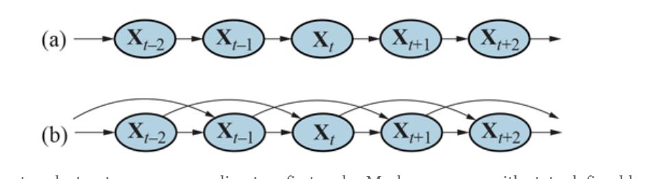
1. Bayesian network structure corresponding to a first-order Markov process with state defined by the variables . (b) A second-order Markov process.

Even with the Markov assumption there is still a problem: there are infinitely many possible values of . Do we need to specify a different distribution for each time step? We avoid this problem by assuming that changes in the world state are caused by a time-homogeneous process—that is, a process of change that is governed by laws that do not themselves change over time. In the umbrella world, then, the conditional probability of rain, , is the same for all , and we need specify only one conditional probability table.

Time-homogeneous

Now for the sensor model. The evidence variables could depend on previous variables as well as the current state variables, but any state that’s worth its salt should suffice to generate the current sensor values. Thus, we make a sensor Markov assumption as follows:

(14.2)

\[\mathbf{P}(\mathbf{E}\_t|\mathbf{X}\_{0:t}, \mathbf{E}\_{1:t-1}) = \mathbf{P}(\mathbf{E}\_t|\mathbf{X}\_t).\]

Thus, is our sensor model (sometimes called the observation model). Figure 14.2 shows both the transition model and the sensor model for the umbrella example. Notice the direction of the dependence between state and sensors: the arrows go from the actual state of the world to sensor values because the state of the world causes the sensors to take on particular values: the rain causes the umbrella to appear. (The inference process, of course, goes in the other direction; the distinction between the direction of modeled dependencies and the direction of inference is one of the principal advantages of Bayesian networks.)

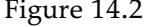
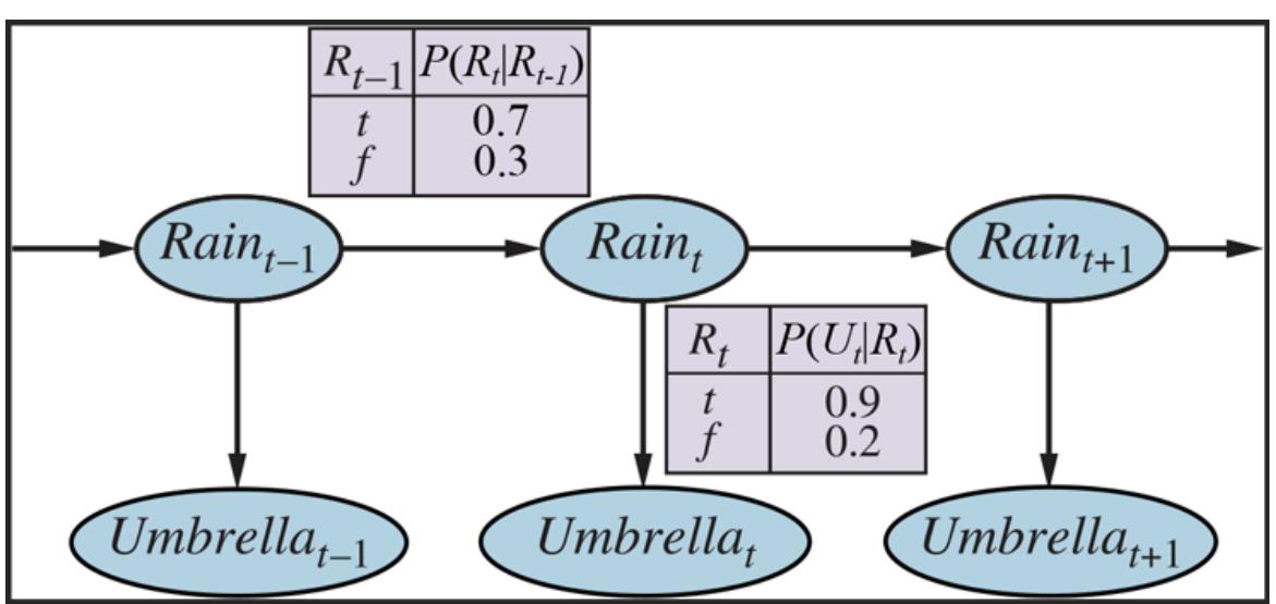
Bayesian network structure and conditional distributions describing the umbrella world. The transition model is and the sensor model is .

In addition to specifying the transition and sensor models, we need to say how everything gets started—the prior probability distribution at time 0, . With that, we have a specification of the complete joint distribution over all the variables, using Equation (13.2) . For any time step ,

(14.3)

\[\mathbf{P}(\mathbf{X}\_{0:t}, \mathbf{E}\_{1:t}) = \mathbf{P}(\mathbf{X}\_0) \prod\_{i=1}^{t} \mathbf{P}(\mathbf{X}\_i | \mathbf{X}\_{i-1}) \mathbf{P}(\mathbf{E}\_i | \mathbf{X}\_i).\]

The three terms on the right-hand side are the initial state model , the transition model , and the sensor model . This equation defines the semantics of the family of temporal models represented by the three terms. Notice that standard Bayesian networks cannot represent such models because they require a finite set of variables. The ability to handle an infinite set of variables comes from two things: first, defining the infinite set using integer indices; and second, the use of implicit universal quantification (see Section 8.2 ) to define the sensor and transition models for every time step.

The structure in Figure 14.2 is a first-order Markov process—the probability of rain is assumed to depend only on whether it rained the previous day. Whether such an assumption is reasonable depends on the domain itself. The first-order Markov assumption says that the state variables contain all the information needed to characterize the probability distribution for the next time slice. Sometimes the assumption is exactly true for example, if a particle is executing a random walk along the -axis, changing its position by at each time step, then using the -coordinate as the state gives a first-order Markov process. Sometimes the assumption is only approximate, as in the case of predicting rain only on the basis of whether it rained the previous day. There are two ways to improve the accuracy of the approximation:

• 1. Increasing the order of the Markov process model. For example, we could make a second-order model by adding as a parent of , which might give slightly more accurate predictions. For example, in Palo Alto, California, it very rarely rains more than two days in a row.
• 2. Increasing the set of state variables. For example, we could add to allow us to incorporate historical records of rainy seasons, or we could add , , and (perhaps at a range of locations) to allow us to use a physical model of rainy conditions.

Exercise 14.AUGM asks you to show that the first solution—increasing the order—can always be reformulated as an increase in the set of state variables, keeping the order fixed. Notice that adding state variables might improve the system’s predictive power but also increases the prediction requirements: we now have to predict the new variables as well. Thus, we are looking for a “self-sufficient” set of variables, which really means that we have to understand the “physics” of the process being modeled. The requirement for accurate modeling of the

process is obviously lessened if we can add new sensors (e.g., measurements of temperature and pressure) that provide information directly about the new state variables.

Consider, for example, the problem of tracking a robot wandering randomly on the plane. One might propose that the position and velocity are a sufficient set of state variables: one can simply use Newton’s laws to calculate the new position, and the velocity may change unpredictably. If the robot is battery-powered, however, then battery exhaustion would tend to have a systematic effect on the change in velocity. Because this in turn depends on how much power was used by all previous maneuvers, the Markov property is violated.

We can restore the Markov property by including the charge level as one of the state variables that make up . This helps in predicting the motion of the robot, but in turn requires a model for predicting from and the velocity. In some cases, that can be done reliably, but more often we find that error accumulates over time. In that case, accuracy can be improved by adding a new sensor for the battery level. We will return to the battery example in Section 14.5 .

14.2 Inference in Temporal Models

Having set up the structure of a generic temporal model, we can formulate the basic inference tasks that must be solved:

Filtering or state estimation is the task of computing the belief state —the posterior distribution over the most recent state given all evidence to date. In the umbrella example, this would mean computing the probability of rain today, given all the umbrella observations made so far. Filtering is what a rational agent does to keep track of the current state so that rational decisions can be made. It turns out that an almost identical calculation provides the likelihood of the evidence sequence, . 2 The term “filtering” refers to the roots of this problem in early work on signal processing, where the problem is to filter out the noise in a signal by estimating its underlying properties. 2

Filtering

State estimation

Belief state

PREDICTION: This is the task of computing the posterior distribution over the future state, given all evidence to date. That is, we wish to compute for some . In the umbrella example, this might mean computing the probability of rain three days from now, given all the observations to date. Prediction is useful for evaluating possible courses of action based on their expected outcomes.

Prediction

Smoothing

SMOOTHING: This is the task of computing the posterior distribution over a past state, given all evidence up to the present. That is, we wish to compute for some such that . In the umbrella example, it might mean computing the probability that it rained last Wednesday, given all the observations of the umbrella carrier made up to today. Smoothing provides a better estimate of the state at time than was available at that time, because it incorporates more evidence. 3

3 In particular, when tracking a moving object with inaccurate position observations, smoothing gives a smoother estimated trajectory than filtering—hence the name.

MOST LIKELY EXPLANATION: Given a sequence of observations, we might wish to find the sequence of states that is most likely to have generated those observations. That is, we wish to compute . For example, if the umbrella appears on each of the first three days and is absent on the fourth, then the most likely explanation is that it rained on the first three days and did not rain on the fourth. Algorithms for this task are useful in many applications, including speech recognition—where the aim is to find the most likely sequence of words, given a series of sounds—and the reconstruction of bit strings transmitted over a noisy channel.

In addition to these inference tasks, we also have

LEARNING: The transition and sensor models, if not yet known, can be learned from observations. Just as with static Bayesian networks, dynamic Bayes net learning can be done as a by-product of inference. Inference provides an estimate of what transitions actually occurred and of what states generated the sensor readings, and these estimates can be used to learn the models. The learning process can operate via an iterative update algorithm called expectation–maximization or EM, or it can result from Bayesian updating of the model parameters given the evidence. See Chapter 20 for more details. The remainder of this section describes generic algorithms for the four inference tasks, independent of the particular kind of model employed. Improvements specific to each model are described in subsequent sections.

14.2.1 Filtering and prediction

As we pointed out in Section 7.7.3 , a useful filtering algorithm needs to maintain a current state estimate and update it, rather than going back over the entire history of percepts for each update. (Otherwise, the cost of each update increases as time goes by.) In other words, given the result of filtering up to time , the agent needs to compute the result for from the new evidence . So we have

\[\mathbf{P}(\mathbf{X}\_{t+1}|\mathbf{e}\_{1:t+1}) = f(\mathbf{e}\_{t+1}, \mathbf{P}(\mathbf{X}\_t|\mathbf{e}\_{1:t})) \]

for some function . This process is called recursive estimation. (See also Sections 4.4 and 7.7.3 .) We can view the calculation as being composed of two parts: first, the current state distribution is projected forward from to ; then it is updated using the new evidence . This two-part process emerges quite simply when the formula is rearranged:

(14.4)

\[\begin{aligned} \mathbf{P}\left(\mathbf{X}\_{t+1}|\mathbf{e}\_{1:t+1}\right) &= \mathbf{P}\left(\mathbf{X}\_{t+1}|\mathbf{e}\_{1:t},\mathbf{e}\_{t+1}\right) \quad \text{(dividing up the evidence)}\\ &= \alpha \mathbf{P}\left(\mathbf{e}\_{t+1}|\mathbf{X}\_{t+1},\mathbf{e}\_{1:t}\right) \mathbf{P}\left(\mathbf{X}\_{t+1}|\mathbf{e}\_{1:t}\right) \quad \text{(using Bayes' rule, given } \mathbf{e}\_{1:t})\\ &= \alpha \underbrace{\mathbf{P}\left(\mathbf{e}\_{t+1}|\mathbf{X}\_{t+1}\right) \mathbf{P}\left(\mathbf{X}\_{t+1}|\mathbf{e}\_{1:t}\right)}\_{\text{update}} \quad \text{(by the sensor Markov assumption)}. \end{aligned}\]

Here and throughout this chapter, is a normalizing constant used to make probabilities sum up to 1. Now we plug in an expression for the one-step prediction , obtained by conditioning on the current state . The resulting equation for the new state estimate is the central result in this chapter:

(14.5)

\[\begin{split} \mathbf{P}\left(\mathbf{X}\_{t+1}|\mathbf{e}\_{1:t+1}\right) &= \alpha \mathbf{P}\left(\mathbf{e}\_{t+1}|\mathbf{X}\_{t+1}\right) \sum\_{\mathbf{X}\_{t}} \mathbf{P}\left(\mathbf{X}\_{t+1}|\mathbf{x}\_{t},\mathbf{e}\_{1:t}\right) P\left(\mathbf{x}\_{t}|\mathbf{e}\_{1:t}\right) \\ &= \alpha \underbrace{\mathbf{P}\left(\mathbf{e}\_{t+1}|\mathbf{X}\_{t+1}\right)}\_{\text{sensor model}} \sum\_{\mathbf{x}\_{t}} \underbrace{\mathbf{P}\left(\mathbf{X}\_{t+1}|\mathbf{x}\_{t}\right)}\_{\text{transition model}} \underbrace{P\left(\mathbf{x}\_{t}|\mathbf{e}\_{1:t}\right)}\_{\text{recursion model}} \text{ (Markov assumption)}. \end{split}\]

In this expression, all the terms come either from the model or from the previous state estimate. Hence, we have the desired recursive formulation. We can think of the filtered estimate as a “message” that is propagated forward along the sequence, modified by each transition and updated by each new observation. The process is given by

\[\mathbf{f}\_{1:t+1} = \text{ForwARD}(\mathbf{f}\_{1:t}, \mathbf{e}\_{t+1}).\]

where FORWARD implements the update described in Equation (14.5) and the process begins with . When all the state variables are discrete, the time for each update is constant (i.e., independent of ), and the space required is also constant. (The constants depend, of course, on the size of the state space and the specific type of the temporal model in question.) The time and space requirements for updating must be constant if a finite agent is to keep track of the current state distribution indefinitely.

Let us illustrate the filtering process for two steps in the basic umbrella example (Figure 14.2 ). That is, we will compute as follows:

• On day 0, we have no observations, only the security guard’s prior beliefs; let’s assume that consists of .
• On day 1, the umbrella appears, so . The prediction from to is

\[\begin{aligned} \mathbf{P}(R\_1) &= \sum\_{r\_0} \mathbf{P}(R\_1|r\_0)P(r\_0) \\ &= \langle 0.7, 0.3 \rangle \times 0.5 + \langle 0.3, 0.7 \rangle \times 0.5 = \langle 0.5, 0.5 \rangle. \end{aligned}\]

Then the update step simply multiplies by the probability of the evidence for and normalizes, as shown in Equation (14.4) :

\[\begin{aligned} \mathbf{P}(R\_1|u\_1) &= \alpha \mathbf{P}(u\_1|R\_1)\mathbf{P}(R\_1) = \alpha \left< 0.9, 0.2 \right> \left< 0.5, 0.5 \right> \\ &= \alpha \left< 0.45, 0.1 \right> \approx \left< 0.818, 0.182 \right>. \end{aligned}\]

On day 2, the umbrella appears, so . The prediction from to is

\[\begin{aligned} \mathbf{P}(R\_2|u\_1) &= \sum\_{r\_1} \mathbf{P}(R\_2|r\_1)P(r\_1|u\_1) \\ &= \langle 0.7, 0.3 \rangle \times 0.818 + \langle 0.3, 0.7 \rangle \times 0.182 \approx \langle 0.627, 0.373 \rangle \end{aligned}\]

and updating it with the evidence for gives

\[\begin{aligned} \mathbf{P}(R\_2|u\_1, u\_2) &= \alpha \mathbf{P}(u\_2|R\_2)\mathbf{P}(R\_2|u\_1) = \alpha \left< 0.9, 0.2 \right> \left< 0.627, 0.373 \right> \\ &= \alpha \left< 0.565, 0.075 \right> \approx \left< 0.883, 0.117 \right>. \end{aligned}\]

Intuitively, the probability of rain increases from day 1 to day 2 because rain persists. Exercise 14.CONV(a) asks you to investigate this tendency further.

The task of prediction can be seen simply as filtering without the addition of new evidence. In fact, the filtering process already incorporates a one-step prediction, and it is easy to derive the following recursive computation for predicting the state at from a prediction for :

(14.6)

\[\mathbf{P}(\mathbf{X}\_{t+k+1}|\mathbf{e}\_{1:t}) = \sum\_{\mathbf{x}\_{t+k}} \underbrace{\mathbf{P}(\mathbf{X}\_{t+k+1}|\mathbf{x}\_{t+k}) P(\mathbf{x}\_{t+k}|\mathbf{e}\_{1:t})}\_{\text{transition model}}.\]

Naturally, this computation involves only the transition model and not the sensor model.

It is interesting to consider what happens as we try to predict further and further into the future. As Exercise 14.CONV(b) shows, the predicted distribution for rain converges to a fixed point , after which it remains constant for all time. This is the stationary distribution of the Markov process defined by the transition model. (See also 444.) A great deal is known about the properties of such distributions and about the mixing time roughly, the time taken to reach the fixed point. In practical terms, this dooms to failure any attempt to predict the actual state for a number of steps that is more than a small fraction of the mixing time, unless the stationary distribution itself is strongly peaked in a small area of the state space. The more uncertainty there is in the transition model, the shorter will be the mixing time and the more the future is obscured. 4

4 If one picks an arbitrary day to be , then it makes sense to choose the prior to match the stationary distribution, which is why we picked as the prior. Had we picked a different prior, the stationary distribution would still have worked out to .

In addition to filtering and prediction, we can use a forward recursion to compute the likelihood of the evidence sequence, . This is a useful quantity if we want to compare different temporal models that might have produced the same evidence sequence (e.g., two different models for the persistence of rain). For this recursion, we use a likelihood message

. It is easy to show (Exercise 14.LIKL) that the message calculation is identical to that for filtering:

\[l\_{1:t+1} = \text{FORWardD}(l\_{1:t}, \mathbf{e}\_{t+1}).\]

Having computed , we obtain the actual likelihood by summing out :

(14.7)

\[L\_{1:t} = P(\mathbf{e}\_{1:t}) = \sum\_{\mathbf{x}\_t} l\_{1:t}(\mathbf{x}\_t).\]

Notice that the likelihood message represents the probabilities of longer and longer evidence sequences as time goes by and so becomes numerically smaller and smaller, leading to underflow problems with floating-point arithmetic. This is an important problem in practice, but we shall not go into solutions here.

14.2.2 Smoothing

As we said earlier, smoothing is the process of computing the distribution over past states given evidence up to the present—that is, for . (See Figure 14.3 .) In anticipation of another recursive message-passing approach, we can split the computation into two parts—the evidence up to and the evidence from to ,

(14.8)

\[\begin{split} \mathbf{P}(\mathbf{X}\_{k}|\mathbf{e}\_{1:t}) &= \mathbf{P}(\mathbf{X}\_{k}|\mathbf{e}\_{1:k}, \mathbf{e}\_{k+1:t}) \\ &= \alpha \mathbf{P}(\mathbf{X}\_{k}|\mathbf{e}\_{1:k}) \mathbf{P}(\mathbf{e}\_{k+1:t}|\mathbf{X}\_{k}, \mathbf{e}\_{1:k}) \quad \text{(using Bayes' rule, given } \mathbf{e}\_{1:k}) \\ &= \alpha \mathbf{P}(\mathbf{X}\_{k}|\mathbf{e}\_{1:k}) \mathbf{P}(\mathbf{e}\_{k+1:t}|\mathbf{X}\_{k}) \quad \text{(using conditional independence)} \\ &= \alpha \mathbf{f}\_{1:k} \times \mathbf{b}\_{k+1:t}. \end{split}\]

Figure 14.3

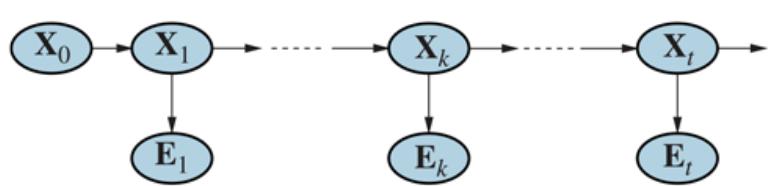
Smoothing computes , the posterior distribution of the state at some past time given a complete sequence of observations from to .

where ” ” represents pointwise multiplication of vectors. Here we have defined a “backward” message , analogous to the forward message . The forward message can be computed by filtering forward from 1 to , as given by Equation (14.5) . It turns out that the backward message can be computed by a recursive process that runs backward from :

(14.9)

\[\begin{split} \mathbf{P}(\mathbf{e}\_{k+1:t}|\mathbf{X}\_{k}) &= \sum\_{\mathbf{x}\_{k+1}} \mathbf{P}(\mathbf{e}\_{k+1:t}|\mathbf{X}\_{k}, \mathbf{x}\_{k+1}) \mathbf{P}(\mathbf{x}\_{k+1}|\mathbf{X}\_{k}) \quad \text{(conditioning on } \mathbf{X}\_{k+1}) \\ &= \sum\_{\mathbf{x}\_{k+1}} P(\mathbf{e}\_{k+1:t}|\mathbf{x}\_{k+1}) \mathbf{P}(\mathbf{x}\_{k+1}|\mathbf{X}\_{k}) \quad \text{(by conditionalal independence)} \\ &= \sum\_{\mathbf{x}\_{k+1}} P(\mathbf{e}\_{k+1}, \mathbf{e}\_{k+2:t}|\mathbf{x}\_{k+1}) \mathbf{P}(\mathbf{x}\_{k+1}|\mathbf{X}\_{k}) \\ &= \sum\_{\mathbf{x}\_{k+1}} \underbrace{P(\mathbf{e}\_{k+1}|\mathbf{x}\_{k+1})}\_{\text{sensor model}} \underbrace{P(\mathbf{e}\_{k+2:t}|\mathbf{x}\_{k+1})}\_{\text{recursion}} \underbrace{\mathbf{P}(\mathbf{x}\_{k+1}|\mathbf{X}\_{k})}\_{\text{transition model}}, \end{split}\]

where the last step follows by the conditional independence of and , given . In this expression, all the terms come either from the model or from the previous backward message. Hence, we have the desired recursive formulation. In message form, we have

\[\mathbf{b}\_{k+1:t} = \mathbf{B} \text{ACKWard}(\mathbf{b}\_{k+2:t}, \mathbf{e}\_{k+1}),\]

where BACKWARD implements the update described in Equation (14.9) . As with the forward recursion, the time and space needed for each update are constant and thus independent of .

We can now see that the two terms in Equation (14.8) can both be computed by recursions through time, one running forward from to and using the filtering equation (14.5) and the other running backward from to and using Equation (14.9) .

For the initialization of the backward phase, we have , where 1 is a vector of 1s. The reason for this is that is an empty sequence, so the probability of observing it is 1.

Let us now apply this algorithm to the umbrella example, computing the smoothed estimate for the probability of rain at time , given the umbrella observations on days 1 and 2. From Equation (14.8) , this is given by

(14.10)

\[\mathbf{P}(R\_1|u\_1, u\_2) = \alpha \mathbf{P}(R\_1|u\_1)\mathbf{P}(u\_2|R\_1).\]

The first term we already know to be , from the forward filtering process described earlier. The second term can be computed by applying the backward recursion in Equation (14.9) :

\[\begin{aligned} \mathbf{P}(u\_2|R\_1) &= \sum\_{r\_2} P(u\_2|r\_2)P(\ |r\_2)\mathbf{P}(r\_2|R\_1) \\ &= \langle 0.9 \times 1 \times \langle 0.7, 0.3 \rangle \rangle + \langle 0.2 \times 1 \times \langle 0.3, 0.7 \rangle \rangle = \langle 0.69, 0.41 \rangle. \end{aligned}\]

Plugging this into Equation (14.10) , we find that the smoothed estimate for rain on day 1 is

\[\mathbf{P}(R\_1|u\_1, u\_2) = \alpha \langle 0.818, 0.182 \rangle \times \langle 0.69, 0.41 \rangle \approx \langle 0.883, 0.117 \rangle.\]

Thus, the smoothed estimate for rain on day 1 is higher than the filtered estimate (0.818) in this case. This is because the umbrella on day 2 makes it more likely to have rained on day 2; in turn, because rain tends to persist, that makes it more likely to have rained on day 1.

Both the forward and backward recursions take a constant amount of time per step; hence, the time complexity of smoothing with respect to evidence is . This is the complexity for smoothing at a particular time step . If we want to smooth the whole sequence, one obvious method is simply to run the whole smoothing process once for each time step to be smoothed. This results in a time complexity of .

A better approach uses a simple application of dynamic programming to reduce the complexity to . A clue appears in the preceding analysis of the umbrella example, where we were able to reuse the results of the forward-filtering phase. The key to the linear-time algorithm is to record the results of forward filtering over the whole sequence. Then we run the backward recursion from down to 1, computing the smoothed estimate at each step from the computed backward message and the stored forward message . The algorithm, aptly called the forward–backward algorithm, is shown in Figure 14.4 .

Figure 14.4

The forward–backward algorithm for smoothing: computing posterior probabilities of a sequence of states given a sequence of observations. The FORWARD and BACKWARD operators are defined by Equations (14.5) and (14.9) , respectively.

Forward–backward algorithm

The alert reader will have spotted that the Bayesian network structure shown in Figure 14.3 is a polytree as defined on page 433 . This means that a straightforward application of the clustering algorithm also yields a linear-time algorithm that computes smoothed estimates for the entire sequence. It is now understood that the forward–backward algorithm is in fact a special case of the polytree propagation algorithm used with clustering methods (although the two were developed independently).

The forward–backward algorithm forms the computational backbone for many applications that deal with sequences of noisy observations. As described so far, it has two practical drawbacks. The first is that its space complexity can be too high when the state space is large and the sequences are long. It uses space where is the size of the representation of the forward message. The space requirement can be reduced to with a concomitant increase in the time complexity by a factor of , as shown in Exercise 14.ISLE. In some cases (see Section 14.3 ), a constant-space algorithm can be used.

The second drawback of the basic algorithm is that it needs to be modified to work in an online setting where smoothed estimates must be computed for earlier time slices as new observations are continuously added to the end of the sequence. The most common requirement is for fixed-lag smoothing, which requires computing the smoothed estimate for fixed . That is, smoothing is done for the time slice steps behind the current time ; as increases, the smoothing has to keep up. Obviously, we can run the forward–backward algorithm over the -step “window” as each new observation is added, but this seems inefficient. In Section 14.3 , we will see that fixed-lag smoothing can, in some cases, be done in constant time per update, independent of the lag .

14.2.3 Finding the most likely sequence

Suppose that is the observed umbrella sequence for the security guard’s first five days on the job. What weather sequence is most likely to explain this? Does the absence of the umbrella on day 3 mean that it wasn’t raining, or did the director forget to bring it? If it didn’t rain on day 3, perhaps (because weather tends to persist) it didn’t rain on day 4 either, but the director brought the umbrella just in case. In all, there are possible weather sequences we could pick. Is there a way to find the most likely one, short of enumerating all of them and calculating their likelihoods?

We could try this linear-time procedure: use smoothing to find the posterior distribution for the weather at each time step; then construct the sequence, using at each step the weather that is most likely according to the posterior. Such an approach should set off alarm bells in the reader’s head, because the posterior distributions computed by smoothing are distributions over single time steps, whereas to find the most likely sequence we must consider joint probabilities over all the time steps. The results can in fact be quite different. (See Exercise 14.VITE.)

There is a linear-time algorithm for finding the most likely sequence, but it requires more thought. It relies on the same Markov property that yielded efficient algorithms for filtering and smoothing. The idea is to view each sequence as a path through a graph whose nodes are the possible states at each time step. Such a graph is shown for the umbrella world in Figure 14.5(a) . Now consider the task of finding the most likely path through this graph, where the likelihood of any path is the product of the transition probabilities along the path and the probabilities of the given observations at each state.

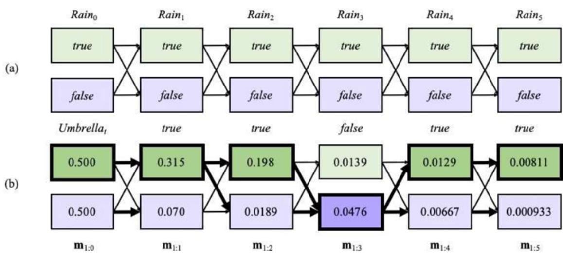
1. Possible state sequences for can be viewed as paths through a graph of the possible states at each time step. (States are shown as rectangles to avoid confusion with nodes in a Bayes net.) (b) Operation of the Viterbi algorithm for the umbrella observation sequence , where the evidence starts at time 1. For each , we have shown the values of the message , which gives the probability of the best sequence reaching each state at time . Also, for each state, the bold arrow leading into it indicates its best predecessor as measured by the product of the preceding sequence probability and the transition probability. Following the bold arrows back from the most likely state in gives the most likely sequence, shown by the bold outlines and darker shading.

Let’s focus in particular on paths that reach the state . Because of the Markov property, it follows that the most likely path to the state consists of the most likely path to some state at time 4 followed by a transition to ; and the state at time 4 that will become part of the path to is whichever maximizes the likelihood of that path. In other words, there is a recursive relationship between most likely paths to each state and most likely paths to each state .

We can use this property directly to construct a recursive algorithm for computing the most likely path given the evidence. We will use a recursively computed message , like the forward message in the filtering algorithm. The message is defined as follows: 5

5 Notice that these are not quite the probabilities of the most likely paths to reach the states given the evidence, which would be the conditional probabilities ; but the two vectors are related by a constant factor . The difference is immaterial because the MAX operator doesn’t care about constant factors. We get a slightly simpler recursion with defined this way.

\[\mathbf{m}\_{1:t} = \max\_{\mathbf{x}\_{1:t-1}} \mathbf{P} \left( \mathbf{x}\_{1:t-1}, \mathbf{X}\_t, \mathbf{e}\_{1:t} \right).\]

To obtain the recursive relationship between and , we can repeat more or less the same steps that we used for Equation (14.5) :

(14.11)

\[\begin{split} \mathbf{m}\_{1:t+1} &= \max\_{\mathbf{x}\_{1:t}} \mathbf{P}(\mathbf{x}\_{1:t}, \mathbf{X}\_{t+1}, \mathbf{e}\_{1:t+1}) = \max\_{\mathbf{x}\_{1:t}} \mathbf{P}(\mathbf{x}\_{1:t}, \mathbf{X}\_{t+1}, \mathbf{e}\_{1:t}, \mathbf{e}\_{t+1}) \\ &= \max\_{\mathbf{x}\_{1:t}} \mathbf{P}(e\_{t+1} | \mathbf{x}\_{1:t}, \mathbf{X}\_{t+1}, \mathbf{e}\_{1:t}) \mathbf{P}(\mathbf{x}\_{1:t}, \mathbf{X}\_{t+1}, \mathbf{e}\_{1:t}) \\ &= \mathbf{P}(e\_{t+1} | \mathbf{X}\_{t+1}) \max\_{\mathbf{x}\_{1:t}} \mathbf{P}(\mathbf{X}\_{t+1}, | \mathbf{x}\_{t}) P(\mathbf{x}\_{1:t}, \mathbf{e}\_{1:t}) \\ &= \mathbf{P}(e\_{t+1} | \mathbf{X}\_{t+1}) \max\_{\mathbf{x}\_t} \mathbf{P}(\mathbf{X}\_{t+1}, | \mathbf{x}\_t) \max\_{\mathbf{x}\_{1:t-1}} P(\mathbf{x}\_{1:t-1}, \mathbf{x}\_t, \mathbf{e}\_{1:t}) \end{split}\]

where the final term is exactly the entry for the particular state in the message vector . Equation (14.11) is essentially identical to the filtering equation (14.5) except that the summation over in Equation (14.5) is replaced by the maximization over in Equation (14.11) , and there is no normalization constant in Equation (14.11) . Thus, the algorithm for computing the most likely sequence is similar to filtering: it starts at time 0 with the prior and then runs forward along the sequence, computing the message at each time step using Equation (14.11) . The progress of this computation is shown in Figure 14.5(b) .

At the end of the observation sequence, will contain the probability for the most likely sequence reaching each of the final states. One can thus easily select the final state of the most likely sequence overall (the state outlined in bold at step 5). In order to identify the actual sequence, as opposed to just computing its probability, the algorithm will also need to record, for each state, the best state that leads to it; these are indicated by the bold arrows in Figure 14.5(b) . The optimal sequence is identified by following these bold arrows backwards from the best final state.

The algorithm we have just described is called the Viterbi algorithm, after its inventor, Andrew Viterbi. Like the filtering algorithm, its time complexity is linear in , the length of the sequence. Unlike filtering, which uses constant space, its space requirement is also linear in . This is because the Viterbi algorithm needs to keep the pointers that identify the best sequence leading to each state.

One final practical point: numerical underflow is a significant issue for the Viterbi algorithm. In Figure 14.5(b) , the probabilities are getting smaller and smaller—and this is just a toy

example. Real applications in DNA analysis or message decoding may have thousands or millions of steps. One possible solution is simply to normalize m at each step; this rescaling does not affect correctness because . A second solution is to use log probabilities everywhere and replace multiplication by addition. Again, correctness is unaffected because the log function is monotonic, so .

14.3 Hidden Markov Models

The preceding section developed algorithms for temporal probabilistic reasoning using a general framework that was independent of the specific form of the transition and sensor models and independent of the nature of the state and evidence variables. In this and the next two sections, we discuss more concrete models and applications that illustrate the power of the basic algorithms and in some cases allow further improvements.

We begin with the hidden Markov model, or HMM. An HMM is a temporal probabilistic model in which the state of the process is described by a single, discrete random variable. The possible values of the variable are the possible states of the world. The umbrella example described in the preceding section is therefore an HMM, since it has just one state variable: . What happens if you have a model with two or more state variables? You can still fit it into the HMM framework by combining the variables into a single “megavariable” whose values are all possible tuples of values of the individual state variables. We will see that the restricted structure of HMMs allows for a simple and elegant matrix implementation of all the basic algorithms. 6

6 The reader unfamiliar with basic operations on vectors and matrices might wish to consult Appendix A before proceeding with this section.

Hidden Markov model

Although HMMs require the state to be a single, discrete variable, there is no corresponding restriction on the evidence variables. This is because the evidence variables are always observed, which means that there is no need to keep track of any distribution over their values. (If a variable is not observed, it can simply be dropped from the model for that time step.) There can be many evidence variables, both discrete and continuous.

14.3.1 Simplified matrix algorithms

With a single, discrete state variable , we can give concrete form to the representations of the transition model, the sensor model, and the forward and backward messages. Let the state variable have values denoted by integers , where is the number of possible states. The transition model becomes an matrix T, where

\[\mathbf{T}\_{ij} = P(X\_t = j | X\_{t-1} = i).\]

That is, is the probability of a transition from state to state . For example, if we number the states and as 1 and 2, respectively, then the transition matrix for the umbrella world defined in Figure 14.2 is

\[\mathbf{T} = \mathbf{P}(X\_t | X\_{t-1}) = \begin{pmatrix} 0.7 & 0.3\\ 0.3 & 0.7 \end{pmatrix}.\]

We also put the sensor model in matrix form. In this case, because the value of the evidence variable is known at time (call it ), we need only specify, for each state, how likely it is that the state causes to appear: we need for each state . For mathematical convenience we place these values into an diagonal observation matrix, , one for each time step. The th diagonal entry of is and the other entries are 0. For example, on day 1 in the umbrella world of Figure 14.5 , , and on day 3, , so we have

\[\mathbf{O}\_1 = \begin{pmatrix} 0.9 & 0\\ 0 & 0.2 \end{pmatrix}; \qquad \mathbf{O}\_3 = \begin{pmatrix} 0.1 & 0\\ 0 & 0.8 \end{pmatrix}.\]

Now, if we use column vectors to represent the forward and backward messages, all the computations become simple matrix–vector operations. The forward equation (14.5) becomes

(14.12)

\[\mathbf{f}\_{1:t+1} = \alpha \mathbf{O}\_{t+1} \mathbf{T}^\top \mathbf{f}\_{1:t}\]

and the backward equation (14.9) becomes

(14.13)

\[\mathbf{b}\_{k+1:t} = \mathbf{T} \mathbf{O}\_{k+1} \mathbf{b}\_{k+2:t}.\]

From these equations, we can see that the time complexity of the forward–backward algorithm (Figure 14.4 ) applied to a sequence of length is , because each step requires multiplying an -element vector by an matrix. The space requirement is , because the forward pass stores vectors of size .

Besides providing an elegant description of the filtering and smoothing algorithms for HMMs, the matrix formulation reveals opportunities for improved algorithms. The first is a simple variation on the forward–backward algorithm that allows smoothing to be carried out in constant space, independently of the length of the sequence. The idea is that smoothing for any particular time slice requires the simultaneous presence of both the forward and backward messages, and , according to Equation (14.8) . The forward–backward algorithm achieves this by storing the s computed on the forward pass so that they are available during the backward pass. Another way to achieve this is with a single pass that propagates both and b in the same direction. For example, the “forward” message can be propagated backward if we manipulate Equation (14.12) to work in the other direction:

\[\mathbf{f}\_{1:t} = \alpha'(\mathbf{f}^\top)^{-1} \mathbf{O}\_{t+1}^{-1} \mathbf{f}\_{1:t+1}.\]

The modified smoothing algorithm works by first running the standard forward pass to compute (forgetting all the intermediate results) and then running the backward pass for both b and f together, using them to compute the smoothed estimate at each step. Since only one copy of each message is needed, the storage requirements are constant (i.e., independent of , the length of the sequence). There are two significant restrictions on this algorithm: it requires that the transition matrix be invertible and that the sensor model have no zeroes—that is, that every observation be possible in every state.

A second area in which the matrix formulation reveals an improvement is in online smoothing with a fixed lag. The fact that smoothing can be done in constant space suggests that there should exist an efficient recursive algorithm for online smoothing—that is, an algorithm whose time complexity is independent of the length of the lag. Let us suppose that the lag is ; that is, we are smoothing at time slice , where the current time is . By Equation (14.8) , we need to compute

\[ \alpha \mathbf{f}\_{1:t-d} \times \mathbf{b}\_{t-d+1:t} \]

for slice . Then, when a new observation arrives, we need to compute

\[ \alpha \mathbf{f}\_{1:t-d+1} \times \mathbf{b}\_{t-d+2:t+1} \]

for slice . How can this be done incrementally? First, we can compute from , using the standard filtering process, Equation (14.5) .

Computing the backward message incrementally is trickier, because there is no simple relationship between the old backward message and the new backward message . Instead, we will examine the relationship between the old backward message and the backward message at the front of the sequence, . To do this, we apply Equation (14.13) times to get

(14.14)

\[\mathbf{b}\_{t-d+1:t} = \left(\prod\_{i=t-d+1}^{t} \mathbf{T} \mathbf{O}\_{i}\right) \mathbf{b}\_{t+1:t} = \mathbf{B}\_{t-d+1:t} \mathbf{1}\_{t}\]

where the matrix is the product of the sequence of T and O matrices and 1 is a vector of 1s. B can be thought of as a “transformation operator” that transforms a later backward message into an earlier one. A similar equation holds for the new backward messages after the next observation arrives:

(14.15)

\[\mathbf{b}\_{t-d+2:t+1} = \left(\prod\_{i=t-d+2}^{t+1} \mathbf{TO}\_i\right) \mathbf{b}\_{t+2:t+1} = \mathbf{B}\_{t-d+2:t+1} \mathbf{1}.\]

Examining the product expressions in Equations (14.14) and (14.15) , we see that they have a simple relationship: to get the second product, “divide” the first product by the first element , and multiply by the new last element . In matrix language, then, there is a simple relationship between the old and new B matrices:

(14.16)

\[\mathbf{B}\_{t-d+2:t+1} = \mathbf{O}\_{t-d+1}^{-1} \mathbf{T}^{-1} \mathbf{B}\_{t-d+1:t} \mathbf{T} \mathbf{O}\_{t+1}.\]

This equation provides an incremental update for the B matrix, which in turn (through Equation (14.15) ) allows us to compute the new backward message . The complete algorithm, which requires storing and updating and B, is shown in Figure 14.6 .

Figure 14.6

An algorithm for smoothing with a fixed time lag of steps, implemented as an online algorithm that outputs the new smoothed estimate given the observation for a new time step. Notice that the final output is just , by Equation (14.14) .

14.3.2 Hidden Markov model example: Localization

On page 133, we introduced a simple form of the localization problem for the vacuum world. In that version, the robot had a single nondeterministic Move action and its sensors reported perfectly whether or not obstacles lay immediately to the north, south, east, and west; the robot’s belief state was the set of possible locations it could be in.

Here we make the problem slightly more realistic by allowing for noise in the sensors, and formalizing the idea that the robot moves randomly—it is equally likely to move to any adjacent empty square. The state variable represents the location of the robot on the discrete grid; the domain of this variable is the set of empty squares, which we will label by the . Let NEIGHBORS be the set of empty squares that are adjacent to and let be the size of that set. Then the transition model for the Move action says that the robot is equally likely to end up at any neighboring square:

\[P(X\_{t+1} = j | X\_t = i) = \mathbf{T}\_{ij} = \begin{cases} 1/N(i) \text{ if } j \in \text{NEGBours} \,(i),\\ 0 \text{ otherwise.} \end{cases}\]

We don’t know where the robot starts, so we will assume a uniform distribution over all the squares; that is, . For the particular environment we consider (Figure 14.7 ), and the transition matrix has entries.

Posterior distribution over robot location: (a) after one observation (i.e., obstacles to the north, south, and west); (b) after a random move to an adjacent location and a second observation (i.e., obstacles to the north and south). The size of each disk corresponds to the probability that the robot is at that location. The sensor error rate for each bit is .

The sensor variable has 16 possible values, each a four-bit sequence giving the presence or absence of an obstacle in each of the compass directions NESW. For example, means that the north and south sensors report an obstacle and the east and west do not. Suppose

that each sensor’s error rate is and that errors occur independently for the four sensor directions. In that case, the probability of getting all four bits right is and the probability of getting them all wrong is . Furthermore, if is the discrepancy—the number of bits that are different—between the true values for square and the actual reading , then the probability that a robot in square would receive a sensor reading is

\[P(E\_t = e\_t | X\_t = i) = (\mathbf{O}\_t)\_{ii} = (1 - \epsilon)^{4 - d\_{it}} \epsilon^{d\_{it}}.\]

For example, the probability that a square with obstacles to the north and south would produce a sensor reading is .

Given the matrices T and , the robot can use Equation (14.12) to compute the posterior distribution over locations—that is, to work out where it is. Figure 14.7 shows the distributions and . This is the same maze we saw before in Figure 4.18 (page 134), but there we used logical filtering to find the locations that were possible, assuming perfect sensing. Those same locations are still the most likely with noisy sensing, but now every location has some nonzero probability because any location could produce any sensor values.

In addition to filtering to estimate its current location, the robot can use smoothing (Equation (14.13) ) to work out where it was at any given past time—for example, where it began at time 0—and it can use the Viterbi algorithm to work out the most likely path it has taken to get where it is now. Figure 14.8 shows the localization error and Viterbi path error for various values of the per-bit sensor error rate . Even when is —which means that the overall sensor reading is wrong 59% of the time—the robot is usually able to work out its location to within two squares after 20 observations. This is because of the algorithm’s ability to integrate evidence over time and to take into account the probabilistic constraints imposed on the location sequence by the transition model. When is or less, the robot needs only a few observations to work out where it is and to track its position accurately. When is , both the localization error and the Viterbi path error remain large; in other words, the robot is lost. This is because a sensor with an error probability of provides too little information to counteract the loss of information about the robot’s position that comes from the unpredictable random motion.

Performance of HMM localization as a function of the length of the observation sequence for various different values of the sensor error probability ; data averaged over 400 runs. (a) The localization error, defined as the Manhattan distance from the true location. (b) The Viterbi path error, defined as the average Manhattan distance of states on the Viterbi path from corresponding states on the true path.

The state variable for the example we have considered in this section is a physical location in the world. Other problems can, of course, include other aspects of the world. Exercise 14.ROOM asks you to consider a version of the vacuum robot that has the policy of going straight for as long as it can; only when it encounters an obstacle does it change to a new heading. To model this robot, each state in the model consists of a (location, heading) pair. For the environment in Figure 14.7 , which has 42 empty squares, this leads to 168 states and a transition matrix with entries—still a manageable number.

If we add the possibility of dirt in each of the 42 squares, the number of states is multiplied by and the transition matrix has more than entries—no longer a manageable number. In general, if the state is composed of discrete variables with at most values each, the corresponding HMM transition matrix will have size and the per-update computation time will also be .

For these reasons, although HMMs have many uses in areas ranging from speech recognition to molecular biology, they are fundamentally limited in their ability to represent complex processes. In the terminology introduced in Chapter 2 , HMMs are an atomic representation: states of the world have no internal structure and are simply labeled by integers. Section 14.5 shows how to use dynamic Bayesian networks—a factored representation—to model domains with many state variables. The next section shows how to handle domains with continuous state variables, which of course lead to an infinite state space.

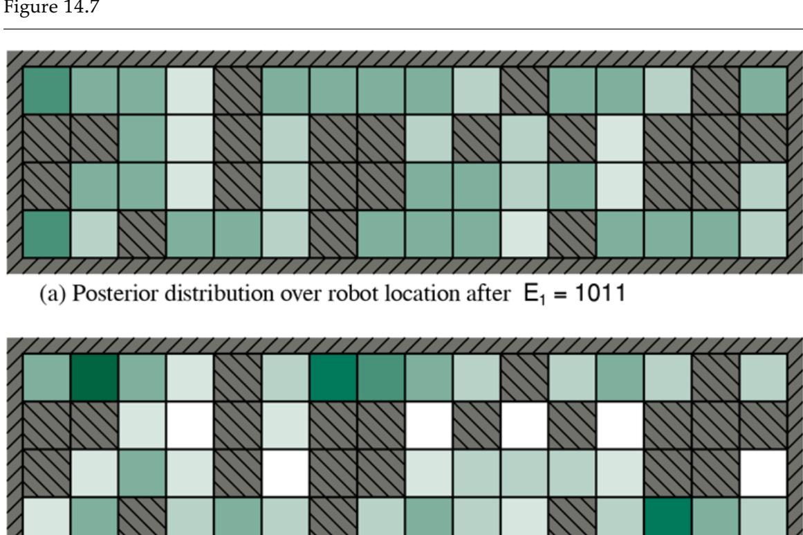
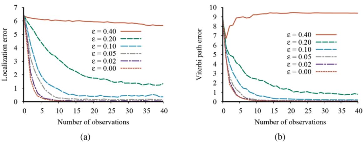
14.4 Kalman Filters

Imagine watching a small bird flying through dense jungle foliage at dusk: you glimpse brief, intermittent flashes of motion; you try hard to guess where the bird is and where it will appear next so that you don’t lose it. Or imagine that you are a World War II radar operator peering at a faint, wandering blip that appears once every 10 seconds on the screen. Or, going back further still, imagine you are Kepler trying to reconstruct the motions of the planets from a collection of highly inaccurate angular observations taken at irregular and imprecisely measured intervals.

In all these cases, you are doing filtering: estimating state variables (here, the position and velocity of a moving object) from noisy observations over time. If the variables were discrete, we could model the system with a hidden Markov model. This section examines methods for handling continuous variables, using an algorithm called Kalman filtering, after one of its inventors, Rudolf Kalman.

Kalman filtering

The bird’s flight might be specified by six continuous variables at each time point; three for position and three for velocity . We will need suitable conditional densities to represent the transition and sensor models; as in Chapter 13 , we will use linear–Gaussian distributions. This means that the next state must be a linear function of the current state , plus some Gaussian noise, a condition that turns out to be quite reasonable in practice. Consider, for example, the -coordinate of the bird, ignoring the other coordinates for now. Let the time interval between observations be , and assume constant velocity during the interval; then the position update is given by . Adding Gaussian noise (to account for wind variation, etc.), we obtain a linear–Gaussian transition model:

\[P(X\_{t+\Delta} = x\_{t+\Delta} | X\_t = x\_t, \dot{X}\_t = \dot{x}\_t) = N(x\_{t+\Delta}; x\_t + \dot{x}\_t \Delta, \sigma^2).\]

The Bayesian network structure for a system with position vector and velocity is shown in Figure 14.9 . Note that this is a very specific form of linear–Gaussian model; the general form will be described later in this section and covers a vast array of applications beyond the simple motion examples of the first paragraph. The reader might wish to consult Appendix A for some of the mathematical properties of Gaussian distributions; for our immediate purposes, the most important is that a multivariate Gaussian distribution for variables is specified by a -element mean and a covariance matrix .

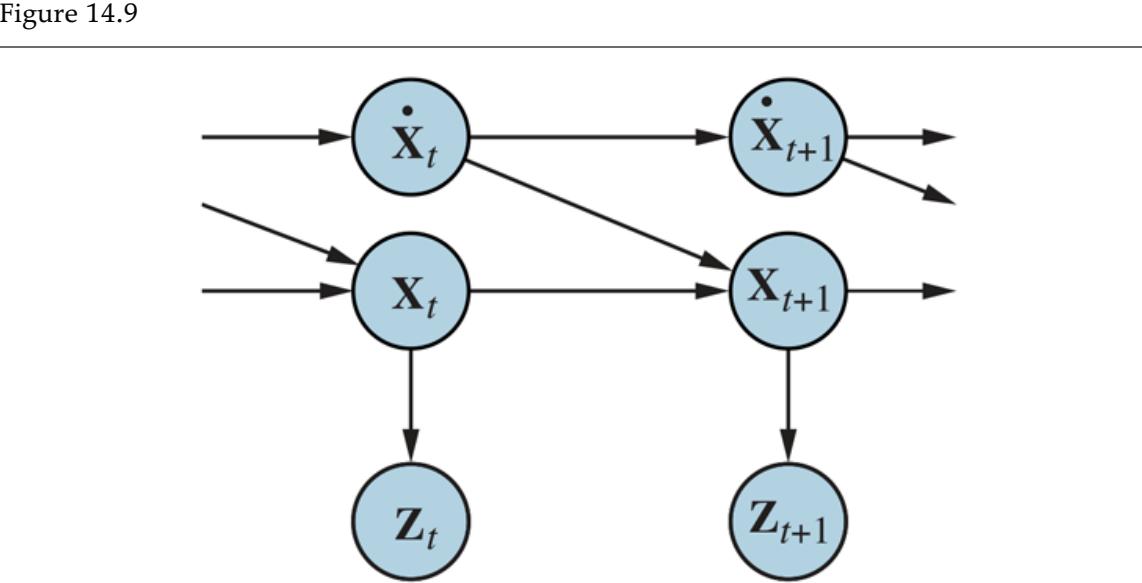
Bayesian network structure for a linear dynamical system with position , velocity , and position measurement .

14.4.1 Updating Gaussian distributions

In Chapter 13 on page 423, we alluded to a key property of the linear–Gaussian family of distributions: it remains closed under Bayesian updating. (That is, given any evidence, the posterior is still in the linear–Gaussian family.) Here we make this claim precise in the context of filtering in a temporal probability model. The required properties correspond to the two-step filtering calculation in Equation (14.5) :

1. If the current distribution is Gaussian and the transition model is linear–Gaussian, then the one-step predicted distribution given by (14.17)

\[\mathbf{P}(\mathbf{X}\_{t+1}|\mathbf{e}\_{1:t}) = \int\_{\mathbf{x}\_{t}} \mathbf{P}(\mathbf{X}\_{t+1}|\mathbf{x}\_{t}) P(\mathbf{x}\_{t}|\mathbf{e}\_{1:t}) d\mathbf{x}\_{t}\]

is also a Gaussian distribution.

2. If the prediction is Gaussian and the sensor model is linear–Gaussian, then, after conditioning on the new evidence, the updated distribution

(14.18)

\[\mathbf{P}(\mathbf{X}\_{t+1}|\mathbf{e}\_{1:t+1}) = \alpha \mathbf{P}(\mathbf{e}\_{t+1}|\mathbf{X}\_{t+1})\mathbf{P}(\mathbf{X}\_{t+1}|\mathbf{e}\_{1:t})\]

is also a Gaussian distribution.

Thus, the operator for Kalman filtering takes a Gaussian forward message , specified by a mean and covariance , and produces a new multivariate Gaussian forward message , specified by a mean and covariance . So if we start with a Gaussian prior , filtering with a linear–Gaussian model produces a Gaussian state distribution for all time.

This seems to be a nice, elegant result, but why is it so important? The reason is that except for a few special cases such as this, filtering with continuous or hybrid (discrete and continuous) networks generates state distributions whose representation grows without bound over time. This statement is not easy to prove in general, but Exercise 14.KFSW shows what happens for a simple example.

14.4.2 A simple one-dimensional example

We have said that the FORWARD operator for the Kalman filter maps a Gaussian into a new Gaussian. This translates into computing a new mean and covariance from the previous mean and covariance. Deriving the update rule in the general (multivariate) case requires rather a lot of linear algebra, so we will stick to a very simple univariate case for now, and later give the results for the general case. Even for the univariate case, the calculations are somewhat tedious, but we feel that they are worth seeing because the usefulness of the Kalman filter is tied so intimately to the mathematical properties of Gaussian distributions.

The temporal model we consider describes a random walk of a single continuous state variable with a noisy observation . An example might be the “consumer confidence” index, which can be modeled as undergoing a random Gaussian-distributed change each month and is measured by a random consumer survey that also introduces Gaussian sampling noise. The prior distribution is assumed to be Gaussian with variance :

\[P(x\_0) = \alpha e^{-\frac{1}{2}\left(\frac{(x\_0 - \mu\_0)^2}{\sigma\_0^2}\right)}\]

(For simplicity, we use the same symbol for all normalizing constants in this section.) The transition model adds a Gaussian perturbation of constant variance to the current state:

\[P(x\_{t+1}|x\_t) = \alpha e^{-\frac{1}{2}\left(\frac{(x\_{t+1} - x\_t)^2}{\sigma\_x^2}\right)}\]

The sensor model assumes Gaussian noise with variance :

\[P(z\_t|x\_t) = \alpha e^{-\frac{1}{2}\left(\frac{(z\_t - x\_t)^2}{\sigma\_z^2}\right)}.\]

Now, given the prior , the one-step predicted distribution comes from Equation (14.17) :

\[\begin{split} P(x\_1) &= \int\_{-\infty}^{\infty} P(x\_1|x\_0)P(x\_0)dx\_0 = \alpha \int\_{-\infty}^{\infty} e^{-\frac{1}{2}\left(\frac{(x\_1 - x\_0)^2}{\sigma\_x^2}\right)} e^{-\frac{1}{2}\left(\frac{(x\_0 - \mu\_0)^2}{\sigma\_0^2}\right)} dx\_0 \\ &= \alpha \int\_{-\infty}^{\infty} e^{-\frac{1}{2}\left(\frac{\sigma\_0^2 (x\_1 - x\_0)^2 + \sigma\_x^2 (x\_0 - \mu\_0)^2}{\sigma\_0^2 \sigma\_x^2}\right)} dx\_0. \end{split}\]

This integral looks rather complicated. The key to progress is to notice that the exponent is the sum of two expressions that are quadratic in and hence is itself a quadratic in . A simple trick known as completing the square allows the rewriting of any quadratic as the sum of a squared term and a residual term that is independent of . In this case, we have , , and . The residual term can be taken outside the integral, giving us

\[P(x\_1) = \alpha e^{-\frac{1}{2}\left(c - \frac{b^2}{4\epsilon}\right)} \int\_{-\infty}^{\infty} e^{-\frac{1}{2}\left(a(x\_0 - \frac{-b}{x\_0})^2\right)} dx\_0.\]

Completing the square

Now the integral is just the integral of a Gaussian over its full range, which is simply 1. Thus, we are left with only the residual term from the quadratic. Plugging back in the expressions for , , and and simplifying, we obtain

\[P(x\_1) = \alpha e^{-\frac{1}{2} \left(\frac{(x\_1 - \mu\_0)^2}{\sigma\_0^2 + \sigma\_0^2}\right)}.\]

That is, the one-step predicted distribution is a Gaussian with the same mean and a variance equal to the sum of the original variance and the transition variance .

To complete the update step, we need to condition on the observation at the first time step, namely, . From Equation (14.18) , this is given by

\[\begin{aligned} P(x\_1|z\_1) &= \alpha P(z\_1|x\_1)P(x\_1) \\ &= \alpha e^{-\frac{1}{2}\left(\frac{(z\_1-x\_1)^2}{\sigma\_z^2}\right)} e^{-\frac{1}{2}\left(\frac{(x\_1-\mu\_0)^2}{\sigma\_0^2 + \sigma\_x^2}\right)} \end{aligned}\]

Once again, we combine the exponents and complete the square (Exercise 14.KALM), obtaining the following expression for the posterior:

\[(\clubsuit 4.19)\]

\[P(x\_1|z\_1) = \alpha e^{-\frac{1}{2} \frac{\left(x\_1 - \frac{(\sigma\_0^2 + \sigma\_x^2)z\_1 + \sigma\_x^2 \mu\_0}{\sigma\_0^2 + \sigma\_x^2 + \sigma\_x^2}\right)}{\frac{1}{2} \frac{(\sigma\_0^2 + \sigma\_x^2)\sigma\_0^2 / (\sigma\_0^2 + \sigma\_x^2 + \sigma\_x^2)}{(\sigma\_0^2 + \sigma\_x^2) / (\sigma\_0^2 + \sigma\_x^2 + \sigma\_x^2)}}.\]

Thus, after one update cycle, we have a new Gaussian distribution for the state variable.

From the Gaussian formula in Equation (14.19) , we see that the new mean and standard deviation can be calculated from the old mean and standard deviation as follows:

(14.20)

\[\mu\_{t+1} = \frac{(\sigma\_t^2 + \sigma\_x^2)z\_{t+1} + \sigma\_z^2\mu\_t}{\sigma\_t^2 + \sigma\_x^2 + \sigma\_z^2} \qquad \text{and} \qquad \sigma\_{t+1}^2 = \frac{(\sigma\_t^2 + \sigma\_x^2)\sigma\_z^2}{\sigma\_t^2 + \sigma\_x^2 + \sigma\_z^2}.\]

Figure 14.10 shows one update cycle of the Kalman filter in the one-dimensional case for particular values of the transition and sensor models.

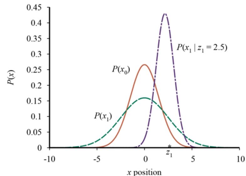
Stages in the Kalman filter update cycle for a random walk with a prior given by and , transition noise given by , sensor noise given by , and a first observation (marked on the -axis). Notice how the prediction is flattened out, relative to , by the transition noise. Notice also that the mean of the posterior distribution is slightly to the left of the observation because the mean is a weighted average of the prediction and the observation.

Equation (14.20) plays exactly the same role as the general filtering equation (14.5) or the HMM filtering equation (14.12) . Because of the special nature of Gaussian distributions, however, the equations have some interesting additional properties.

First, we can interpret the calculation for the new mean as a weighted mean of the new observation and the old mean . If the observation is unreliable, then is large and we pay more attention to the old mean; if the old mean is unreliable ( is large) or the process is highly unpredictable ( is large), then we pay more attention to the observation.

Second, notice that the update for the variance is independent of the observation. We can therefore compute in advance what the sequence of variance values will be. Third, the sequence of variance values converges quickly to a fixed value that depends only on and , thereby substantially simplifying the subsequent calculations. (See Exercise 14.VARI.)

14.4.3 The general case

The preceding derivation illustrates the key property of Gaussian distributions that allows Kalman filtering to work: the fact that the exponent is a quadratic form. This is true not just for the univariate case; the full multivariate Gaussian distribution has the form

\[N(\mathbf{x}; \mu, \Sigma) = \alpha e^{-\frac{1}{2}\left( (\mathbf{x} - \mu)^{\top} \Sigma^{-1} (\mathbf{x} - \mu) \right)}.\]

Multiplying out the terms in the exponent, we see that the exponent is also a quadratic function of the values in x. Thus, filtering preserves the Gaussian nature of the state distribution.

Let us first define the general temporal model used with Kalman filtering. Both the transition model and the sensor model are required to be a linear transformation with additive Gaussian noise. Thus, we have

(14.21)

\[\begin{array}{rcl}P(\mathbf{x}\_{t+1}|\mathbf{x}\_{t})&=&N(\mathbf{x}\_{t+1};\mathbf{F}\mathbf{x}\_{t},\Sigma\_{x}),\\P(\mathbf{z}\_{t}|\mathbf{x}\_{t})&=&N(\mathbf{z}\_{t};\mathbf{H}\mathbf{x}\_{t},\Sigma\_{z}),\end{array}\]

where F and are matrices describing the linear transition model and transition noise covariance, and H and are the corresponding matrices for the sensor model. Now the update equations for the mean and covariance, in their full, hairy horribleness, are

(14.22)

\[\begin{array}{rcl}\mu\_{t+1} &=& \mathbf{F}\mu\_{t} + \mathbf{K}\_{t+1}(\mathbf{z}\_{t+1} - \mathbf{H}\mathbf{F}\mu\_{t})\\\Sigma\_{t+1} &=& (\mathbf{I} - \mathbf{K}\_{t+1}\mathbf{H})(\mathbf{F}\Sigma\_{t}\mathbf{F}^{\top} + \Sigma\_{x}),\end{array}\]

Kalman gain matrix

where is the Kalman gain matrix. Believe it or not, these equations make some intuitive sense. For example, consider the update for the mean state estimate . The term is the predicted state at , so is the predicted observation. Therefore, the term represents the error in the predicted observation. This is multiplied by to correct the predicted state; hence, is a measure of how seriously to take the new observation relative to the prediction. As in Equation (14.20) , we also have the property that the variance update is independent of the observations. The sequence of values for and can therefore be computed offline, and the actual calculations required during online tracking are quite modest.

To illustrate these equations at work, we have applied them to the problem of tracking an object moving on the – plane. The state variables are , so , , , and are matrices. Figure 14.11(a) shows the true trajectory, a series of noisy observations, and the trajectory estimated by Kalman filtering, along with the covariances indicated by the one-standard-deviation contours. The filtering process does a good job of tracking the actual motion, and, as expected, the variance quickly reaches a fixed point.

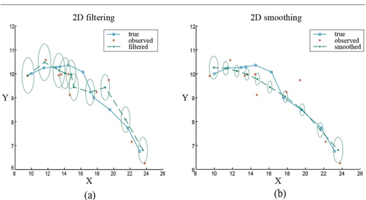
1. Results of Kalman filtering for an object moving on the – plane, showing the true trajectory (left to right), a series of noisy observations, and the trajectory estimated by Kalman filtering. Variance in the position estimate is indicated by the ovals. (b) The results of Kalman smoothing for the same observation sequence.

We can also derive equations for smoothing as well as filtering with linear–Gaussian models. The smoothing results are shown in Figure 14.11(b) . Notice how the variance in the position estimate is sharply reduced, except at the ends of the trajectory (why?), and that the estimated trajectory is much smoother.

14.4.4 Applicability of Kalman filtering

The Kalman filter and its elaborations are used in a vast array of applications. The “classical” application is in radar tracking of aircraft and missiles. Related applications include acoustic tracking of submarines and ground vehicles and visual tracking of vehicles and people. In a slightly more esoteric vein, Kalman filters are used to reconstruct particle trajectories from bubble-chamber photographs and ocean currents from satellite surface measurements. The range of application is much larger than just the tracking of motion: any system characterized by continuous state variables and noisy measurements will do. Such systems include pulp mills, chemical plants, nuclear reactors, plant ecosystems, and national economies.

Extended Kalman filter (EKF)

Nonlinear

The fact that Kalman filtering can be applied to a system does not mean that the results will be valid or useful. The assumptions made—linear–Gaussian transition and sensor models are very strong. The extended Kalman filter (EKF) attempts to overcome nonlinearities in the system being modeled. A system is nonlinear if the transition model cannot be described as a matrix multiplication of the state vector, as in Equation (14.21) . The EKF works by modeling the system as locally linear in in the region of , the mean of the current state distribution. This works well for smooth, well-behaved systems and allows the tracker to maintain and update a Gaussian state distribution that is a reasonable approximation to the true posterior. A detailed example is given in Chapter 26 .

What does it mean for a system to be “unsmooth” or “poorly behaved”? Technically, it means that there is significant nonlinearity in system response within the region that is “close” (according to the covariance ) to the current mean . To understand this idea in nontechnical terms, consider the example of trying to track a bird as it flies through the jungle. The bird appears to be heading at high speed straight for a tree trunk. The Kalman

filter, whether regular or extended, can make only a Gaussian prediction of the location of the bird, and the mean of this Gaussian will be centered on the trunk, as shown in Figure 14.12(a) . A reasonable model of the bird, on the other hand, would predict evasive action to one side or the other, as shown in Figure 14.12(b) . Such a model is highly nonlinear, because the bird’s decision varies sharply depending on its precise location relative to the trunk.

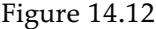
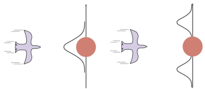
A bird flying toward a tree (top views). (a) A Kalman filter will predict the location of the bird using a single Gaussian centered on the obstacle. (b) A more realistic model allows for the bird’s evasive action, predicting that it will fly to one side or the other.

To handle examples like these, we clearly need a more expressive language for representing the behavior of the system being modeled. Within the control theory community, for which problems such as evasive maneuvering by aircraft raise the same kinds of difficulties, the standard solution is the switching Kalman filter. In this approach, multiple Kalman filters run in parallel, each using a different model of the system—for example, one for straight flight, one for sharp left turns, and one for sharp right turns. A weighted sum of predictions is used, where the weight depends on how well each filter fits the current data. We will see in the next section that this is simply a special case of the general dynamic Bayesian network model, obtained by adding a discrete “maneuver” state variable to the network shown in Figure 14.9 . Switching Kalman filters are discussed further in Exercise 14.KFSW.

Switching Kalman filter

14.5 Dynamic Bayesian Networks

Dynamic Bayesian networks, or DBNs, extend the semantics of standard Bayesian networks to handle temporal probability models of the kind described in Section 14.1 . We have already seen examples of DBNs: the umbrella network in Figure 14.2 and the Kalman filter network in Figure 14.9 . In general, each slice of a DBN can have any number of state variables and evidence variables . For simplicity, we assume that the variables, their links, and their conditional distributions are exactly replicated from slice to slice and that the DBN represents a first-order Markov process, so that each variable can have parents only in its own slice or the immediately preceding slice. In this way, the DBN corresponds to a Bayesian network with infinitely many variables.

Dynamic Bayesian network

It should be clear that every hidden Markov model can be represented as a DBN with a single state variable and a single evidence variable. It is also the case that every discretevariable DBN can be represented as an HMM; as explained in Section 14.3 , we can combine all the state variables in the DBN into a single state variable whose values are all possible tuples of values of the individual state variables. Now, if every HMM is a DBN and every DBN can be translated into an HMM, what’s the difference? The difference is that, by decomposing the state of a complex system into its constituent variables, we can take advantage of sparseness in the temporal probability model.

To see what this means in practice, remember that in Section 14.3 we said that an HMM representation for a temporal process with discrete variables, each with up to values, needs a transition matrix of size . The DBN representation, on the other hand, has size if the number of parents of each variable is bounded by . In other words, the DBN representation is linear rather than exponential in the number of variables. For the vacuum robot with 42 possibly dirty locations, the number of probabilities required is reduced from to a few thousand.

We have already explained that every Kalman filter model can be represented in a DBN with continuous variables and linear–Gaussian conditional distributions (Figure 14.9 ). It should be clear from the discussion at the end of the preceding section that not every DBN can be represented by a Kalman filter model. In a Kalman filter, the current state distribution is always a single multivariate Gaussian distribution—that is, a single “bump” in a particular location. DBNs, on the other hand, can model arbitrary distributions.

For many real-world applications, this flexibility is essential. Consider, for example, the current location of my keys. They might be in my pocket, on the bedside table, on the kitchen counter, dangling from the front door, or locked in the car. A single Gaussian bump that included all these places would have to allocate significant probability to the keys being in mid-air above the front garden. Aspects of the real world such as purposive agents, obstacles, and pockets introduce “nonlinearities” that require combinations of discrete and continuous variables in order to get reasonable models.

14.5.1 Constructing DBNs

To construct a DBN, one must specify three kinds of information: the prior distribution over the state variables, ; the transition model ; and the sensor model . To specify the transition and sensor models, one must also specify the topology of the connections between successive slices and between the state and evidence variables. Because the transition and sensor models are assumed to be time-homogeneous—the same for all —it is most convenient simply to specify them for the first slice. For example, the complete DBN specification for the umbrella world is given by the three-node network shown in Figure 14.13(a) . From this specification, the complete DBN with an unbounded number of time slices can be constructed as needed by copying the first slice.

Figure 14.13

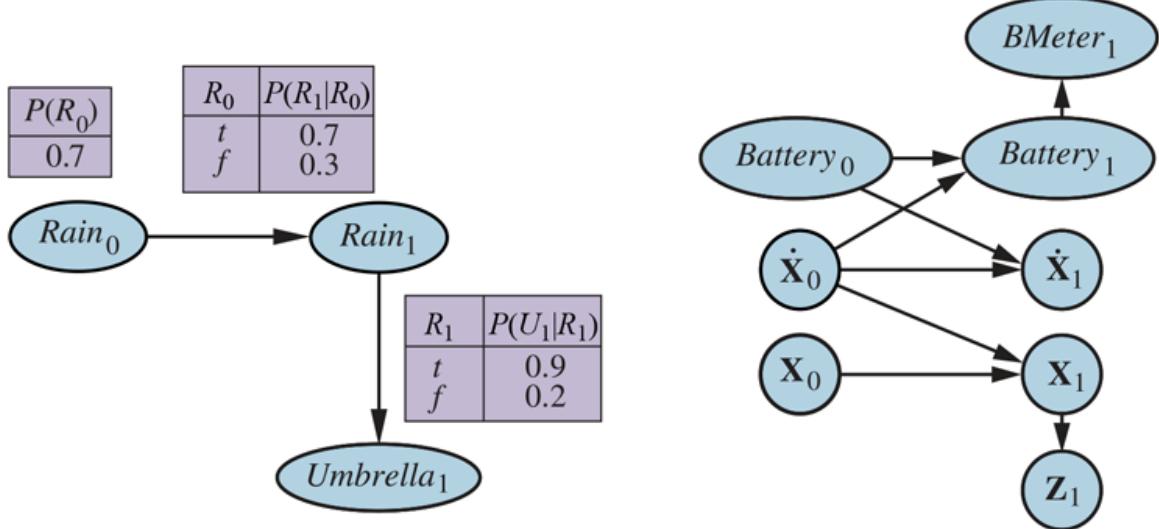
Left: Specification of the prior, transition model, and sensor model for the umbrella DBN. Subsequent slices are copies of slice 1. Right: A simple DBN for robot motion in the plane.

Let us now consider a more interesting example: monitoring a battery-powered robot moving in the X–Y plane, as introduced at the end of Section 14.1 . First, we need state variables, which will include both for position and for velocity. We assume some method of measuring position—perhaps a fixed camera or onboard GPS (Global Positioning System)—yielding measurements . The position at the next time step depends on the current position and velocity, as in the standard Kalman filter model. The velocity at the next step depends on the current velocity and the state of the battery. We add to represent the actual battery charge level, which has as parents the previous battery level and the velocity, and we add , which measures the battery charge level. This gives us the basic model shown in Figure 14.13(b) .

It is worth looking in more depth at the nature of the sensor model for . Let us suppose, for simplicity, that both and can take on discrete values 0 through 5. (Exercise 14.BATT asks you to relate this discrete model to a corresponding continuous model.) If the meter is always accurate, then the CPT should have probabilities of 1.0 “along the diagonal” and probabilities of 0.0 elsewhere. In reality, noise always creeps into measurements. For continuous measurements, a Gaussian distribution with a small variance might be used. For our discrete variables, we can approximate a Gaussian using a distribution in which the probability of error drops off in the appropriate way, so that the probability of a large error is very small. We use the term Gaussian error model to cover both the continuous and discrete versions. 7

7 Strictly speaking, a Gaussian distribution is problematic because it assigns nonzero probability to large negative charge levels. The beta distribution is sometimes a better choice for a variable whose range is restricted.

Anyone with hands-on experience of robotics, computerized process control, or other forms of automatic sensing will readily testify to the fact that small amounts of measurement noise are often the least of one’s problems. Real sensors fail. When a sensor fails, it does not necessarily send a signal saying, “Oh, by the way, the data I’m about to send you is a load of nonsense.” Instead, it simply sends the nonsense. The simplest kind of failure is called a transient failure, where the sensor occasionally decides to send some nonsense. For example, the battery level sensor might have a habit of sending a reading of 0 when someone bumps the robot, even if the battery is fully charged.

Gaussian error model

Let’s see what happens when a transient failure occurs with a Gaussian error model that doesn’t accommodate such failures. Suppose, for example, that the robot is sitting quietly and observes 20 consecutive battery readings of 5. Then the battery meter has a temporary seizure and the next reading is . What will the simple Gaussian error model lead us to believe about ? According to Bayes’ rule, the answer depends on both the sensor model and the prediction . If the probability of a large sensor error is significantly less than the probability of a transition to , even if the latter is very unlikely, then the posterior distribution will assign a high probability to the battery’s being empty.

Transient failure

A second reading of 0 at will make this conclusion almost certain. If the transient failure then disappears and the reading returns to 5 from onwards, the estimate for the battery level will quickly return to 5. (This does not mean the algorithm thinks the battery magically recharged itself, which may be physically impossible; instead, the

algorithm now believes that the battery was never low and the extremely unlikely hypothesis that the battery meter had two consecutive huge errors must be the right explanation.) This course of events is illustrated in the upper curve of Figure 14.14(a) , which shows the expected value (see Appendix A ) of over time, using a discrete Gaussian error model.

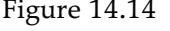
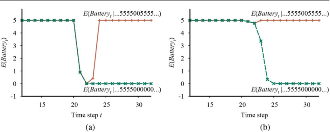
1. Upper curve: trajectory of the expected value of for an observation sequence consisting of all 5s except for 0s at and , using a simple Gaussian error model. Lower curve: trajectory when the observation remains at 0 from onwards. (b) The same experiment run with the transient failure model. The transient failure is handled well, but the persistent failure results in excessive pessimism about the battery charge.

Despite the recovery, there is a time ( ) when the robot is convinced that its battery is empty; presumably, then, it should send out a mayday signal and shut down. Alas, its oversimplified sensor model has led it astray. The moral of the story is simple: for the system to handle sensor failure properly, the sensor model must include the possibility of failure.

The simplest kind of failure model for a sensor allows a certain probability that the sensor will return some completely incorrect value, regardless of the true state of the world. For example, if the battery meter fails by returning 0, we might say that

\[P(Batter\_t = 0 | Battery\_t = 5) = 0.03,\]

which is presumably much larger than the probability assigned by the simple Gaussian error model. Let’s call this the transient failure model. How does it help when we are faced with a reading of 0? Provided that the predicted probability of an empty battery, according to the

readings so far, is much less than 0.03, then the best explanation of the observation is that the sensor has temporarily failed. Intuitively, we can think of the belief about the battery level as having a certain amount of “inertia” that helps to overcome temporary blips in the meter reading. The upper curve in Figure 14.14(b) shows that the transient failure model can handle transient failures without a catastrophic change in beliefs.

Transient failure model

So much for temporary blips. What about a persistent sensor failure? Sadly, failures of this kind are all too common. If the sensor returns 20 readings of 5 followed by 20 readings of 0, then the transient sensor failure model described in the preceding paragraph will result in the robot gradually coming to believe that its battery is empty when in fact it may be that the meter has failed. The lower curve in Figure 14.14(b) shows the belief “trajectory” for this case. By —five readings of 0—the robot is convinced that its battery is empty. Obviously, we would prefer the robot to believe that its battery meter is broken—if indeed this is the more likely event.

Persistent failure model

Unsurprisingly, to handle persistent failure, we need a persistent failure model that describes how the sensor behaves under normal conditions and after failure. To do this, we need to augment the state of the system with an additional variable, say, , that describes the status of the battery meter. The persistence of failure must be modeled by an arc linking to . This persistence arc has a CPT that gives a small probability of failure in any given time step, say, 0.001, but specifies that the sensor stays broken once it breaks. When the sensor is OK, the sensor model for is identical to the transient failure model; when the sensor is broken, it says is always 0, regardless of the actual battery charge.

Persistence arc

The persistent failure model for the battery sensor is shown in Figure 14.15(a) . Its performance on the two data sequences (temporary blip and persistent failure) is shown in Figure 14.15(b) . There are several things to notice about these curves. First, in the case of the temporary blip, the probability that the sensor is broken rises significantly after the second 0 reading, but immediately drops back to zero once a 5 is observed. Second, in the case of persistent failure, the probability that the sensor is broken rises quickly to almost 1 and stays there. Finally, once the sensor is known to be broken, the robot can only assume that its battery discharges at the “normal” rate. This is shown by the gradually descending level of .

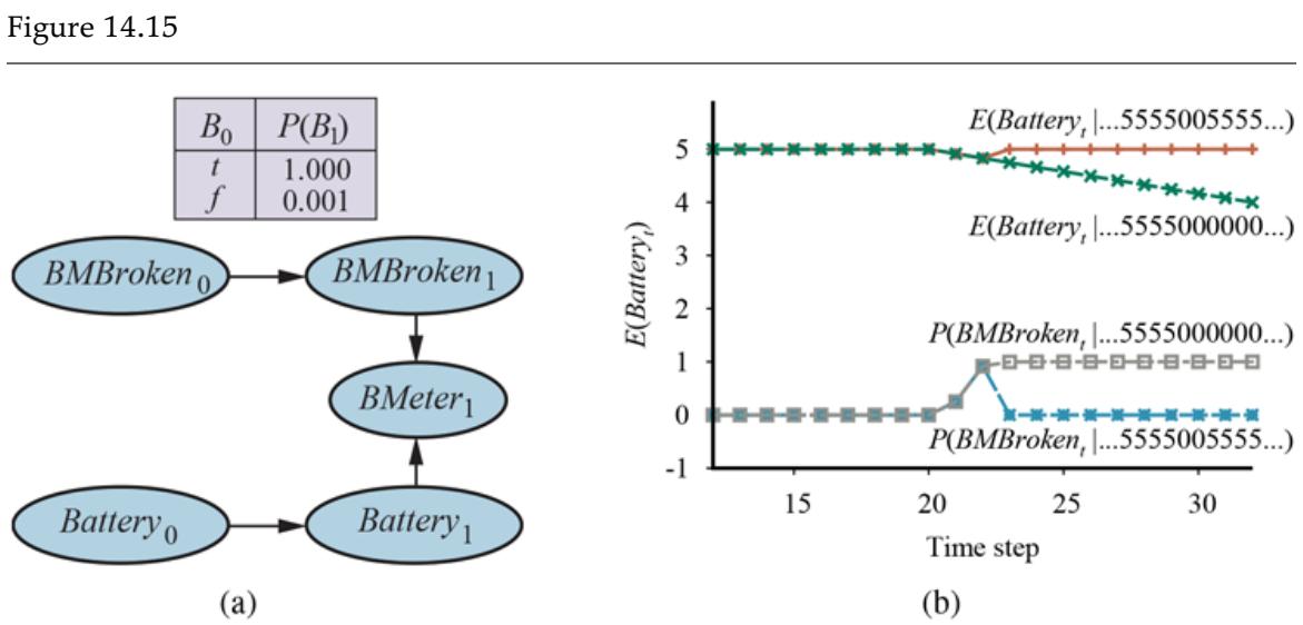
1. A DBN fragment showing the sensor status variable required for modeling persistent failure of the battery sensor. (b) Upper curves: trajectories of the expected value of for the “transient failure” and “permanent failure” observations sequences. Lower curves: probability trajectories for given the two observation sequences.

So far, we have merely scratched the surface of the problem of representing complex processes. The variety of transition models is huge, encompassing topics as disparate as modeling the human endocrine system and modeling multiple vehicles driving on a freeway. Sensor modeling is also a vast subfield in itself. But dynamic Bayesian networks can model even subtle phenomena, such as sensor drift, sudden decalibration, and the effects of exogenous conditions (such as weather) on sensor readings.

14.5.2 Exact inference in DBNs

Having sketched some ideas for representing complex processes as DBNs, we now turn to the question of inference. In a sense, this question has already been answered: dynamic Bayesian networks are Bayesian networks, and we already have algorithms for inference in Bayesian networks. Given a sequence of observations, one can construct the full Bayesian network representation of a DBN by replicating slices until the network is large enough to accommodate the observations, as in Figure 14.16 . This technique is called unrolling. (Technically, the DBN is equivalent to the semi-infinite network obtained by unrolling forever. Slices added beyond the last observation have no effect on inferences within the observation period and can be omitted.) Once the DBN is unrolled, one can use any of the inference algorithms—variable elimination, clustering methods, and so on—described in Chapter 13 .

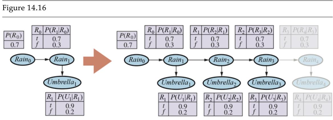
Unfortunately, a naive application of unrolling would not be particularly efficient. If we want to perform filtering or smoothing with a long sequence of observations , the unrolled network would require space and would thus grow without bound as more observations were added. Moreover, if we simply run the inference algorithm anew each time an observation is added, the inference time per update will also increase as .

Looking back to Section 14.2.1 , we see that constant time and space per filtering update can be achieved if the computation can be done recursively. Essentially, the filtering update in Equation (14.5) works by summing out the state variables of the previous time step to get the distribution for the new time step. Summing out variables is exactly what the variable elimination (Figure 13.13 ) algorithm does, and it turns out that running variable

elimination with the variables in temporal order exactly mimics the operation of the recursive filtering update in Equation (14.5) . The modified algorithm keeps at most two slices in memory at any one time: starting with slice 0, we add slice 1, then sum out slice 0, then add slice 2, then sum out slice 1, and so on. In this way, we can achieve constant space and time per filtering update. (The same performance can be achieved by suitable modifications to the clustering algorithm.) Exercise 14.DBNE asks you to verify this fact for the umbrella network.

So much for the good news; now for the bad news: It turns out that the “constant” for the per-update time and space complexity is, in almost all cases, exponential in the number of state variables. What happens is that, as the variable elimination proceeds, the factors grow to include all the state variables (or, more precisely, all those state variables that have parents in the previous time slice). The maximum factor size is and the total update cost per step is , where is the domain size of the variables and is the maximum number of parents of any state variable.

Of course, this is much less than the cost of HMM updating, which is , but it is still infeasible for large numbers of variables. This grim fact means is that even though we can use DBNs to represent very complex temporal processes with many sparsely connected variables, we cannot reason efficiently and exactly about those processes.

The DBN model itself, which represents the prior joint distribution over all the variables, is factorable into its constituent CPTs, but the posterior joint distribution conditioned on an observation sequence—that is, the forward message—is generally not factorable. The problem is intractable in general, so we must fall back on approximate methods.

14.5.3 Approximate inference in DBNs

Section 13.4 described two approximation algorithms: likelihood weighting (Figure 13.18 ) and Markov chain Monte Carlo (MCMC, Figure 13.20 ). Of the two, the former is most easily adapted to the DBN context. (An MCMC filtering algorithm is described briefly in the notes at the end of this chapter.) We will see, however, that several improvements are required over the standard likelihood weighting algorithm before a practical method emerges.

Recall that likelihood weighting works by sampling the nonevidence nodes of the network in topological order, weighting each sample by the likelihood it accords to the observed evidence variables. As with the exact algorithms, we could apply likelihood weighting directly to an unrolled DBN, but this would suffer from the same problems of increasing time and space requirements per update as the observation sequence grows. The problem is that the standard algorithm runs each sample in turn, all the way through the network.

Instead, we can simply run all samples together through the DBN, one slice at a time. The modified algorithm fits the general pattern of filtering algorithms, with the set of samples as the forward message. The first key innovation, then, is to use the samples themselves as an approximate representation of the current state distribution. This meets the requirement of a “constant” time per update, although the constant depends on the number of samples required to maintain an accurate approximation. There is also no need to unroll the DBN, because we need to have in memory only the current slice and the next slice. This approach is called sequential importance sampling or SIS.

Sequential importance sampling

In our discussion of likelihood weighting in Chapter 13 , we pointed out that the algorithm’s accuracy suffers if the evidence variables are “downstream” from the variables being sampled, because in that case the samples are generated without any influence from the evidence and will nearly all have very low weights.

Now if we look at the typical structure of a DBN—say, the umbrella DBN in Figure 14.16 we see that indeed the early state variables will be sampled without the benefit of the later evidence. In fact, looking more carefully, we see that none of the state variables have any evidence variables among its ancestors! Hence, although the weight of each sample will depend on the evidence, the actual set of samples generated will be completely independent of the evidence. For example, even if the boss brings in the umbrella every day, the sampling process could still hallucinate endless days of sunshine.

What this means in practice is that the fraction of samples that remain reasonably close to the actual series of events (and therefore have non-negligible weights) drops exponentially with , the length of the sequence. In other words, to maintain a given level of accuracy, we need to increase the number of samples exponentially with . Given that a real-time filtering algorithm can use only a bounded number of samples, what happens in practice is that the error blows up after a very small number of update steps. Figure 14.19 on 494 shows this effect for SIS applied to the grid-world localization problem from Section 14.3 : even with 100,000 samples, the SIS approximation fails completely after about 20 steps.

Clearly, we need a better solution. The second key innovation is to focus the set of samples on the high-probability regions of the state space. This can be done by throwing away samples that have very low weight, according to the observations, while replicating those that have high weight. In that way, the population of samples will stay reasonably close to reality. If we think of samples as a resource for modeling the posterior distribution, then it makes sense to use more samples in regions of the state space where the posterior is higher.

A family of algorithms called particle filtering is designed to do just that. (Another early name was sequential importance sampling with resampling, but for some reason it failed on catch on.) Particle filtering works as follows: First, we generate a population of samples from the prior distribution . Then the update cycle is repeated for each time step:

• 1. Each sample is propagated forward by sampling the next state value given the current value for the sample, based on the transition model .
• 2. Each sample is weighted by the likelihood it assigns to the new evidence, .
• 3. The population is resampled to generate a new population of samples. Each new sample is selected from the current population; the probability that a particular sample is selected is proportional to its weight. The new samples are unweighted.

The algorithm is shown in detail in Figure 14.17 , and its operation for the umbrella DBN is illustrated in Figure 14.18 .

The particle filtering algorithm implemented as a recursive update operation with state (the set of samples). Each of the sampling operations involves sampling the relevant slice variables in topological order, much as in PRIOR-SAMPLE. The WEIGHTED-SAMPLE-WITH-REPLACEMENT operation can be implemented to run in expected time. The step numbers refer to the description in the text.

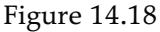
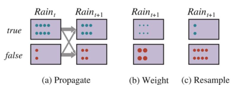
The particle filtering update cycle for the umbrella DBN with , showing the sample populations of each state. (a) At time , 8 samples indicate and 2 indicate . Each is propagated forward by sampling the next state through the transition model. At time , 6 samples indicate and 4 indicate . (b) is observed at . Each sample is weighted by its likelihood for the observation, as indicated by the size of the circles. (c) A new set of 10 samples is generated by weighted random selection from the current set, resulting in 2 samples that indicate and 8 that indicate .

We can show that this algorithm is consistent—gives the correct probabilities as tends to infinity—by examining the operations in one update cycle. We assume that the sample population starts with a correct representation of the forward message—that is, at time . Writing for the number of samples occupying state after observations have been processed, we therefore have

(14.23)

\[N(\mathbf{x}\_t|\mathbf{e}\_{1:t})/N = P(\mathbf{x}\_t|\mathbf{e}\_{1:t})\]

for large . Now we propagate each sample forward by sampling the state variables at , given the values for the sample at . The number of samples reaching state from each is the transition probability times the population of ; hence, the total number of samples reaching is

\[N(\mathbf{x}\_{t+1}|\mathbf{e}\_{1:t}) = \sum\_{\mathbf{x}\_t} P(\mathbf{x}\_{t+1}|\mathbf{x}\_t) N(\mathbf{x}\_t|\mathbf{e}\_{1:t}).\]

Now we weight each sample by its likelihood for the evidence at . A sample in state receives weight . The total weight of the samples in after seeing is therefore

\[W(\mathbf{x}\_{t+1}|\mathbf{e}\_{1:t+1}) = P(\mathbf{e}\_{t+1}|\mathbf{x}\_{t+1})N(\mathbf{x}\_{t+1}|\mathbf{e}\_{1:t})\dots\]

Now for the resampling step. Since each sample is replicated with probability proportional to its weight, the number of samples in state after resampling is proportional to the total weight in before resampling:

\[\begin{split} N(\mathbf{x}\_{t+1}|\mathbf{e}\_{1:t+1})/N &= \alpha W(\mathbf{x}\_{t+1}|\mathbf{e}\_{1:t+1}) \\ &= \alpha P(\mathbf{e}\_{t+1}|\mathbf{x}\_{t+1}) N(\mathbf{x}\_{t+1}|\mathbf{e}\_{1:t}) \\ &= \alpha P(\mathbf{e}\_{t+1}|\mathbf{x}\_{t+1}) \sum\_{\mathbf{x}\_t} P(\mathbf{x}\_{t+1}|\mathbf{x}\_t) N(\mathbf{x}\_t|\mathbf{e}\_{1:t}) \\ &= \alpha NP(\mathbf{e}\_{t+1}|\mathbf{x}\_{t+1}) \sum\_{\mathbf{x}\_t} P(\mathbf{x}\_{t+1}|\mathbf{x}\_t) P(\mathbf{x}\_t|\mathbf{e}\_{1:t}) \quad \text{(by 14.23)} \\ &= \alpha' P(\mathbf{e}\_{t+1}|\mathbf{x}\_{t+1}) \sum\_{\mathbf{x}\_t} P(\mathbf{x}\_{t+1}|\mathbf{x}\_t) P(\mathbf{x}\_t|\mathbf{e}\_{1:t}) \\ &= P(\mathbf{x}\_{t+1}|\mathbf{e}\_{1:t+1}) \quad \text{(by 14.5)}. \end{split}\]

Therefore the sample population after one update cycle correctly represents the forward message at time .

Particle filtering is consistent, therefore, but is it efficient? For many practical cases, it seems that the answer is yes: particle filtering seems to maintain a good approximation to the true posterior using a constant number of samples. Figure 14.19 shows that particle filtering does a good job on the grid-world localization problem with only a thousand samples. It also works on real-world problems: the algorithm supports thousands of applications in science and engineering. (Some references are given at the end of the chapter.) It handles combinations of discrete and continuous variables as well as nonlinear and non-Gaussian

models for continuous variables. Under certain assumptions—in particular, that the probabilities in the transition and sensor models are bounded away from 0 and 1—it is also possible to prove that the approximation maintains bounded error with high probability, as the figure suggests.

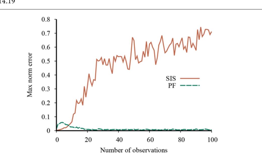
Figure 14.19

Max norm error in the grid-world location estimate (compared to exact inference) for likelihood weighting (sequential importance sampling) with 100,000 samples and particle filtering with 1,000 samples; data averaged over 50 runs.

The particle filtering algorithm does have weaknesses, however. Let’s see how it performs for the vacuum world with dirt added. Recall from Section 14.3.2 that this increases the state space size by a factor of , making exact HMM inference infeasible. We want the robot to wander around and build a map of where the dirt is located. (This is a simple example of simultaneous localization and mapping or SLAM, which we cover in more depth in Chapter 26 .) Let mean that square is dirty at time and let be true if and only if the robot detects dirt at time . We’ll assume that, in any given square, dirt persists with probability , whereas a clean square becomes dirty with probability (which means that each square is dirty half the time, on average). The robot has a dirt sensor for its current location; the sensor is accurate with probability 0.9. Figure 14.20 shows the DBN.

Figure 14.20

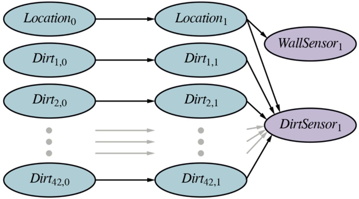
A dynamic Bayes net for simultaneous localization and mapping in the stochastic-dirt vacuum world. Dirty squares persist with probability , and clean squares become dirty with probability . The local dirt sensor is 90% accurate, for the square in which the robot is currently located.

For simplicity, we’ll start by assuming that the robot has a perfect location sensor, rather than the noisy wall sensor. The algorithm’s performance is shown in Figure 14.21(a) , where its estimates for dirt are compared to the results of exact inference. (We’ll see shortly how exact inference is possible.) For low values of the dirt persistence , the error remains small—but this is no great achievement, because for every square the true posterior for dirt is close to 0.5 if the robot hasn’t visited that square recently. For higher values of , the dirt stays around longer, so visiting a square yields more useful information that is valid over a longer period. Perhaps surprisingly, particle filtering does worse for higher values of . It fails completely when , even though that seems like the easiest case: the dirt arrives at time 0 and stays put forever, so after a few tours of the world, the robot should have a closeto-perfect dirt map. Why does particle filtering fail in this case?

Figure 14.21

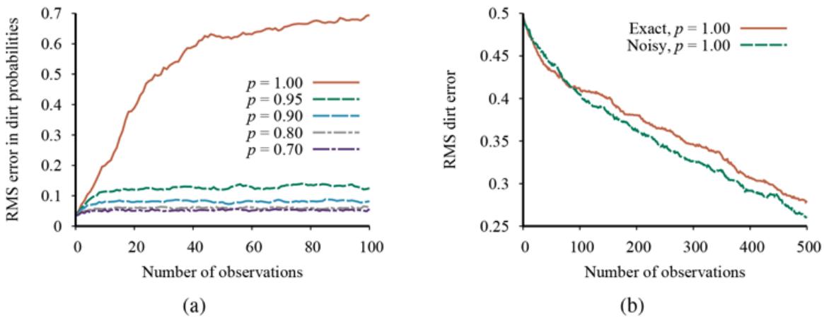
1. Performance of the standard particle filtering algorithm with 1,000 particles, showing RMS error in marginal dirt probabilities compared to exact inference for different values of the dirt persistence . (b) Performance of Rao-Blackwellized particle filtering (100 particles) compared to ground truth, for both exact location sensing and noisy wall sensing and with deterministic dirt. Data averaged over 20 runs.

It turns out that the theoretical condition requiring that “the probabilities in the transition and sensor models are strictly greater than 0 and less than 1” is more than mere mathematical pedantry. What happens is first each particle initially contains 42 guesses from about which squares have dirt and which do not. Then, the state for each particle is projected forward in time according to the transition model. Unfortunately, the transition model for deterministic dirt is deterministic: the dirt stays exactly where it is. Thus, the initial guesses in each particle are never updated by the evidence.

The chance that the initial guesses are all correct is or about , so it is vanishingly unlikely that a thousand particles (or even a million particles) will include one with the correct dirt map. Typically, the best particle out of a thousand will get about 32 right and 10 wrong, and usually there will be only one such particle, or perhaps a handful. One of those best particles will come to dominate the total likelihood as time progresses and the diversity of the population of particles will collapse. Then, because all the particles agree on a single, incorrect map, the algorithm becomes convinced that that map is correct and never changes its mind.

Fortunately, the problem of simultaneous localization and mapping has a special structure: conditioned on the sequence of robot locations, the dirt statuses of the individual squares are independent (Exercise 14.RBPF). More specifically,

This means it is useful to apply a statistical trick called Rao-Blackwellization, which is based on the simple idea that exact inference is always more accurate than sampling, even if it’s only for a subset of the variables. (See Exercise 14.RAOB.) For the SLAM problem, we run particle filtering on the robot location and then, for each particle, we run exact HMM inference for each dirt square independently, conditioned on the location sequence in that particle. Each particle therefore contains a sampled location plus 42 exact marginal posteriors for the 42 squares—exact, that is, assuming that the hypothesized location trajectory followed by that particle is correct. This approach, called the Rao-Blackwellized particle filter, handles the case of deterministic dirt with no difficulty, gradually building an exact dirt map with either exact location sensing or noisy wall sensing, as shown in Figure 14.21(b) .

Rao-Blackwellization

In cases that do not satisfy the kind of conditional independence structure exemplified by Equation (14.24) , Rao-Blackwellization is not applicable. The notes at the end of the chapter mention a number of algorithms that have been proposed to handle the general problem of filtering with static variables. None has the elegance and broad applicability of the particle filter, but several are effective in practice on certain classes of problems.

Rao-Blackwellized particle filter

Summary

This chapter has addressed the general problem of representing and reasoning about probabilistic temporal processes. The main points are as follows:

• The changing state of the world is handled by using a set of random variables to represent the state at each point in time.
• Representations can be designed to (roughly) satisfy the Markov property, so that the future is independent of the past given the present. Combined with the assumption that the process is time-homogeneous, this greatly simplifies the representation.
• A temporal probability model can be thought of as containing a transition model describing the state evolution and a sensor model describing the observation process.
• The principal inference tasks in temporal models are filtering (state estimation), prediction, smoothing, and computing the most likely explanation. Each of these tasks can be achieved using simple, recursive algorithms whose run time is linear in the length of the sequence.
• Three families of temporal models were studied in more depth: hidden Markov models, Kalman filters, and dynamic Bayesian networks (which include the other two as special cases).
• Unless special assumptions are made, as in Kalman filters, exact inference with many state variables is intractable. In practice, the particle filtering algorithm and its descendants are an effective family of approximation algorithms.

Bibliographical and Historical Notes

Many of the basic ideas for estimating the state of dynamical systems came from the mathematician C. F. Gauss 1809, who formulated a deterministic least-squares algorithm for the problem of estimating orbits from astronomical observations. A. A. Markov (1913) developed what was later called the Markov assumption in his analysis of stochastic processes; he estimated a first-order Markov chain on letters from the text of Eugene Onegin. The general theory of Markov chains and their mixing times is covered by Levin et al. (2008).

Significant classified work on filtering was done during World War II by Wiener (1942) for continuous-time processes and by Kolmogorov (1941) for discrete-time processes. Although this work led to important technological developments over the next 20 years, its use of a frequency-domain representation made many calculations quite cumbersome. Direct statespace modeling of the stochastic process turned out to be simpler, as shown by Peter Swerling (1959) and Rudolf Kalman (1960). The latter paper described what is now known as the Kalman filter for forward inference in linear systems with Gaussian noise; Kalman’s results had, however, been obtained previously by the Danish astronomer Thorvold Thiele (1880) and by the Russian physicist Ruslan Stratonovich (1959). After a visit to NASA Ames Research Center in 1960, Kalman saw the applicability of the method to the tracking of rocket trajectories, and the filter was later implemented for the Apollo missions.

Key results on smoothing were derived by Rauch et al. (1965), and the impressively named Rauch–Tung–Striebel smoother is still a standard technique today. Many early results are gathered in Gelb (1974). Bar-Shalom and Fortmann (1988) give a more modern treatment with a Bayesian flavor, as well as many references to the vast literature on the subject. Chatfield (1989) and Box et al., (2016) cover the control theory approach to time series analysis.

The hidden Markov model and associated algorithms for inference and learning, including the forward–backward algorithm, were developed by Baum and Petrie (1966). The Viterbi algorithm first appeared in (Viterbi, 1967). Similar ideas also appeared independently in the Kalman filtering community (Rauch et al., 1965).

The forward–backward algorithm was one of the main precursors of the general formulation of the EM algorithm (Dempster et al., 1977); see also Chapter 20 . Constant-space smoothing appears in Binder et al. (1997b), as does the divide-and-conquer algorithm developed in Exercise 14.ISLE. Constant-time fixed-lag smoothing for HMMs first appeared in Russell and Norvig (2003).

HMMs have found many applications in language processing (Charniak, 1993), speech recognition (Rabiner and Juang, 1993), machine translation (Och and Ney, 2003), computational biology (Krogh et al., 1994; Baldi et al., 1994), financial economics (Bhar and Hamori, 2004) and other fields. There have been several extensions to the basic HMM model: for example, the Hierarchical HMM (Fine et al., 1998) and Layered HMM (Oliver et al., 2004) introduce structure back into the model, replacing the single state variable of HMMs.

Dynamic Bayesian networks (DBNs) can be viewed as a sparse encoding of a Markov process and were first used in AI by Dean and Kanazawa (1989b), Nicholson and Brady (1992), and Kjaerulff (1992). The last work extends the HUGIN Bayes net system to accommodate dynamic Bayesian networks. The book by Dean and Wellman (1991) helped popularize DBNs and the probabilistic approach to planning and control within AI. Murphy (2002) provides a thorough analysis of DBNs.

Dynamic Bayesian networks have become popular for modeling a variety of complex motion processes in computer vision (Huang et al., 1994; Intille and Bobick, 1999), (Huang et al., 1994; Intille and Bobick, 1999). Like HMMs, they have found applications in speech recognition (Zweig and Russell, 1998; Livescu et al., 2003), robot localization (Theocharous et al., 2004), and genomics (Murphy and Mian, 1999; Li et al., 2011). Other application areas include gesture analysis (Suk et al., 2010), driver fatigue detection (Yang et al., 2010), and urban traffic modeling (Hofleitner et al., 2012).

The link between HMMs and DBNs, and between the forward–backward algorithm and Bayesian network propagation, was explicated by Smyth et al., (1997). A further unification with Kalman filters (and other statistical models) appears in Roweis and Ghahramani (1999). Procedures exist for learning the parameters (Binder et al., 1997a; Ghahramani, 1998) and structures (Friedman et al., 1998) of DBNs. Continuous-time Bayesian networks (Nodelman et al., 2002) are the discrete-state, continuous-time analog of DBNs, avoiding the need to choose a particular duration for time steps.

The first sampling algorithms for filtering (also called sequential Monte Carlo methods) were developed in the control theory community by Handschin and Mayne (1969), and the resampling idea that is the core of particle filtering appeared in a Russian control journal (Zaritskii et al., 1975). It was later reinvented in statistics as sequential importance sampling with resampling, or SIR (Rubin, 1988; Liu and Chen, 1998), in control theory as particle filtering (Gordon et al., 1993; Gordon, 1994), in AI as survival of the fittest (Kanazawa et al., 1995), and in computer vision as condensation (Isard and Blake, 1996).

Evidence reversal

The paper by Kanazawa et al. (1995) includes an improvement called evidence reversal whereby the state at time is sampled conditional on both the state at time and the evidence at time . This allows the evidence to influence sample generation directly and was proved by Doucet (1997) and Liu and Chen (1998) to reduce the approximation error.

Particle filtering has been applied in many areas, including tracking complex motion patterns in video (Isard and Blake, 1996), predicting the stock market (de Freitas et al., 2000), and diagnosing faults on planetary rovers (Verma et al., 2004). Since its invention, tens of thousands of papers have been published on applications and variants of the algorithm. Scalable implementations on parallel hardware have become important; although one might think it straightforward to distribute particles across up to processor threads, the basic algorithm requires synchronized communication among threads for the resampling step (Hendeby et al., 2010). The particle cascade algorithm (Paige et al., 2014) removes the synchronization requirement, resulting in much faster parallel computation.

The Rao-Blackwellized particle filter is due to Doucet et al., (2000) and Murphy and Russell (2001); its application to practical localization and mapping problems in robotics is described in Chapter 26 . Many other algorithms have been proposed to handle more general filtering problems with static or nearly-static variables, including the resample–

move algorithm (Gilks and Berzuini, 2001), the Liu–West algorithm (Liu and West, 2001), the Storvik filter (Storvik, 2002), the extended parameter filter (Erol et al., 2013), and the assumed parameter filter (Erol et al., 2017). The latter is a hybrid of particle filtering with a much older idea called assumed-density filter. An assumed-density filter assumes that the posterior distribution over states at time belongs to a particular finitely parameterized family; if the projection and update steps take it outside this family, the distribution is projected back to give the best approximation within the family. For DBNs, the Boyen– Koller algorithm (Boyen et al., 1999) and the factored frontier algorithm (Murphy and Weiss, 2001) assume that the posterior distribution can be approximated well by a product of small factors.

Assumed-density filter

Factored frontier

MCMC methods (see Section 13.4.2 ) can be applied to the filtering problem; for example, Gibbs sampling can be applied directly to an unrolled DBN. The particle MCMC family of algorithms (Andrieu et al., 2010; Lindsten et al., 2014) combines MCMC on the unrolled temporal model with particle filtering to generate the MCMC proposals; although it provably converges to the correct posterior distribution in the general case (i.e., with both static and dynamic variables), it is an offline algorithm. To avoid the problem of increasing update times as the unrolled network grows, the decayed MCMC filter (Marthi et al., 2002) prefers to sample more recent state variables, with a probability that decreases for variables further in the past.

Particle MCMC

Decayed MCMC

The book by Doucet et al. (2001) collects many important papers on sequential Monte Carlo (SMC) algorithms, of which particle filtering is the most important instance. There are useful tutorials by Arulampalam et al. (2002) and Doucet and Johansen (2011). There are also several theoretical results concerning conditions under which SMC methods retain a bounded error indefinitely compared to the true posterior (Crisan and Doucet, 2002; Del Moral, 2004; Del Moral et al., 2006).

Chapter 15 Probabilistic Programming

In which we explain the idea of universal languages for probabilistic knowledge representation and inference in uncertain domains.

The spectrum of representations—atomic, factored, and structured—has been a persistent theme in AI. For deterministic models, search algorithms assume only an atomic representation; CSPs and propositional logic provide factored representations; and firstorder logic and planning systems take advantage of structured representations. The expressive power afforded by structured representations yields models that are vastly more concise than the equivalent factored or atomic descriptions.

For probabilistic models, Bayesian networks as described in Chapters 13 and 14 are factored representations: the set of random variables is fixed and finite, and each has a fixed range of possible values. This fact limits the applicability of Bayesian networks, because the Bayesian network representation for a complex domain is simply too large. This makes it infeasible to construct such representations by hand and infeasible to learn them from any reasonable amount of data.

The problem of creating an expressive formal language for probabilistic information has taxed some of the greatest minds in history, including Gottfried Leibniz (the co-inventor of calculus), Jacob Bernoulli (discoverer of , the calculus of variations, and the Law of Large Numbers), Augustus De Morgan, George Boole, Charles Sanders Peirce (one of the principal logicians of the 19th century), John Maynard Keynes (the leading economist of the 20th century), and Rudolf Carnap (one of the greatest analytical philosophers of the 20th century). The problem resisted these and many other efforts until the 1990s.

Thanks in part to the development of Bayesian networks, there are now mathematically elegant and eminently practical formal languages that allow the creation of probabilistic models for very complex domains. These languages are universal in the same sense that Turing machines are universal: they can represent any computable probability model, just as Turing machines can represent any computable function. In addition, these languages come with general-purpose inference algorithms, roughly analogous to sound and complete logical inference algorithms such as resolution.

There are two routes to introducing expressive power into probability theory. The first is via logic: to devise a language that defines probabilities over first-order possible worlds, rather than the propositional possible worlds of Bayes nets. This route is covered in Sections 15.1 and 15.2 , with Section 15.3 covering the specific case of temporal reasoning. The second route is via traditional programming languages: we introduce stochastic elements—random choices, for example—into such languages, and view programs as defining probability distributions over their own execution traces. This approach is covered in Section 15.4 .

Both routes lead to a probabilistic programming language (PPL). The first route leads to declarative PPLs, which bear roughly the same relationship to general PPLs as logic programming (Chapter 9 ) does to general programming languages.

Probabilistic programming language (PPL)

15.1 Relational Probability Models

Recall from Chapter 12 that a probability model defines a set of possible worlds with a probability for each world . For Bayesian networks, the possible worlds are assignments of values to variables; for the Boolean case in particular, the possible worlds are identical to those of propositional logic.

For a first-order probability model, then, it seems we need the possible worlds to be those of first-order logic—that is, a set of objects with relations among them and an interpretation that maps constant symbols to objects, predicate symbols to relations, and function symbols to functions on those objects. (See Section 8.2 .) The model also needs to define a probability for each such possible world, just as a Bayesian network defines a probability for each assignment of values to variables.

Let us suppose, for a moment, that we have figured out how to do this. Then, as usual (see page 389), we can obtain the probability of any first-order logical sentence (phi) as a sum over the possible worlds where it is true:

(15.1)

\[P(\phi) = \sum\_{\omega:\phi \text{ is true in } \omega} P(\omega).\]

Conditional probabilities can be obtained similarly, so we can, in principle, ask any question we want of our model—and get an answer. So far, so good.

There is, however, a problem: the set of first-order models is infinite. We saw this explicitly in Figure 8.4 on page 259, which we show again in Figure 15.1 (top). This means that (1) the summation in Equation (15.1) could be infeasible, and (2) specifying a complete, consistent distribution over an infinite set of worlds could be very difficult.

Figure 15.1

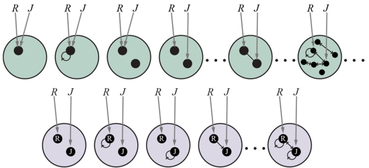
Top: Some members of the set of all possible worlds for a language with two constant symbols, and , and one binary relation symbol, under the standard semantics for first-order logic. Bottom: the possible worlds under database semantics. The interpretation of the constant symbols is fixed, and there is a distinct object for each constant symbol.

In this section, we avoid this issue by considering the database semantics defined in Section 8.2.8 (page 264). The database semantics makes the unique names assumption—here, we adopt it for the constant symbols. It also assumes domain closure—there are no more objects beyond those that are named. We can then guarantee a finite set of possible worlds by making the set of objects in each world be exactly the set of constant symbols that are used; as shown in Figure 15.1 (bottom), there is no uncertainty about the mapping from symbols to objects or about the objects that exist.

We will call models defined in this way relational probability models, or RPMs. The most significant difference between the semantics of RPMs and the database semantics introduced in Section 8.2.8 is that RPMs do not make the closed-world assumption—in a probabilistic reasoning system we can’t just assume that every unknown fact is false. 1

1 The name relational probability model was given by Pfeffer, (2000) to a slightly different representation, but the underlying ideas are the same.

Relational probability model

15.1.1 Syntax and semantics

Let us begin with a simple example: suppose that an online book retailer would like to provide overall evaluations of products based on recommendations received from its customers. The evaluation will take the form of a posterior distribution over the quality of the book, given the available evidence. The simplest solution is to base the evaluation on the average recommendation, perhaps with a variance determined by the number of recommendations, but this fails to take into account the fact that some customers are kinder than others and some are less honest than others. Kind customers tend to give high recommendations even to fairly mediocre books, while dishonest customers give very high or very low recommendations for reasons other than quality—they might be paid to promote some publisher’s books. 2

2 A game theorist would advise a dishonest customer to avoid detection by occasionally recommending a good book from a competitor. See Chapter 18 .

For a single customer recommending a single book , the Bayes net might look like the one shown in Figure 15.2(a) . (Just as in Section 9.1 , expressions with parentheses such as are just fancy symbols—in this case, fancy names for random variables.) With two customers and two books, the Bayes net looks like the one in Figure 15.2(b) . For larger numbers of books and customers, it is quite impractical to specify a Bayes net by hand.

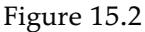
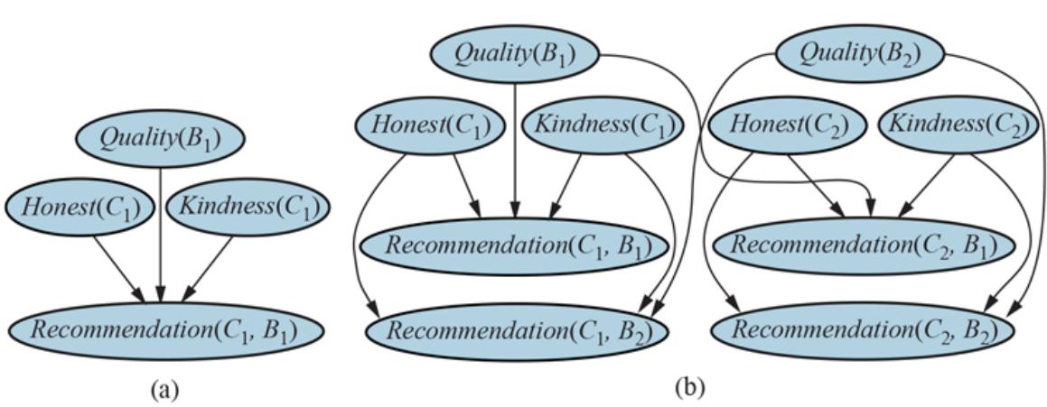
1. Bayes net for a single customer recommending a single book . is Boolean, while the other variables have integer values from 1 to 5. (b) Bayes net with two customers and two books.

Fortunately, the network has a lot of repeated structure. Each variable has as its parents the variables , , and . Moreover, the conditional probability tables (CPTs) for all the variables are identical, as are those for all the variables, and so on. The situation seems tailormade for a first-order language. We would like to say something like

\[Recommensulation (c, b) \sim RecCPT(Homest \langle c \rangle, Kindness \langle c \rangle, Quality(b))\]

which means that a customer’s recommendation for a book depends probabilistically on the customer’s honesty and kindness and the book’s quality according to a fixed CPT.

Like first-order logic, RPMs have constant, function, and predicate symbols. We will also assume a type signature for each function—that is, a specification of the type of each argument and the function’s value. (If the type of each object is known, many spurious possible worlds are eliminated by this mechanism; for example, we need not worry about the kindness of each book, books recommending customers, and so on.) For the bookrecommendation domain, the types are and , and the type signatures for the functions and predicates are as follows:

Type signature

The constant symbols will be whatever customer and book names appear in the retailer’s data set. In the example given in Figure 15.2(b) , these were and .

Given the constants and their types, together with the functions and their type signatures, the basic random variables of the RPM are obtained by instantiating each function with each possible combination of objects. For the book recommendation model, the basic random variables include , , , and so on.

These are exactly the variables appearing in Figure 15.2(b) . Because each type has only finitely many instances (thanks to the domain closure assumption), the number of basic random variables is also finite.

Basic random variable

To complete the RPM, we have to write the dependencies that govern these random variables. There is one dependency statement for each function, where each argument of the function is a logical variable (i.e., a variable that ranges over objects, as in first-order logic). For example, the following dependency states that, for every customer , the prior probability of honesty is 0.99 true and 0.01 false:

\[Honest(c) \sim \langle 0.99, 0.01 \rangle\]

Similarly, we can state prior probabilities for the kindness value of each customer and the quality of each book, each on the 1–5 scale:

Finally, we need the dependency for recommendations: for any customer and book , the score depends on the honesty and kindness of the customer and the quality of the book:

where is a separately defined conditional probability table with rows, each with 5 entries. For the purposes of illustration, we’ll assume that an honest recommendation for a book of quality from a person of kindness is uniformly distributed in the range .

The semantics of the RPM can be obtained by instantiating these dependencies for all known constants, giving a Bayesian network (as in Figure 15.2(b) ) that defines a joint distribution over the RPM’s random variables.3

3 Some technical conditions are required for an RPM to define a proper distribution. First, the dependencies must be acyclic; otherwise the resulting Bayesian network will have cycles. Second, the dependencies must (usually) be well-founded: there can be no infinite ancestor chains, such as might arise from recursive dependencies. See Exercise 15.HAMD for an exception to this rule.

The set of possible worlds is the Cartesian product of the ranges of all the basic random variables, and, as with Bayesian networks, the probability for each possible world is the product of the relevant conditional probabilities from the model. With customers and books, there are variables, variables, variables, and variables, leading to possible worlds. With ten million books and a billion customers, that’s about worlds. Thanks to the expressive power of RPMs, the complete probability model still has only fewer than 300 parameters—most of them in the table.

We can refine the model by asserting a context-specific independence (see page 420) to reflect the fact that dishonest customers ignore quality when giving a recommendation; moreover, kindness plays no role in their decisions. Thus, is independent of and when :

This kind of dependency may look like an ordinary if–then–else statement in a programming language, but there is a key difference: the inference engine doesn’t necessarily know the value of the conditional test because is a random variable.

We can elaborate this model in endless ways to make it more realistic. For example, suppose that an honest customer who is a fan of a book’s author always gives the book a 5, regardless of quality:

Again, the conditional test is unknown, but if a customer gives only 5s to a particular author’s books and is not otherwise especially kind, then the posterior probability that the customer is a fan of that author will be high. Furthermore, the posterior

distribution will tend to discount the customer’s 5s in evaluating the quality of that author’s books.

In this example, we implicitly assumed that the value of is known for every , but this may not be the case. How can the system reason about whether, say, is a fan of when is unknown? The answer is that the system may have to reason about all possible authors. Suppose (to keep things simple) that there are just two authors, and . Then is a random variable with two possible values, and , and it is a parent of . The variables and are parents too. The conditional distribution for is then essentially a multiplexer in which the parent acts as a selector to choose which of and actually gets to influence the recommendation. A fragment of the equivalent Bayes net is shown in Figure 15.3 . Uncertainty in the value of , which affects the dependency structure of the network, is an instance of relational uncertainty.

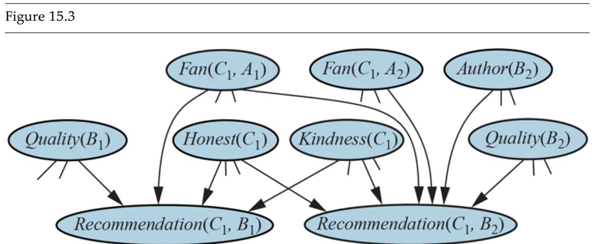
Fragment of the equivalent Bayes net for the book recommendation RPM when is unknown.

Multiplexer

Relational uncertainty

In case you are wondering how the system can possibly work out who the author of is: consider the possibility that three other customers are fans of (and have no other favorite authors in common) and all three have given a 5, even though most other customers find it quite dismal. In that case, it is extremely likely that is the author of . The emergence of sophisticated reasoning like this from an RPM model of just a few lines is an intriguing example of how probabilistic influences spread through the web of interconnections among objects in the model. As more dependencies and more objects are added, the picture conveyed by the posterior distribution often becomes clearer and clearer.

15.1.2 Example: Rating player skill levels

Many competitive games have a numerical measure of players’ skill levels, sometimes called a rating. Perhaps the best-known is the Elo rating for chess players, which rates a typical beginner at around 800 and the world champion usually somewhere above 2800. Although Elo ratings have a statistical basis, they have some ad hoc elements. We can develop a Bayesian rating scheme as follows: each player has an underlying skill level ; in each game , ’s actual performance is , which may vary from the underlying skill level; and the winner of is the player whose performance in is better. As an RPM, the model looks like this:

Rating

where is the variance of a player’s actual performance in any specific game relative to the player’s underlying skill level. Given a set of players and games, as well as outcomes for some of the games, an RPM inference engine can compute a posterior distribution over the skill of each player and the probable outcome of any additional game that might be played.

For team games, we’ll assume, as a first approximation, that the overall performance of team in game is the sum of the individual performances of the players on :

Even though the individual performances are not visible to the ratings engine, the players’ skill levels can still be estimated from the results of several games, as long as the team compositions vary across games. Microsoft’s ratings engine uses this model, along with an efficient approximate inference algorithm, to serve hundreds of millions of users every day.

This model can be elaborated in numerous ways. For example, we might assume that weaker players have higher variance in their performance; we might include the player’s role on the team; and we might consider specific kinds of performance and skill—e.g., defending and attacking—in order to improve team composition and predictive accuracy.

15.1.3 Inference in relational probability models

The most straightforward approach to inference in RPMs is simply to construct the equivalent Bayesian network, given the known constant symbols belonging to each type. With books and customers, the basic model given previously could be constructed with simple loops: 4

4 Several statistical packages would view this code as defining the RPM, rather than just constructing a Bayes net to perform inference in the RPM. This view, however, misses an important role for RPM syntax: without a syntax with clear semantics, there is no way the model structure can be learned from data.

This technique is called grounding or unrolling; it is the exact analog of propositionalization for first-order logic (page 280). The obvious drawback is that the resulting Bayes net may be very large. Furthermore, if there are many candidate objects for an unknown relation or function—for example, the unknown author of —then some variables in the network may have many parents.

Grounding

Unrolling

Fortunately, it is often possible to avoid generating the entire implicit Bayes net. As we saw in the discussion of the variable elimination algorithm on page 433, every variable that is not an ancestor of a query variable or evidence variable is irrelevant to the query. Moreover, if the query is conditionally independent of some variable given the evidence, then that variable is also irrelevant. So, by chaining through the model starting from the query and evidence, we can identify just the set of variables that are relevant to the query. These are the only ones that need to be instantiated to create a potentially tiny fragment of the implicit Bayes net. Inference in this fragment gives the same answer as inference in the entire implicit Bayes net.

Another avenue for improving the efficiency of inference comes from the presence of repeated substructure in the unrolled Bayes net. This means that many of the factors constructed during variable elimination (and similar kinds of tables constructed by clustering algorithms) will be identical; effective caching schemes have yielded speedups of three orders of magnitude for large networks.

Third, MCMC inference algorithms have some interesting properties when applied to RPMs with relational uncertainty. MCMC works by sampling complete possible worlds, so in each state the relational structure is completely known. In the example given earlier, each MCMC state would specify the value of , and so the other potential authors are no longer parents of the recommendation nodes for . For MCMC, then, relational uncertainty causes no increase in network complexity; instead, the MCMC process includes transitions that change the relational structure, and hence the dependency structure, of the unrolled network.

Finally, it may be possible in some cases to avoid grounding the model altogether. Resolution theorem provers and logic programming systems avoid propositionalizing by instantiating the logical variables only as needed to make the inference go through; that is, they lift the inference process above the level of ground propositional sentences and make each lifted step do the work of many ground steps.

The same idea can be applied in probabilistic inference. For example, in the variable elimination algorithm, a lifted factor can represent an entire set of ground factors that assign probabilities to random variables in the RPM, where those random variables differ only in the constant symbols used to construct them. The details of this method are beyond the scope of this book, but references are given at the end of the chapter.

15.2 Open-Universe Probability Models

We argued earlier that database semantics was appropriate for situations in which we know exactly the set of relevant objects that exist and can identify them unambiguously. (In particular, all observations about an object are correctly associated with the constant symbol that names it.) In many real-world settings, however, these assumptions are simply untenable. For example, a book retailer might use an ISBN (International Standard Book Number) as a constant symbol to name each book, even though a given “logical” book (e.g., “Gone With the Wind”) may have several ISBNs corresponding to hardcover, paperback, large print, reissues, and so on. It would make sense to aggregate recommendations across multiple ISBNs, but the retailer may not know for sure which ISBNs are really the same book. (Note that we are not reifying the individual copies of the book, which might be necessary for used-book sales, car sales, and so on.) Worse still, each customer is identified by a login ID, but a dishonest customer may have thousands of IDs! In the computer security field, these multiple IDs are called sybils and their use to confound a reputation system is called a sybil attack. Thus, even a simple application in a relatively well-defined, online domain involves both existence uncertainty (what are the real books and customers underlying the observed data) and identity uncertainty (which logical terms really refer to the same object). 5

5 The name “Sybil” comes from a famous case of multiple personality disorder.

Sybil

Sybil attack

Existence uncertainty

Identity uncertainty

The phenomena of existence and identity uncertainty extend far beyond online booksellers. In fact they are pervasive:

• A vision system doesn’t know what exists, if anything, around the next corner, and may not know if the object it sees now is the same one it saw a few minutes ago.
• A text-understanding system does not know in advance the entities that will be featured in a text, and must reason about whether phrases such as “Mary,” “Dr. Smith,” “she,” “his cardiologist,” “his mother,” and so on refer to the same object.
• An intelligence analyst hunting for spies never knows how many spies there really are and can only guess whether various pseudonyms, phone numbers, and sightings belong to the same individual.

Indeed, a major part of human cognition seems to require learning what objects exist and being able to connect observations—which almost never come with unique IDs attached—to hypothesized objects in the world.

Thus, we need to be able to define an open universe probability model (OUPM) based on the standard semantics of first-order logic, as illustrated at the top of Figure 15.1 . A language for OUPMs provides a way of easily writing such models while guaranteeing a unique, consistent probability distribution over the infinite space of possible worlds.

Open universe probability model (OUPM)

15.2.1 Syntax and semantics

The basic idea is to understand how ordinary Bayesian networks and RPMs manage to define a unique probability model and to transfer that insight to the first-order setting. In essence, a Bayes net generates each possible world, event by event, in the topological order defined by the network structure, where each event is an assignment of a value to a

variable. An RPM extends this to entire sets of events, defined by the possible instantiations of the logical variables in a given predicate or function. OUPMs go further by allowing generative steps that add objects to the possible world under construction, where the number and type of objects may depend on the objects that are already in that world and their properties and relations. That is, the event being generated is not the assignment of a value to a variable, but the very existence of objects.

One way to do this in OUPMs is to provide number statements that specify conditional distributions over the numbers of objects of various kinds. For example, in the bookrecommendation domain, we might want to distinguish between customers (real people) and their login IDs. (It’s actually login IDs that make recommendations, not customers!) Suppose (to keep things simple) the number of customers is uniform between 1 and 3 and the number of books is uniform between 2 and 4:

(15.2)

Number statement

We expect honest customers to have just one ID, whereas dishonest customers might have anywhere between 2 and 5 IDs:

(15.3)

\[\#\operatorname{LoginID}(\operatorname{Owner}=\operatorname{c}) \sim \begin{array}{c} \text{if } Homset(\operatorname{c}) \text{ then } \operatorname{Exactly}(1) \\ \text{else } \operatorname{UniformInt}(2,5) . \end{array}\]

This number statement specifies the distribution over the number of login IDs for which customer is the . The function is called an origin function because it says where each object generated by this number statement came from.

Origin function

The example in the preceding paragraph uses a uniform distribution over the integers between 2 and 5 to specify the number of logins for a dishonest customer. This particular distribution is bounded, but in general there may not be an a priori bound on the number of objects. The most commonly used distribution over the nonnegative integers is the Poisson distribution. The Poisson has one parameter, , which is the expected number of objects, and a variable sampled from has the following distribution:

\[P(X=k) = \lambda^k e^{-\lambda}/k!.\]

Poisson distribution

The variance of the Poisson is also , so the standard deviation is . This means that for large values of , the distribution is narrow relative to the mean—for example, if the number of ants in a nest is modeled by a Poisson with a mean of one million, the standard deviation is only a thousand, or 0.1%. For large numbers, it often makes more sense to use the discrete log-normal distribution, which is appropriate when the log of the number of objects is normally distributed. A particularly intuitive form, which we call the order-ofmagnitude distribution, uses logs to base 10: thus, a distribution has a mean of and a standard deviation of one order of magnitude, i.e., the bulk of the probability mass falls between and .

Discrete log-normal distribution

Order-of-magnitude distribution

The formal semantics of OUPMs begins with a definition of the objects that populate possible worlds. In the standard semantics of typed first-order logic, objects are just numbered tokens with types. In OUPMs, each object is a generation history; for example, an object might be “the fourth login ID of the seventh customer.” (The reason for this slightly baroque construction will become clear shortly.) For types with no origin functions—e.g., the and types in Equation (15.2) —the objects have an empty origin; for example, refers to the second customer generated from that number statement. For number statements with origin functions—e.g., Equation (15.3) —each object records its origin; for example, the object is the third login belonging to the second customer.

The number variables of an OUPM specify how many objects there are of each type with each possible origin in each possible world; thus means that in world , customer 2 owns 4 login IDs. As in relational probability models, the basic random variables determine the values of predicates and functions for all tuples of objects; thus, means that in world , customer 2 is honest. A possible world is defined by the values of all the number variables and basic random variables. A world may be generated from the model by sampling in topological order; Figure 15.4 shows an example. The probability of a world so constructed is the product of the probabilities for all the sampled values; in this case, . Now it becomes clear why each object contains its origin: this property ensures that every world can be constructed by exactly one generation sequence. If this were not the case, the probability of a world would be an unwieldy combinatorial sum over all possible generation sequences that create it.

Figure 15.4

Variable	Value	Probability
#Customer	2	0.33333
#Book	3	0.3333
Honest(Customer, , 1)	true	0.99
Honest(Customer, ,2)	false	0.01
KindneSS(Customer, ,1)	ব	0.3
Kindness(Customer, ,2)	1	0.1
Quality (Book, ,1)	1	0.05
Quality (Book, ,2)	3	0.4
Quality (Book, ,3)	5	0.15
#LoginID(Owner,(Customer, ,1)}	1	1.0
#LoginID(Owner,(Customer, ,2))	2	0.25
Recommendation(LoginID,(Owner,(Customer,,1)),1),{Book,,1}	2	0.5
Recommendation(LoginID,(Owner,(Customer,,1)),1),{Book,,2}	4	0.5
Recommendation(LoginID,(Owner,(Customer,,1)),1),{Book,,3}	5	0:5
Recommendation(LoginID,(Owner,(Customer,,2)),1),{Book,,1}	5	0.4
Recommendation(LoginID,(Owner,(Customer,,2)),1),{Book,,2}	5	0.4
Recommendation(LoginID,(Owner,(Customer,,2)),1),{Book,,3}		0.4
Recommendation(LoginID,(Owner,(Customer,,2)),2},{Book,,1}	5	0.4
Recommendation(LoginID,(Owner,(Customer,,2)),2),{Book,,2}	5	0.4
Recommendation(LoginID.(Owner,(Customer,,2)),2),{Book,,3}	1	0.4

One particular world for the book recommendation OUPM. The number variables and basic random variables are shown in topological order, along with their chosen values and the probabilities for those values.

Number variable

Open-universe models may have infinitely many random variables, so the full theory involves nontrivial measure-theoretic considerations. For example, number statements with Poisson or order-of-magnitude distributions allow for unbounded numbers of objects, leading to unbounded numbers of random variables for the properties and relations of those objects. Moreover, OUPMs can have recursive dependencies and infinite types (integers, strings, etc.). Finally, well-formedness disallows cyclic dependencies and infinitely receding ancestor chains; these conditions are undecidable in general, but certain syntactic sufficient conditions can be checked easily.

15.2.2 Inference in open-universe probability models

Because of the potentially huge and sometimes unbounded size of the implicit Bayes net that corresponds to a typical OUPM, unrolling it fully and performing exact inference is quite impractical. Instead, we must consider approximate inference algorithms such as MCMC (see Section 13.4.2 ).

Roughly speaking, an MCMC algorithm for an OUPM is exploring the space of possible worlds defined by sets of objects and relations among them, as illustrated in Figure 15.1 (top). A move between adjacent states in this space can not only alter relations and functions but also add or subtract objects and change the interpretations of constant symbols. Even though each possible world may be huge, the probability computations required for each step—whether in Gibbs sampling or Metropolis–Hastings—are entirely local and in most cases take constant time. This is because the probability ratio between neighboring worlds depends on a subgraph of constant size around the variables whose values are changed. Moreover, a logical query can be evaluated incrementally in each world visited, usually in constant time per world, rather than being recomputing from scratch.

Some special consideration needs to be given to the fact that a typical OUPM may have possible worlds of infinite size. As an example, consider the multitarget tracking model in Figure 15.9 : the function , denoting the state of aircraft at time , corresponds to an infinite sequence of variables for an unbounded number of aircraft at each step. For this reason, MCMC for OUPMs samples not completely specified possible worlds but partial worlds, each corresponding to a disjoint set of complete worlds. A partial world is a minimal self-supporting instantiation of a subset of the relevant variables—that is, ancestors of the evidence and query variables. For example, variables for values of greater than the last observation time (or the query time, whichever is greater) are irrelevant, so the algorithm can consider just a finite prefix of the infinite sequence. 6

6 A self-supporting instantiation of a set of variables is one in which the parents of every variable in the set are also in the set.

15.2.3 Examples

The standard “use case” for an OUPM has three elements: the model, the evidence (the known facts in a given scenario), and the query, which may be any expression, possibly with free logical variables. The answer is a posterior joint probability for each possible set of substitutions for the free variables, given the evidence, according to the model. Every 7

model includes type declarations, type signatures for the predicates and functions, one or more number statements for each type, and one dependency statement for each predicate and function. (In the examples below, declarations and signatures are omitted where the meaning is clear.) As in RPMs, dependency statements use an if-then-else syntax to handle context-specific dependencies.

7 As with Prolog, there may be infinitely many sets of substitutions of unbounded size; designing exploratory interfaces for such answers is an interesting visualization challenge.

Citation matching

Millions of academic research papers and technical reports are to be found online in the form of pdf files. Such papers usually contain a section near the end called “References” or “Bibliography,” in which citations—strings of characters—are provided to inform the reader of related work. These strings can be located and “scraped” from the pdf files with the aim of creating a database-like representation that relates papers and researchers by authorship and citation links. Systems such as CiteSeer and Google Scholar present such a representation to their users; behind the scenes, algorithms operate to find papers, scrape the citation strings, and identify the actual papers to which the citation strings refer. This is a difficult task because these strings contain no object identifiers and include errors of syntax, spelling, punctuation, and content. To illustrate this, here are two relatively benign examples:

• 1. [Lashkari et al 94] Collaborative Interface Agents, Yezdi Lashkari, Max Metral, and Pattie Maes, Proceedings of the Twelfth National Conference on Articial Intelligence, MIT Press, Cambridge, MA, 1994.
• 2. Metral M. Lashkari, Y. and P. Maes. Collaborative interface agents. In Conference of the American Association for Artificial Intelligence, Seattle, WA, August 1994.

The key question is one of identity: are these citations of the same paper or different papers? Asked this question, even experts disagree or are unwilling to decide, indicating that reasoning under uncertainty is going to be an important part of solving this problem. Ad hoc approaches—such as methods based on a textual similarity metric—often fail miserably. For example, in 2002, CiteSeer reported over 120 distinct books written by Russell and Norvig. 8

8 The answer is yes, they are the same paper. The “National Conference on Articial Intelligence” (notice how the “fi” is missing, thanks to an error in scraping the ligature character) is another name for the AAAI conference; the conference took place in Seattle whereas the proceedings publisher is in Cambridge.

In order to solve the problem using a probabilistic approach, we need a generative model for the domain. That is, we ask how these citation strings come to be in the world. The process begins with researchers, who have names. (We don’t need to worry about how the researchers came into existence; we just need to express our uncertainty about how many there are.) These researchers write some papers, which have titles; people cite the papers, combining the authors’ names and the paper’s title (with errors) into the text of the citation according to some grammar. The basic elements of this model are shown in Figure 15.5 , covering the case where papers have just one author. 9

Figure 15.5

An OUPM for citation information extraction. For simplicity the model assumes one author per paper and omits details of the grammar and error models.

9 The multi-author case has the same overall structure but is a bit more complicated. The parts of the model not shown—the , , and —are traditional probability models. For example, the is a mixture of a categorical distribution over actual names and a letter trigram model (see Section 23.1 ) to

cover names not previously seen, both trained from data in the U.S. Census database.

Given just citation strings as evidence, probabilistic inference on this model to pick out the most likely explanation for the data produces an error rate 2 to 3 times lower than CiteSeer’s (Pasula et al., 2003). The inference process also exhibits a form of collective, knowledgedriven disambiguation: the more citations for a given paper, the more accurately each of them is parsed, because the parses have to agree on the facts about the paper.

Nuclear treaty monitoring

Verifying the Comprehensive Nuclear-Test-Ban Treaty requires finding all seismic events on Earth above a minimum magnitude. The UN CTBTO maintains a network of sensors, the International Monitoring System (IMS); its automated processing software, based on 100 years of seismology research, has a detection failure rate of about 30%. The NET-VISA system (Arora et al., 2013), based on an OUPM, significantly reduces detection failures.

The NET-VISA model (Figure 15.6 ) expresses the relevant geophysics directly. It describes distributions over the number of events in a given time interval (most of which are naturally occurring) as well as over their time, magnitude, depth, and location. The locations of natural events are distributed according to a spatial prior that is trained (like other parts of the model) from historical data; man-made events are, by the treaty rules, assumed to occur uniformly over the surface of the Earth. At every station , each phase (seismic wave type) from an event produces either 0 or 1 detections (above-threshold signals); the detection probability depends on the event magnitude and depth and its distance from the station. “False alarm” detections also occur according to a station-specific rate parameter. The measured arrival time, amplitude, and other properties of a detection from a real event depend on the properties of the originating event and its distance from the station.

Figure 15.6

A simplified version of the NET-VISA model (see text).

Once trained, the model runs continuously. The evidence consists of detections (90% of which are false alarms) extracted from raw IMS waveform data, and the query typically asks for the most likely event history, or bulletin, given the data. Results so far are encouraging; for example, in 2009 the UN’s SEL3 automated bulletin missed 27.4% of the 27294 events in the magnitude range 3–4 while NET-VISA missed 11.1%. Moreover, comparisons with dense regional networks show that NET-VISA finds up to 50% more real events than the final bulletins produced by the UN’s expert seismic analysts. NET-VISA also tends to associate more detections with a given event, leading to more accurate location estimates (see Figure 15.7 ). As of January 1, 2018, NET-VISA has been deployed as part of the CTBTO monitoring pipeline.

Figure 15.7

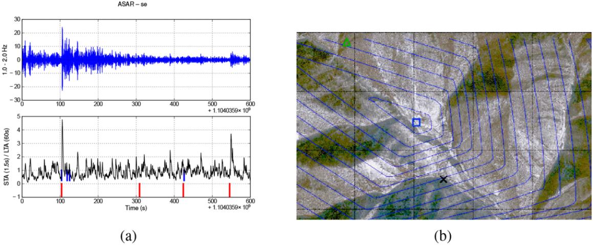
1. Top: Example of seismic waveform recorded at Alice Springs, Australia. Bottom: the waveform after processing to detect the arrival times of seismic waves. Blue lines are the automatically detected arrivals; red lines are the true arrivals. (b) Location estimates for the DPRK nuclear test of February 12, 2013: UN CTBTO Late Event Bulletin (green triangle at top left); NET-VISA (blue square in center). The entrance to the underground test facility (small “x”) is 0.75km from NET-VISA’s estimate. Contours show NET-VISA’s posterior location distribution. Courtesy of CTBTO Preparatory Commission.

Despite superficial differences, the two examples are structurally similar: there are unknown objects (papers, earthquakes) that generate percepts according to some physical process (citation, seismic propagation). The percepts are ambiguous as to their origin, but when multiple percepts are hypothesized to have originated with the same unknown object, that object’s properties can be inferred more accurately.

The same structure and reasoning patterns hold for areas such as database deduplication and natural language understanding. In some cases, inferring an object’s existence involves grouping percepts together—a process that resembles the clustering task in machine learning. In other cases, an object may generate no percepts at all and still have its existence inferred—as happened, for example, when observations of Uranus led to the discovery of Neptune. The existence of the unobserved object follows from its effects on the behavior and properties of observed objects.

15.3 Keeping Track of a Complex World

Chapter 14 considered the problem of keeping track of the state of the world, but covered only the case of atomic representations (HMMs) and factored representations (DBNs and Kalman filters). This makes sense for worlds with a single object—perhaps a single patient in the intensive care unit or a single bird flying through the forest. In this section, we see what happens when two or more objects generate the observations. What makes this case different from plain old state estimation is that there is now the possibility of uncertainty about which object generated which observation. This is the identity uncertainty problem of Section 15.2 (page 507), now viewed in a temporal context. In the control theory literature, this is the data association problem—that is, the problem of associating observation data with the objects that generated them. Although we could view this as yet another example of open-universe probabilistic modeling, it is important enough in practice to deserve its own section.

Data association

15.3.1 Example: Multitarget tracking

The data association problem was studied originally in the context of radar tracking of multiple targets, where reflected pulses are detected at fixed time intervals by a rotating radar antenna. At each time step, multiple blips may appear on the screen, but there is no direct observation of which blips at time correspond to which blips at time . Figure 15.8(a) shows a simple example with two blips per time step for five steps. Each blip is labeled with its time step but lacks any identifying information.

Figure 15.8

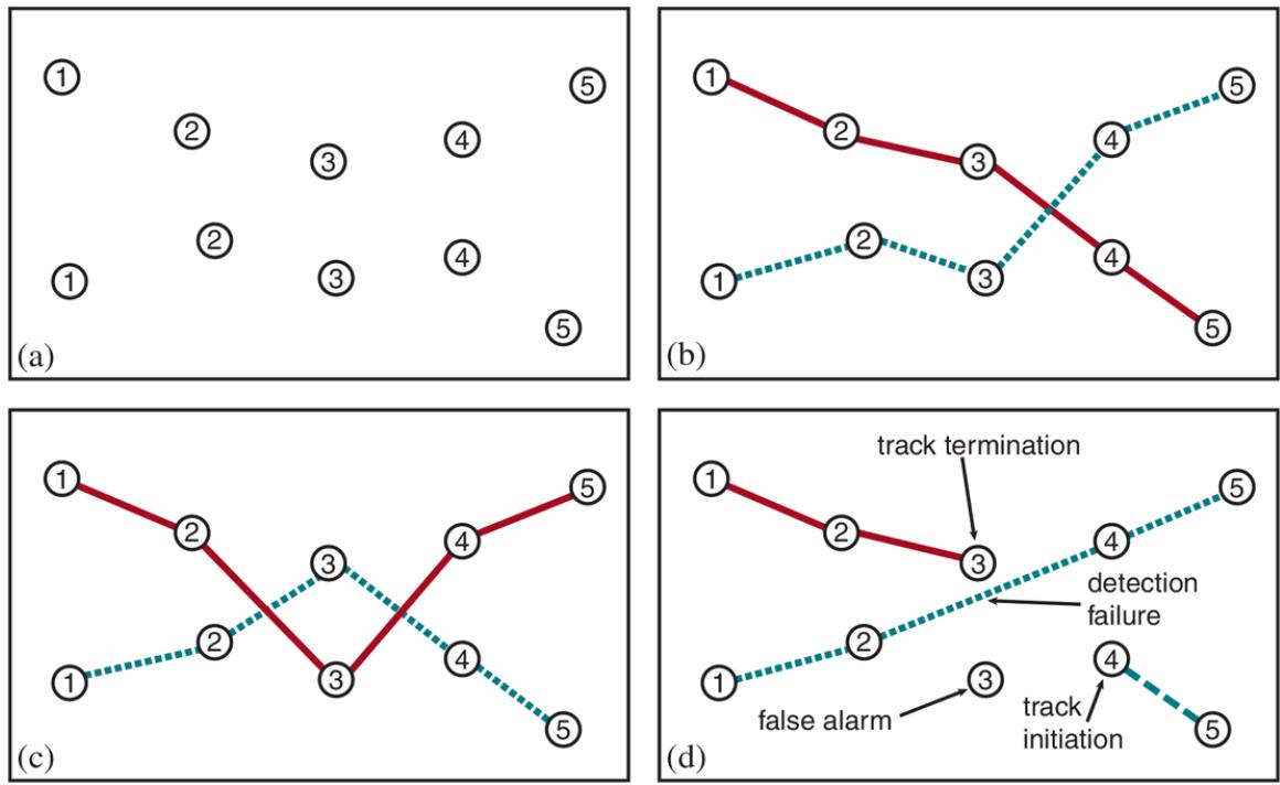
1. Observations made of object locations in 2D space over five time steps. Each observation blip is labeled with the time step but does not identify the object that produced it. (b–c) Possible hypotheses about the underlying object tracks. (d) A hypothesis for the case in which false alarms, detection failures, and track initiation/termination are possible.

Let us assume, for the time being, that we know there are exactly two aircraft, and , generating the blips. In the terminology of OUPMs, and are guaranteed objects, meaning that they are guaranteed to exist and to be distinct; moreover, in this case, there are no other objects. (In other words, as far as aircraft are concerned, this scenario matches the database semantics that is assumed in RPMs.) Let their true positions be and , where is a nonnegative integer that indexes the sensor update times. We assume the first observation arrives at , and at time 0 the prior distribution for every aircraft’s location is . Just to keep things simple, we’ll also assume that each aircraft moves independently according to a known transition model—e.g., a linear–Gaussian model as used in the Kalman filter (Section 14.4 ).

Guaranteed object

The final piece is the sensor model: again, we assume a linear–Gaussian model where an aircraft at position produces a blip whose observed blip position is a linear function of with added Gaussian noise. Each aircraft generates exactly one blip at each time step, so the blip has as its origins an aircraft and a time step. So, omitting the prior for now, the model looks like this:

where and are matrices describing the linear transition model and transition noise covariance, and and are the corresponding matrices for the sensor model. (See page 483.)

The key difference between this model and a standard Kalman filter is that there are two objects producing sensor readings (blips). This means there is uncertainty at any given time step about which object produced which sensor reading. Each possible world in this model includes an association—defined by values of all the variables for all the time steps —between aircraft and blips. Two possible association hypotheses are shown in Figure 15.8(b–c) . In general, for objects and time steps, there are ways of assigning blips to aircraft—an awfully large number.

The scenario described so far involved known objects generating observations at each time step. Real applications of data association are typically much more complicated. Often, the reported observations include false alarms (also known as clutter), which are not caused by real objects. Detection failures can occur, meaning that no observation is reported for a real object. Finally, new objects arrive and old ones disappear. These phenomena, which create even more possible worlds to worry about, are illustrated in Figure 15.8(d) . The corresponding OUPM is given in Figure 15.9 .

Figure 15.9

An OUPM for radar tracking of multiple targets with false alarms, detection failure, and entry and exit of aircraft. The rate at which new aircraft enter the scene is , while the probability per time step that an aircraft exits the scene is . False alarm blips (i.e., ones not produced by an aircraft) appear uniformly in space at a rate of per time step. The probability that an aircraft is detected (i.e., produces a blip) depends on its current position.

False alarm

Clutter

Detection failure

Because of its practical importance for both civilian and military applications, tens of thousands of papers have been written on the problem of multitarget tracking and data association. Many of them simply try to work out the complex mathematical details of the probability calculations for the model in Figure 15.9 , or for simpler versions of it. In one sense, this is unnecessary once the model is expressed in a probabilistic programming language, because the general-purpose inference engine does all of the mathematics correctly for any model—including this one. Furthermore, elaborations of the scenario (formation flying, objects heading for unknown destinations, objects taking off or landing, etc.) can be handled by small changes to the model without resorting to new mathematical derivations and complex programming.

From a practical point of view, the challenge with this kind of model is the complexity of inference. As for all probability models, inference means summing out the variables other than the query and the evidence. For filtering in HMMs and DBNs, we were able to sum out the state variables from 1 to by a simple dynamic programming trick; for Kalman filters, we also took advantage of special properties of Gaussians. For data association, we are less fortunate. There is no (known) efficient exact algorithm, for the same reason that there is none for the switching Kalman filter (page 484): the filtering distribution, which describes the joint distribution over numbers and locations of aircraft at each time step, ends up as a mixture of exponentially many distributions, one for each way of picking a sequence of observations to assign to each aircraft.

As a response to the complexity of exact inference, several approximate methods have been used. The simplest approach is to choose a single “best” assignment at each time step, given the predicted positions of the objects at the current time. This assignment associates observations with objects and enables the track of each object to be updated and a prediction made for the next time step. For choosing the “best” assignment, it is common to use the so-called nearest-neighbor filter, which repeatedly chooses the closest pairing of predicted position and observation and adds that pairing to the assignment. The nearestneighbor filter works well when the objects are well separated in state space and the prediction uncertainty and observation error are small—in other words, when there is no possibility of confusion.

Nearest-neighbor filter

When there is more uncertainty as to the correct assignment, a better approach is to choose the assignment that maximizes the joint probability of the current observations given the predicted positions. This can be done efficiently using the Hungarian algorithm (Kuhn, 1955), even though there are assignments to choose from as each new time step arrives.

Hungarian algorithm

Any method that commits to a single best assignment at each time step fails miserably under more difficult conditions. In particular, if the algorithm commits to an incorrect assignment, the prediction at the next time step may be significantly wrong, leading to more incorrect assignments, and so on. Sampling approaches can be much more effective. A particle filtering algorithm (see page 492) for data association works by maintaining a large collection of possible current assignments. An MCMC algorithm explores the space of assignment histories—for example, Figure 15.8(b–c) might be states in the MCMC state space—and can change its mind about previous assignment decisions.

One obvious way to speed up sampling-based inference for multitarget tracking is to use the Rao-Blackwellization trick from Chapter 14 (page 496): given a specific association hypothesis for all the objects, the filtering calculation for each object can typically be done exactly and efficiently, instead of sampling many possible state sequences for the objects. For example, with the model in Figure 15.9 , the filtering calculation just means running a Kalman filter for the sequence of observations assigned to a given hypothesized object. Furthermore, when changing from one association hypothesis to another, the calculations have to be redone only for objects whose associated observations have changed. Current MCMC data association methods can handle many hundreds of objects in real time while giving a good approximation to the true posterior distributions.

15.3.2 Example: Traffic monitoring

Figure 15.10 shows two images from widely separated cameras on a California freeway. In this application, we are interested in two goals: estimating the time it takes, under current traffic conditions, to go from one place to another in the freeway system; and measuring demand—that is, how many vehicles travel between any two points in the system at particular times of the day and on particular days of the week. Both goals require solving the data association problem over a wide area with many cameras and tens of thousands of vehicles per hour.

Figure 15.10

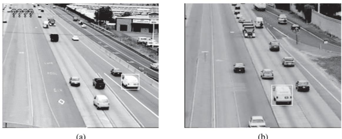
Images from (a) upstream and (b) downstream surveillance cameras roughly two miles apart on Highway 99 in Sacramento, California. The boxed vehicle has been identified at both cameras.

With visual surveillance, false alarms are caused by moving shadows, articulated vehicles, reflections in puddles, etc.; detection failures are caused by occlusion, fog, darkness, and lack of visual contrast; and vehicles are constantly entering and leaving the freeway system at points that may not be monitored. Furthermore, the appearance of any given vehicle can change dramatically between cameras depending on lighting conditions and vehicle pose in the image, and the transition model changes as traffic jams come and go. Finally, in dense traffic with widely separated cameras, the prediction error in the transition model for a car driving from one camera location to the next is far greater than the typical separation between vehicles. Despite these problems, modern data association algorithms have been successful in estimating traffic parameters in real-world settings.

Data association is an essential foundation for keeping track of a complex world, because without it there is no way to combine multiple observations of any given object. When objects in the world interact with each other in complex activities, understanding the world requires combining data association with the relational and open-universe probability models of Section 15.2 . This is currently an active area of research.

15.4 Programs as Probability Models

Many probabilistic programming languages have been built on the insight that probability models can be defined using executable code in any programming language that incorporates a source of randomness. For such models, the possible worlds are execution traces and the probability of any such trace is the probability of the random choices required for that trace to happen. PPLs created in this way inherit all of the expressive power of the underlying language, including complex data structures, recursion, and, in some cases, higher-order functions. Many PPLs are in fact computationally universal: they can represent any probability distribution that can be sampled from by a probabilistic Turing machine that halts.

15.4.1 Example: Reading text

We illustrate this approach to probabilistic modeling and inference via the problem of writing a program that reads degraded text. These kinds of models can be built for reading text that has been smudged or blurred due to water damage, or spotted due to aging of the paper on which it is printed. They can also be built for breaking some kinds of CAPTCHAs.

Figure 15.11 shows a generative program containing two components: (i) a way to generate a sequence of letters; and (ii) a way to generate a noisy, blurry rendering of these letters using an off-the-shelf graphics library. Figure 15.12 (top) shows example images generated by invoking GENERATE-IMAGE nine times.

Figure 15.11

Generative program for an open-universe probability model for optical character recognition. The generative program produces degraded images containing sequences of letters by generating each sequence, rendering it into a 2D image, and incorporating additive noise at each pixel.

Figure 15.12

The top panel shows twelve degraded images produced by executing the generative program from Figure 15.11 . The number of letters, their identities, the amount of additive noise, and the specific pixel-wise noise are all part of the domain of the probability model. The bottom panel shows twelve degraded images produced by executing the generative program from Figure 15.15 . The Markov model for letters typically yields sequences of letters that are easier to pronounce.

15.4.2 Syntax and semantics

A generative program is an executable program in which every random choice defines a random variable in an associated probability model. Let us imagine unrolling the execution of a program that makes random choices, step by step. Let be the random variable

corresponding to the th random choice made by the program; as usual, denotes a possible value of . Let us call an execution trace of the generative program—that is, a sequence of possible values for the random choices. Running the program once generates one such trace, hence the term “generative program.”

Generative program

Execution trace

The space of all possible execution traces can be viewed as the sample space of a probability model defined by the generative program. The probability distribution over traces can be defined as the product of the probabilities of each individual random choice: . This is analogous to the distribution over worlds in an OUPM.

It is conceptually straightforward to convert any OUPM into a corresponding generative program. This generative program makes random choices for each number statement and for the value of each basic random variable whose existence is implied by the number statements. The main extra work that the generative program needs to do is to create data structures that represent the objects, functions, and relations of the possible worlds in the OUPM. These data structures are created automatically by the OUPM inference engine because the OUPM assumes that every possible world is a first-order model structure, whereas a typical PPL makes no such assumption.

The images in Figure 15.12 can be used to get an intuitive understanding of the probability distribution : we see varying levels of noise, and in the less noisy images, we also see sequences of letters of varying lengths. Let be the trace corresponding to the image in the top right corner of this figure, containing the letters ocflwe. If we unrolled this trace into a Bayesian network, it would have 4,104 nodes: 1 node for the variable ; 6 nodes for the variables ; 1 node for the ; and 4,096 nodes for the pixels in . We thus see that this generative program defines an open-universe probability model: the

number of random choices it makes is not bounded a priori, but instead depends on the value of the random variable .

15.4.3 Inference results

Let’s apply this model to interpret images of letters that have been degraded with additive noise. Figure 15.13 shows a degraded image, along with results from three independent MCMC runs. For each run, we show a rendering of the letters contained in the trace after stopping the Markov chain. In all three cases the result is the letter sequence uncertainty, suggesting that the posterior distribution is highly concentrated on the correct interpretation.

Figure 15.13

Noisy input image (top) and inference results (bottom) produced by three runs, each of 25 MCMC iterations, with the model from Figure 15.11 . Note that the inference process correctly identifies the sequence of letters.

Now let’s degrade the text further, blurring it enough that it is difficult for people to read. Figure 15.14 shows the inference results on this more challenging input. This time, although MCMC inference appears to have converged on (what we know to be) the correct number of letters, the first letter is misidentified as a q and there is uncertainty about five of the ten following letters.

Figure 15.14

Top: extremely noisy input image. Bottom left: with three inference results from 25 MCMC iterations with the independent-letter model from Figure 15.11 . Bottom right: three inference results with the letter bigram model from Figure 15.15 . Both models exhibit ambiguity in the results, but the latter model’s results reflect prior knowledge of plausible letter sequences.

At this point, there are many possible ways to interpret the results. It could be that MCMC inference has mixed well and the results are a good reflection of the true posterior given the model and the image; in that case, the uncertainty in some of the letters and the error in the first letter are unavoidable. To get better results, we might need to improve the text model or reduce the noise level. It could also be that MCMC inference has not mixed properly: if we ran 300 chains for 25 thousand or 25 million iterations, we might find a quite different distribution of results, perhaps indicating that the first letter is probably u rather than q.

Running more inference could be costly in terms of dollars and waiting time. Moreover, there is no foolproof test for convergence of Monte Carlo inference methods. We could try to improve the inference algorithm, perhaps by designing a better proposal distribution for MCMC or using bottom-up clues from the image to suggest better initial hypotheses. These improvements require additional thought, implementation, and debugging. The third alternative is to improve the model. For example, we could incorporate knowledge about English words, such as the probabilities of letter pairs. We now consider this option.

15.4.4 Improving the generative program to incorporate a Markov model

Probabilistic programming languages are modular in a way that makes it easy to explore improvements to the underlying model. Figure 15.15 shows the generative program for an improved model that generates letters sequentially rather than independently. This

generative program uses a Markov model that draws each letter given the previous letter, with transition probabilities estimated from a reference list of English words.

Figure 15.15

Generative program for an improved optical character recognition model that generates letters according to a letter bigram model whose pairwise letter frequencies are estimated from a list of English words.

Figure 15.12 shows twelve sampled images produced by this generative program. Notice that the letter sequences are significantly more English-like than those generated from the program in Figure 15.11 . The right-hand panel in Figure 15.14 shows inference results from this Markov model applied to the high-noise image. The interpretations more closely match the generating trace, though there is still some uncertainty.

15.4.5 Inference in generative programs

As with OUPMs, exact inference in generative programs is usually prohibitively expensive or impossible. On the other hand, it is easy to see how to perform rejection sampling: run the program, keep just the traces that agree with the evidence, and count the different query answers found in those traces. Likelihood weighting is also straightforward: for each generated trace, keep track of the weight of the trace by multiplying all the probabilities of the values observed along the way.

Likelihood weighting works well only when the data are reasonably likely according to the model. In more difficult cases, MCMC is usually the method of choice. MCMC applied to probabilistic programs involves sampling and modifying execution traces. Many of the considerations arising with OUPMs also apply here; in addition, the algorithm has to be careful about modifications to an execution trace, such as changing the outcome of an ifstatement, that may invalidate the remainder of the trace.

Further improvements in inference come from several lines of work. Some improvements can produce fundamental shifts in the class of problems that are tractable with a given PPL, even in principle; lifted inference, described earlier for RPMs, can have this effect. In many cases, generic MCMC is too slow, and special-purpose proposals are needed to enable the inference process to mix quickly.

An important focus of recent work in PPLs has been to make it easy for users to define and use such proposals so that the efficiency of PPL inference matches that of custom inference algorithms devised for specific models.

Many promising approaches are aimed at reducing the overhead of probabilistic inference. The compilation idea described for Bayes nets in Section 13.4.3 can be applied to inference in OUPMs and PPLs, and typically yields speedups of two to three orders of magnitude. There have also been proposals for special-purpose hardware for algorithms such as messagepassing and MCMC. For example, Monte Carlo hardware exploits low-precision probability representations and massive fine-grained parallelism to deliver 100–10,000x improvements in speed and energy efficiency.

Methods based on learning can also give substantial improvements in speed. For example, adaptive proposal distributions can gradually learn how to generate MCMC proposals that are reasonably likely to be accepted and reasonably effective in exploring the probability landscape of the model to ensure rapid mixing. It is also possible to train deep learning models (see Chapter 21 ) to represent proposal distributions for importance sampling, using synthetic data that was generated from the underlying model.

Adaptive proposal distribution

In general, one expects that any formalism built on top of general programming languages will run up against the barrier of computability, and this is the case for PPLs. If we assume, however, that the underlying program halts for all inputs and all random choices, does the additional requirement of doing probabilistic inference still render the problem undecidable? It turns out that the answer is yes, but only for a computational model with

infinite-precision continuous random variables. In that case, it becomes possible to write a computable probability model in which inference encodes the halting problem. On the other hand, with finite-precision numbers and with the smooth probability distributions typically used in real applications, inference remains decidable.

Summary

This chapter has explored expressive representations for probability models based on both logic and programs.

• Relational probability models (RPMs) define probability models on worlds derived from the database semantics for first-order languages; they are appropriate when all the objects and their identities are known with certainty.
• Given an RPM, the objects in each possible world correspond to the constant symbols in the RPM, and the basic random variables are all possible instantiations of the predicate symbols with objects replacing each argument. Thus, the set of possible worlds is finite.
• RPMs provide very concise models for worlds with large numbers of objects and can handle relational uncertainty.
• Open-universe probability models (OUPMs) build on the full semantics of first-order logic, allowing for new kinds of uncertainty such as identity and existence uncertainty.
• Generative programs are representations of probability models—including OUPMs—as executable programs in a probabilistic programming language or PPL. A generative program represents a distribution over execution traces of the program. PPLs typically provide universal expressive power for probability models.

Bibliographical and Historical Notes

Hailperin (1984) and Howson (2003) recount the long history of attempts to connect probability and logic, going back to Leibniz’s Nouveaux Essais in 1704. These attempts usually involved probabilities attached directly to logical sentences. The first rigorous treatment was Gaifman’s propositional probability logic (Gaifman, 1964b). The idea is that a probability assertion is a constraint on the distribution over possible worlds, just as an ordinary logical sentence is a constraint on the possible worlds themselves. Any distribution that satisfies the constraint is a model, in the standard logical sense, of the probability assertion, and one probability assertion entails another just when the models of the first are a subset of the models of the second.

Probability logic

Within such a logic, one can prove, for example, that . Satisfiability of sets of probability assertions can be determined in the propositional case by linear programming (Hailperin, 1984; Nilsson, 1986). Thus, we have a “probability logic” in the same sense as “temporal logic”—a logical system specialized for probabilistic reasoning.

To apply probability logic to tasks such as proving interesting theorems in probability theory, a more expressive language was needed. Gaifman (1964a) proposed a first-order probability logic, with possible worlds being first-order model structures and with probabilities attached to sentences of (function-free) first-order logic. Scott and Krauss (1966) extended Gaifman’s results to allow infinite nesting of quantifiers and infinite sets of sentences.

Within AI, the most direct descendant of these ideas appears in probabilistic logic programs (Lukasiewicz, 1998), in which a probability range is attached to each first-order Horn clause and inference is performed by solving linear programs, as suggested by Hailperin. Halpern (1990) and Bacchus (1990) also built on Gaifman’s approach, exploring some of the basic knowledge representation issues from the perspective of AI rather than probability theory and mathematical logic.

The subfield of probabilistic databases also has logical sentences labeled with probabilities (Dalvi et al., 2009)—but in this case probabilities are attached directly to the tuples of the database. (In AI and statistics, probability is attached to general relationships, whereas observations are viewed as incontrovertible evidence.) Although probabilistic databases can model complex dependencies, in practice one often finds such systems using global independence assumptions across tuples.

Probabilistic databases

Attaching probabilities to sentences makes it very difficult to define complete and consistent probability models. Each inequality constrains the underlying probability model to lie in a half-space in the high-dimensional space of probability models. Conjoining assertions corresponds to intersecting the constraints. Ensuring that the intersection yields a single point is not easy. In fact, the principal result in Gaifman (1964a) is the construction of a single probability model requiring 1) a probability for every possible ground sentence and 2) probability constraints for infinitely many existentially quantified sentences.

One solution to this problem is to write a partial theory and then “complete” it by picking out one canonical model in the allowed set. Nilsson (1986) proposed choosing the maximum entropy model consistent with the specified constraints. Paskin (2002) developed a “maximum-entropy probabilistic logic” with constraints expressed as weights (relative probabilities) attached to first-order clauses. Such models are often called Markov logic networks or MLNs (Richardson and Domingos, 2006) and have become a popular technique for applications involving relational data. Maximum-entropy approaches, including MLNs, can produce unintuitive results in some cases (Milch, 2006; Jain et al., 2007, 2010).

Beginning in the early 1990s, researchers working on complex applications noticed the expressive limitations of Bayesian networks and developed various languages for writing “templates” with logical variables, from which large networks could be constructed automatically for each problem instance (Breese, 1992; Wellman et al., 1992). The most important such language was BUGS (Bayesian inference Using Gibbs Sampling) (Gilks et al., 1994; Lunn et al., 2013), which combined Bayesian networks with the indexed random variable notation common in statistics. (In BUGS, an indexed random variable looks like , where has a defined integer range.)

Indexed random variable

These closed-universe languages inherited the key property of Bayesian networks: every well-formed knowledge base defines a unique, consistent probability model. Other closeduniverse languages drew on the representational and inferential capabilities of logic programming (Poole, 1993; Sato and Kameya, 1997; Kersting et al., 2000) and semantic networks (Koller and Pfeffer, 1998; Pfeffer, 2000).

Research on open-universe probability models has several origins. In statistics, the problem of record linkage arises when data records do not contain standard unique identifiers—for example, various citations of this book might name its first author “Stuart J. Russell” or “S. Russell” or even “Stewart Russel.” Other authors share the name “S. Russell.”

Record linkage

Hundreds of companies exist solely to solve record linkage problems in financial, medical, census, and other data. Probabilistic analysis goes back to work by Dunn (1946); the Fellegi–Sunter model (1969), which is essentially naive Bayes applied to matching, still dominates current practice. Identity uncertainty is also considered in multitarget tracking (Sittler, 1964), whose history is sketched in Chapter 14 .

In AI, the working assumption until the 1990s was that sensors could supply logical sentences with unique identifiers for objects, as was the case with Shakey. In the area of natural language understanding, Charniak and Goldman (1992) proposed a probabilistic analysis of coreference, where two linguistic expressions (say, “Obama” and “the president”) may refer to the same entity. Huang and Russell (1998) and Pasula et al. (1999) developed a Bayesian analysis of identity uncertainty for traffic surveillance. Pasula et al. (2003) developed a complex generative model for authors, papers, and citation strings, involving both relational and identity uncertainty, and demonstrated high accuracy for citation information extraction.

The first formal language for open-universe probability models was BLOG (Milch et al., 2005; Milch, 2006), which came with a (very slow) general-purpose MCMC inference engine. Laskey (2008) describes another open-universe modeling language called multi-entity Bayesian networks. The NET-VISA global seismic monitoring system described in the text is due to Arora et al. (2013). The Elo rating system was developed in 1959 by Arpad Elo (1978) but is essentially the same at Thurstone’s Case V model (Thurstone, 1927). Microsoft’s TrueSkill model (Herbrich et al., 2007; Minka et al., 2018) is based on Mark Glickman’s (1999) Bayesian version of Elo and now runs on the infer.NET PPL.

Data association for multitarget tracking was first described in a probabilistic setting by Sittler (1964). The first practical algorithm for large-scale problems was the “multiple hypothesis tracker” or MHT algorithm (Reid, 1979). Important papers are collected by Bar-Shalom and Fortmann (1988) and Bar-Shalom (1992). The development of an MCMC algorithm for data association is due to Pasula et al. (1999), who applied it to traffic surveillance problems. Oh et al. (2009) provide a formal analysis and experimental comparisons to other methods. Schulz et al. (2003) describe a data association method based on particle filtering.

Ingemar Cox analyzed the complexity of data association (Cox, 1993; Cox and Hingorani, 1994) and brought the topic to the attention of the vision community. He also noted the applicability of the polynomial-time Hungarian algorithm to the problem of finding mostlikely assignments, which had long been considered an intractable problem in the tracking community. The algorithm itself was published by Kuhn (1955), based on translations of papers published in 1931 by two Hungarian mathematicians, Dénes König and Jenö

Egerváry. The basic theorem had been derived previously, however, in an unpublished Latin manuscript by the famous mathematician Carl Gustav Jacobi (1804–1851).

The idea that probabilistic programs could also represent complex probability models is due to Koller et al. (1997). The first working PPL was Avi Pfeffer’s IBAL (2001, 2007), based on a simple functional language. BLOG can be thought of as a declarative PPL. The connection between declarative and functional PPLs was explored by McAllester et al. (2008). CHURCH (Goodman et al., 2008), a PPL built on the Scheme language, pioneered the idea of piggybacking on an existing programming language. CHURCH also introduced the first MCMC inference algorithm for models with random higher-order functions and generated interest in the cognitive science community as a way to model complex forms of human learning (Lake et al., 2015). PPLs also connect in interesting ways to computability theory (Ackerman et al., 2013) and programming language research.

In the 2010s, dozens of PPLs emerged based on a wide range of underlying programming languages. Figaro, based on the Scala language, has been used for a wide variety of applications (Pfeffer, 2016). Gen (Cusumano-Towner et al., 2019), based on Julia and TensorFlow, has been used for real-time machine perception as well as Bayesian structure learning for time series data analysis. PPLs built on top of deep learning frameworks include Pyro (Bingham et al., 2019) (built on PyTorch) and Edward (Tran et al., 2017) (built on TensorFlow).

There have been efforts to make probabilistic programming accessible to more people, such as database and spreadsheet users. Tabular (Gordon et al., 2014) provides a spreadsheet-like relational schema language on top of infer.NET. BayesDB (Saad and Mansinghka, 2017) lets users combine and query probabilistic programs using an SQL-like language.

Inference in probabilistic programs has generally relied on approximate methods because exact algorithms do not scale to the kinds of models that PPLs can represent. Closeduniverse languages such as BUGS, LIBBI (Murray, 2013), and STAN (Carpenter et al., 2017) generally operate by constructing the full equivalent Bayesian network and then running inference on it—Gibbs sampling in the case of BUGS, sequential Monte Carlo in the case of LIBBI, and Hamiltonian Monte Carlo in the case of STAN. Programs in these languages can be read as instructions for building the ground Bayes net. Breese (1992) showed how to generate only the relevant fragment of the full network, given the query and the evidence.

Working with a grounded Bayes net means that the possible worlds visited by MCMC are represented by a vector of values for variables in the Bayes net. The idea of directly sampling first-order possible worlds is due to Russell (1999). In the FACTORIE language (McCallum et al., 2009), possible worlds in the MCMC process are represented within a standard relational database system. The same two papers propose incremental query reevaluation as a way to avoid full query evaluation on each possible world.

Inference methods based on grounding are analogous to the earliest propositionalization methods for first-order logical inference (Davis and Putnam, 1960). For logical inference, both resolution theorem provers and logic programming systems rely on lifting (Section 9.2 ) to avoid instantiating logical variables unnecessarily.

Pfeffer et al. (1999) introduced a variable elimination algorithm that cached each computed factor for reuse by later computations involving the same relations but different objects, thereby realizing some of the computational gains of lifting. The first truly lifted probabilistic inference algorithm was a form of variable elimination described by Poole (2003) and subsequently improved by de Salvo Braz et al. (2007). Further advances, including cases where certain aggregate probabilities can be computed in closed form, are described by Milch et al. (2008) and Kisynski and Poole, (2009). There is now a fairly good understanding of when lifting is possible and of its complexity (Gribkoff et al., 2014; Kazemi et al., 2017).

Methods of speeding up inference come in several flavors, as noted in the chapter. Several projects have explored more sophisticated algorithms, combined with compiler techniques and/or learned proposals. LIBBI (Murray, 2013) introduced the first particle Gibbs inference for probabilistic programs; one of the first inference compilers, with GPU support for massively parallel SMC; and use of the modeling language to define custom MCMC proposals. Compilation of probabilistic inference is also studied by Wingate et al. (2011), Paige and Wood (2014), Wu et al. (2016a). Claret et al. (2013), Hur et al. (2014), and Cusumano-Towner et al. (2019) demonstrate static analysis methods for transforming probabilistic programs into more efficient forms. PICTURE (Kulkarni et al. 2015) is the first PPL that let users apply learning from forward executions of the generative program to train fast bottom-up proposals. Le et al. (2017) describe the use of deep learning techniques for efficient importance sampling in a PPL. In practice, inference algorithms for complex probability models often use a mixture of techniques for different subsets of variables in the

model. Mansinghka et al. (2013) emphasized the idea of inference programs that apply diverse inference tactics to subsets of variables chosen during inference runtime.

The collection edited by Getoor and Taskar (2007) includes many important papers on firstorder probability models and their use in machine learning. Probabilistic programming papers appear in all the major conferences on machine learning and probabilistic reasoning, including NeurIPS, ICML, UAI, and AISTATS. Regular PPL workshops have been attached to the NeurIPS and POPL (Principles of Programming Languages) conferences, and the first International Conference on Probabilistic Programming was held in 2018.

Chapter 16 Making Simple Decisions

In which we see how an agent should make decisions so that it gets what it wants in an uncertain world—at least as much as possible and on average.

In this chapter, we fill in the details of how utility theory combines with probability theory to yield a decision-theoretic agent—an agent that can make rational decisions based on what it believes and what it wants. Such an agent can make decisions in contexts in which uncertainty and conflicting goals leave a logical agent with no way to decide. A goal-based agent has a binary distinction between good (goal) and bad (non-goal) states, while a decision-theoretic agent assigns a continuous range of values to states, and thus can more easily choose a better state even when no best state is available.

Section 16.1 introduces the basic principle of decision theory: the maximization of expected utility. Section 16.2 shows that the behavior of a rational agent can be modeled by maximizing a utility function. Section 16.3 discusses the nature of utility functions in more detail, and in particular their relation to individual quantities such as money. Section 16.4 shows how to handle utility functions that depend on several quantities. In Section 16.5 , we describe the implementation of decision-making systems. In particular, we introduce a formalism called a decision network (also known as an influence diagram) that extends Bayesian networks by incorporating actions and utilities. Section 16.6 hows how a decision-theoretic agent can calculate the value of acquiring new information to improve its decisions.

While Sections 16.1 –16.6 assume that the agent operates with a given, known utility function, Section 16.7 relaxes this assumption. We discuss the consequences of preference uncertainty on the part of the machine—the most important of which is deference to humans.

16.1 Combining Beliefs and Desires under Uncertainty

We begin with an agent that, like all agents, has to make a decision. It has available some actions . There may be uncertainty about the current state, so we’ll assume that the agent assigns a probability to each possible current state . There may also be uncertainty about the action outcomes; the transition model is given by , the probability that action in state reaches state . Because we’re primarily interested in the outcome , we’ll also use the abbreviated notation , the probability of reaching by doing in the current state, whatever that is. The two are related as follows:

\[P(\text{Resurr}(a) = s') = \sum\_{s} P(s)P\left(s'|s, a\right).\]

Decision theory, in its simplest form, deals with choosing among actions based on the desirability of their immediate outcomes; that is, the environment is assumed to be episodic in the sense defined on page 45. (This assumption is relaxed in Chapter 17 .) The agent’s preferences are captured by a utility function, , which assigns a single number to express the desirability of a state. The expected utility of an action given the evidence, , is just the average utility value of the outcomes, weighted by the probability that the outcome occurs:

(16.1)

\[EU(a) = \sum\_{s'} P\left(\text{RESULT}(a) = s'\right) U(s').\]

Utility function

Expected utility

The principle of maximum expected utility (MEU) says that a rational agent should choose the action that maximizes the agent’s expected utility:

\[action = \underset{\cdot}{\text{argmax}} \, EU(a).\]

In a sense, the MEU principle could be seen as a prescription for intelligent behavior. All an intelligent agent has to do is calculate the various quantities, maximize utility over its actions, and away it goes. But this does not mean that the AI problem is solved by the definition!

The MEU principle formalizes the general notion that an intelligent agent should “do the right thing,” but does not operationalize that advice. Estimating the probability distribution over possible states of the world, which folds into , requires perception, learning, knowledge representation, and inference. Computing itself requires a causal model of the world. There may be many actions to consider, and computing the outcome utilities may itself require further searching or planning because an agent may not know how good a state is until it knows where it can get to from that state. An AI system acting on behalf of a human may not know the human’s true utility function, so there may be uncertainty about . In summary, decision theory is not a panacea that solves the AI problem—but it does provide the beginnings of a basic mathematical framework that is general enough to define the AI problem.

The MEU principle has a clear relation to the idea of performance measures introduced in Chapter 2 . The basic idea is simple. Consider the environments that could lead to an agent having a given percept history, and consider the different agents that we could design. If an agent acts so as to maximize a utility function that correctly reflects the performance measure, then the agent will achieve the highest possible performance score (averaged over all the possible environments). This is the central justification for the MEU principle itself. While the claim may seem tautological, it does in fact embody a very important transition from the external performance measure to an internal utility function. The performance measure gives a score for a history—a sequence of states. Thus it is applied retrospectively after an agent completes a sequence of actions. The utility function applies to the very next state, so it can be used to guide actions step by step.

16.2 The Basis of Utility Theory

Intuitively, the principle of Maximum Expected Utility (MEU) seems like a reasonable way to make decisions, but it is by no means obvious that it is the only rational way. After all, why should maximizing the average utility be so special? What’s wrong with an agent that maximizes the weighted sum of the cubes of the possible utilities, or tries to minimize the worst possible loss? Could an agent act rationally just by expressing preferences between states, without giving them numeric values? Finally, why should a utility function with the required properties exist at all? We shall see.

16.2.1 Constraints on rational preferences

These questions can be answered by writing down some constraints on the preferences that a rational agent should have and then showing that the MEU principle can be derived from the constraints. We use the following notation to describe an agent’s preferences:

Now the obvious question is, what sorts of things are and ? They could be states of the world, but more often than not there is uncertainty about what is really being offered. For example, an airline passenger who is offered “the pasta dish or the chicken” does not know what lurks beneath the tinfoil cover. The pasta could be delicious or congealed, the chicken juicy or overcooked beyond recognition. We can think of the set of outcomes for each action as a lottery—think of each action as a ticket. A lottery with possible outcomes that occur with probabilities is written 1

1 We apologize to readers whose local airlines no longer offer food on long flights.

\[L = [p\_1, S\_1; \; p\_2, S\_2; \; \dots \; p\_n, S\_n].\]

In general, each outcome of a lottery can be either an atomic state or another lottery. The primary issue for utility theory is to understand how preferences between complex lotteries are related to preferences between the underlying states in those lotteries. To address this issue we list six constraints that we require any reasonable preference relation to obey:

ORDERABILITY: Given any two lotteries, a rational agent must either prefer one or else rate them as equally preferable. That is, the agent cannot avoid deciding. As noted on page 394, refusing to bet is like refusing to allow time to pass.

Orderability

TRANSITIVITY: Given any three lotteries, if an agent prefers to and prefers to , then the agent must prefer to .

\[(A \succ B) \land (B \succ C) \Rightarrow (A \succ C) \dots\]

Transitivity

CONTINUITY: If some lottery is between and in preference, then there is some probability for which the rational agent will be indifferent between getting for sure and the lottery that yields with probability and with probability .

\[A \succ B \succ C \Rightarrow \exists \; p \qquad [p, A; \; 1 - p, C] \sim B \; . .\]

Continuity

SUBSTITUTABILITY: If an agent is indifferent between two lotteries and , then the agent is indifferent between two more complex lotteries that are the same except that is substituted for in one of them. This holds regardless of the probabilities and the other outcome(s) in the lotteries.

\[A \sim B \Rightarrow [p, A; \ 1-p, C] \sim [p, B; 1-p, C] \ .\]

Substitutability

This also holds if we substitute for in this axiom.

MONOTONICITY: Suppose two lotteries have the same two possible outcomes, and . If an agent prefers to , then the agent must prefer the lottery that has a higher probability for (and vice versa).

\[A \succ B \Rightarrow (p > q \qquad \Leftrightarrow \qquad [p, A; \ 1 - p, B] \succ [q, A; \ 1 - q, B]).\]

Monotonicity

DECOMPOSABILITY: Compound lotteries can be reduced to simpler ones using the laws of probability. This has been called the “no fun in gambling” rule: as Figure 16.1(b) shows, it compresses two consecutive lotteries into a single equivalent lottery. 2

\[[p, A; \ 1-p, [q, B; \ 1-q, C]] \sim [p, A; \ (1-p)q, B; \ (1-p)(1-q), C].\]

Decomposability

² We can account for the enjoyment of gambling by encoding gambling events into the state description; for example, “Have and gambled” could be preferred to “Have and didn’t gamble.”

These constraints are known as the axioms of utility theory. Each axiom can be motivated by showing that an agent that violates it will exhibit patently irrational behavior in some situations. For example, we can motivate transitivity by making an agent with nontransitive preferences give us all its money. Suppose that the agent has the nontransitive preferences , where , , and are goods that can be freely exchanged. If the agent currently has , then we could offer to trade for plus one cent. The agent prefers , and so would be willing to make this trade. We could then offer to trade for , extracting another cent, and finally trade for . This brings us back where we started from, except that the agent has given us three cents (Figure 16.1(a) ). We can keep going around the cycle until the agent has no money at all. Clearly, the agent has acted irrationally in this case.

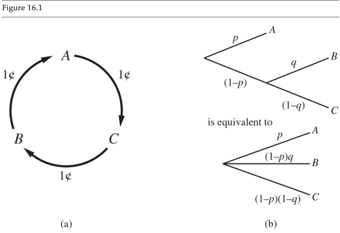
1. Nontransitive preferences can result in irrational behavior: a cycle of exchanges each costing one cent. (b) The decomposability axiom.

16.2.2 Rational preferences lead to utility

Notice that the axioms of utility theory are really axioms about preferences—they say nothing about a utility function. But in fact from the axioms of utility we can derive the following consequences (for the proof, see von Neumann and Morgenstern, 1944):

EXISTENCE OF UTILITY FUNCTION: If an agent’s preferences obey the axioms of utility, then there exists a function such that if and only if is preferred to , and if and only if the agent is indifferent between and . That is,

EXPECTED UTILITY OF A LOTTERY: The utility of a lottery is the sum of the probability of each outcome times the utility of that outcome.

\[U([p\_1, S\_1; \dots; p\_n, S\_n]) = \sum\_i p\_i U(S\_i).\]

In other words, once the probabilities and utilities of the possible outcome states are specified, the utility of a compound lottery involving those states is completely determined. Because the outcome of a nondeterministic action is a lottery, it follows that an agent can act rationally—that is, consistently with its preferences—only by choosing an action that maximizes expected utility according to Equation (16.1) .

The preceding theorems establish that (assuming the constraints on rational preferences) a utility function exists for any rational agent. The theorems do not establish that the utility function is unique. It is easy to see, in fact, that an agent’s behavior would not change if its utility function were transformed according to

(16.2)

\[U'(S) = aU(S) + b,\]

where and are constants and ; a positive affine transformation. This fact was noted in Chapter 5 (page 167) for two-player games of chance; here, we see that it applies to all kinds of decision scenarios. 3

As in game-playing, in a deterministic environment an agent needs only a preference ranking on states—the numbers don’t matter. This is called a value function or ordinal utility function.

³ In this sense, utilities resemble temperatures: a temperature in Fahrenheit is 1.8 times the Celsius temperature plus 32, but converting from one to the other doesn’t make you hotter or colder.

Value function

Ordinal utility function

It is important to remember that the existence of a utility function that describes an agent’s preference behavior does not necessarily mean that the agent is explicitly maximizing that utility function in its own deliberations. As we showed in Chapter 2 , rational behavior can be generated in any number of ways. A rational agent might be implemented with a table lookup (if the number of possible states is small enough).

By observing a rational agent’s behavior, an observer can learn about the utility function that represents what the agent is actually trying to achieve (even if the agent doesn’t know it). We return to this point in Section 16.7 .

16.3 Utility Functions

Utility functions map from lotteries to real numbers. We know they must obey the axioms of orderability, transitivity, continuity, substitutability, monotonicity, and decomposability. Is that all we can say about utility functions? Strictly speaking, that is it: an agent can have any preferences it likes. For example, an agent might prefer to have a prime number of dollars in its bank account; in which case, if it had it would give away . This might be unusual, but we can’t call it irrational. An agent might prefer a dented 1973 Ford Pinto to a shiny new Mercedes. The agent might prefer prime numbers of dollars only when it owns the Pinto, but when it owns the Mercedes, it might prefer more dollars to fewer. Fortunately, the preferences of real agents are usually more systematic and thus easier to deal with.

16.3.1 Utility assessment and utility scales

If we want to build a decision-theoretic system that helps a human make decisions or acts on his or her behalf, we must first work out what the human’s utility function is. This process, often called preference elicitation, involves presenting choices to the human and using the observed preferences to pin down the underlying utility function.

Preference elicitation

Equation (16.2) says that there is no absolute scale for utilities, but it is helpful, nonetheless, to establish some scale on which utilities can be recorded and compared for any particular problem. A scale can be established by fixing the utilities of any two particular outcomes, just as we fix a temperature scale by fixing the freezing point and boiling point of water. Typically, we fix the utility of a “best possible prize” at and a “worst possible catastrophe” at . (Both of these should be finite.) Normalized utilities use a scale with and . With such a scale, an England fan might assign a utility of 1 to England winning the World Cup and a utility of 0 to England failing to qualify.

Normalized utilities

Given a utility scale between and , we can assess the utility of any particular prize by asking the agent to choose between and a standard lottery . The probability is adjusted until the agent is indifferent between and the standard lottery. Assuming normalized utilities, the utility of is given by . Once this is done for each prize, the utilities for all lotteries involving those prizes are determined. Suppose, for example, we want to know how much our England fan values the outcome of England reaching the semifinal and then losing. We compare that outcome to a standard lottery with probability of winning the trophy and probability of an ignominious failure to qualify. If there is indifference at , then 0.3 is the value of reaching the semi-final and then losing.

Standard lottery

In medical, transportation, environmental and other decision problems, people’s lives are at stake. (Yes, there are things more important than England’s fortunes in the World Cup.) In such cases, is the value assigned to immediate death (or in the really worst cases, many deaths). Although nobody feels comfortable with putting a value on human life, it is a fact that tradeoffs on matters of life and death are made all the time. Aircraft are given a complete overhaul at intervals, rather than after every trip. Cars are manufactured in a way that trades off costs against accident survival rates. We tolerate a level of air pollution that kills four million people a year.

Paradoxically, a refusal to put a monetary value on life can mean that life is undervalued. Ross Shachter describes a government agency that commissioned a study on removing asbestos from schools. The decision analysts performing the study assumed a particular dollar value for the life of a school-age child, and argued that the rational choice under that assumption was to remove the asbestos. The agency, morally outraged at the idea of setting the value of a life, rejected the report out of hand. It then decided against asbestos removal —implicitly asserting a lower value for the life of a child than that assigned by the analysts.

Currently several agencies of the U.S. government, including the Environmental Protection Agency, the Food and Drug Administration, and the Department of Transportation, use the value of a statistical life to determine the costs and benefits of regulations and interventions. Typical values in 2019 are roughly .

Value of a statistical life

Micromort

Some attempts have been made to find out the value that people place on their own lives. One common “currency” used in medical and safety analysis is the micromort, a one in a million chance of death. If you ask people how much they would pay to avoid a risk—for example, to avoid playing Russian roulette with a million-barreled revolver—they will respond with very large numbers, perhaps tens of thousands of dollars, but their actual behavior reflects a much lower monetary value for a micromort.

For example, in the UK, driving in a car for 230 miles incurs a risk of one micromort. Over the life of your car—say, 92,000 miles—that’s 400 micromorts. People appear to be willing to pay about more for a safer car that halves the risk of death. Thus, their car-buying action says they have a value of per micromort. A number of studies have confirmed a figure in this range across many individuals and risk types. However, government agencies such as the U.S. Department of Transportation typically set a lower figure; they will spend only about in road repairs per expected life saved. Of course, these calculations hold only for small risks. Most people won’t agree to kill themselves, even for .

Another measure is the QALY, or quality-adjusted life year. Patients are willing to accept a shorter life expectancy to avoid a disability. For example, kidney patients on average are indifferent between living two years on dialysis and one year at full health.

16.3.2 The utility of money

Utility theory has its roots in economics, and economics provides one obvious candidate for a utility measure: money (or more specifically, an agent’s total net assets). The almost universal exchangeability of money for all kinds of goods and services suggests that money plays a significant role in human utility functions.

It will usually be the case that an agent prefers more money to less, all other things being equal. We say that the agent exhibits a monotonic preference for more money. This does not mean that money behaves as a utility function, because it says nothing about preferences between lotteries involving money.

Monotonic preference

Suppose you have triumphed over the other competitors in a television game show. The host now offers you a choice: either you can take the prize or you can gamble it on the flip of a coin. If the coin comes up heads, you end up with nothing, but if it comes up tails, you get . If you’re like most people, you would decline the gamble and pocket the million. Are you being irrational?

Assuming the coin is fair, the expected monetary value (EMV) of the gamble is which is more than the original . But that does not necessarily mean that accepting the gamble is a better decision. Suppose we use to denote the state of possessing total wealth , and that your current wealth is . Then the expected utilities of the two actions of accepting and declining the gamble are

To determine what to do, we need to assign utilities to the outcome states. Utility is not directly proportional to monetary value, because the utility for your first million is very high (or so they say), whereas the utility for an additional million is smaller. Suppose you assign a utility of 5 to your current financial status ( ), a 9 to the state , and an 8 to the state . Then the rational action would be to decline, because the expected utility of accepting is only 7 (less than the 8 for declining). On the other hand, a billionaire would most likely have a utility function that is locally linear over the range of a few million more, and thus would accept the gamble.

In a pioneering study of actual utility functions, Grayson (1960) found that the utility of money was almost exactly proportional to the logarithm of the amount. (This idea was first suggested by Bernoulli, (1738); see Exercise 16.STPT.) One particular utility curve, for a certain Mr. Beard, is shown in Figure 16.2(a) . The data obtained for Mr. Beard’s preferences are consistent with a utility function

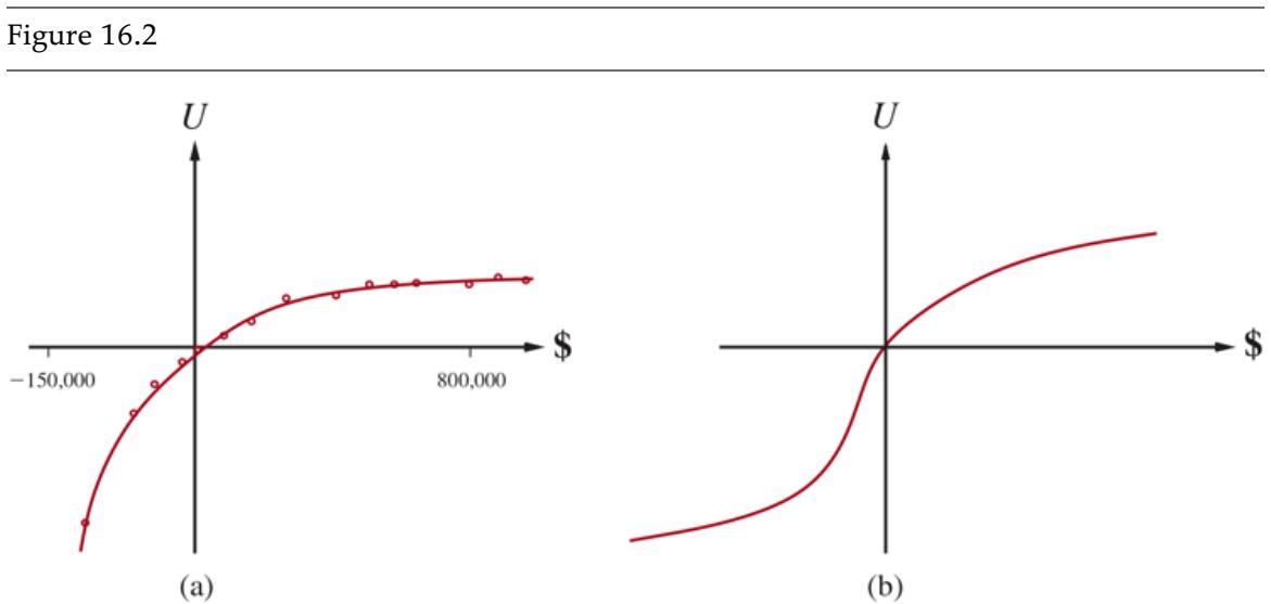
\[U(S\_{k+n}) = -263.31 + 22.09 \log(n + 150,000)\]

The utility of money. (a) Empirical data for Mr. Beard over a limited range. (b) A typical curve for the full range.

for the range between and .

We should not assume that this is the definitive utility function for monetary value, but it is likely that most people have a utility function that is concave for positive wealth. Going into debt is bad, but preferences between different levels of debt can display a reversal of the

concavity associated with positive wealth. For example, someone already in debt might well accept a gamble on a fair coin with a gain of for heads and a loss of for tails. This yields the S-shaped curve shown in Figure 16.2(b) . 4

4 Such behavior might be called desperate, but it is rational if one is already in a desperate situation.

If we restrict our attention to the positive part of the curves, where the slope is decreasing, then for any lottery , the utility of being faced with that lottery is less than the utility of being handed the expected monetary value of the lottery as a sure thing:

\[U(L) < U(S\_{EMV(L)}).\]

That is, agents with curves of this shape are risk-averse: they prefer a sure thing with a payoff that is less than the expected monetary value of a gamble. On the other hand, in the “desperate” region at large negative wealth in Figure 16.2(b) , the behavior is risk-seeking. The value an agent will accept in lieu of a lottery is called the certainty equivalent of the lottery. Studies have shown that most people will accept about in lieu of a gamble that gives half the time and the other half—that is, the certainty equivalent of the lottery is , while the EMV is .

Risk-averse

Risk-seeking

Certainty equivalent

Insurance premium

The difference between the EMV of a lottery and its certainty equivalent is called the insurance premium. Risk aversion is the basis for the insurance industry, because it means that insurance premiums are positive. People would rather pay a small insurance premium than gamble the price of their house against the chance of a fire. From the insurance company’s point of view, the price of the house is very small compared with the firm’s total reserves. This means that the insurer’s utility curve is approximately linear over such a small region, and the gamble costs the company almost nothing.

Notice that for small changes in wealth relative to the current wealth, almost any curve will be approximately linear. An agent that has a linear curve is said to be risk-neutral. For gambles with small sums, therefore, we expect risk neutrality. In a sense, this justifies the simplified procedure that proposed small gambles to assess probabilities and to justify the axioms of probability in Section 12.2.3 .

Risk-neutral

16.3.3 Expected utility and post-decision disappointment The rational way to choose the best action, , is to maximize expected utility:

\[a^\star = \underset{a}{\text{argmax}} \, EU(a).\]

If we have calculated the expected utility correctly according to our probability model, and if the probability model correctly reflects the underlying stochastic processes that generate the outcomes, then, on average, we will get the utility we expect if the whole process is repeated many times.

In reality, however, our model usually oversimplifies the real situation, either because we don’t know enough (e.g., when making a complex investment decision) or because the computation of the true expected utility is too difficult (e.g., when making a move in backgammon, needing to take into account all possible future dice rolls). In that case, we are really working with estimates of the true expected utility. We will assume, kindly perhaps, that the estimates are unbiased—that is, the expected value of the error,

, is zero. In that case, it still seems reasonable to choose the action with the highest estimated utility and to expect to receive that utility, on average, when the action is executed.

Unbiased

Unfortunately, the real outcome will usually be significantly worse than we estimated, even though the estimate was unbiased! To see why, consider a decision problem in which there are choices, each of which has true estimated utility of 0. Suppose that the error in each utility estimate is independent and has a unit normal distribution—that is, a Gaussian with zero mean and standard deviation of 1, shown as the bold curve in Figure 16.3 . Now, as we actually start to generate the estimates, some of the errors will be negative (pessimistic) and some will be positive (optimistic). Because we select the action with the highest utility estimate, we are favoring the overly optimistic estimates, and that is the source of the bias.

Figure 16.3

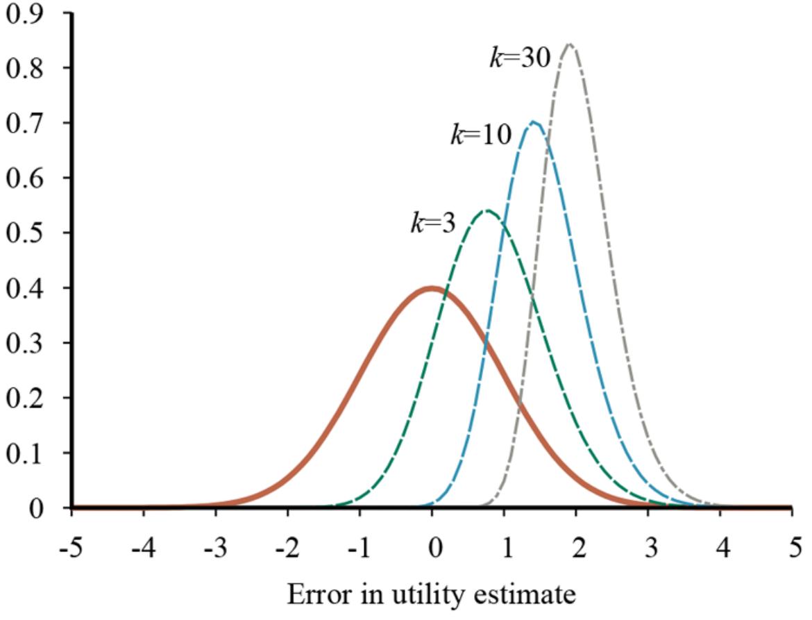
Unjustified optimism caused by choosing the best of options: we assume that each option has a true utility of 0 but a utility estimate that is distributed according to a unit normal (brown curve). The other curves show the distributions of the maximum of estimates for , 10, and 30.

It is a straightforward matter to calculate the distribution of the maximum of the estimates and hence quantify the extent of our disappointment. (This calculation is a special case of computing an order statistic, the distribution of any particular ranked element of a sample.) Suppose that each estimate has a probability density function and cumulative distribution . (As explained in Appendix A , the cumulative distribution measures the probability that the cost is less than or equal to any given amount—that is, it integrates the original density .) Now let be the largest estimate, i.e., . Then the cumulative distribution for is

\[\begin{aligned} P(\max\{X\_1, \dots, X\_k\} \le x) &= P(X\_1 \le x, \dots, X\_k \le x) \\ &= P(X\_1 \le x) \dots P(X\_k \le x) = F(x)^k, \end{aligned}\]

Order statistic

The probability density function is the derivative of the cumulative distribution function, so the density for , the maximum of estimates, is

\[P(x) = \frac{d}{dx}\left(F(x)^k\right) = kf(x)(F(x))^{k-1}.\]

These densities are shown for different values of in Figure 16.3 for the case where is the unit normal. For , the density for has a mean around 0.85, so the average disappointment will be about 85% of the standard deviation in the utility estimates. With more choices, extremely optimistic estimates are more likely to arise: for , the disappointment will be around twice the standard deviation in the estimates.

This tendency for the estimated expected utility of the best choice to be too high is called the optimizer’s curse (Smith and Winkler, 2006). It afflicts even the most seasoned decision analysts and statisticians. Serious manifestations include believing that an exciting new drug that has cured 80% of patients in a trial will cure 80% of patients (it’s been chosen from thousands of candidate drugs) or that a mutual fund advertised as having above-average returns will continue to have them (it’s been chosen to appear in the advertisement out of dozens of funds in the company’s overall portfolio). It can even be the case that what appears to be the best choice may not be, if the variance in the utility estimate is high: a drug that has cured 9 of 10 patients and has been selected from thousands tried is probably worse than one that has cured 800 of 1000.

Optimizer’s curse

The optimizer’s curse crops up everywhere because of the ubiquity of utility-maximizing selection processes, so taking the utility estimates at face value is a bad idea. We can avoid the curse with a Bayesian approach that uses an explicit probability model of the error in the utility estimates. Given this model and a prior on what we might reasonably expect the utilities to be, we treat the utility estimate as evidence and compute the posterior distribution for the true utility using Bayes’ rule.

16.3.4 Human judgment and irrationality

Decision theory is a normative theory: it describes how a rational agent should act. A descriptive theory, on the other hand, describes how actual agents—for example, humans really do act. The application of economic theory would be greatly enhanced if the two coincided, but there appears to be some experimental evidence to the contrary. The evidence suggests that humans are “predictably irrational” (Ariely, 2009).

Normative theory

Descriptive theory

The best-known problem is the Allais paradox (Allais, 1953). People are given a choice between lotteries and and then between and , which have the following prizes:

Most people consistently prefer over (taking the sure thing), and over (taking the higher EMV). The normative analysis disagrees! We can see this most easily if we use the freedom implied by Equation (16.2) to set . In that case, then implies that , whereas implies exactly the reverse. In other words, there is no utility function that is consistent with these choices.

One explanation for the apparently irrational preferences is the certainty effect (Kahneman and Tversky, 1979): people are strongly attracted to gains that are certain. There are several reasons why this may be so.

Certainty effect

First, people may prefer to reduce their computational burden; by choosing certain outcomes, they don’t have to compute with probabilities. But the effect persists even when the computations involved are very easy ones.

Second, people may distrust the legitimacy of the stated probabilities. I trust that a coin flip is roughly if I have control over the coin and the flip, but I may distrust the result if the flip is done by someone with a vested interest in the outcome. In the presence of distrust, it might be better to go for the sure thing. 5 6

5 For example, the mathematician/magician Persi Diaconis can make a coin flip come out the way he wants every time (Landhuis, 2004).

6 Even the sure thing may not be certain. Despite cast-iron promises, we have not yet received that from the Nigerian bank account of a previously unknown deceased relative.

Third, people may be accounting for their emotional state as well as their financial state. People know they would experience regret if they gave up a certain reward ( ) for an 80% chance at a higher reward and then lost.

In other words, if is chosen, there is a 20% chance of getting no money and feeling like a complete idiot, which is worse than just getting no money. So perhaps people who choose over and over are not irrational; they are willing to give up of EMV to avoid a 20% chance of feeling like an idiot.

A related problem is the Ellsberg paradox. Here the prizes are fixed, but the probabilities are underconstrained. Your payoff will depend on the color of a ball chosen from an urn. You are told that the urn contains red balls, and either black or yellow balls, but you don’t know how many black and how many yellow. Again, you are asked whether you prefer lottery or ; and then or :

It should be clear that if you think there are more red than black balls then you should prefer over and over ; if you think there are fewer red than black you should prefer the opposite. But it turns out that most people prefer over and also prefer over , even though there is no state of the world for which this is rational. It seems that people have ambiguity aversion: gives you a chance of winning, while could be anywhere between 0 and . Similarly, gives you a chance, while could be anywhere between and . Most people elect the known probability rather than the unknown unknowns.

Ambiguity aversion

Yet another problem is that the exact wording of a decision problem can have a big impact on the agent’s choices; this is called the framing effect. Experiments show that people like a medical procedure that is described as having a “90% survival rate” about twice as much as one described as having a “10% death rate,” even though these two statements mean exactly the same thing. This discrepancy in judgment has been found in multiple experiments and is about the same whether the subjects are patients in a clinic, statistically sophisticated business school students, or experienced doctors.

Framing effect

People feel more comfortable making relative utility judgments rather than absolute ones. I may have little idea how much I might enjoy the various wines offered by a restaurant. The restaurant takes advantage of this by offering a bottle that nobody will buy, but which serves to skew upward the customer’s estimate of the value of all wines, making a bottle seem like a bargain. This is called the anchoring effect.

Anchoring effect

If human informants insist on contradictory preference judgments, there is nothing that automated agents can do to be consistent with them. Fortunately, preference judgments made by humans are often open to revision in the light of further consideration. Paradoxes like the Allais and Ellsberg paradoxes are greatly reduced (but not eliminated) if the choices are explained better. In work at the Harvard Business School on assessing the utility of money, Keeney and Raiffa (1976 p. 210) found the following:

Subjects tend to be too risk-averse in the small and therefore the fitted utility functions exhibit unacceptably large risk premiums for lotteries with a large spread. Most of the subjects, however, can reconcile their inconsistencies and feel that they have learned an important lesson about how they want to behave. As a consequence, some subjects cancel their automobile collision insurance and take out more term insurance on their lives.

The evidence for human irrationality is also questioned by researchers in the field of evolutionary psychology, who point to the fact that our brain’s decision-making mechanisms did not evolve to solve word problems with probabilities and prizes stated as decimal numbers. Let us grant, for the sake of argument, that the brain has built-in neural mechanisms for computing with probabilities and utilities, or something functionally equivalent. If so, the required inputs would be obtained through accumulated experience of outcomes and rewards rather than through linguistic presentations of numerical values.

Evolutionary psychology

It is far from obvious that we can directly access the brain’s built-in neural mechanisms by presenting decision problems in linguistic/numerical form. The very fact that different wordings of the same decision problem elicit different choices suggests that the decision problem itself is not getting through. Spurred by this observation, psychologists have tried presenting problems in uncertain reasoning and decision making in “evolutionarily appropriate” forms; for example, instead of saying “90% survival rate,” the experimenter might show 100 stick-figure animations of the operation, where the patient dies in 10 of

them and survives in 90. With decision problems posed in this way, people’s behavior seems to be much closer to the standard of rationality.

16.4 Multiattribute Utility Functions

Decision making in the field of public policy involves high stakes, in both money and lives. For example, in deciding what levels of harmful emissions to allow from a power plant, policy makers must weigh the prevention of death and disability against the benefit of the power and the economic burden of mitigating the emissions. Picking a site for a new airport requires consideration of the disruption caused by construction; the cost of land; the distance from centers of population; the noise of flight operations; safety issues arising from local topography and weather conditions; and so on. Problems like these, in which outcomes are characterized by two or more attributes, are handled by multiattribute utility theory. In essence, it’s the theory of comparing apples to oranges.

Multiattribute utility theory

Let the attributes be and let be a complete vector of assignments, where each is either a numeric value or a discrete value with an assumed ordering on values. The analysis is easier if we arrange it so that higher values of an attribute always correspond to higher utilities: utilities are monotonically increasing. That means that we can’t use, say, the number of deaths, as an attribute; we would have to use . It also means that we can’t use the room temperature, , as an attribute. If the utility function for temperature has a peak at F and falls off monotonically on either side, then we could split the attribute into two pieces. We could use to measure whether the room is warm enough, and to measure whether it is cool enough; both of these attributes would be monotonically increasing until they reach their maximum utility value at 0; the utility curve is flat from that point on, meaning that you dont’t get any more “warm enough” above , nor any more “cool enough” below .

The attributes in the airport problem could be:

THROUGHPUT, measured by the number of flights per day;

• SAFETY, measured by minus the expected number of deaths per year;
• QUIETNESS, measured by minus the number of people living under the flight paths;
• FRUGALITY, measured by the negative cost of construction.

We begin by examining cases in which decisions can be made without combining the attribute values into a single utility value. Then we look at cases in which the utilities of attribute combinations can be specified very concisely.

16.4.1 Dominance

Suppose that airport site costs less, generates less noise pollution, and is safer than site . One would not hesitate to reject . We then say that there is strict dominance of over . In general, if an option is of lower value on all attributes than some other option, it need not be considered further. Strict dominance is often very useful in narrowing down the field of choices to the real contenders, although it seldom yields a unique choice. Figure 16.4(a) shows a schematic diagram for the two-attribute case.

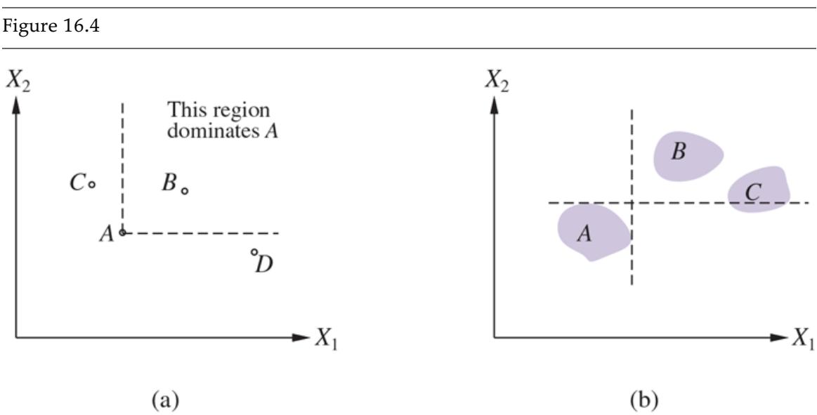
Strict dominance. (a) Deterministic: Option A is strictly dominated by B but not by C or D. (b) Uncertain: A is strictly dominated by B but not by C.

Strict dominance

That is fine for the deterministic case, in which the attribute values are known for sure. What about the general case, where the outcomes are uncertain? A direct analog of strict dominance can be constructed, where, despite the uncertainty, all possible concrete outcomes for strictly dominate all possible outcomes for . (See Figure 16.4(b) .) Of course, this will probably occur even less often than in the deterministic case.

Fortunately, there is a more useful generalization called stochastic dominance, which occurs very frequently in real problems. Stochastic dominance is easiest to understand in the context of a single attribute. Suppose we believe that the cost of placing the airport at is uniformly distributed between billion and billion and that the cost at is uniformly distributed between billion and billion. Define the Frugality attribute to be the negative cost. Figure 16.5(a) shows the distributions for the frugality of sites and . Then, given only the information that the more frugal choice is better (all other things being equal), we can say that stochastically dominates (i.e., can be discarded). It is important to note that this does not follow from comparing the expected costs. For example, if we knew the cost of to be exactly billion, then we would be unable to make a decision without additional information on the utility of money. (It might seem odd that more information on the cost of could make the agent less able to decide. The paradox is resolved by noting that in the absence of exact cost information, the decision is easier to make but is more likely to be wrong.)

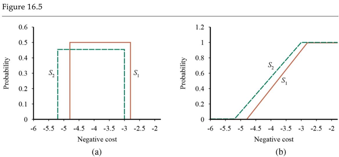
Stochastic dominance. (a) stochastically dominates on frugality (negative cost). (b) Cumulative distributions for the frugality of and .

The exact relationship between the attribute distributions needed to establish stochastic dominance is best seen by examining the cumulative distributions, shown in Figure 16.5(b) . If the cumulative distribution for is always to the right of the cumulative distribution for , then, stochastically speaking, is cheaper than . Formally, if two actions and lead to probability distributions and on attribute , then stochastically dominates on if

\[\forall x \qquad \int\_{-\infty}^{x} p\_1(x') \quad dx' \le \int\_{-\infty}^{x} p\_2(x') \quad dx'.\]

The relevance of this definition to the selection of optimal decisions comes from the following property: if stochastically dominates , then for any monotonically nondecreasing utility function , the expected utility of is at least as high as the expected utility of . To see why this is true, consider the two expected utilities, and . Initially, it’s not obvious why the first integral is bigger than the second, given that the stochastic dominance condition has a -integral that is smaller than the -integral.

Instead of thinking about the integral over , however, think about the integral over , the cumulative probability, as shown in Figure 16.5(b) . For any value of , the corresponding value of (and hence of ) is bigger for than for ; so if we integrate a bigger quantity over the whole range of , we are bound to get a bigger result. Formally, it’s just a substitution of in the integral for ’s expected value and in the integral for ’s. With these substitutions, we have for and for , hence

\[\int\_{-\infty}^{\infty} p\_1(x)U(x)dx = \int\_0^1 U(P\_1^{-1}(y))dy \ge \int\_0^1 U(P\_2^{-1}(y))dy = \int\_{-\infty}^{\infty} p\_2(x)U(x)dx.\]

This inequality allows us to prefer to in a single-attribute problem. More generally, if an action is stochastically dominated by another action on all attributes in a multiattribute problem, then it can be discarded.

The stochastic dominance condition might seem rather technical and perhaps not so easy to evaluate without extensive probability calculations. In fact, it can be decided very easily in

many cases. For example, would you rather fall head-first onto concrete from 3 millimeters or 3 meters? Assuming you chose 3 millimeters—good choice! Why is it necessarily a better decision? There is a good deal of uncertainty about the degree of damage you will incur in both cases; but for any given level of damage, the probability that you’ll incur at least that level of damage is higher when falling from 3 meters than from 3 millimeters. In other words, 3 millimeters stochastically dominates 3 meters on the Safety attribute.

This kind of reasoning comes as second nature to humans; it’s so obvious we don’t even think about it. Stochastic domination abounds in the airport problem too. Suppose, for example, that the construction transportation cost depends on the distance to the supplier. The cost itself is uncertain, but the greater the distance, the greater the cost. If is closer than , then will dominate on frugality. Although we will not present them here, algorithms exist for propagating this kind of qualitative information among uncertain variables in qualitative probabilistic networks, enabling a system to make rational decisions based on stochastic dominance, without using any numeric values.

Qualitative probabilistic networks

16.4.2 Preference structure and multiattribute utility

Suppose we have attributes, each of which has distinct possible values. To specify the complete utility function , we need values in the worst case. Multiattribute utility theory aims to identify additional structure in human preferences so that we don’t need to specify all values individually. Having identified some regularity in preference behavior, we then derive representation theorems to show that an agent with a certain kind of preference structure has a utility function

\[U(x\_1, \ldots, x\_n) = F[f\_1(x\_1), \ldots, f\_n(x\_n)],\]

Representation theorem

where is (we hope) a simple function such as addition. Notice the similarity to the use of Bayesian networks to decompose the joint probability of several random variables.

As an example, suppose each is the amount of money the agent has in a particular currency: dollars, euros, marks, lira, etc. The functions could then convert each amount into a common currency, and would then be simply addition.

Preferences without uncertainty

Let us begin with the deterministic case. On page 532 we noted that for deterministic environments, the agent has a value function, which we write here as ; the aim is to represent this function concisely. The basic regularity that arises in deterministic preference structures is called preference independence. Two attributes and are preferentially independent of a third attribute if the preference between outcomes and does not depend on the particular value for attribute .

Preference independence

Going back to the airport example, where we have (among other attributes) Quietness, Frugality, and Safety to consider, one may propose that Quietness and Frugality are preferentially independent of Safety. For example, if we prefer an outcome with 20,000 people residing in the flight path and a construction cost of billion over an outcome with 70,000 people residing in the flight path and a cost of billion when the safety level is 0.006 deaths per billion passenger miles in both cases, then we would have the same preference when the safety level is 0.012 or 0.003; and the same independence would hold for preferences between any other pair of values for Quietness and Frugality. It is also apparent that Frugality and Safety are preferentially independent of Quietness and that Quietness and Safety are preferentially independent of Frugality.

We say that the set of attributes exhibits mutual preferential independence (MPI). MPI says that, whereas each attribute may be important, it does not affect the way in which one trades off the other attributes against each other.

Mutual preferential independence (MPI)

Mutual preferential independence is a complicated name, but it leads to a simple form for the agent’s value function (Debreu, 1960): If attributes are mutually preferentially independent, then the agent’s preferences can be represented by a value function

\[V(x\_1, \ldots, x\_n) = \sum\_{i} V\_i(x\_i),\]

where each refers only to the attribute . For example, it might well be the case that the airport decision can be made using a value function

Additive value function

A value function of this type is called an additive value function. Additive functions are an extremely natural way to describe an agent’s preferences and are valid in many real-world situations. For attributes, assessing an additive value function requires assessing separate one-dimensional value functions rather than one -dimensional function; typically, this represents an exponential reduction in the number of preference experiments that are needed. Even when MPI does not strictly hold, as might be the case at extreme values of the attributes, an additive value function might still provide a good approximation to the agent’s preferences. This is especially true when the violations of MPI occur in portions of the attribute ranges that are unlikely to occur in practice.

To understand MPI better, it helps to look at cases where it doesn’t hold. Suppose you are at a medieval market, considering the purchase of some hunting dogs, some chickens, and some wicker cages for the chickens. The hunting dogs are very valuable, but if you don’t have enough cages for the chickens, the dogs will eat the chickens; hence, the tradeoff between dogs and chickens depends strongly on the number of cages, and MPI is violated.

The existence of these kinds of interactions among various attributes makes it much harder to assess the overall value function.

Preferences with uncertainty

When uncertainty is present in the domain, we also need to consider the structure of preferences between lotteries and to understand the resulting properties of utility functions, rather than just value functions. The mathematics of this problem can become quite complicated, so we present just one of the main results to give a flavor of what can be done.

The basic notion of utility independence extends preference independence to cover lotteries: a set of attributes is utility independent of a set of attributes if preferences between lotteries on the attributes in are independent of the particular values of the attributes in . A set of attributes is mutually utility independent (MUI) if each of its subsets is utility-independent of the remaining attributes. Again, it seems reasonable to propose that the airport attributes are MUI.

Utility independence

Mutually utility independent

MUI implies that the agent’s behavior can be described using a multiplicative utility function (Keeney, 1974). The general form of a multiplicative utility function is best seen by looking at the case for three attributes. For conciseness, we use to mean :

\[\begin{aligned} U &= \begin{aligned} k\_1 U\_1 + k\_2 U\_2 + k\_3 U\_3 + k\_1 k\_2 U\_1 U\_2 + k\_2 k\_3 U\_2 U\_3 + k\_3 k\_1 U\_3 U\_1 \\ + k\_1 k\_2 k\_3 U\_1 U\_2 U\_3. \end{aligned} \end{aligned}\]

Multiplicative utility function

Although this does not look very simple, it contains just three single-attribute utility functions and three constants. In general, an -attribute problem exhibiting MUI can be modeled using single-attribute utilities and constants. Each of the single-attribute utility functions can be developed independently of the other attributes, and this combination will be guaranteed to generate the correct overall preferences. Additional assumptions are required to obtain a purely additive utility function.

16.5 Decision Networks

Influence diagram

Decision network

In this section, we look at a general mechanism for making rational decisions. The notation is often called an influence diagram (Howard and Matheson, 1984), but we will use the more descriptive term decision network. Decision networks combine Bayesian networks with additional node types for actions and utilities. We use the problem of picking an airport site as an example.

16.5.1 Representing a decision problem with a decision network

In its most general form, a decision network represents information about the agent’s current state, its possible actions, the state that will result from the agent’s action, and the utility of that state. It therefore provides a substrate for implementing utility-based agents of the type first introduced in Section 2.4.5 . Figure 16.6 shows a decision network for the airport-siting problem. It illustrates the three types of nodes used:

Chance nodes (ovals) represent random variables, just as they do in Bayesian networks. The agent could be uncertain about the construction cost, the level of air traffic and the potential for litigation, and the Safety, Quietness, and total Frugality variables, each of which also depends on the site chosen. Each chance node has associated with it a conditional distribution that is indexed by the state of the parent nodes. In decision networks, the parent nodes can include decision nodes as well as chance nodes. Note that each of the current-state chance nodes could be part of a large Bayesian network for assessing construction costs, air traffic levels, or litigation potentials.

Chance nodes

Decision nodes (rectangles) represent points where the decision maker has a choice of actions. In this case, the AirportSite action can take on a different value for each site under consideration. The choice influences the safety, quietness, and frugality of the solution. In this chapter, we assume that we are dealing with a single decision node. Chapter 17 deals with cases in which more than one decision must be made.

Decision nodes

Utility nodes (diamonds) represent the agent’s utility function. The utility node has as parents all variables describing the outcomes that directly affect utility. Associated with the utility node is a description of the agent’s utility as a function of the parent attributes. The description could be just a tabulation of the function, or it might be a parameterized additive or linear function of the attribute values. For now, we will assume that the function is deterministic; that is, given the values of its parent variables, the value of the utility node is fully determined. 7

7 These nodes are also called value nodes in the literature.

Utility nodes

Figure 16.6

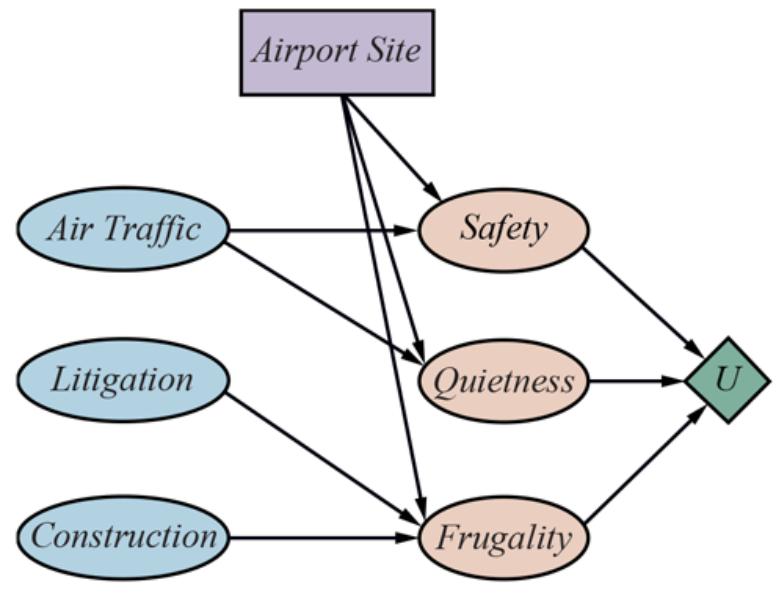
A decision network for the airport-siting problem.

A simplified form is also used in many cases. The notation remains identical, but the chance nodes describing the outcome states are omitted. Instead, the utility node is connected directly to the current-state nodes and the decision node. In this case, rather than representing a utility function on outcome states, the utility node represents the expected utility associated with each action, as defined in Equation (16.1) on page 529; that is, the node is associated with an action-utility function (also known as a Q-function in reinforcement learning, as described in Chapter 22 ). Figure 16.7 shows the action-utility representation of the airport siting problem.

Figure 16.7

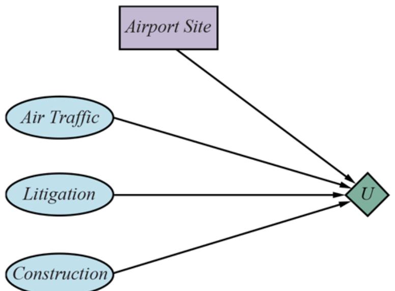
A simplified representation of the airport-siting problem. Chance nodes corresponding to outcome states have been factored out.

Action-utility function

Notice that, because the Quietness, Safety, and Frugality chance nodes in Figure 16.6 refer to future states, they can never have their values set as evidence variables. Thus, the simplified version that omits these nodes can be used whenever the more general form can be used. Although the simplified form contains fewer nodes, the omission of an explicit description of the outcome of the siting decision means that it is less flexible with respect to changes in circumstances.

For example, in Figure 16.6 , a change in aircraft noise levels can be reflected by a change in the conditional probability table associated with the Quietness node, whereas a change in the weight accorded to noise pollution in the utility function can be reflected by a change in the utility table. In the action-utility diagram, Figure 16.7 , on the other hand, all such changes have to be reflected by changes to the action-utility table. Essentially, the actionutility formulation is a compiled version of the original formulation, obtained by summing out the outcome state variables.

16.5.2 Evaluating decision networks

Actions are selected by evaluating the decision network for each possible setting of the decision node. Once the decision node is set, it behaves exactly like a chance node that has been set as an evidence variable. The algorithm for evaluating decision networks is the following:

• 1. Set the evidence variables for the current state.
• 2. For each possible value of the decision node:
  • a. Set the decision node to that value.
  • b. Calculate the posterior probabilities for the parent nodes of the utility node, using a standard probabilistic inference algorithm.
  • c. Calculate the resulting utility for the action.
• 3. Return the action with the highest utility.

This is a straightforward approach that can utilize any available Bayesian network algorithm and can be incorporated directly into the agent design given in Figure 12.1 on page 388. We will see in Chapter 17 that the possibility of executing several actions in sequence makes the problem much more interesting.

16.6 The Value of Information

In the preceding analysis, we have assumed that all relevant information, or at least all available information, is provided to the agent before it makes its decision. In practice, this is hardly ever the case. One of the most important parts of decision making is knowing what questions to ask. For example, a doctor cannot expect to be provided with the results of all possible diagnostic tests and questions at the time a patient first enters the consulting room. Tests are often expensive and sometimes hazardous (both directly and because of associated delays). Their importance depends on two factors: whether the test results would lead to a significantly better treatment plan, and how likely the various test results are.

This section describes information value theory, which enables an agent to choose what information to acquire. We assume that prior to selecting a “real” action represented by the decision node, the agent can acquire the value of any of the potentially observable chance variables in the model. Thus, information value theory involves a simplified form of sequential decision making—simplified because the observation actions affect only the agent’s belief state, not the external physical state. The value of any particular observation must derive from the potential to affect the agent’s eventual physical action; and this potential can be estimated directly from the decision model itself.

Information value theory

16.6.1 A simple example

Suppose an oil company is hoping to buy one of indistinguishable blocks of ocean-drilling rights. Let us assume further that exactly one of the blocks contains oil that will generate net profits of dollars, while the others are worthless. The asking price of each block is dollars. If the company is risk-neutral, then it will be indifferent between buying a block and not buying one because the expected profit is zero in both cases.

Now suppose that a seismologist offers the company the results of a survey of block number 3, which indicates definitively whether the block contains oil. How much should the company be willing to pay for the information? The way to answer this question is to examine what the company would do if it had the information:

• With probability , the survey will indicate oil in block 3. In this case, the company will buy block 3 for dollars and make a profit of dollars.
• With probability , the survey will show that the block contains no oil, in which case the company will buy a different block. Now the probability of finding oil in one of the other blocks changes from to , so the company makes an expected profit of dollars.

Now we can calculate the expected profit, given access to the survey information:

\[\frac{1}{n} \times \frac{(n-1)C}{n} + \frac{n-1}{n} \times \frac{C}{n(n-1)} = C/n.\]

Thus, the information is worth dollars to the company, and the company should be willing to pay the seismologist some significant fraction of this amount.

The value of information derives from the fact that with the information, one’s course of action can be changed to suit the actual situation. One can discriminate according to the situation, whereas without the information, one has to do what’s best on average over the possible situations. In general, the value of a given piece of information is defined to be the difference in expected value between best actions before and after information is obtained.

16.6.2 A general formula for perfect information

It is simple to derive a general mathematical formula for the value of information. We assume that exact evidence can be obtained about the value of some random variable (that is, we learn ), so the phrase value of perfect information (VPI) is used. 8

⁸ There is no loss of expressiveness in requiring perfect information. Suppose we wanted to model the case in which we become somewhat more certain about a variable. We can do that by introducing another variable about which we learn perfect information. For example, suppose we initially have broad uncertainty about the variable Temperature. Then we gain the perfect knowledge ; this gives us imperfect information about the true Temperature, and the uncertainty due to measurement error is encoded in the sensor model . See Exercise 16.VPIX for another example.

Value of perfect information

In the agent’s initial information state, the value of the current best action is, from Equation (16.1) ,

\[EU(\alpha) = \max\_{a} \sum\_{s'} P(\text{Ressur} \text{Tr}(a) = s') \, U(s')\,\,.\]

and the value of the new best action (after the new evidence is obtained) will be

\[EU(\alpha\_{e\_j}|e\_j) = \max\_a \sum\_{s'} P(\text{Resurr}(a) = s' \mid e\_j) \, U(s').\]

But is a random variable whose value is currently unknown, so to determine the value of discovering we must average over all possible values that we might discover for , using our current beliefs about its value:

\[VPI(E\_j) = \left(\sum\_{e\_j} P(E\_j = e\_j) \quad EU(\alpha\_{e\_j} | E\_j = e\_j)\right) - EU(\alpha).\]

To get some intuition for this formula, consider the simple case where there are only two actions, and , from which to choose. Their current expected utilities are and . The information will yield some new expected utilities and for the actions, but before we obtain , we will have some probability distributions over the possible values of and (which we assume are independent).

Suppose that and represent two different routes through a mountain range in winter: is a nice, straight highway through a tunnel, and is a winding dirt road over the top. Just given this information, is clearly preferable, because it is quite possible that is blocked by snow, whereas it is unlikely that anything blocks . is therefore clearly higher than . It is possible to obtain satellite reports on the actual state of each road that would give new expectations, and , for the two crossings. The distributions for these expectations are shown in Figure 16.8(a) . Obviously, in this case, it is not worth the expense of obtaining satellite reports, because it is unlikely that the information derived from them will change the plan. With no change, information has no value.

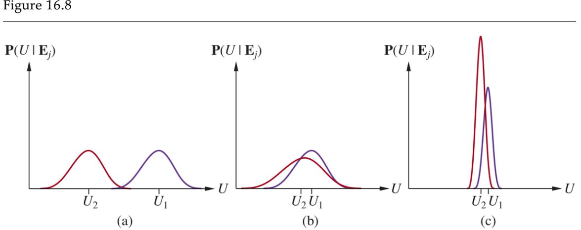
Three generic cases for the value of information. In (a), will almost certainly remain superior to , so the information is not needed. In (b), the choice is unclear and the information is crucial. In (c), the choice is unclear, but because it makes little difference, the information is less valuable. (Note: The fact that has a high peak in (c) means that its expected value is known with higher certainty than .)

Now suppose that we are choosing between two different winding dirt roads of slightly different lengths and we are carrying a seriously injured passenger. Then, even when and are quite close, the distributions of and are very broad. There is a significant possibility that the second route will turn out to be clear while the first is blocked, and in this case the difference in utilities will be very high. The VPI formula indicates that it might be worthwhile getting the satellite reports. Such a situation is shown in Figure 16.8(b) .

Finally, suppose that we are choosing between the two dirt roads in summertime, when blockage by snow is unlikely. In this case, satellite reports might show one route to be more scenic than the other because of flowering alpine meadows, or perhaps wetter because of recent rain. It is therefore quite likely that we would change our plan if we had the information. In this case, however, the difference in value between the two routes is still likely to be very small, so we will not bother to obtain the reports. This situation is shown in Figure 16.8(c) .

In sum, information has value to the extent that it is likely to cause a change of plan and to the extent that the new plan will be significantly better than the old plan.

16.6.3 Properties of the value of information

One might ask whether it is possible for information to be deleterious: can it actually have negative expected value? Intuitively, one should expect this to be impossible. After all, one could in the worst case just ignore the information and pretend that one has never received it. This is confirmed by the following theorem, which applies to any decision-theoretic agent using any decision network with possible observations :

The expected value of information is nonnegative:

\[\forall \ j \qquad VPI(E\_j) \ge 0.\]

The theorem follows directly from the definition of VPI, and we leave the proof as an exercise (Exercise 16.NNVP). It is, of course, a theorem about expected value, not actual value. Additional information can easily lead to a plan that turns out to be worse than the original plan if the information happens to be misleading. For example, a medical test that gives a false positive result may lead to unnecessary surgery; but that does not mean that the test shouldn’t be done.

It is important to remember that VPI depends on the current state of information. It can change as more information is acquired. For any given piece of evidence , the value of acquiring it can go down (e.g., if another variable strongly constrains the posterior for ) or up (e.g., if another variable provides a clue on which builds, enabling a new and better plan to be devised). Thus, VPI is not additive. That is,

\[VPI(E\_j, E\_k) \neq VPI(E\_j) + VPI(E\_k) \qquad \text{(in general)}\dots\]

VPI is, however, order-independent. That is,

\[VPI(E\_i, E\_k) = VPI(E\_i) + VPI(E\_k|E\_i) = VPI(E\_k) + VPI(E\_i|E\_k) = VPI(E\_k, E\_i)\]

where the notation denotes the VPI calculated according to the posterior distribution where is already observed. Order independence distinguishes sensing actions from ordinary actions and simplifies the problem of calculating the value of a sequence of sensing actions. We return to this question in the next section.

16.6.4 Implementation of an information-gathering agent

A sensible agent should ask questions in a reasonable order, should avoid asking questions that are irrelevant, should take into account the importance of each piece of information in relation to its cost, and should stop asking questions when that is appropriate. All of these capabilities can be achieved by using the value of information as a guide.

Figure 16.9 shows the overall design of an agent that can gather information intelligently before acting. For now, we assume that with each observable evidence variable , there is an associated cost, , which reflects the cost of obtaining the evidence through tests, consultants, questions, or whatever. The agent requests what appears to be the most efficient observation in terms of utility gain per unit cost. We assume that the result of the action is that the next percept provides the value of . If no observation is worth its cost, the agent selects a “real” action.

Figure 16.9

Design of a simple, myopic information-gathering agent. The agent works by repeatedly selecting the observation with the highest information value, until the cost of the next observation is greater than its expected benefit.

The agent algorithm we have described implements a form of information gathering that is called myopic. This is because it uses the VPI formula shortsightedly, calculating the value of information as if only a single evidence variable will be acquired. Myopic control is based on the same heuristic idea as greedy search and often works well in practice. (For example, it has been shown to outperform expert physicians in selecting diagnostic tests.) However, if there is no single evidence variable that will help a lot, a myopic agent might hastily take an action when it would have been better to request two or more variables first and then take action. The next section considers the possibility of obtaining multiple observations.

16.6.5 Nonmyopic information gathering

The fact that the value of a sequence of observations is invariant under permutations of the sequence is intriguing but doesn’t, by itself, lead to efficient algorithms for optimal information gathering. Even if we restrict ourselves to choosing in advance a fixed subset of observations to collect, there are possible such subsets from potential observations. In the general case, we face an even more complex problem of finding an optimal conditional plan (as described in Section 11.5.2 ) that chooses an observation and then acts or chooses more observations, depending on the outcome. Such plans form trees, and the number of such trees is superexponential in . 9

9 The general problem of generating sequential behavior in a partially observable environment falls under the heading of partially observable Markov decision processes, which are described in Chapter 17 .

For observations of variables in a decision network, it turns out that this problem is intractable even when the network is a polytree. There are, however, special cases in which the problem can be solved efficiently. Here we present one such case: the treasure hunt problem (or the least-cost testing sequence problem, for the less romantically inclined). There are locations ; each location contains treasure with independent probability ; and it costs to check location . This corresponds to a decision network where all the potential evidence variables are absolutely independent. The agent examines locations in some order until treasure is found; the question is, what is the optimal order?

Treasure hunt

To answer this question, we will need to consider the expected costs and success probabilities of various sequences of observations, assuming the agent stops when treasure is found. Let be such a sequence; be the concatenation of sequences and ; be

the expected cost of ; be the probability that sequence succeeds in finding treasure; and be the probability that it fails. Given these definitions, we have

(16.3)

\[C(\mathbf{x}\mathbf{y}) = C(\mathbf{x}) + F(\mathbf{x})C(\mathbf{y})\,,\]

that is, the sequence will definitely incur the cost of and, if fails, it will also incur the cost of .

The basic idea in any sequence optimization problem is to look at the change in cost, defined by , when two adjacent subsequences and in a general sequence are flipped. When the sequence is optimal, all such changes make the sequence worse. The first step is to show that the sign of the effect (increasing or decreasing the cost) doesn’t depend on the context provided by and . We have

\[\begin{aligned} \triangle &= \left[C\left(\mathbf{w}\right) + F\left(\mathbf{w}\right)C\left(\mathbf{xyz}\right)\right] - \left[C\left(\mathbf{w}\right) + F\left(\mathbf{w}\right)C\left(\mathbf{yxz}\right)\right] \quad \text{(by Equation (16.3))}\\ &= \left[F\left(\mathbf{w}\right)\left[C\left(\mathbf{xyz}\right) - C\left(\mathbf{yxz}\right)\right]\right] \\ &= \left[F\left(\mathbf{w}\right)\left[C\left(\mathbf{xy}\right) + F\left(\mathbf{xy}\right)C\left(\mathbf{z}\right)\right] - \left(C\left(\mathbf{yx}\right) + F\left(\mathbf{yx}\right)C\left(\mathbf{z}\right)\right)\right] \quad \text{(by Equation (16.3))}\\ &= \left[F\left(\mathbf{w}\right)\left[C\left(\mathbf{xy}\right) - C\left(\mathbf{yx}\right)\right] \quad \text{(since } F\left(\mathbf{xy}\right) = F\left(\mathbf{yx}\right)\text{)}. \end{aligned}\]

So we have shown that the direction of the change in the cost of the whole sequence depends only on the direction of the change in cost of the pair of elements being flipped; the context of the pair doesn’t matter. This gives us a way to sort the sequence by pairwise comparisons to obtain an optimal solution. Specifically, we now have

\[ \begin{aligned} \triangle \quad &= \, \, F\left(\mathbf{w}\right) \left[ \left( C\left(\mathbf{x}\right) + F\left(\mathbf{x}\right) C\left(\mathbf{y}\right) \right) - \left( C\left(\mathbf{y}\right) + F\left(\mathbf{y}\right) C\left(\mathbf{x}\right) \right) \right] \quad &\text{(by Equation (16.3))}\\ &= \, \, F\left(\mathbf{w}\right) \left[ C\left(\mathbf{x}\right) \left( 1 - F\left(\mathbf{y}\right) \right) - C\left(\mathbf{y}\right) \left( 1 - F\left(\mathbf{x}\right) \right) \right] = \, F\left(\mathbf{w}\right) \left[ C\left(\mathbf{x}\right) P\left(\mathbf{y}\right) - C\left(\mathbf{y}\right) P\left(\mathbf{x}\right) \right]. \end{aligned} \]

This holds for any sequences and , so it holds specifically when and are single observations of locations and , respectively. So we know that, for and to be adjacent in an optimal sequence, we must have , or . In other words, the optimal order ranks the locations according to the success probability per unit cost. Exercise 16.HUNT asks you to determine whether this is in fact the policy followed by the algorithm in Figure 16.9 for this problem.

16.6.6 Sensitivity analysis and robust decisions

The practice of sensitivity analysis is widespread in technological disciplines: it means analyzing how much the output of a process changes as the model parameters are tweaked. Sensitivity analysis in probabilistic and decision-theoretic systems is particularly important because the probabilities used are typically either learned from data or estimated by human experts, which means that they are themselves subject to considerable uncertainty. Only in rare cases, such as the dice rolls in backgammon, are the probabilities objectively known.

Sensitivity analysis

For a utility-driven decision-making process, you can think of the output as either the actual decision made or the expected utility of that decision. Consider the latter first: because expectation depends on probabilities from the model, we can compute the derivative of the expected utility of any given action with respect to each of those probability values. (For example, if all the conditional probability distributions in the model are explicitly tabulated, then computing the expectation involves computing a ratio of two sum-of-product expressions; for more on this, see Chapter 20 .) Thus, one can determine which parameters in the model have the largest effect on the expected utility of the final decision.

If, instead, we are concerned about the actual decision made, rather than its utility according to the model, then we can simply vary the parameters systematically (perhaps using binary search) to see whether the decision changes, and, if so, what is the smallest perturbation that causes such a change. One might think it doesn’t matter that much which decision is made, only what its utility is. That’s true, but in practice there may be a very substantial difference between the real utility of a decision and the utility according to the model.

If all reasonable perturbations of the parameters leave the optimal decision unchanged, then it is reasonable to assume the decision is a good one, even if the utility estimate for that decision is substantially incorrect. If, on the other hand, the optimal decision changes considerably as the parameters of the model change, then there is a good chance that the model may produce a decision that is substantially suboptimal in reality. In that case, it is worth investing further effort to refine the model.

These intuitions have been formalized in several fields (control theory, decision analysis, risk management) that propose the notion of a robust or minimax decision—that is, one that gives the best result in the worst case. Here, “worst case” means worst with respect to all plausible variations in the parameter values of the model. Letting stand for all the parameters in the model, the robust decision is defined by

\[a^\* = \underset{a}{\text{argmax}} \min\_{\theta} EU(a;\theta).\]

Robust

In many cases, particularly in control theory, the robust approach leads to designs that work very reliably in practice. In other cases, it leads to overly conservative decisions. For example, when designing a self-driving car, the robust approach would assume the worst case for the behavior of the other vehicles on the road—that is, they are all driven by homicidal maniacs. In that case, the optimal solution for the car is to stay in the garage.

Bayesian decision theory offers an alternative to robust methods: if there is uncertainty about the parameters of the model, then model that uncertainty using hyperparameters.

Whereas the robust approach might say that some probability in the model could be anywhere between 0.3 and 0.7, with the actual value chosen by an adversary to make things come out as badly as possible, the Bayesian approach would put a prior probability distribution on and then proceed as before. This requires more modeling effort—for example, the Bayesian modeler must decide if parameters and are independent—but often results in better performance in practice.

In addition to parametric uncertainty, applications of decision theory in the real world also suffer from structural uncertainty. For example, the assumption of independence of AirTraffic, Litigation, and Construction in Figure 16.6 may be incorrect, and there may be additional variables that the model simply omits. At present, we do not have a good understanding of how to take this kind of uncertainty into account. One possibility is to

keep an ensemble of models, perhaps generated by machine learning algorithms, in the hope that the ensemble captures the significant variations that matter.

16.7 Unknown Preferences

In this section we discuss what happens when there is uncertainty about the utility function whose expected value is to be optimized. There are two versions of this problem: one in which an agent (machine or human) is uncertain about its own utility function, and another in which a machine is supposed to help a human but is uncertain about what the human wants.

16.7.1 Uncertainty about one’s own preferences

Imagine that you are at an ice-cream shop in Thailand and they have only two flavors left: vanilla and durian. Both cost . You know you have a moderate liking for vanilla and you’d be willing to pay up to for a vanilla ice cream on such a hot day, so there is a net gain of for choosing vanilla. On the other hand, you have no idea whether you like durian or not, but you’ve read on Wikipedia that the durian elicits different responses from different people: some find that “it surpasses in flavour all other fruits of the world” while others liken it to “sewage, stale vomit, skunk spray and used surgical swabs.”

To put some numbers on this, let’s say there’s a 50% chance you’ll find it sublime and a 50% chance you’ll hate it ( if the taste lingers all afternoon). Here, there’s no uncertainty about what prize you’re going to win—it’s the same durian ice cream either way —but there’s uncertainty about your own preferences for that prize.

We could extend the decision network formalism to allow for uncertain utilities, as shown in Figure 16.10(a) . If there is no more information to be obtained about your durian preferences, however—for example, if the shop won’t let you taste it first—then the decision problem is identical to the one shown in Figure 16.10(b) . We can simply replace the uncertain value of the durian with its expected net gain of and your decision will remain unchanged.

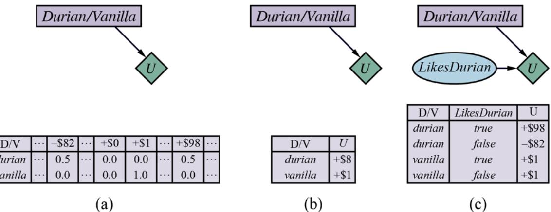
1. A decision network for the ice cream choice with an uncertain utility function. (b) The network with the expected utility of each action. (c) Moving the uncertainty from the utility function into a new random variable.

If it’s possible for your beliefs about durian to change—perhaps you get a tiny taste, or you find out that all of your living relatives love durian—then the transformation in Figure 16.10(b) is not valid. It turns out, however, that we can still find an equivalent model in which the utility function is deterministic. Rather than saying there is uncertainty about the utility function, we move that uncertainty “into the world,” so to speak. That is, we create a new random variable LikesDurian with prior probabilities of 0.5 for true and false, as shown in Figure 16.10(c) . With this extra variable, the utility function becomes deterministic, but we can still handle changing beliefs about your durian preferences.

The fact that unknown preferences can be modeled by ordinary random variables means that we can keep using the machinery and theorems developed for known preferences. On the other hand, it doesn’t mean that we can always assume that preferences are known. The uncertainty is still there and still affects how agents should behave.

16.7.2 Deference to humans

Now let’s turn to the second case mentioned above: a machine that is supposed to help a human but is uncertain about what the human wants. The full treatment of this case must be deferred to Chapter 18 , where we discuss decisions involving more than one agent. Here, we ask one simple question: under what circumstances will such a machine defer to the human?

To study this question, let’s consider a very simple scenario, as shown in Figure 16.11 . Robbie is a software robot working for Harriet, a busy human, as her personal assistant. Harriet needs a hotel room for her next business meeting in Geneva. Robbie can act now let’s say he can book Harriet into a very expensive hotel near the meeting venue. He is quite unsure how much Harriet will like the hotel and its price; let’s say he has a uniform probability for its net value to Harriet between and , with an average of . He could also “switch himself off”—less melodramatically, take himself out of the hotel booking process altogether—which we define (without loss of generality) to have value to Harriet. If those were his two choices, he would go ahead and book the hotel, incurring a significant risk of making Harriet unhappy. (If the range were to , with average , he would switch himself off instead.) We’ll give Robbie a third choice, however: explain his plan, wait, and let Harriet switch him off. Harriet can either switch him off or let him go ahead and book the hotel. What possible good could this do, one might ask, given that he could make both of those choices himself?

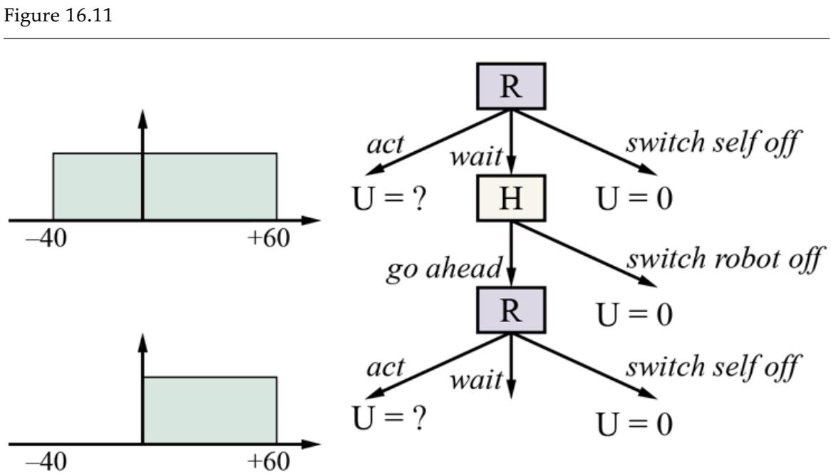
The off-switch game. , the robot, can choose to act now, with a highly uncertain payoff; to switch itself off; or to defer to , the human. can switch off or let it go ahead. now has the same choice again. Acting still has an uncertain payoff, but now knows the payoff is nonnegative.

The point is that Harriet’s choice—to switch Robbie off or let him go ahead—provides Robbie with information about Harriet’s preferences. We’ll assume, for now, that Harriet is rational, so if Harriet lets Robbie go ahead, it means the value to Harriet is positive. Now, as shown in Figure 16.11 , Robbie’s belief changes: it is uniform between and , with an average of .

So, if we evaluate Robbie’s initial choices from his point of view:

• 1. Acting now and booking the hotel has an expected value of .
• 2. Switching himself off has a value of .
• 3. Waiting and letting Harriet switch him off leads to two possible outcomes:
  • a. There is a 40% chance, based on Robbie’s uncertainty about Harriet’s preferences, that she will hate the plan and will switch Robbie off, with value .
  • b. There is a 60% chance Harriet will like the plan and allow Robbie to go ahead, with expected value .

Thus, waiting has expected value , which is better than the Robbie epects if he acts now.

The upshot is that Robbie has a positive incentive to defer to Harriet—that is, to allow himself to be switched off. This incentive comes directly from Robbie’s uncertainty about Harriet’s preferences. Robbie is aware that there’s a chance (40% in this example) that he might be about to do something that will make Harriet unhappy, in which case being switched off would be preferable to going ahead. Were Robbie already certain about Harriet’s preferences, he would just go ahead and make the decision (or switch himself off); there would be absolutely nothing to be gained from consulting Harriet, because, according to Robbie’s definite beliefs, he can already predict exactly what she is going to decide.

In fact, it is possible to prove the same result in the general case: as long as Robbie is not completely certain that he’s about to do what Harriet herself would do, he is better off allowing her to switch him off. Intuitively, her decision provides Robbie with information, and the expected value of information is always nonnegative. Conversely, if Robbie is certain about Harriet’s decision, her decision provides no new information, and so Robbie has no incentive to allow her to decide.

Formally, let be Robbie’s prior probability density over Harriet’s utility for the proposed action . Then the value of going ahead with is

\[EU(a) = \int\_{-\infty}^{\infty} P(u) \cdot u \, du = \int\_{-\infty}^{0} P(u) \cdot u \, du + \int\_{0}^{\infty} P(u) \cdot u \, du.\]

(We will see shortly why the integral is split up in this way.) On the other hand, the value of action , deferring to Harriet, is composed of two parts: if then Harriet lets Robbie go ahead, so the value is , but if then Harriet switches Robbie off, so the value is 0:

\[EU(d) = \int\_{-\infty}^{0} P(u) \cdot 0 \, du + \int\_{0}^{\infty} P(u) \cdot u \, du.\]

Comparing the expressions for and , we see immediately that

\[EU(d) \ge EU(a)\]

because the expression for has the negative-utility region zeroed out. The two choices have equal value only when the negative region has zero probability—that is, when Robbie is already certain that Harriet likes the proposed action.

There are some obvious elaborations on the model that are worth exploring immediately. The first elaboration is to impose a cost for Harriet’s time. In that case, Robbie is less inclined to bother Harriet if the downside risk is small. This is as it should be. And if Harriet is really grumpy about being interrupted, she shouldn’t be too surprised if Robbie occasionally does things she doesn’t like.

The second elaboration is to allow for some probability of human error—that is, Harriet might sometimes switch Robbie off even when his proposed action is reasonable, and she might sometimes let Robbie go ahead even when his proposed action is undesirable. It is straightforward to fold this error probability into the model (see Exercise 16.OFFS). As one might expect, the solution shows that Robbie is less inclined to defer to an irrational Harriet who sometimes acts against her own best interests. The more randomly she behaves, the more uncertain Robbie has to be about her preferences before deferring to her. Again, this is as it should be: for example, if Robbie is a self-driving car and Harriet is his naughty twoyear-old passenger, Robbie should not allow Harriet to switch him off in the middle of the highway.

Summary

This chapter shows how to combine utility theory with probability to enable an agent to select actions that will maximize its expected performance.

• Probability theory describes what an agent should believe on the basis of evidence, utility theory describes what an agent wants, and decision theory puts the two together to describe what an agent should do.
• We can use decision theory to build a system that makes decisions by considering all possible actions and choosing the one that leads to the best expected outcome. Such a system is known as a rational agent.
• Utility theory shows that an agent whose preferences between lotteries are consistent with a set of simple axioms can be described as possessing a utility function; furthermore, the agent selects actions as if maximizing its expected utility.
• Multiattribute utility theory deals with utilities that depend on several distinct attributes of states. Stochastic dominance is a particularly useful technique for making unambiguous decisions, even without precise utility values for attributes.
• Decision networks provide a simple formalism for expressing and solving decision problems. They are a natural extension of Bayesian networks, containing decision and utility nodes in addition to chance nodes.
• Sometimes, solving a problem involves finding more information before making a decision. The value of information is defined as the expected improvement in utility compared with making a decision without the information; it is particularly useful for guiding the process of information-gathering prior to making a final decision.
• When, as is often the case, it is impossible to specify the human’s utility function completely and correctly, machines must operate under uncertainty about the true objective. This makes a significant difference when the possibility exists for the machine to acquire more information about human preferences. We showed by a simple argument that uncertainty about preferences ensures that the machine defers to the human, to the point of allowing itself to be switched off.

Bibliographical and Historical Notes

In the 17th century treatise L’art de Penser, or Port-Royal Logic, Arnauld (1662) states:

To judge what one must do to obtain a good or avoid an evil, it is necessary to consider not only the good and the evil in itself, but also the probability that it happens or does not happen; and to view geometrically the proportion that all these things have together.

Modern texts talk of utility rather than good and evil, but this statement correctly notes that one should multiply utility by probability (“view geometrically”) to give expected utility, and maximize that over all outcomes (“all these things”) to “judge what one must do.” It is remarkable how much Arnauld got right, more than 350 years ago, and only 8 years after Pascal and Fermat first showed how to use probability correctly.

Daniel Bernoulli (1738), investigating the St. Petersburg paradox (see Exercise 16.STPT), was the first to realize the importance of preference measurement for lotteries, writing “the value of an item must not be based on its price, but rather on the utility that it yields” (italics his). Utilitarian philosopher Jeremy Bentham (1823) proposed the hedonic calculus for weighing “pleasures” and “pains,” arguing that all decisions (not just monetary ones) could be reduced to utility comparisons.

Hedonic calculus

Bernoulli’s introduction of utility—an internal, subjective quantity—to explain human behavior via a mathematical theory was an utterly remarkable proposal for its time. It was all the more remarkable for the fact that unlike monetary amounts, the utility values of various bets and prizes are not directly observable; instead, utilities are to be inferred from the preferences exhibited by an individual. It would be two centuries before the implications of the idea were fully worked out and it became broadly accepted by statisticians and economists.

The derivation of numerical utilities from preferences was first carried out by Ramsey (1931); the axioms for preference in the present text are closer in form to those rediscovered in Theory of Games and Economic Behavior (von Neumann and Morgenstern, 1944). Ramsey had derived subjective probabilities (not just utilities) from an agent’s preferences; Savage (1954) and Jeffrey (1983) carry out more recent constructions of this kind. Beardon et al. (2002) show that a utility function does not suffice to represent nontransitive preferences and other anomalous situations.

In the post-war period, decision theory became a standard tool in economics, finance, and management science. A field of decision analysis emerged to aid in making policy decisions more rational in areas such as military strategy, medical diagnosis, public health, engineering design, and resource management. The process involves a decision maker who states preferences between outcomes and a decision analyst who enumerates the possible actions and outcomes and elicits preferences from the decision maker to determine the best course of action. Von Winterfeldt and Edwards (1986) provide a nuanced perspective on decision analysis and its relationship to human preference structures. Smith (1988) gives an overview of the methodology of decision analysis.

Decision analysis

Decision maker

Decision analyst

Until the 1980s, multivariate decision problems were handled by constructing “decision trees” of all possible instantiations of the variables. Influence diagrams or decision networks, which take advantage of the same conditional independence properties as Bayesian networks, were introduced by Howard and Matheson (1984), based on earlier work at SRI

(Miller et al., 1976). Howard and Matheson’s algorithm constructed the complete (exponentially large) decision tree from the decision network. Shachter (1986) developed a method for making decisions based directly on a decision network, without the creation of an intermediate decision tree. This algorithm was also one of the first to provide complete inference for multiply connected Bayesian networks. Nilsson and Lauritzen (2000) link algorithms for decision networks to ongoing developments in clustering algorithms for Bayesian networks. The collection by Oliver and Smith (1990) has a number of useful early articles on decision networks, as does the 1990 special issue of the journal Networks. The text by Fenton and Neil (2018) provides a hands-on guide to solving real-world decision problems using decision networks. Papers on decision networks and utility modeling also appear regularly in the journals Management Science and Decision Analysis.

Surprisingly few early AI researchers adopted decision-theoretic tools after the early applications in medical decision making described in Chapter 12 . One of the few exceptions was Jerry Feldman, who applied decision theory to problems in vision (Feldman and Yakimovsky, 1974) and planning (Feldman and Sproull, 1977). Rule-based expert systems of the late 1970s and early 1980s concentrated on answering questions, rather than on making decisions. Those systems that did recommend actions generally did so using condition–action rules rather than explicit representations of outcomes and preferences.

Decision networks offer a far more flexible approach, for example by allowing preferences to change while keeping the transition model constant, or vice versa. They also allow a principled calculation of what information to seek next. In the late 1980s, partly due to Pearl’s work on Bayes nets, decision-theoretic expert systems gained widespread acceptance (Horvitz et al., 1988; Cowell et al., 2002). In fact, from 1991 onward, the cover design of the journal Artificial Intelligence has depicted a decision network, although some artistic license appears to have been taken with the direction of the arrows.

Practical attempts to measure human utilities began with post-war decision analysis (see above). The micromort utility measure is discussed by Howard (1989). Thaler Thaler (1992) found that for a chance of death, a respondent wouldn’t pay more than to remove the risk, but wouldn’t accept to take on the risk.

The use of QALYs (quality-adjusted life years) to perform cost–benefit analyses of medical interventions and related social policies dates back at least to work by Klarman et al. (1968), although the term itself was first used by Zeckhauser and Shepard (1976). Like money, QALYs correspond directly to utilities only under fairly strong assumptions, such as risk neutrality, that are often violated (Beresniak et al., 2015); nonetheless, QALYs are much widely used in practice, for example in forming National Health Service policies in the UK. See Russell (1990) for a typical example of an argument for a major change in public health policy on grounds of increased expected utility measured in QALYs.

Keeney and Raiffa (1976) give an introduction to multiattribute utility theory. They describe early computer implementations of methods for eliciting the necessary parameters for a multiattribute utility function and include extensive accounts of real applications of the theory. Abbas (2018) covers many advances since 1976. The theory was introduced to AI primarily by the work of Wellman (1985), who also investigated the use of stochastic dominance and qualitative probability models (Wellman, 1988; 1990a). Wellman and Doyle (1992) provide a preliminary sketch of how a complex set of utility-independence relationships might be used to provide a structured model of a utility function, in much the same way that Bayesian networks provide a structured model of joint probability distributions. Bacchus and Grove (1995, 1996) and La Mura and Shoham (1999) give further results along these lines. Boutilier et al. (2004) describe CP-nets, a fully worked out graphical model formalism for conditional ceteribus paribus preference statements.

The optimizer’s curse was brought to the attention of decision analysts in a forceful way by Smith and Winkler (2006), who pointed out that the financial benefits to the client projected by analysts for their proposed course of action almost never materialized. They trace this directly to the bias introduced by selecting an optimal action and show that a more complete Bayesian analysis eliminates the problem.

Post-decision disappointment

Winner’s curse

The same underlying concept has been called post-decision disappointment by Harrison and March (1984) and was noted in the context of analyzing capital investment projects by Brown (1974). The optimizer’s curse is also closely related to the winner’s curse (Capen et al., 1971; Thaler, 1992), which applies to competitive bidding in auctions: whoever wins the auction is very likely to have overestimated the value of the object in question. Capen et al. quote a petroleum engineer on the topic of bidding for oil-drilling rights: “If one wins a tract against two or three others he may feel fine about his good fortune. But how should he feel if he won against 50 others? Ill.”

The Allais paradox, due to Nobel Prize–winning economist Maurice Allais (1953), was tested experimentally to show that people are consistently inconsistent in their judgments (Tversky and Kahneman, 1982; Conlisk, 1989). The Ellsberg paradox on ambiguity aversion was introduced in the Ph.D. thesis of Daniel Ellsberg, (1962). Fox and Tversky (1995) describe a further study of ambiguity aversion. Machina (2005) gives an overview of choice under uncertainty and how it can vary from expected utility theory. See the classic text by Keeney and Raiffa (1976) and the more recent work by Abbas (2018) for an in-depth analysis of preferences with uncertainty. 10

10 Ellsberg later became a military analyst at the RAND Corporation and leaked documents known as the Pentagon Papers, thereby contributing to the end of the Vietnam war.

2009 was a big year for popular books on human irrationality, including Predictably Irrational (Ariely, 2009), Sway (Brafman and Brafman, 2009), Nudge (Thaler and Sunstein, 2009), Kluge (Marcus, 2009), How We Decide (Lehrer, 2009) and On Being Certain (Burton, 2009). They complement the classic book Judgment Under Uncertainty (Kahneman et al., 1982) and the article that started it all (Kahneman and Tversky, 1979). Kahneman himself provides an insightful and readable account in Thinking: Fast and Slow (Kahneman, 2011).

Irrationality

The field of evolutionary psychology (Buss, 2005), on the other hand, has run counter to this literature, arguing that humans are quite rational in evolutionarily appropriate contexts. Its adherents point out that irrationality is penalized by definition in an evolutionary context

and show that in some cases it is an artifact of the experimental setup (Cummins and Allen, 1998). There has been a recent resurgence of interest in Bayesian models of cognition, overturning decades of pessimism (Elio, 2002; Chater and Oaksford, 2008; Griffiths et al., 2008); this resurgence is not without its detractors, however (Jones and Love, 2011).

The theory of information value was explored first in the context of statistical experiments, where a quasi-utility (entropy reduction) was used (Lindley, 1956). The control theorist Ruslan Stratonovich (1965) developed the more general theory presented here, in which information has value by virtue of its ability to affect decisions. Stratonovich’s work was not known in the West, where Ron Howard (1966) pioneered the same idea. His paper ends with the remark “If information value theory and associated decision theoretic structures do not in the future occupy a large part of the education of engineers, then the engineering profession will find that its traditional role of managing scientific and economic resources for the benefit of man has been forfeited to another profession.” To date, the implied revolution in managerial methods has not occurred.

The myopic information-gathering algorithm described in the chapter is ubiquitous in the decision analysis literature; its basic outlines can be discerned in the original paper on influence diagrams (Howard and Matheson, 1984). Efficient calculation methods are studied by Dittmer and Jensen (1997). Laskey (1995) and Nielsen and Jensen (2003) discuss methods for sensitivity analysis in Bayesian networks and decision networks, respectively. The classic text Robust and Optimal Control (Zhou et al., 1995) provides thorough coverage and comparison of the robust and decision-theoretic approaches to decisions under uncertainty.

The treasure hunt problem was solved independently by many authors, dating back at least to papers on sequential testing by Gluss (1959) and Mitten (1960). The style of proof in this chapter draws on a basic result, due to Smith (1956), relating the value of a sequence to the value of the same sequence with two adjacent elements permuted. These results for independent tests were extended to more general tree and graph search problems (where the tests are partially ordered) by Kadane and Simon (1977). Results on the complexity of non-myopic calculations of the value of information were obtained by Krause and Guestrin (2009). Krause et al. (2008) identified cases where submodularity leads to a tractable approximation algorithm, drawing on the seminal work of Nemhauser et al. (1978) on submodular functions; Krause and Guestrin (2005) identify cases where an exact dynamic

programming algorithm gives an efficient solution for both evidence subset election and conditional plan generation.

Harsanyi (1967) studied the problem of incomplete information in game theory, where players may not know each others’ payoff functions exactly. He showed that such games were identical to games with imperfect information, where players are uncertain about the state of the world, via the trick of adding state variables referring to players’ payoffs. Cyert and de Groot (1979) developed a theory of adaptive utility in which an agent could be uncertain about its own utility function and could obtain more information through experience.

Adaptive utility

Work on Bayesian preference elicitation (Chajewska et al., 2000; Boutilier, 2002) begins from the assumption of a prior probability over the agent’s utility function. Fern et al. (2014) propose a decision-theoretic model of assistance in which a robot tries to ascertain and assist with a human goal about which it is initially uncertain. The off-switch example in Section 16.7.2 is adapted from Hadfield-Menell et al. (2017b). Russell (2019) proposes a general framework for benefical AI in which the off-switch game is a key example.

Assistance

Chapter 17 Making Complex Decisions

In which we examine methods for deciding what to do today, given that we may face another decision tomorrow.

In this chapter, we address the computational issues involved in making decisions in a stochastic environment. Whereas Chapter 16 was concerned with one-shot or episodic decision problems, in which the utility of each action’s outcome was well known, we are concerned here with sequential decision problems, in which the agent’s utility depends on a sequence of decisions. Sequential decision problems incorporate utilities, uncertainty, and sensing, and include search and planning problems as special cases. Section 17.1 explains how sequential decision problems are defined, and Section 17.2 describes methods for solving them to produce behaviors that are appropriate for a stochastic environment. Section 17.3 covers multi-armed bandit problems, a specific and fascinating class of sequential decision problems that arise in many contexts. Section 17.4 explores decision problems in partially observable environments and Section 17.5 describes how to solve them.

Sequential decision problem

17.1 Sequential Decision Problems

Suppose that an agent is situated in the environment shown in Figure 17.1(a) . Beginning in the start state, it must choose an action at each time step. The interaction with the environment terminates when the agent reaches one of the goal states, marked or . Just as for search problems, the actions available to the agent in each state are given by ACTIONS(s), sometimes abbreviated to ; in the environment, the actions in every state are Up, Down, Left, and Right. We assume for now that the environment is fully observable, so that the agent always knows where it is.

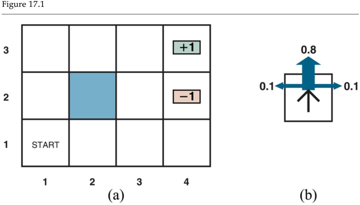
1. A simple, stochastic environment that presents the agent with a sequential decision problem. (b) Illustration of the transition model of the environment: the “intended” outcome occurs with probability 0.8, but with probability 0.2 the agent moves at right angles to the intended direction. A collision with a wall results in no movement. Transitions into the two terminal states have reward and , respectively, and all other transitions have a reward of .

If the environment were deterministic, a solution would be easy: [Up, Up, Right, Right, Right]. Unfortunately, the environment won’t always go along with this solution, because the actions are unreliable. The particular model of stochastic motion that we adopt is illustrated in Figure 17.1(b) . Each action achieves the intended effect with probability 0.8, but the rest of the time, the action moves the agent at right angles to the intended direction.

Furthermore, if the agent bumps into a wall, it stays in the same square. For example, from the start square (1,1), the action Up moves the agent to (1,2) with probability 0.8, but with probability 0.1, it moves right to (2,1), and with probability 0.1, it moves left, bumps into the wall, and stays in (1,1). In such an environment, the sequence [Up,Up,Right,Right,Right] goes up around the barrier and reaches the goal state at (4,3) with probability . There is also a small chance of accidentally reaching the goal by going the other way around with probability , for a grand total of 0.32776. (See also Exercise 17.MDPX.)

As in Chapter 3 , the transition model (or just “model,” when the meaning is clear) describes the outcome of each action in each state. Here, the outcome is stochastic, so we write for the probability of reaching state if action is done in state . (Some authors write for the transition model.) We will assume that transitions are Markovian: the probability of reaching from depends only on and not on the history of earlier states.

To complete the definition of the task environment, we must specify the utility function for the agent. Because the decision problem is sequential, the utility function will depend on a sequence of states and actions—an environment history—rather than on a single state. Later in this section, we investigate the nature of utility functions on histories; for now, we simply stipulate that for every transition from to via action , the agent receives a reward . The rewards may be positive or negative, but they are bounded by . 1

1 It is also possible to use costs , as we did in the definition of search problems in Chapter 3 . The use of rewards is, however, standard in the literature on sequential decisions under uncertainty.

Reward

For our particular example, the reward is for all transitions except those entering terminal states (which have rewards and ). The utility of an environment history is just (for now) the sum of the rewards received. For example, if the agent reaches the state after 10 steps, its total utility will be . The negative reward of gives the agent an incentive to reach (4,3) quickly, so our environment is a stochastic generalization of the search problems of Chapter 3 . Another way of saying this is that the agent does not enjoy living in this environment and so it wants to leave as soon as possible.

To sum up: a sequential decision problem for a fully observable, stochastic environment with a Markovian transition model and additive rewards is called a Markov decision process, or MDP, and consists of a set of states (with an initial state ); a set ACTIONS(s) of actions in each state; a transition model ; and a reward function . Methods for solving MDPs usually involve dynamic programming: simplifying a problem by recursively breaking it into smaller pieces and remembering the optimal solutions to the pieces.

Markov decision process

Dynamic programming

The next question is, what does a solution to the problem look like? No fixed action sequence can solve the problem, because the agent might end up in a state other than the goal. Therefore, a solution must specify what the agent should do for any state that the agent might reach. A solution of this kind is called a policy. It is traditional to denote a policy by , and is the action recommended by the policy for state . No matter what the outcome of the action, the resulting state will be in the policy, and the agent will know what to do next.

Policy

Each time a given policy is executed starting from the initial state, the stochastic nature of the environment may lead to a different environment history. The quality of a policy is

therefore measured by the expected utility of the possible environment histories generated by that policy. An optimal policy is a policy that yields the highest expected utility. We use to denote an optimal policy. Given , the agent decides what to do by consulting its current percept, which tells it the current state , and then executing the action . A policy represents the agent function explicitly and is therefore a description of a simple reflex agent, computed from the information used for a utility-based agent.

Optimal policy

The optimal policies for the world of Figure 17.1 are shown in Figure 17.2(a) . There are two policies because the agent is exactly indifferent between going left and going up from (3,1): going left is safer but longer, while going up is quicker but risks falling into (4,2) by accident. In general there will often be multiple optimal policies.

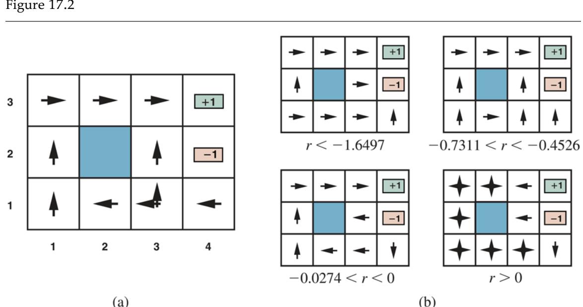
1. The optimal policies for the stochastic environment with for transitions between nonterminal states. There are two policies because in state (3,1) both Left and Up are optimal. (b) Optimal policies for four different ranges of .

The balance of risk and reward changes depending on the value of for transitions between nonterminal states. The policies shown in Figure 17.2(a) are optimal for . Figure 17.2(b) shows optimal policies for four other ranges of . When , life is so painful that the agent heads straight for the nearest exit, even if the exit is worth . When , life is quite unpleasant; the agent takes the shortest route to the state from (2,1), (3,1), and (3,2), but from (4,1) the cost of reaching is so high that the agent prefers to dive straight into . When life is only slightly dreary ( ), the optimal policy takes no risks at all. In (4,1) and (3,2), the agent heads directly away from the state so that it cannot fall in by accident, even though this means banging its head against the wall quite a few times. Finally, if , then life is positively enjoyable and the agent avoids both exits. As long as the actions in (4,1), (3,2), and (3,3) are as shown, every policy is optimal, and the agent obtains infinite total reward because it never enters a terminal state. It turns out that there are nine optimal policies in all for various ranges of ; Exercise 17.THRC asks you to find them.

The introduction of uncertainty brings MDPs closer to the real world than deterministic search problems. For this reason, MDPs have been studied in several fields, including AI, operations research, economics, and control theory. Dozens of solution algorithms have been proposed, several of which we discuss in Section 17.2 . First, however, we spell out in more detail the definitions of utilities, optimal policies, and models for MDPs.

17.1.1 Utilities over time

In the MDP example in Figure 17.1 , the performance of the agent was measured by a sum of rewards for the transitions experienced. This choice of performance measure is not arbitrary, but it is not the only possibility for the utility function on environment histories, which we write as . 2

2 In this chapter we use for the utility function (to be consistent with the rest of the book), but many works about MDPs use (for value) instead.

The first question to answer is whether there is a finite horizon or an infinite horizon for decision making. A finite horizon means that there is a fixed time after which nothing matters—the game is over, so to speak. Thus,

\[U\_h([s\_0, a\_0, s\_1, a\_1, \dots, s\_{N+k}]) = U\_h([s\_0, a\_0, s\_1, a\_1, \dots, s\_N])\]

Finite horizon

Infinite horizon

for all . For example, suppose an agent starts at (3,1) in the world of Figure 17.1 , and suppose that . Then, to have any chance of reaching the state, the agent must head directly for it, and the optimal action is to go Up. On the other hand, if , then there is plenty of time to take the safe route by going Left. So, with a finite horizon, an optimal action in a given state may depend on how much time is left. A policy that depends on the time is called nonstationary.

Nonstationary policy

With no fixed time limit, on the other hand, there is no reason to behave differently in the same state at different times. Hence, an optimal action depends only on the current state, and the optimal policy is stationary. Policies for the infinite-horizon case are therefore simpler than those for the finite-horizon case, and we deal mainly with the infinite-horizon case in this chapter. (We will see later that for partially observable environments, the infinite-horizon case is not so simple.) Note that “infinite horizon” does not necessarily mean that all state sequences are infinite; it just means that there is no fixed deadline. There can be finite state sequences in an infinite-horizon MDP that contains a terminal state.

Stationary policy

The next question we must decide is how to calculate the utility of state sequences. Throughout this chapter, we will additive discounted rewards: the utility of a history is

Additive discounted reward

Discount factor

where the discount factor is a number between 0 and 1. The discount factor describes the preference of an agent for current rewards over future rewards. When is close to 0, rewards in the distant future are viewed as insignificant. When is close to 1, an agent is more willing to wait for long-term rewards. When is exactly 1, discounted rewards reduce to the special case of purely additive rewards. Notice that additivity was used implicitly in our use of path cost functions in heuristic search algorithms (Chapter 3 ).

Additive reward

There are several reasons why additive discounted rewards make sense. One is empirical: both humans and animals appear to value near-term rewards more highly than rewards in the distant future. Another is economic: if the rewards are monetary, then it really is better to get them sooner rather than later because early rewards can be invested and produce returns while you’re waiting for the later rewards. In this context, a discount factor of is equivalent to an interest rate of . For example, a discount factor of is equivalent to an interest rate of 11.1%.

A third reason is uncertainty about the true rewards: they may never arrive for all sorts of reasons that are not taken into account in the transition model. Under certain assumptions, a discount factor of gamma is equivalent to adding a probability of accidental termination at every time step, independent of the action taken.

A fourth justification arises from a natural property of preferences over histories. In the terminology of multiattribute utility theory (see Section 16.4 ), each transition can be viewed as an attribute of the history . In principle, the utility function could depend in arbitrarily complex ways on these attributes. There is, however, a highly plausible preference-independence assumption that can be made, namely that the agent’s preferences between state sequences are stationary.

Stationary preference

Assume two histories and begin with the same transition (i.e., and ). Then stationarity for preferences means that the two histories should be preference-ordered the same way as the histories and . In English, this means that if you prefer one future to another starting tomorrow, then you should still prefer that future if it were to start today instead. Stationarity is a fairly innocuous-looking assumption, but additive discounting is the only form of utility on histories that satisfies it.

A final justification for discounted rewards is that it conveniently makes some nasty infinities go away. With infinite horizons there is a potential difficulty: if the environment does not contain a terminal state, or if the agent never reaches one, then all environment histories will be infinitely long, and utilities with additive undiscounted rewards will generally be infinite. While we can agree that is better than , comparing two state sequences with utility is more difficult. There are three solutions, two of which we have seen already:

1. With discounted rewards, the utility of an infinite sequence is finite. In fact, if and rewards are bounded by , we have (17.1)

\[U\_h([s\_0, a\_0, s\_1, \dots]) = \sum\_{t=0}^{\infty} \gamma^t R(s\_t, a\_t, s\_{t+1}) \le \sum\_{t=0}^{\infty} \gamma^t R\_{\max} = \frac{R\_{\max}}{1 - \gamma},\]

using the standard formula for the sum of an infinite geometric series.

Proper policy

• 2. If the environment contains terminal states and if the agent is guaranteed to get to one eventually, then we will never need to compare infinite sequences. A policy that is guaranteed to reach a terminal state is called a proper policy. With proper policies, we can use (i.e., additive undiscounted rewards). The first three policies shown in Figure 17.2(b) are proper, but the fourth is improper. It gains infinite total reward by staying away from the terminal states when the reward for transitions between nonterminal states is positive. The existence of improper policies can cause the standard algorithms for solving MDPs to fail with additive rewards, and so provides a good reason for using discounted rewards.
• 3. Infinite sequences can be compared in terms of the average reward obtained per time step. Suppose that transitions to square (1,1) in the world have a reward of 0.1 while transitions to other nonterminal states have a reward of 0.01. Then a policy that does its best to stay in (1,1) will have higher average reward than one that stays elsewhere. Average reward is a useful criterion for some problems, but the analysis of average-reward algorithms is complex.

Average reward

Additive discounted rewards present the fewest difficulties in evaluating histories, so we shall use them henceforth.

17.1.2 Optimal policies and the utilities of states

Having decided that the utility of a given history is the sum of discounted rewards, we can compare policies by comparing the expected utilities obtained when executing them. We assume the agent is in some initial state and define (a random variable) to be the state the agent reaches at time when executing a particular policy . (Obviously, , the state the agent is in now.) The probability distribution over state sequences is determined by the initial state , the policy , and the transition model for the environment. The expected utility obtained by executing starting in is given by

(17.2)

\[U^{\pi}(s) = E\left[\sum\_{t=0}^{\infty} \gamma^t R(S\_t, \pi(S\_t), S\_{t+1})\right],\]

where the expectation is with respect to the probability distribution over state sequences determined by and . Now, out of all the policies the agent could choose to execute starting in , one (or more) will have higher expected utilities than all the others. We’ll use to denote one of these policies:

(17.3)

\[ \pi\_s^\* = \operatorname\*{argmax}\_s U^\pi(s). \]

Remember that is a policy, so it recommends an action for every state; its connection with in particular is that it’s an optimal policy when is the starting state. A remarkable consequence of using discounted utilities with infinite horizons is that the optimal policy is independent of the starting state. (Of course, the action sequence won’t be independent; remember that a policy is a function specifying an action for each state.) This fact seems intuitively obvious: if policy is optimal starting in and policy is optimal starting in , then, when they reach a third state , there’s no good reason for them to disagree with each other, or with , about what to do next. So we can simply write for an optimal policy. 3

3 Although this seems obvious, it does not hold for finite-horizon policies or for other ways of combining rewards over time, such as taking the max. The proof follows directly from the uniqueness of the utility function on states, as shown in Section 17.2.1 .

Given this definition, the true utility of a state is just —that is, the expected sum of discounted rewards if the agent executes an optimal policy. We write this as , matching the notation used in Chapter 16 for the utility of an outcome. Figure 17.3 shows the utilities for the world. Notice that the utilities are higher for states closer to the exit, because fewer steps are required to reach the exit.

Figure 17.3

3	0.8516	0.9078	0.9578	+1
2	0.8016		0.7003	l
1	0.7453	0.6953	0.6514	0.4279
	1	ର	0	ব

The utilities of the states in the world with and for transitions to nonterminal states.

The utility function allows the agent to select actions by using the principle of maximum expected utility from Chapter 16 —that is, choose the action that maximizes the reward for the next step plus the expected discounted utility of the subsequent state:

(17.4)

\[\pi^\*(s) = \operatorname\*{argmax}\_{a \in A(s)} \sum\_{s'} P(s'|s, a) [R(s, a, s') + \gamma U(s')].\]

We have defined the utility of a state, , as the expected sum of discounted rewards from that point onwards. From this, it follows that there is a direct relationship between the utility of a state and the utility of its neighbors: the utility of a state is the expected reward for the next transition plus the discounted utility of the next state, assuming that the agent chooses the optimal action. That is, the utility of a state is given by

\[U(s) = \max\_{a \in A(s)} \sum\_{s'} P(s'|s, a) [R(s, a, s') + \gamma U(s')].\]

This is called the Bellman equation, after Richard Bellman (1957). The utilities of the states —defined by Equation (17.2) as the expected utility of subsequent state sequences—are solutions of the set of Bellman equations. In fact, they are the unique solutions, as we show in Section 17.2.1 .

Bellman equation

Let us look at one of the Bellman equations for the world. The expression for is

\[\begin{aligned} \max \{ & \left[ 0.8(-0.04 + \gamma U(1, 2)) + 0.1(-0.04 + \gamma U(2, 1)) + 0.1(-0.04 + \gamma U(1, 1)) \right], \\ & \left[ 0.9(-0.04 + \gamma U(1, 1)) + 0.1(-0.04 + \gamma U(1, 2)) \right], \\ & \left[ 0.9(-0.04 + \gamma U(1, 1)) + 0.1(-0.04 + \gamma U(2, 1)) \right], \\ & \left[ 0.8(-0.04 + \gamma U(2, 1)) + 0.1(-0.04 + \gamma U(1, 2)) + 0.1(-0.04 + \gamma U(1, 1)) \right] \end{aligned}\]

where the four expressions correspond to Up, Left, Down and Right moves. When we plug in the numbers from Figure 17.3 , with , we find that Up is the best action.

Another important quantity is the action-utility function, or Q-function: is the expected utility of taking a given action in a given state. The Q-function is related to utilities in the obvious way:

(17.6)

\[U(s) = \max\_{a} Q(s, a).\]

Q-function

Furthermore, the optimal policy can be extracted from the Q-function as follows:

(17.7)

\[ \pi^\*(s) = \underset{a}{\text{argmax}} \, Q(s, a). \]

We can also develop a Bellman equation for Q-functions, noting that the expected total reward for taking an action is its immediate reward plus the discounted utility of the outcome state, which in turn can be expressed in terms of the Q-function:

(17.8)

\[\begin{aligned} Q(s,a) &= \sum\_{s'} P(s'|s,a)[R(s,a,s') + \gamma \, U(s')]\\ &= \sum\_{s'} P(s'|s,a)[R(s,a,s') + \gamma \, \max\_{a'} Q(s',a')] \end{aligned}\]

Solving the Bellman equations for (or for ) gives us what we need to find an optimal policy. The Q-function shows up again and again in algorithms for solving MDPs, so we shall use the following definition:

\[\begin{aligned} \textbf{function Q-VALUE} & \begin{pmatrix} mdp, \, s, \, a, \, U \right\rangle \textbf{ returns a utility value} \\ \textbf{return } \sum\_{s'} P\left(s'|s, \, a\right) \left[ R\left(s, \, a, \, s'\right) + \gamma U\left[s'\right] \right] \end{aligned} \]

17.1.3 Reward scales

Chapter 16 noted that the scale of utilities is arbitrary: an affine transformation leaves the optimal decision unchanged. We can replace by where and are any constants such that . It is easy to see, from the definition of utilities as discounted sums of rewards, that a similar transformation of rewards will leave the optimal policy unchanged in an MDP:

\[R'(s, a, s') = mR(s, a, s') + b.\]

It turns out, however, that the additive reward decomposition of utilities leads to significantly more freedom in defining rewards. Let be any function of the state . Then, according to the shaping theorem, the following transformation leaves the optimal policy unchanged:

\[R'(s, a, s') = R(s, a, s') + \gamma \Phi(s') - \Phi(s).\]

Shaping theorem

To show that this is true, we need to prove that two MDPs, and , have identical optimal policies as long as they differ only in their reward functions as specified in Equation (17.9) . We start from the Bellman equation for , the Q-function for MDP :

\[Q(s,a) = \sum\_{s'} P(s'|s,a)[R(s,a,s') + \gamma \max\_{a'} Q(s',a')].\]

Now let and plug it into this equation; we get

\[Q'(s,a) + \Phi(s) = \sum\_{s'} P(s'|s,a)[R(s,a,s') + \gamma \max\_{a'} (Q'(s',a') + \Phi(s'))].\]

which then simplifies to

\[\begin{split} Q'(s,a) &= \sum\_{s'} P(s'|s,a)[R(s,a,s') + \gamma \Phi(s') - \Phi(s) + \gamma \max\_{a'} Q'(s',a')], \\ &= \sum\_{s'} P(s'|s,a)[R'(s,a,s') + \gamma \max\_{a'} Q'(s',a')]. \end{split}\]

In other words, satisfies the Bellman equation for MDP . Now we can extract the optimal policy for using Equation (17.7) :

\[ \pi\_{M'}^\*(s) = \underset{a}{\text{argmax}} \, Q'(s, a) = \underset{a}{\text{argmax}} \, Q(s, a) - \Phi(s) = \underset{a}{\text{argmax}} \, Q(s, a) = \pi\_M^\*(s). \]

The function is often called a potential, by analogy to the electrical potential (voltage) that gives rise to electric fields. The term functions as a gradient of the potential. Thus, if has higher value in states that have higher utility, the addition of to the reward has the effect of leading the agent “uphill” in utility.

At first sight, it may seem rather counterintuitive that we can modify the reward in this way without changing the optimal policy. It helps if we remember that all policies are optimal with a reward function that is zero everywhere. This means, according to the shaping theorem, that all policies are optimal for any potential-based reward of the form

. Intuitively, this is because with such a reward it doesn’t matter which way the agent goes from to . (This is easiest to see when : along any path the sum of rewards collapses to , so all paths are equally good.) So adding a potential-based reward to any other reward shouldn’t change the optimal policy.

The flexibility afforded by the shaping theorem means that we can actually help out the agent by making the immediate reward more directly reflect what the agent should do. In fact, if we set , then the greedy policy with respect to the modified reward is also an optimal policy:

\[\begin{split} \pi\_{G}(s) &= \operatorname\*{argmax}\_{a} \sum\_{s'} P(s'|s,a)R'(s,a,s') \\ &= \operatorname\*{argmax}\_{a} \sum\_{s'} P(s'|s,a)[R(s,a,s') + \gamma \Phi(s') - \Phi(s)] \\ &= \operatorname\*{argmax}\_{a} \sum\_{s'} P(s'|s,a)[R(s,a,s') + \gamma U(s') - U(s)] \\ &= \operatorname\*{argmax}\_{a} \sum\_{s'} P(s'|s,a)[R(s,a,s') + \gamma U(s')] \\ &= \pi^\*(s) \qquad \text{(by Equation (17.4))}. \end{split}\]

Of course, in order to set , we would need to know ; so there is no free lunch, but there is still considerable value in defining a reward function that is helpful to the extent possible. This is precisely what animal trainers do when they provide a small treat to the animal for each step in the target sequence.

17.1.4 Representing MDPs

The simplest way to represent and is with big, three-dimensional tables of size . This is fine for small problems such as the world, for which the tables have entries each. In some cases, the tables are sparse—most entries are zero because each state can transition to only a bounded number of states —which means the tables are of size . For larger problems, even sparse tables are far too big.

Dynamic decision network

Just as in Chapter 16 , where Bayesian networks were extended with action and utility nodes to create decision networks, we can represent MDPs by extending dynamic Bayesian networks (DBNs, see Chapter 14 ) with decision, reward, and utility nodes to create dynamic decision networks, or DDNs. DDNs are factored representations in the terminology of Chapter 2 ; they typically have an exponential complexity advantage over atomic representations and can model quite substantial real-world problems.

Figure 17.4 , which is based on the DBN in Figure 14.13(b) (page 486), shows some elements of a slightly realistic model for a mobile robot that can charge itself. The state is decomposed into four state variables:

• consists of the two-dimensional location on a grid plus the orientation;
• is the rate of change of ;
• is true when the robot is plugged in to a power source;
• is the battery level, which we model as an integer in the range .

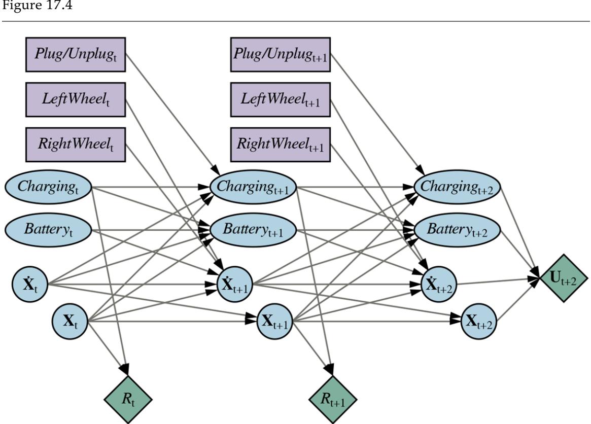
A dynamic decision network for a mobile robot with state variables for battery level, charging status, location, and velocity, and action variables for the left and right wheel motors and for charging.

The state space for the MDP is the Cartesian product of the ranges of these four variables. The action is now a set of action variables, comprised of , which has three values (plug, noop, and noop); LeftWheel for the power sent to the left wheel; and RightWheel for the power sent to the right wheel. The set of actions for the MDP is the Cartesian product of the ranges of these three variables. Notice that each action variable affects only a subset of the state variables.

The overall transition model is the conditional distribution , which can be computed as a product of conditional probabilities from the DDN. The reward here is a single variable that depends only on the location (for, say, arriving at a destination) and Charging, as the robot has to pay for electricity used; in this particular model, the reward doesn’t depend on the action or the outcome state.

The network in Figure 17.4 has been projected three steps into the future. Notice that the network includes nodes for the rewards for , , and , but the utility for . This is because the agent must maximize the (discounted) sum of all future rewards, and represents the reward for all rewards from onwards. If a heuristic approximation to is available, it can be included in the MDP representation in this way and used in lieu of further expansion. This approach is closely related to the use of bounded-depth search and heuristic evaluation functions for games in Chapter 5 .

Another interesting and well-studied MDP is the game of Tetris (Figure 17.5(a) ). The state variables for the game are the CurrentPiece, the NextPiece, and a bit-vector-valued variable Filled with one bit for each of the board locations. Thus, the state space has states. The DDN for Tetris is shown in Figure 17.5(b) . Note that is a deterministic function of and . It turns out that every policy for Tetris is proper (reaches a terminal state): eventually the board fills despite one’s best efforts to empty it.

Figure 17.5

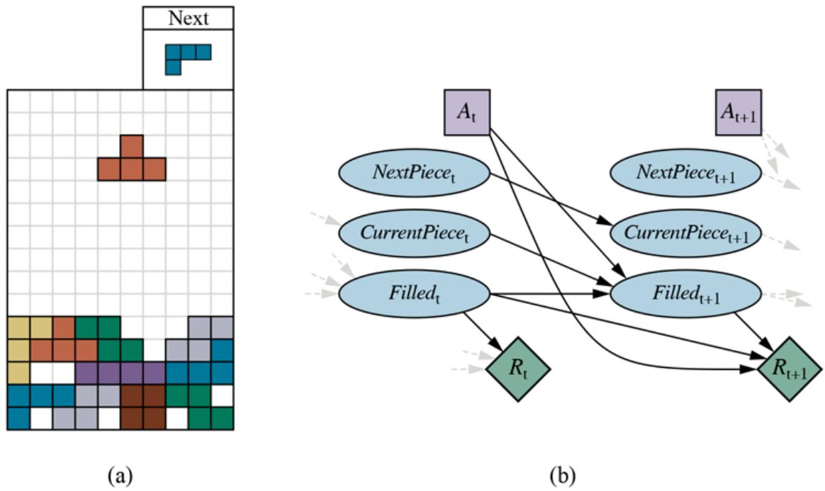
1. The game of Tetris. The T-shaped piece at the top center can be dropped in any orientation and in any horizontal position. If a row is completed, that row disappears and the rows above it move down, and the agent receives one point. The next piece (here, the L-shaped piece at top right) becomes the current piece, and a new next piece appears, chosen at random from the seven piece types. The game ends if the board fills up to the top. (b) The DDN for the Tetris MDP.

17.2 Algorithms for MDPs

In this section, we present four different algorithms for solving MDPs. The first three, value iteration, policy iteration, and linear programming, generate exact solutions offline. The fourth is a family of online approximate algorithms that includes Monte Carlo planning.

Monte Carlo planning

17.2.1 Value Iteration

Value iteration

The Bellman equation (Equation (17.5) ) is the basis of the value iteration algorithm for solving MDPs. If there are possible states, then there are Bellman equations, one for each state. The equations contain unknowns—the utilities of the states. So we would like to solve these simultaneous equations to find the utilities. There is one problem: the equations are nonlinear, because the ” ” operator is not a linear operator. Whereas systems of linear equations can be solved quickly using linear algebra techniques, systems of nonlinear equations are more problematic. One thing to try is an iterative approach. We start with arbitrary initial values for the utilities, calculate the right-hand side of the equation, and plug it into the left-hand side—thereby updating the utility of each state from the utilities of its neighbors. We repeat this until we reach an equilibrium.

Let be the utility value for state at the th iteration. The iteration step, called a Bellman update, looks like this:

(17.10)

\[U\_{i+1}(s) \leftarrow \max\_{a \in A(s)} \sum\_{s'} P(s'|s, a) [R(s, a, s') + \gamma U\_i(s')]\ ,\]

Bellman update

where the update is assumed to be applied simultaneously to all the states at each iteration. If we apply the Bellman update infinitely often, we are guaranteed to reach an equilibrium (see “convergence of value iteration” below), in which case the final utility values must be solutions to the Bellman equations. In fact, they are also the unique solutions, and the corresponding policy (obtained using Equation (17.4) ) is optimal. The detailed algorithm, including a termination condition when the utilities are “close enough,” is shown in Figure 17.6 . Notice that we make use of the Q-VALUE function defined on page 569.

Figure 17.6

The value iteration algorithm for calculating utilities of states. The termination condition is from Equation (17.12) .

We can apply value iteration to the world in Figure 17.1(a) . Starting with initial values of zero, the utilities evolve as shown in Figure 17.7(a) . Notice how the states at different distances from (4,3) accumulate negative reward until a path is found to (4,3), whereupon the utilities start to increase. We can think of the value iteration algorithm as propagating information through the state space by means of local updates.

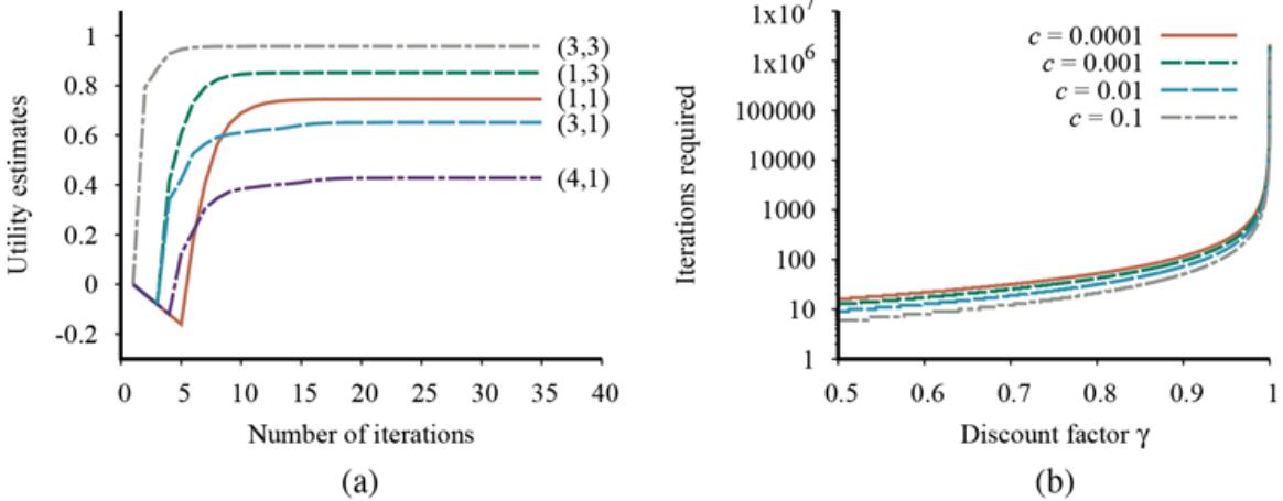
1. Graph showing the evolution of the utilities of selected states using value iteration. (b) The number of value iterations required to guarantee an error of at most for different values of , as a function of the discount factor .

Convergence of value iteration

We said that value iteration eventually converges to a unique set of solutions of the Bellman equations. In this section, we explain why this happens. We introduce some useful mathematical ideas along the way, and we obtain some methods for assessing the error in the utility function returned when the algorithm is terminated early; this is useful because it means that we don’t have to run forever. This section is quite technical.

The basic concept used in showing that value iteration converges is the notion of a contraction. Roughly speaking, a contraction is a function of one argument that, when applied to two different inputs in turn, produces two output values that are “closer together,” by at least some constant factor, than the original inputs. For example, the function “divide by two” is a contraction, because, after we divide any two numbers by two, their difference is halved. Notice that the “divide by two” function has a fixed point, namely zero, that is unchanged by the application of the function. From this example, we can discern two important properties of contractions:

• A contraction has only one fixed point; if there were two fixed points they would not get closer together when the function was applied, so it would not be a contraction.
• When the function is applied to any argument, the value must get closer to the fixed point (because the fixed point does not move), so repeated application of a contraction always reaches the fixed point in the limit.

Contraction

Now, suppose we view the Bellman update (Equation (17.10) ) as an operator that is applied simultaneously to update the utility of every state. Then the Bellman equation becomes and the Bellman update equation can be written as

Max norm

Next, we need a way to measure distances between utility vectors. We will use the max norm, which measures the “length” of a vector by the absolute value of its biggest component:

\[\|U\| = \max\_{\mathbf{u}} |U(s)|.\]

With this definition, the “distance” between two vectors, , is the maximum difference between any two corresponding elements. The main result of this section is the following: Let and be any two utility vectors. Then we have

(17.11)

\[\|B\boldsymbol{U}\_i - B\boldsymbol{U}\_i'\| \le \gamma \; \parallel \; \boldsymbol{U}\_i - \boldsymbol{U}\_i' \|.\]

That is, the Bellman update is a contraction by a factor of on the space of utility vectors. (Exercise 17.VICT provides some guidance on proving this claim.) Hence, from the properties of contractions in general, it follows that value iteration always converges to a unique solution of the Bellman equations whenever .

We can also use the contraction property to analyze the rate of convergence to a solution. In particular, we can replace in Equation (17.11) with the true utilities , for which . Then we obtain the inequality

\[||BU\_i - U\,|| \le \gamma \, ||\, U\_i - U\||.\]

If we view as the error in the estimate , we see that the error is reduced by a factor of at least on each iteration. Thus, value iteration converges exponentially fast. We can calculate the number of iterations required as follows: First, recall from Equation (17.1) that the utilities of all states are bounded by . This means that the maximum initial error . Suppose we run for iterations to reach an error of at most . Then, because the error is reduced by at least each time, we require . Taking logs, we find that

\[N = \lceil \log(2R\_{\text{max}}/\epsilon(1-\gamma))/\log(1/\gamma) \rceil\]

iterations suffice. Figure 17.7(b) shows how varies with , for different values of the ratio . The good news is that, because of the exponentially fast convergence, does not depend much on the ratio . The bad news is that grows rapidly as becomes close to 1. We can get fast convergence if we make small, but this effectively gives the agent a short horizon and could miss the long-term effects of the agent’s actions.

The error bound in the preceding paragraph gives some idea of the factors influencing the run time of the algorithm, but is sometimes overly conservative as a method of deciding when to stop the iteration. For the latter purpose, we can use a bound relating the error to the size of the Bellman update on any given iteration. From the contraction property (Equation (17.11) ), it can be shown that if the update is small (i.e., no state’s utility changes by much), then the error, compared with the true utility function, also is small. More precisely,

(17.12)

\[\text{if } \quad \|U\_{i+1} - U\_i\| < \epsilon (1 - \gamma)/\gamma \quad \text{then} \quad \|\|U\_{i+1} - U\|\| < \epsilon.\]

This is the termination condition used in the VALUE-ITERATION algorithm of Figure 17.6 .

Policy loss

So far, we have analyzed the error in the utility function returned by the value iteration algorithm. What the agent really cares about, however, is how well it will do if it makes its decisions on the basis of this utility function. Suppose that after iterations of value iteration, the agent has an estimate of the true utility and obtains the maximum expected utility (MEU) policy based on one-step look-ahead using (as in Equation (17.4) ). Will the resulting behavior be nearly as good as the optimal behavior? This is a crucial question for any real agent, and it turns out that the answer is yes. is the utility obtained if is executed starting in , and the policy loss is the most the agent can lose by executing instead of the optimal policy . The policy loss of is connected to the error in by the following inequality:

(17.13)

\[\text{if } \quad \|U\_i - U\| < \epsilon \quad \text{then} \quad \|\|U^{\pi\_i} - U\|\| < 2\epsilon.\]

In practice, it often occurs that becomes optimal long before has converged. Figure 17.8 shows how the maximum error in and the policy loss approach zero as the value iteration process proceeds for the environment with . The policy is optimal when , even though the maximum error in is still 0.51.

Figure 17.8

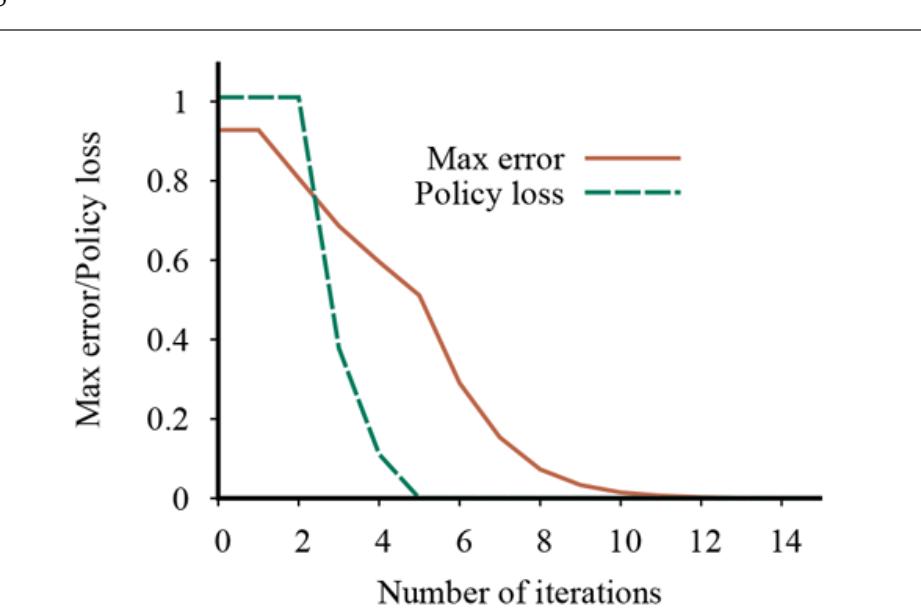
The maximum error of the utility estimates and the policy loss , as a function of the number of iterations of value iteration on the world.

Now we have everything we need to use value iteration in practice. We know that it converges to the correct utilities, we can bound the error in the utility estimates if we stop after a finite number of iterations, and we can bound the policy loss that results from executing the corresponding MEU policy. As a final note, all of the results in this section depend on discounting with . If and the environment contains terminal states, then a similar set of convergence results and error bounds can be derived.

17.2.2 Policy iteration

In the previous section, we observed that it is possible to get an optimal policy even when the utility function estimate is inaccurate. If one action is clearly better than all others, then the exact magnitude of the utilities on the states involved need not be precise. This insight suggests an alternative way to find optimal policies. The policy iteration algorithm alternates the following two steps, beginning from some initial policy :

• POLICY EVALUATION: given a policy , calculate , the utility of each state if were to be executed.
• POLICY IMPROVEMENT: Calculate a new MEU policy , using one-step look-ahead based on (as in Equation (17.4) ).

Policy iteration

Policy evaluation

Policy improvement

The algorithm terminates when the policy improvement step yields no change in the utilities. At this point, we know that the utility function is a fixed point of the Bellman update, so it is a solution to the Bellman equations, and must be an optimal policy.

Because there are only finitely many policies for a finite state space, and each iteration can be shown to yield a better policy, policy iteration must terminate. The algorithm is shown in Figure 17.9 . As with value iteration, we use the Q-VALUE function defined on page 569.

Figure 17.9

The policy iteration algorithm for calculating an optimal policy.

How do we implement POLICY-EVALUATION? It turns out that doing so is simpler than solving the standard Bellman equations (which is what value iteration does), because the action in each state is fixed by the policy. At the th iteration, the policy specifies the action in state . This means that we have a simplified version of the Bellman equation (17.5) relating the utility of (under ) to the utilities of its neighbors:

(17.14)

\[U\_i(s) = \sum\_{s'} P(s'|s, \pi\_i(s)) [R(s, \pi\_i(s), s') + \gamma U\_i(s')].\]

For example, suppose is the policy shown in Figure 17.2(a) . Then we have , , and so on, and the simplified Bellman equations are

\[\begin{aligned} U\_i(1,1) &= 0.8[-0.04 + U\_i(1,2)] + 0.1[-0.04 + U\_i(2,1) + 0.1[-0.04 + U\_i(1,1)]], \\ U\_i(1,2) &= 0.8[-0.04 + U\_i(1,3)] + 0.2[-0.04 + U\_i(1,2)], \end{aligned}\]

and so on for all the states. The important point is that these equations are linear, because the ” ” operator has been removed. For states, we have linear equations with unknowns, which can be solved exactly in time by standard linear algebra methods. If the transition model is sparse—that is, if each state transitions only to a small number of other states—then the solution process can be faster still.

For small state spaces, policy evaluation using exact solution methods is often the most efficient approach. For large state spaces, time might be prohibitive. Fortunately, it is not necessary to do exact policy evaluation. Instead, we can perform some number of simplified value iteration steps (simplified because the policy is fixed) to give a reasonably good approximation of the utilities. The simplified Bellman update for this process is

\[U\_{i+1}(s) \leftarrow \sum\_{s'} P(s'|s, \pi\_i(s)) [R(s, \pi\_i(s), s') + \gamma \, U\_i(s')],\]

and this is repeated several times to efficiently produce the next utility estimate. The resulting algorithm is called modified policy iteration.

Modified policy iteration

The algorithms we have described so far require updating the utility or policy for all states at once. It turns out that this is not strictly necessary. In fact, on each iteration, we can pick any subset of states and apply either kind of updating (policy improvement or simplified value iteration) to that subset. This very general algorithm is called asynchronous policy iteration. Given certain conditions on the initial policy and initial utility function, asynchronous policy iteration is guaranteed to converge to an optimal policy. The freedom to choose any states to work on means that we can design much more efficient heuristic algorithms—for example, algorithms that concentrate on updating the values of states that are likely to be reached by a good policy. There’s no sense planning for the results of an action you will never do.

Asynchronous policy iteration

17.2.3 Linear programming

Linear programming or LP, which was mentioned briefly in Chapter 4 (page 121), is a general approach for formulating constrained optimization problems, and there are many industrial-strength LP solvers available. Given that the Bellman equations involve a lot of sums and maxes, it is perhaps not surprising that solving an MDP can be reduced to solving a suitably formulated linear program.

The basic idea of the formulation is to consider as variables in the LP the utilities of each state , noting that the utilities for an optimal policy are the highest utilities attainable that are consistent with the Bellman equations. In LP language, that means we seek to minimize for all subject to the inequalities

\[U(s) \ge \sum\_{s'} P(s'|s, a) [R(s, a, s') + \gamma U(s')]\]

for every state and every action .

This creates a connection from dynamic programming to linear programming, for which algorithms and complexity issues have been studied in great depth. For example, from the fact that linear programming is solvable in polynomial time, one can show that MDPs can be solved in time polynomial in the number of states and actions and the number of bits required to specify the model. In practice, it turns out that LP solvers are seldom as efficient as dynamic programming for solving MDPs. Moreover, polynomial time may sound good, but the number of states is often very large. Finally, it’s worth remembering that even the simplest and most uninformed of the search algorithms in Chapter 3 runs in linear time in the number of states and actions.

17.2.4 Online algorithms for MDPs

Value iteration and policy iteration are offline algorithms: like the A* algorithm in Chapter 3 , they generate an optimal solution for the problem, which can then be executed by a simple agent. For sufficiently large MDPs, such as the Tetris MDP with states, exact

offline solution, even by a polynomial-time algorithm, is not possible. Several techniques have been developed for approximate offline solution of MDPs; these are covered in the notes at the end of the chapter and in Chapter 22 (Reinforcement Learning).

Here we will consider online algorithms, analogous to those used for game playing in Chapter 5 , where the agent does a significant amount of computation at each decision point rather than operating primarily with precomputed information.

The most straightforward approach is actually a simplification of the EXPECTIMINIMAX algorithm for game trees with chance nodes: the EXPECTIMAX algorithm builds a tree of alternating max and chance nodes, as illustrated in Figure 17.10 . (There is a slight difference from standard EXPECTIMINIMAX in that there are rewards on nonterminal as well as terminal transitions.) An evaluation function can be applied to the nonterminal leaves of the tree, or they can be given a default value. A decision can be extracted from the search tree by backing up the utility values from the leaves, taking an average at the chance nodes and taking the maximum at the decision nodes.

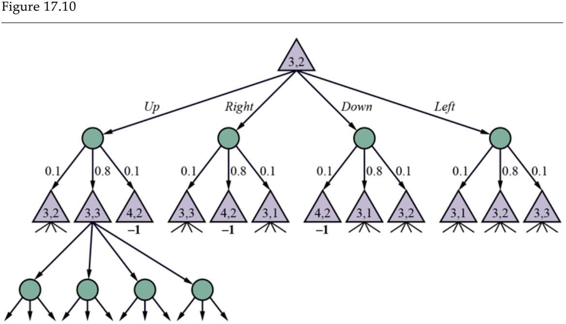
Part of an expectimax tree for the MDP rooted at (3,2). The triangular nodes are max modes and the circular nodes are chance nodes.

For problems in which the discount factor is not too close to 1, the -horizon is a useful concept. Let be a desired bound on the absolute error in the utilities computed from an

expectimax tree of bounded depth, compared to the exact utilities in the MDP. Then the horizon is the tree depth such that the sum of rewards beyond any leaf at that depth is less than —roughly speaking, anything that happens after is irrelevant because it’s so far in the future. Because the sum of rewards beyond is bounded by , a depth of suffices. So, building a tree to this depth gives near-optimal decisions. For example, with , , and , we find , which seems reasonable. On the other hand, if , , which seems less reasonable!

In addition to limiting the depth, it is also possible to avoid the potentially enormous branching factor at the chance nodes. (For example, if all the conditional probabilities in a DBN transition model are nonzero, the transition probabilities, which are given by the product of the conditional probabilities, are also nonzero, meaning that every state has some probability of transitioning to every other state.)

As noted in Section 13.4 , expectations with respect to a probability distribution can be approximated by generating samples from and using the sample mean. In mathematical form, we have

\[\sum\_{x} P(x)f(x) \approx \frac{1}{N} \sum\_{i=1}^{N} f(x\_i).\]

So, if the branching factor is very large, meaning that there are very many possible values, a good approximation to the value of the chance node can be obtained by sampling a bounded number of outcomes from the action. Typically, the samples will focus on the most likely outcomes because those are most likely to be generated.

If you look closely at the tree in Figure 17.10 , you will notice something: it isn’t really a tree. For example, the root (3,2) is also a leaf, so one ought to consider this as a graph, and one ought to constrain the value of the leaf (3,2) to be the same as the value of the root (3,2), since they are the same state. In fact, this line of thinking quickly brings us back to the Bellman equations that relate the values of states to the values of neighboring states. The explored states actually constitute a sub-MDP of the original MDP, and this sub-MDP can be solved using any of the algorithms in this chapter to yield a decision for the current state. (Frontier states are typically given a fixed estimated value.)

This general approach is called real-time dynamic programming (RTDP) and is quite analogous to LRTA* in Chapter 4 . Algorithms of this kind can be quite effective in moderate-sized domains such as grid worlds; in larger domains such as Tetris, there are two issues. First, the state space is such that any manageable set of explored states contains very few repeated states, so one might as well use a simple expectimax tree. Second, a simple heuristic for frontier nodes may not be enough to guide the agent, particularly if rewards are sparse.

Real-time dynamic programming (RTDP)

One possible fix is to apply reinforcement learning to generate a much more accurate heuristic (see Chapter 22 ). Another approach is to look further ahead in the MDP using the Monte Carlo approach of Section 5.4 . In fact, the UCT algorithm from Figure 5.10 was developed originally for MDPs rather than games. The changes required to solve MDPs rather than games are minimal: they arise primarily from the fact that the opponent (nature) is stochastic and from the need to keep track of rewards rather than just wins and losses.

When applied to the world, the performance of UCT is not especially impressive. As Figure 17.11 shows, it takes 160 playouts on average to reach a total reward of 0.4, whereas an optimal policy has an expected total reward of 0.7453 from the initial state (see Figure 17.3 ). One reason UCT can have difficulty is that is builds a tree rather than a graph and uses (an approximation to) expectimax rather than dynamic programming. The world is very “loopy”: although there are only 9 nonterminal states, UCT’s playouts often continue for more than 50 actions.

Figure 17.11

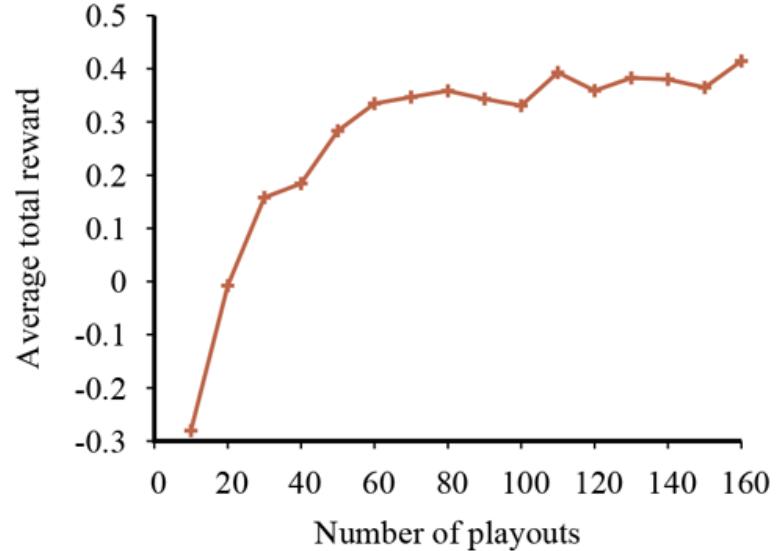
Performance of UCT as a function of the number of playouts per move for the world using a random playout policy, averaged over 1000 runs per data point.

UCT seems better suited for Tetris, where the playouts go far enough into the future to give the agent a sense of whether a potentially risky move will work out in the end or cause a massive pile-up. Exercise 17.UCTT explores the application of UCT to Tetris. One particularly interesting question is how much a simple simulation policy can help—for example, one that avoids creating overhangs and puts pieces as low as possible.

17.3 Bandit Problems

In Las Vegas, a one-armed bandit is a slot machine. A gambler can insert a coin, pull the lever, and collect the winnings (if any). An -armed bandit has levers. Behind each lever is a fixed but unknown probability distribution of winnings; each pull samples from that unknown distribution.

N-armed bandit

The gambler must choose which lever to play on each successive coin—the one that has paid off best, or maybe one that has not been tried yet? This is an example of the ubiquitous tradeoff between exploitation of the current best action to obtain rewards and exploration of previously unknown states and actions to gain information, which can in some cases be converted into a better policy and better long-term rewards. In the real world, one constantly has to decide between continuing in a comfortable existence, versus striking out into the unknown in the hopes of a better life.

The -armed bandit problem is a formal model for real problems in many vitally important areas, such as deciding which of possible new treatments to try to cure a disease, which of possible investments to put part of your savings into, which of possible research projects to fund, or which of possible advertisements to show when the user visits a particular web page.

Early work on the problem began in the U.S. during World War II; it proved so recalcitrant that Allied scientists proposed that “the problem be dropped over Germany, as the ultimate instrument of intellectual sabotage” (Whittle, 1979).

It turns out that the scientists, both during and after the war, were trying to prove “obviously true” facts about bandit problems that are, in fact, false. (As Bradt et al. (1956) put it, “There are many nice properties which optimal strategies do not possess.”) For example, it was

generally assumed that an optimal policy would eventually settle on the best arm in the long run; in fact, there is a finite probability that an optimal policy settles on a suboptimal arm. We now have a solid theoretical understanding of bandit problems as well as useful algorithms for solving them.

There are several different definitions of bandit problems; one of the cleanest and most general is as follows:

• Each arm is a Markov reward process or MRP, that is, an MDP with only one possible action . It has states , transition model , and reward . The arm defines a distribution over sequences of rewards , where each is a random variable.
• The overall bandit problem is an MDP: the state space is given by the Cartesian product ; the actions are ; the transition model updates the state of whichever arm is selected, according to its specific transition model, leaving the other arms unchanged; and the discount factor is .

Bandit problems

Markov reward process

This definition is very general, covering a wide range of cases. The key property is that the arms are independent, coupled only by the fact that the agent can work on only one arm at a time. It’s possible to define a still more general version in which fractional efforts can be applied to all arms simultaneously, but the total effort across all arms is bounded; the basic results described here carry over to this case.

We will see shortly how to formulate a typical bandit problem within this framework, but let’s warm up with the simple special case of deterministic reward sequences. Let , and suppose that there are two arms labeled and . Pulling multiple times yields the sequence of rewards , while pulling yields (Figure 17.12(a) ). If, at the beginning, one had to commit to one arm or the other and stick with it, the choice would be made by computing the utility (total discounted reward) for each arm:

\[\begin{aligned} U(M) &= \{1.0 \times 0\} + \{0.5 \times 2\} + \{0.5^2 \times 0\} + \{0.5^3 \times 7.2\} = 1.9\\ U(M\_1) &= \sum\_{t=0}^{\infty} 0.5^t = 2.0. \end{aligned}\]

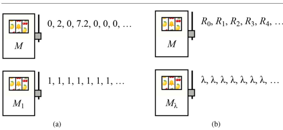
1. A simple deterministic bandit problem with two arms. The arms can be pulled in any order, and each yields the sequence of rewards shown. (b) A more general case of the bandit in (a), where the first arm gives an arbitrary sequence of rewards and the second arm gives a fixed reward .

One might think the best choice is to go with , but a moment’s more thought shows that starting with and then switching to after the fourth reward gives the sequence , for which

\[U(S) = \left(1.0 \times 0\right) + \left(0.5 \times 2\right) + \left(0.5^2 \times 0\right) + \left(0.5^3 \times 7.2\right) + \sum\_{t=4}^{\infty} 0.5^t = 2.025.5\]

Hence the strategy that switches from to at the right time is better than either arm individually. In fact, is optimal for this problem: all other switching times give less reward.

One-armed bandit

Figure 17.12

Let’s generalize this case slightly, so that now the first arm yields an arbitrary sequence (which may be known or unknown) and the second arm yields for some known fixed constant (see Figure 17.12(b) ). This is called a one-armed bandit in the literature, because it is formally equivalent to the case where there is one arm that produces rewards and costs for each pull. (Pulling arm is equivalent to not pulling , so it gives up a reward of each time.) With just one arm, the only choice is to whether to pull again or to stop. If you pull the first arm times (i.e., at times we say that the stopping time is .

Stopping time

Going back to our version with and , let’s assume that after pulls of the first arm, an optimal strategy eventually pulls the second arm for the first time. Since no information is gained from this move (we already know the payoff will be ), at time we will be in the same situation and thus an optimal strategy must make the same choice.

Equivalently, we can say that an optimal strategy is to run arm up to time and then switches to for the rest of time. It’s possible that if the strategy chooses immediately, or if the strategy never chooses , or somewhere in between. Now let’s consider the value of such that an optimal strategy is exactly indifferent between (a) running up to the best possible stopping time and then switching to forever, and (b) choosing immediately. At the tipping point we have

\[\max\_{T>0} \mathcal{E}\left[\left(\sum\_{t=0}^{T-1} \gamma^t R\_t\right) + \sum\_{t=T}^{\infty} \gamma^t \lambda\right] = \sum\_{t=0}^{\infty} \gamma^t \lambda, \quad \lambda \in \mathbb{R}\]

which simplifies to

(17.15)

\[\lambda = \max\_{T>0} \frac{E\left(\sum\_{t=0}^{T-1} \gamma^t R\_t\right)}{E\left(\sum\_{t=0}^{T-1} \gamma^t\right)}.\]

This equation defines a kind of “value” for in terms of its ability to deliver a stream of timely rewards; the numerator of the fraction represents a utility while the denominator can be thought of as a “discounted time,” so the value describes the maximum obtainable utility per unit of discounted time. (It’s important to remember that in the equation is a stopping time, which is governed by a rule for stopping rather than being a simple integer; it reduces to a simple integer only when is a deterministic reward sequence.) The value defined in Equation (17.15) is called the Gittins index of .

Gittins index

The remarkable thing about the Gittins index is that it provides a very simple optimal policy for any bandit problem: pull the arm that has the highest Gittins index, then update the Gittins indices. Furthermore, because the index of arm depends only on the properties of that arm, an optimal decision on the first iteration can be calculated in time, where is the number of arms. And because the Gittins indices of the arms that are not selected remain unchanged, each decision after the first one can be calculated in time.

17.3.1 Calculating the Gittins index

To get more of a feel for the index, let’s calculate the value of the numerator, denominator, and ratio in Equation (17.15) for different possible stopping times on the deterministic reward sequence :

		2	3	ব	5	0
R,	0		0	7.2	0	0
ΣΥ Rt 0.0 1.0			1.0	1.9	1.9	1.9
ΣΥ		1.0 1.5	1.75	1.875		1.9375 1.9687
ratio						0.0 0.6667 0.5714 1.0133 0.9806 0.9651

Clearly, the ratio will decrease from here on, because the numerator remains constant while the denominator continues to increase. Thus, the Gittins index for this arm is 1.0133, the maximum value attained by the ratio. In combination with a fixed arm with

, the optimal policy collects the first four rewards from and then switches to . For , the optimal policy always chooses .

To calculate the Gittins index for a general arm with current state , we simply make the following observation: at the tipping point where an optimal policy is indifferent between choosing arm and choosing the fixed arm , the value of choosing is the same as the value of choosing an infinite sequence of -rewards.

Suppose we augment so that at each state in , the agent has two choices: either continue with as before, or quit and receive an infinite sequence of -rewards (see Figure 17.13(a) ). This turns into an MDP, whose optimal policy is just the optimal stopping rule for . Hence the value of an optimal policy in this new MDP is equal to the value of an infinite sequence of -rewards, that is, . So we can just solve this MDP … but, unfortunately, we don’t know the value of to put into the MDP, as this is precisely what we are trying to calculate. But we do know that, at the tipping point, an optimal policy is indifferent between and , so we could replace the choice to get an infinite sequence of -rewards with the choice to go back and restart from its initial state . (More precisely, we add a new action in every state that has the same rewards and outcomes as the action available in ; see Exercise 17.KATV.) This new MDP , called a restart MDP, is illustrated in Figure 17.13(b) .

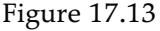
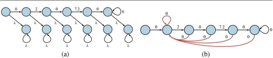
1. The reward sequence augmented with a choice to switch permanently to a constant arm at each point. (b) An MDP whose optimal value is exactly equivalent to the optimal value for (a), at the point where the optimal policy is indifferent between and .

Restart MDP

We have the general result that the Gittins index for an arm in state is equal to times the value of an optimal policy for the restart MDP . This MDP can be solved by any of the algorithms in Section 17.2 . Value iteration applied to in Figure 17.13(b) gives a value of 2.0266 for the start state, so we have as before.

17.3.2 The Bernoulli bandit

Perhaps the simplest and best-known instance of a bandit problem is the Bernoulli bandit, where each arm produces a reward of 0 or 1 with a fixed but unknown probability . The state of arm is defined by and , the counts of successes (1s) and failures (0s) so far for that arm; the transition probability predicts the next outcome to be 1 with probability and 0 with probability . The counts are initialized to 1 so that the initial probabilities are 1/2 rather than 0/0. The Markov reward process is shown in Figure 17.14(a) . 4

4 The probabilities are those of a Bayesian updating process with a Beta(1,1) prior (see Section 20.2.5 ).

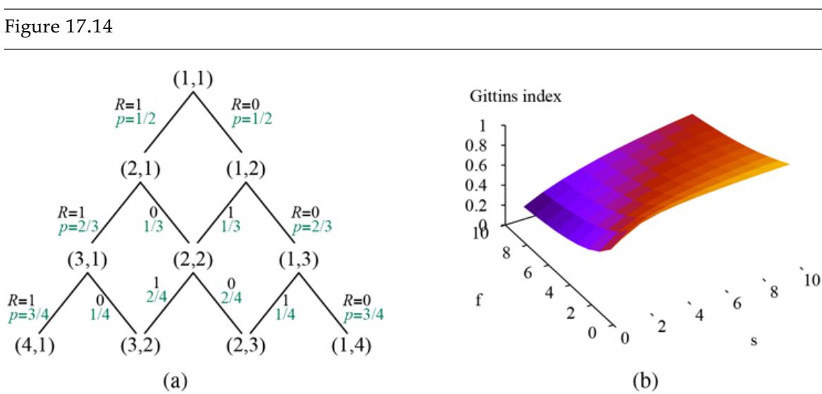
1. States, rewards, and transition probabilities for the Bernoulli bandit. (b) Gittins indices for the states of the Bernoulli bandit process.

Bernoulli bandit

We cannot quite apply the transformation of the preceding section to calculate the Gittins index of the Bernoulli arm because it has infinitely many states. We can, however, obtain a very accurate approximation by solving the truncated MDP with states up to and . The results are shown in Figure 17.14(b) . The results are intuitively reasonable: we see that, generally speaking, arms with higher payoff probabilities are preferred, but there is also an exploration bonus associated with arms that have only been tried a few times. For example, the index for the state (3,2) is higher than the index for the state (7,4) (0.7057 vs. 0.6922), even though the estimated value at (3,2) is lower (0.6 vs. 0.6364).

Exploration bonus

17.3.3 Approximately optimal bandit policies

Calculating Gittins indices for more realistic problems is rarely easy. Fortunately, the general properties observed in the preceding section—namely, the desirability of some combination of estimated value and uncertainty—lend themselves to the creation of simple policies that turn out to be “nearly as good” as optimal policies.

The first class of methods uses the upper confidence bound or UCB heuristic, previously introduced for Monte Carlo tree search (Figure 5.11 on page 163). The basic idea is to use the samples from each arm to establish a confidence interval for the value of the arm, that is, a range within which the value can be estimated to lie with high confidence; then choose the arm with the highest upper bound on its confidence interval. The upper bound is the current mean value estimate plus some multiple of the standard deviation of the uncertainty in the value. The standard deviation is proportional to , where is the number of times arm has been sampled. So we have an approximate index value for arm given by

\[UCB(M\_i) = \hat{\mu}\_i + g(N) / \sqrt{N\_i} \ ,\]

Upper confidence bound

where is an appropriately chosen function of , the total number of samples drawn from all arms. A UCB policy simply picks the arm with the highest UCB value. Notice that the UCB value is not strictly an index because it depends on , the total number of samples drawn across all arms, and not just on the arm itself.

The precise definition of determines the regret relative to the clairvoyant policy, which simply picks the best arm and yields average reward . A famous result due to Lai and Robbins (1985) shows that, for the undiscounted case, no possible algorithm can have regret that grows more slowly than . Several different choices of lead to a UCB policy that matches this growth; for example, we can use .

A second method, Thompson sampling (Thompson, 1933), chooses chooses an arm randomly according to the probability that the arm is in fact optimal, given the samples so far. Suppose that is the current probability distribution for the true value of arm . Then a simple way to implement Thompson sampling is to generate one sample from each and then pick the best sample. This algorithm also has a regret that grows as .

Thompson sampling

17.3.4 Non-indexable variants

Bandit problems were motivated in part by the task of testing new medical treatments on seriously ill patients. For this task, the goal of maximizing the total number of successes over time clearly makes sense: each successful test means a life saved, each failure a life lost.

If we change the assumptions slightly, however, a different problem emerges. Suppose that, instead of determining the best medical treatment for each new human patient, we are instead testing different drugs on samples of bacteria with the goal of deciding which drug is best. We will then put that drug into production and forgo the others. In this scenario there

is no additional cost if the bacteria dies—there is a fixed cost for each test, but we don’t have to minimize test failures; rather we are just trying to make a good decision as fast as possible.

The task of choosing the best option under these conditions is called a selection problem. Selection problems are ubiquitous in industrial and personnel contexts. One often must decide which supplier to use for a process; or which candidate employees to hire. Selection problems are superficially similar to the bandit problem but have different mathematical properties. In particular, no index function exists for selection problems. The proof of this fact requires showing any scenario where the optimal policy switches its preferences for two arms and when a third arm is added (see Exercise 17.SELC).

Selection problem

Chapter 5 introduced the concept of metalevel decision problems such as deciding what computations to make during a game-tree search prior to making a move. A metalevel decision of this kind is also a selection problem rather than a bandit problem. Clearly, a node expansion or evaluation costs the same amount of time whether it produces a high or a low output value. It is perhaps surprising, then, that the Monte Carlo tree search algorithm (see page 163) has been so successful, given that it tries to solve selection problems with the UCB heuristic, which was designed for bandit problems. Generally speaking, one expects optimal bandit algorithms to explore much less than optimal selection algorithms, because the bandit algorithm assumes that a failed trial costs real money.

An important generalization of the bandit process is the bandit superprocess or BSP, in which each arm is a full Markov decision process in its own right, rather than being a Markov reward process with only one possible action. All other properties remain the same: the arms are independent, only one (or a bounded number) can be worked on at a time, and there is a single discount factor.

Bandit superprocess

Examples of BSPs include daily life, where one can attend to one task at a time, even though several tasks may need attention; project management with multiple projects; teaching with multiple pupils needing individual guidance; and so on. The ordinary term for this is multitasking. It is so ubiquitous as to be barely noticeable: when formulating a real-world decision problem, decision analysts rarely ask if their client has other, unrelated problems.

Multitasking

One might reason as follows: “If there are disjoint MDPs then it is obvious that an optimal policy overall is built from the optimal solutions of the individual MDPs. Given its optimal policy , each MDP becomes a Markov reward process where there is only one action in each state . So we have reduced the -armed bandit superprocess to an -armed bandit process.” For example, if a real-estate developer has one construction crew and several shopping centers to build, it seems to be just common sense that one should devise the optimal construction plan for each shopping center and then solve the bandit problem to decide where to send the crew each day.

While this sounds highly plausible, it is incorrect. In fact, the globally optimal policy for a BSP may include actions that are locally suboptimal from the point of view of the constituent MDP in which they are taken. The reason for this is that the availability of other MDPs in which to act changes the balance between short-term and long-term rewards in a component MDP. In fact, it tends to lead to greedier behavior in each MDP (seeking shortterm rewards) because aiming for long-term reward in one MDP would delay rewards in all the other MDPs.

BSP

For example, suppose the locally optimal construction schedule for one shopping center has the first shop available for rent by week 15, whereas a suboptimal schedule costs more but has the first shop available by week 5. If there are four shopping centers to build, it might be better to use the locally suboptimal schedule in each so that rents start coming in from weeks 5, 10, 15, and 20, rather than weeks 15, 30, 45, and 60. In other words, what would be only a 10-week delay for a single MDP turns into a 40-week delay for the fourth MDP. In general, the globally and locally optimal policies necessarily coincide only when the discount factor is 1; in that case, there is no cost to delaying rewards in any MDP.

The next question is how to solve BSPs. Obviously, the globally optimal solution for a BSP could be computed by converting it into a global MDP on the Cartesian-product state space. The number of states would be exponential in the number of arms of the BSP, so this would be horrendously impractical.

Instead, we can take advantage of the loose nature of the interaction between the arms. This interaction arises only from the agent’s limited ability to attend to the arms simultaneously. To some extent, the interaction can be modeled by the notion of opportunity cost: how much utility is given up per time step by not devoting that time step to another arm. The higher the opportunity cost, the more necessary it is to generate early rewards in a given arm. In some cases, an optimal policy in a given arm is unaffected by the opportunity cost. (Trivially, this is true in a Markov reward process because there is only one policy.) In that case, an optimal policy can be applied, converting that arm into a Markov reward process.

Opportunity cost

Such an optimal policy, if it exists, is called a dominating policy. It turns out that by adding actions to states, it is always possible to create a relaxed version of an MDP (see Section 3.6.2 ) so that it has a dominating policy, which thus gives an upper bound on the value of acting in the arm. A lower bound can be computed by solving each arm separately (which may yield a suboptimal policy overall) and then computing the Gittins indices. If the lower bound for acting in one arm is higher than the upper bounds for all other actions, then the problem is solved; if not, then a combination of look-ahead search and recomputation of

bounds is guaranteed to eventually identify an optimal policy for the BSP. With this approach, relatively large BSPs ( states or more) can be solved in a few seconds.

Dominating policy

17.4 Partially Observable MDPs

The description of Markov decision processes in Section 17.1 assumed that the environment was fully observable. With this assumption, the agent always knows which state it is in. This, combined with the Markov assumption for the transition model, means that the optimal policy depends only on the current state.

When the environment is only partially observable, the situation is, one might say, much less clear. The agent does not necessarily know which state it is in, so it cannot execute the action recommended for that state. Furthermore, the utility of a state and the optimal action in depend not just on , but also on how much the agent knows when it is in . For these reasons, partially observable MDPs (or POMDPs—pronounced “pom-dee-pees”) are usually viewed as much more difficult than ordinary MDPs. We cannot avoid POMDPs, however, because the real world is one.

Partially observable MDP

17.4.1 Definition of POMDPs

To get a handle on POMDPs, we must first define them properly. A POMDP has the same elements as an MDP—the transition model , actions , and reward function —but, like the partially observable search problems of Section 4.4 , it also has a sensor model . Here, as in Chapter 14 , the sensor model specifies the probability of perceiving evidence in state . For example, we can convert the world of Figure 17.1 into a POMDP by adding a noisy or partial sensor instead of assuming that the agent knows its location exactly. The noisy four-bit sensor from page 476 could be used, which reports the presence or absence of a wall in each compass direction with accuracy . 5

5 The sensor model can also depend on the action and outcome state, but this change is not fundamental.

As with MDPs, we can obtain compact representations for large POMDPs by using dynamic decision networks (see Section 17.1.4 ). We add sensor variables , assuming that the

state variables may not be directly observable. The POMDP sensor model is then given by . For example, we might add sensor variables to the DDN in Figure 17.4 such as BatteryMeter to estimate the actual charge Battery and Speedometer to estimate the magnitude of the velocity vector . A sonar sensor Walls might give estimated distances to the nearest wall in each of the four cardinal directions relative to the robot’s current orientation; these values depends on the current position and orientation . t t t t

In Chapters 4 and 11 , we studied nondeterministic and partially observable planning problems and identified the belief state—the set of actual states the agent might be in—as a key concept for describing and calculating solutions. In POMDPs, the belief state becomes a probability distribution over all possible states, just as in Chapter 14 . For example, the initial belief state for the POMDP could be the uniform distribution over the nine nonterminal states along with 0s for the terminal states, that is,

We use the notation to refer to the probability assigned to the actual state by belief state . The agent can calculate its current belief state as the conditional probability distribution over the actual states given the sequence of percepts and actions so far. This is essentially the filtering task described in Chapter 14 . The basic recursive filtering equation (14.5 on page 467) shows how to calculate the new belief state from the previous belief state and the new evidence. For POMDPs, we also have an action to consider, but the result is essentially the same. If was the previous belief state, and the agent does action and then perceives evidence , then the new belief state is obtained by calculating the probability of now being in state , for each , with the following formula:

\[b'(s') = \alpha \, P(e|s') \sum\_{s} P(s'|s, a) b(s) \,, \, \]

where is a normalizing constant that makes the belief state sum to 1. By analogy with the update operator for filtering (page 467), we can write this as

(17.16)

\[b' = \alpha \,\text{Fonwann}(b, a, e).\]

In the POMDP, suppose the agent moves Left and its sensor reports one adjacent wall; then it’s quite likely (although not guaranteed, because both the motion and the sensor are

noisy) that the agent is now in (3,1). Exercise 17.POMD asks you to calculate the exact probability values for the new belief state.

The fundamental insight required to understand POMDPs is this: the optimal action depends only on the agent’s current belief state. That is, an optimal policy can be described by a mapping from belief states to actions. It does not depend on the actual state the agent is in. This is a good thing, because the agent does not know its actual state; all it knows is the belief state. Hence, the decision cycle of a POMDP agent can be broken down into the following three steps:

• 1. Given the current belief state , execute the action .
• 2. Observe the percept .
• 3. Set the current belief state to and repeat.

We can think of POMDPs as requiring a search in belief-state space, just like the methods for sensorless and contingency problems in Chapter 4 . The main difference is that the POMDP belief-state space is continuous, because a POMDP belief state is a probability distribution. For example, a belief state for the world is a point in an 11-dimensional continuous space. An action changes the belief state, not just the physical state, because it affects the percept that is received. Hence, the action is evaluated at least in part according to the information the agent acquires as a result. POMDPs therefore include the value of information (Section 16.6 ) as one component of the decision problem.

Let’s look more carefully at the outcome of actions. In particular, let’s calculate the probability that an agent in belief state reaches belief state after executing action . Now, if we knew the action and the subsequent percept, then Equation (17.16) would provide a deterministic update to the belief state: . Of course, the subsequent percept is not yet known, so the agent might arrive in one of several possible belief states , depending on the percept that is received. The probability of perceiving , given that was performed starting in belief state , is given by summing over all the actual states that the agent might reach:

\[\begin{aligned} P(e|a,b) &= \sum\_{s'} P(e|a,s',b)P(s'|a,b) \\ &= \sum\_{s'} P(e|s')P(s'|a,b) \\ &= \sum\_{s'} P(e|s') \sum\_{s} P(s'|s,a)b(s) \end{aligned}\]

Let us write the probability of reaching from , given action , as . This probability can be calculated as follows:

(17.17)

\[\begin{aligned} P(b'|b,a) &= \sum\_{e} P(b'|e,a,b)P(e|a,b) \\ &= \sum\_{e} P(b'|e,a,b) \sum\_{s'} P(e|s') \sum\_{s} P(s'|s,a)b(s), \end{aligned}\]

where is 1 if and 0 otherwise.

Equation (17.17) can be viewed as defining a transition model for the belief-state space. We can also define a reward function for belief-state transitions, which is derived from the expected reward of the real state transitions that might be occurring. Here, we use the simple form , the expected reward if the agent does in belief state :

\[\rho(b,a) = \sum\_{s} b(s) \sum\_{s'} P(s'|s,a) R(s,a,s').\]

Together, and define an observable MDP on the space of belief states. Furthermore, it can be shown that an optimal policy for this MDP, , is also an optimal policy for the original POMDP. In other words, solving a POMDP on a physical state space can be reduced to solving an MDP on the corresponding belief-state space. This fact is perhaps less surprising if we remember that the belief state is always observable to the agent, by definition.

17.5 Algorithms for Solving POMDPs

We have shown how to reduce POMDPs to MDPs, but the MDPs we obtain have a continuous (and usually high-dimensional) state space. This means we will have to redesign the dynamic programming algorithms from Sections 17.2.1 and 17.2.2 , which assumed a finite state space and a finite number of actions. Here we describe a value iteration algorithm designed specifically for POMDPs, followed by an online decision-making algorithm similar to those developed for games in Chapter 5 .

17.5.1 Value iteration for POMDPs

Section 17.2.1 described a value iteration algorithm that computed one utility value for each state. With infinitely many belief states, we need to be more creative. Consider an optimal policy and its application in a specific belief state : the policy generates an action, then, for each subsequent percept, the belief state is updated and a new action is generated, and so on. For this specific , therefore, the policy is exactly equivalent to a conditional plan, as defined in Chapter 4 for nondeterministic and partially observable problems. Instead of thinking about policies, let us think about conditional plans and how the expected utility of executing a fixed conditional plan varies with the initial belief state. We make two observations:

• 1. Let the utility of executing a fixed conditional plan starting in physical state be . Then the expected utility of executing in belief state is just , or if we think of them both as vectors. Hence, the expected utility of a fixed conditional plan varies linearly with ; that is, it corresponds to a hyperplane in belief space.
• 2. At any given belief state , an optimal policy will choose to execute the conditional plan with highest expected utility; and the expected utility of under an optimal policy is just the utility of that conditional plan: . If an optimal policy chooses to execute starting at , then it is reasonable to expect that it might choose to execute in belief states that are very close to ; in fact, if we bound the depth of the conditional plans, then there are only finitely many such plans and the continuous space of belief states will generally be divided into regions, each corresponding to a particular conditional plan that is optimal in that region.

From these two observations, we see that the utility function on belief states, being the maximum of a collection of hyperplanes, will be piecewise linear and convex.

To illustrate this, we use a simple two-state world. The states are labeled and and there are two actions: Stay stays put with probability 0.9 and Go switches to the other state with probability 0.9. The rewards are and ; that is, any transition ending in has reward zero and any transition ending in has reward 1. For now we will assume the discount factor . The sensor reports the correct state with probability 0.6. Obviously, the agent should Stay when it’s in state and Go when it’s in state . The problem is that it doesn’t know where it is!

The advantage of a two-state world is that the belief space can be visualized in one dimension, because the two probabilities and sum to 1. In Figure 17.15(a) , the axis represents the belief state, defined by , the probability of being in state . Now let us consider the one-step plans and , each of which receives the reward for one transition as follows:

\[\begin{aligned} \alpha\_{[Stay]}(A) &= 0.9R(A, Stay, A) + 0.1R(A, Stay, B) = 0.1\\ \alpha\_{[Stay]}(B) &= 0.1R(B, Stay, A) + 0.9R(B, Stay, B) = 0.9 \\ \alpha\_{[Go]}(A) &= 0.1R(A, Go, A) + 0.9R(A, Go, B) = 0.9 \\ \alpha\_{[Go]}(B) &= 0.9R(B, Go, A) + 0.1R(B, Go, B) = 0.1 \end{aligned}\]

Figure 17.15

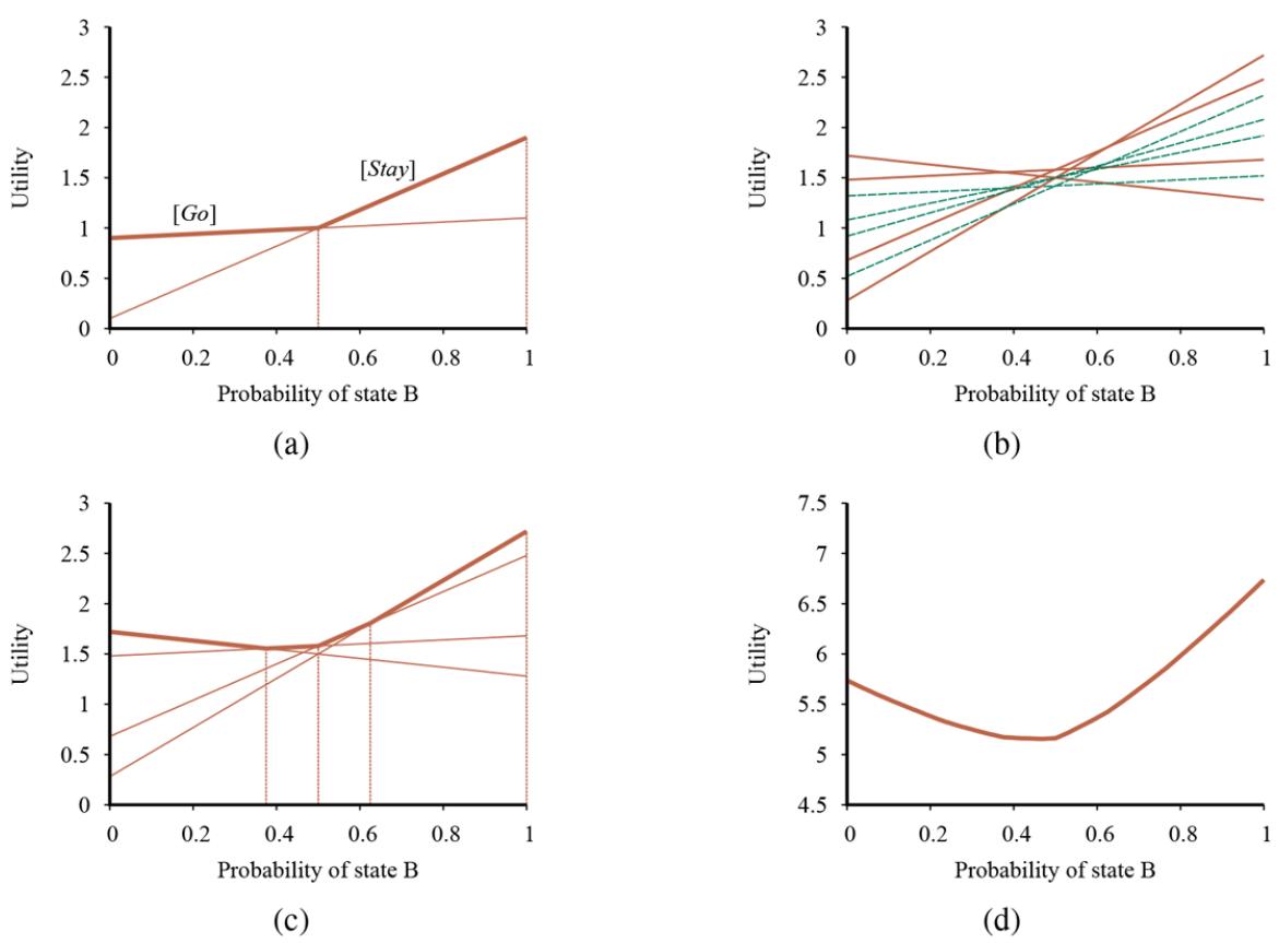
1. Utility of two one-step plans as a function of the initial belief state for the two-state world, with the corresponding utility function shown in bold. (b) Utilities for 8 distinct two-step plans. (c) Utilities for four undominated two-step plans. (d) Utility function for optimal eight-step plans.

The hyperplanes (lines, in this case) for and are shown in Figure 17.15(a) and their maximum is shown in bold. The bold line therefore represents the utility function for the finite-horizon problem that allows just one action, and in each “piece” of the piecewise linear utility function an optimal action is the first action of the corresponding conditional plan. In this case, the optimal one-step policy is to Stay when and Go otherwise.

Once we have utilities for all the conditional plans of depth 1 in each physical state , we can compute the utilities for conditional plans of depth 2 by considering each possible first action, each possible subsequent percept, and then each way of choosing a depth-1 plan to execute for each percept:

There are eight distinct depth-2 plans in all, and their utilities are shown in Figure 17.15(b) . Notice that four of the plans, shown as dashed lines, are suboptimal across the entire belief space—we say these plans are dominated, and they need not be considered further. There are four undominated plans, each of which is optimal in a specific region, as shown in Figure 17.15(c) . The regions partition the belief-state space.

Dominated plan

We repeat the process for depth 3, and so on. In general, let be a depth- conditional plan whose initial action is and whose depth- subplan for percept is ; then

(17.18)

\[\alpha\_p(s) = \sum\_{s'} P(s'|s, a)[R(s, a, s') + \gamma \sum\_e P(e|s')\alpha\_{p,e}(s')].\]

This recursion naturally gives us a value iteration algorithm, which is given in Figure 17.16 . The structure of the algorithm and its error analysis are similar to those of the basic value iteration algorithm in Figure 17.6 on page 573; the main difference is that instead of computing one utility number for each state, POMDP-VALUE-ITERATION maintains a collection of undominated plans with their utility hyperplanes.

Figure 17.16

A high-level sketch of the value iteration algorithm for POMDPs. The REMOVE-DOMINATED-PLANS step and MAX-DIFFERENCE test are typically implemented as linear programs.

The algorithm’s complexity depends primarily on how many plans get generated. Given actions and possible observations, there are distinct depth- plans. Even for the lowly two-state world with , that’s plans. The elimination of dominated plans is essential for reducing this doubly exponential growth: the number of undominated plans with is just 144. The utility function for these 144 plans is shown in Figure 17.15(d) .

Notice that the intermediate belief states have lower value than state and state , because in the intermediate states the agent lacks the information needed to choose a good action. This is why information has value in the sense defined in Section 16.6 and optimal policies in POMDPs often include information-gathering actions.

Given such a utility function, an executable policy can be extracted by looking at which hyperplane is optimal at any given belief state and executing the first action of the corresponding plan. In Figure 17.15(d) , the corresponding optimal policy is still the same as for depth-1 plans: Stay when and Go otherwise.

In practice, the value iteration algorithm in Figure 17.16 is hopelessly inefficient for larger problems—even the POMDP is too hard. The main reason is that given undominated conditional plans at level , the algorithm constructs conditional plans at level before eliminating the dominated ones. With the four-bit sensor, is 16, and can be in the hundreds, so this is hopeless.

Since this algorithm was developed in the 1970s, there have been several advances, including more efficient forms of value iteration and various kinds of policy iteration algorithms. Some of these are discussed in the notes at the end of the chapter. For general POMDPs, however, finding optimal policies is very difficult (PSPACE-hard, in fact—that is, very hard indeed). The next section describes a different, approximate method for solving POMDPs, one based on look-ahead search.

17.5.2 Online algorithms for POMDPs

The basic design for an online POMDP agent is straightforward: it starts with some prior belief state; it chooses an action based on some deliberation process centered on its current belief state; after acting, it receives an observation and updates its belief state using a filtering algorithm; and the process repeats.

One obvious choice for the deliberation process is the expectimax algorithm from Section 17.2.4 , except with belief states rather than physical states as the decision nodes in the tree. The chance nodes in the POMDP tree have branches labeled by possible observations and leading to the next belief state, with transition probabilities given by Equation (17.17) . A fragment of the belief-state expectimax tree for the POMDP is shown in Figure 17.17 .

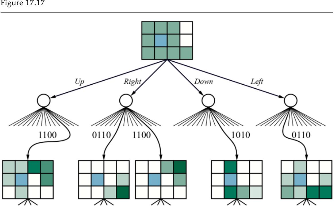
Part of an expectimax tree for the POMDP with a uniform initial belief state. The belief states are depicted with shading proportional to the probability of being in each location.

The time complexity of an exhaustive search to depth is , where is the number of available actions and is the number of possible percepts. (Notice that this is far less than the number of possible depth- conditional plans generated by value iteration.) As in the observable case, sampling at the chance nodes is a good way to cut down the branching factor without losing too much accuracy in the final decision. Thus, the complexity of approximate online decision making in POMDPs may not be drastically worse than that in MDPs.

For very large state spaces, exact filtering is infeasible, so the agent will need to run an approximate filtering algorithm such as particle filtering (see page 492). Then the belief states in the expectimax tree become collections of particles rather than exact probability distributions. For problems with long horizons, we may also need to run the kind of longrange playouts used in the UCT algorithm (Figure 5.11 ). The combination of particle filtering and UCT applied to POMDPs goes under the name of partially observable Monte Carlo planning or POMCP. With a DDN representation for the model, the POMCP algorithm is, at least in principle, applicable to very large and realistic POMDPs. Details of the algorithm are explored in Exercise 17.POMC. POMCP is capable of generating competent behavior in the POMDP. A short (and somewhat fortunate) example is shown in Figure 17.18 .

Figure 17.18

A sequence of percepts, belief states, and actions in the POMDP with a wall-sensing error of . Notice how the early Left moves are safe—they are very unlikely to fall into —and coerce the agent’s location into a small number of possible locations. After moving Up, the agent thinks it is probably in , but possibly in . Fortunately, moving Right is a good idea in both cases, so it moves Right, finds out that it had been in and is now in , and then continues moving Right and reaches the goal.

POMCP

POMDP agents based on dynamic decision networks and online decision making have a number of advantages compared with other, simpler agent designs presented in earlier chapters. In particular, they handle partially observable, stochastic environments and can easily revise their “plans” to handle unexpected evidence. With appropriate sensor models, they can handle sensor failure and can plan to gather information. They exhibit “graceful degradation” under time pressure and in complex environments, using various approximation techniques.

So what is missing? The principal obstacle to real-world deployment of such agents is the inability to generate successful behavior over long time-scales. Random or near-random playouts have no hope of gaining any positive reward on, say, the task of laying the table for dinner, which might take tens of millions of motor-control actions. It seems necessary to borrow some of the hierarchical planning ideas described in Section 11.4 . At the time of writing, there are not yet satisfactory and efficient ways to apply these ideas in stochastic, partially observable environments.

Summary

This chapter shows how to use knowledge about the world to make decisions even when the outcomes of an action are uncertain and the rewards for acting might not be reaped until many actions have passed. The main points are as follows:

• Sequential decision problems in stochastic environments, also called Markov decision processes, or MDPs, are defined by a transition model specifying the probabilistic outcomes of actions and a reward function specifying the reward in each state.
• The utility of a state sequence is the sum of all the rewards over the sequence, possibly discounted over time. The solution of an MDP is a policy that associates a decision with every state that the agent might reach. An optimal policy maximizes the utility of the state sequences encountered when it is executed.
• The utility of a state is the expected sum of rewards when an optimal policy is executed from that state. The value iteration algorithm iteratively solves a set of equations relating the utility of each state to those of its neighbors.
• Policy iteration alternates between calculating the utilities of states under the current policy and improving the current policy with respect to the current utilities.
• Partially observable MDPs, or POMDPs, are much more difficult to solve than are MDPs. They can be solved by conversion to an MDP in the continuous space of belief states; both value iteration and policy iteration algorithms have been devised. Optimal behavior in POMDPs includes information gathering to reduce uncertainty and therefore make better decisions in the future.
• A decision-theoretic agent can be constructed for POMDP environments. The agent uses a dynamic decision network to represent the transition and sensor models, to update its belief state, and to project forward possible action sequences.

We shall return MDPs and POMDPs in Chapter 22 , which covers reinforcement learning methods that allow an agent to improve its behavior from experience.

Bibliographical and Historical Notes

Richard Bellman developed the ideas underlying the modern approach to sequential decision problems while working at the RAND Corporation beginning in 1949. According to his autobiography (Bellman, 1984), he coined the term “dynamic programming” to hide from a research-phobic Secretary of Defense, Charles Wilson, the fact that his group was doing mathematics. (This cannot be strictly true, because his first paper using the term (Bellman, 1952) appeared before Wilson became Secretary of Defense in 1953.) Bellman’s book, Dynamic Programming (1957), gave the new field a solid foundation and introduced the value iteration algorithm.

Shapley (1953b) actually described the value iteration algorithm independently of Bellman, but his results were not widely appreciated in the operations research community, perhaps because they were presented in the more general context of Markov games. Although the original formulations included discounting, its analysis in terms of stationary preferences was suggested by Koopmans (1972). The shaping theorem is due to Ng et al. (1999).

Ron Howard’s Ph.D. thesis (1960) introduced policy iteration and the idea of average reward for solving infinite-horizon problems. Several additional results were introduced by Bellman and Dreyfus (1962). The use of contraction mappings in analyzing dynamic programming algorithms is due to Denardo (1967). Modified policy iteration is due to van Nunen (1976) and Puterman and Shin (1978). Asynchronous policy iteration was analyzed by Williams and Baird (1993), who also proved the policy loss bound in Equation (17.13) . The general family of prioritized sweeping algorithms aims to speed up convergence to optimal policies by heuristically ordering the value and policy update calculations (Moore and Atkeson, 1993; Andre et al., 1998; Wingate and Seppi, 2005).

The formulation of MDP-solving as a linear program is due to de Ghellinck (1960), Manne (1960), and D’Épenoux (1963). Although linear programming has traditionally been considered inferior to dynamic programming as an exact solution method for MDPs, de Farias and Roy (2003) show that it is possible to use linear programming and a linear representation of the utility function to obtain provably good approximate solutions to very large MDPs. Papadimitriou and Tsitsiklis (1987) and Littman et al. (1995) provide general results on the computational complexity of MDPs. Yinyu Ye (2011) analyzes the relationship between policy iteration and the simplex method for linear programming and proves that for fixed , the runtime of policy iteration is polynomial in the number of states and actions.

Seminal work by Sutton (1988) and Watkins (1989) on reinforcement learning methods for solving MDPs played a significant role in introducing MDPs into the AI community. (Earlier work by Werbos (1977) contained many similar ideas, but was not taken up to the same extent.) AI researchers have pushed MDPs in the direction of more expressive representations that can accommodate much larger problems than the traditional atomic representations based on transition matrices.

The basic ideas for an agent architecture using dynamic decision networks were proposed by Dean and Kanazawa (1989a). Tatman and Shachter (1990) showed how to apply dynamic programming algorithms to DDN models. Several authors made the connection between MDPs and AI planning problems, developing probabilistic forms of the compact STRIPS representation for transition models (Wellman, 1990b; Koenig, 1991). The book Planning and Control by Dean and Wellman (1991) explores the connection in great depth.

Later work on factored MDPs (Boutilier et al., 2000; Koller and Parr, 2000; Guestrin et al., 2003b) uses structured representations of the value function as well as the transition model, with provable improvements in complexity. Relational MDPs (Boutilier et al., 2001; Guestrin et al., 2003a) go one step further, using structured representations to handle domains with many related objects. Open-universe MDPs and POMDPs (Srivastava et al., 2014b) also allow for uncertainty over the existence and identity of objects and actions.

Factored MDP

Relational MDP

Many authors have developed approximate online algorithms for decision making in MDPs, often borrowing explicitly from earlier AI approaches to real-time search and game-playing

(Werbos, 1992; Dean et al., 1993; Tash and Russell, 1994). The work of Barto et al. (1995) on RTDP (real-time dynamic programming) provided a general framework for understanding such algorithms and their connection to reinforcement learning and heuristic search. The analysis of depth-bounded expectimax with sampling at chance nodes is due to Kearns et al. (2002). The UCT algorithm described in the chapter is due to Kocsis and Szepesvari (2006) and borrows from earlier work on random playouts for estimating the values of states (Abramson, 1990; Brügmann, 1993; Chang et al., 2005).

Bandit problems were introduced by Thompson (1933) but came to prominence after World War II through the work of Herbert Robbins (1952). Bradt et al. (1956) proved the first results concerning stopping rules for one-armed bandits, which led eventually to the breakthrough results of John Gittins (Gittins and Jones, 1974; Gittins, 1989). Katehakis and Veinott (1987) suggested the restart MDP as a method of computing Gittins indices. The text by Berry and Fristedt (1985) covers many variations on the basic problem, while the pellucid online text by Ferguson (2001) connects bandit problems with stopping problems.

Lai and Robbins (1985) initiated the study of the asymptotic regret of optimal bandit policies. The UCB heuristic was introduced and analyzed by Auer et al. (2002). Bandit superprocesses (BSPs) were first studied by Nash (1973) but have remained largely unknown in AI. Hadfield-Menell and Russell (2015) describe an efficient branch-and-bound algorithm capable of solving relatively large BSPs. Selection problems were introduced by Bechhofer (1954). Hay et al. (2012) developed a formal framework for metareasoning problems, showing that simple instances mapped to selection rather than bandit problems. They also proved the satisfying result that expected computation cost of the optimal computational strategy is never higher than the expected gain in decision quality—although there are cases where the optimal policy may, with some probability, keep computing long past the point where any possible gain has been used up.

The observation that a partially observable MDP can be transformed into a regular MDP over belief states is due to Astrom (1965) and Aoki (1965). The first complete algorithm for the exact solution of POMDPs—essentially the value iteration algorithm presented in this chapter—was proposed by Edward Sondik (1971) in his Ph.D. thesis. (A later journal paper by Smallwood and Sondik (1973) contains some errors, but is more accessible.) Lovejoy (1991) surveyed the first twenty-five years of POMDP research, reaching somewhat pessimistic conclusions about the feasibility of solving large problems.

The first significant contribution within AI was the Witness algorithm (Cassandra et al., 1994; Kaelbling et al., 1998), an improved version of POMDP value iteration. Other algorithms soon followed, including an approach due to Hansen (1998) that constructs a policy incrementally in the form of a finite-state automaton whose states define the possible belief states of the agent.

More recent work in AI has focused on point-based value iteration methods that, at each iteration, generate conditional plans and -vectors for a finite set of belief states rather than for the entire belief space. Lovejoy (1991) proposed such an algorithm for a fixed grid of points, an approach taken also by Bonet (2002). An influential paper by Pineau et al. (2003) suggested generating reachable points by simulating trajectories in a somewhat greedy fashion; Spaan and Vlassis (2005) observe that one need generate plans for only a small, randomly selected subset of points to improve on the plans from the previous iteration for all points in the set. Shani et al. (2013) survey these and other developments in point-based algorithms, which have led to good solutions for problems with thousands of states. Because POMDPs are PSPACE-hard (Papadimitriou and Tsitsiklis, 1987), further progress on offline solution methods may require taking advantage of various kinds of structure in value functions arising from a factored representation of the model.

The online approach for POMDPs—using look-ahead search to select an action for the current belief state—was first examined by Satia and Lave (1973). The use of sampling at chance nodes was explored analytically by Kearns et al. (2000) and Ng and Jordan (2000). The POMCP algorithm is due to Silver and Veness (2011).

With the development of reasonably effective approximation algorithms for POMDPs, their use as models for real-world problems has increased, particularly in education (Rafferty et al., 2016), dialog systems (Young et al., 2013), robotics (Hsiao et al., 2007; Huynh and Roy, 2009), and self-driving cars (Forbes et al., 1995; Bai et al., 2015). An important large-scale application is the Airborne Collision Avoidance System X (ACAS X), which keeps airplanes and drones from colliding midair. The system uses POMDPs with neural networks to do function approximation. ACAS X significantly improves safety compared to the legacy TCAS system, which was built in the 1970s using expert system technology (Kochenderfer, 2015; Julian et al., 2018).

Complex decision making has also been studied by economists and psychologists. They find that decision makers are not always rational, and may not be operating exactly as described by the models in this chapter. For example, when given a choice, a majority of people prefer $100 today over a guarantee of $200 in two years, but those same people prefer $200 in eight years over $100 in six years. One way to interpret this result is that people are not using additive exponentially discounted rewards; perhaps they are using hyperbolic rewards (the hyperbolic function dips more steeply in the near term than does the exponential decay function). This and other possible interpretations are discussed by Rubinstein (2003).

Hyperbolic reward

The texts by Bertsekas (1987) and Puterman (1994) provide rigorous introductions to sequential decision problems and dynamic programming. Bertsekas and Tsitsiklis (1996) include coverage of reinforcement learning. Sutton and Barto (2018) cover similar ground but in a more accessible style. Sigaud and Buffet (2010), Mausam and Kolobov (2012) and Kochenderfer (2015) cover sequential decision making from an AI perspective. Krishnamurthy (2016) provides thorough coverage of POMDPs.

Chapter 18 Multiagent Decision Making

In which we examine what to do when more than one agent inhabits the environment.

18.1 Properties of Multiagent Environments

So far, we have largely assumed that only one agent has been doing the sensing, planning, and acting. But this represents a huge simplifying assumption, which fails to capture many real-world AI settings. In this chapter, therefore, we will consider the issues that arise when an agent must make decisions in environments that contain multiple actors. Such environments are called multiagent systems, and agents in such a system face a multiagent planning problem. However, as we will see, the precise nature of the multiagent planning problem—and the techniques that are appropriate for solving it—will depend on the relationships among the agents in the environment.

Multiagent systems

Multiagent planning problem

18.1.1 One decision maker

The first possibility is that while the environment contains multiple actors, it contains only one decision maker. In such a case, the decision maker develops plans for the other agents, and tells them what to do. The assumption that agents will simply do what they are told is called the benevolent agent assumption. However, even in this setting, plans involving multiple actors will require actors to synchronize their actions. Actors and will have to act at the same time for joint actions (such as singing a duet), at different times for mutually exclusive actions (such as recharging batteries when there is only one plug), and sequentially when one establishes a precondition for the other (such as washing the dishes and then drying them).

Benevolent agent assumption

One special case is where we have a single decision maker with multiple effectors that can operate concurrently—for example, a human who can walk and talk at the same time. Such an agent needs to do multieffector planning to manage each effector while handling positive and negative interactions among the effectors. When the effectors are physically decoupled into detached units—as in a fleet of delivery robots in a factory—multieffector planning becomes multibody planning.

Multieffector planning

Multibody planning

A multibody problem is still a “standard” single-agent problem as long as the relevant sensor information collected by each body can be pooled—either centrally or within each body—to form a common estimate of the world state that then informs the execution of the overall plan; in this case, the multiple bodies can be thought of as acting as a single body. When communication constraints make this impossible, we have what is sometimes called a decentralized planning problem; this is perhaps a misnomer, because the planning phase is centralized but the execution phase is at least partially decoupled. In this case, the subplan constructed for each body may need to include explicit communicative actions with other bodies. For example, multiple reconnaissance robots covering a wide area may often be out of radio contact with each other and should share their findings during times when communication is feasible.

Decentralized planning

18.1.2 Multiple decision makers

The second possibility is that the other actors in the environment are also decision makers: they each have preferences and choose and execute their own plan. We call them counterparts. In this case, we can distinguish two further possibilities.

The first is that, although there are multiple decision makers, they are all pursuing a common goal. This is roughly the situation of workers in a company, in which different decision makers are pursuing, one hopes, the same goals on behalf of the company. The main problem faced by the decision makers in this setting is the coordination problem: they need to ensure that they are all pulling in the same direction, and not accidentally fouling up each other’s plans.

Common goal

Coordination problem

The second possibility is that the decision makers each have their own personal preferences, which they each will pursue to the best of their abilities. It could be that the preferences are diametrically opposed, as is the case in zero-sum games such as chess (see Chapter 5 ). But most multiagent encounters are more complicated than that, with more complex preferences.

Counterparts

When there are multiple decision makers, each pursuing their own preferences, an agent must take into account the preferences of other agents, as well as the fact that these other agents are also taking into account the preferences of other agents, and so on. This brings us into the realm of game theory: the theory of strategic decision making. It is this strategic aspect of reasoning—players each taking into account how other players may act—that distinguishes game theory from decision theory. In the same way that decision theory provides the theoretical foundation for decision making in single-agent AI, game theory provides the theoretical foundation for decision making in multiagent systems.

Game theory

The use of the word “game” here is also not ideal: a natural inference is that game theory is mainly concerned with recreational pursuits, or artificial scenarios. Nothing could be further from the truth. Game theory is the theory of strategic decision making. It is used in decision making situations including the auctioning of oil drilling rights and wireless frequency spectrum rights, bankruptcy proceedings, product development and pricing decisions, and national defense—situations involving billions of dollars and many lives. Game theory in AI can be used in two main ways:

Strategic decision making

1. AGENT DESIGN: Game theory can be used by an agent to analyze its possible decisions and compute the expected utility for each of these (under the assumption that other agents are acting rationally, according to game theory). In this way, gametheoretic techniques can determine the best strategy against a rational player and the expected return for each player.

Agent design

2. MECHANISM DESIGN: When an environment is inhabited by many agents, it might be possible to define the rules of the environment (i.e., the game that the agents must play) so that the collective good of all agents is maximized when each agent adopts the game-theoretic solution that maximizes its own utility. For example, game theory can help design the protocols for a collection of Internet traffic routers so that each router has an incentive to act in such a way that global throughput is maximized. Mechanism design can also be used to construct intelligent multiagent systems that solve complex problems in a distributed fashion.

Mechanism design

Game theory provides a range of different models, each with its own set of underlying assumptions; it is important to choose the right model for each setting. The most important distinction is whether we should consider it a cooperative game or not:

In a cooperative game, it is possible to have a binding agreement between agents, thereby enabling robust cooperation. In the human world, legal contracts and social norms help establish such binding agreements. In the world of computer programs, it may be possible to inspect source code to make sure it will follow an agreement. We use cooperative game theory to analyze this situation.

Cooperative game

If binding agreements are not possible, we have a non-cooperative game. Although this term suggests that the game is inherently competitive, and that cooperation is not possible, that need not be the case: non-cooperative simply means that there is no central agreement that binds all agents and guarantees cooperation. But it could well be that agents independently decide to cooperate, because it is in their own best interests. We use non-cooperative game theory to analyze this situation.

Non-cooperative game

Some environments will combine multiple different dimensions. For example, a package delivery company may do centralized, offline planning for the routes of its trucks and planes each day, but leave some aspects open for autonomous decisions by drivers and pilots who can respond individually to traffic and weather situations. Also, the goals of the company and its employees are brought into alignment, to some extent, by the payment of incentives (salaries and bonuses)—a sure sign that this is a true multiagent system.

Incentive

18.1.3 Multiagent planning

For the time being, we will treat the multieffector, multibody, and multiagent settings in the same way, labeling them generically as multiactor settings, using the generic term actor to cover effectors, bodies, and agents. The goal of this section is to work out how to define transition models, correct plans, and efficient planning algorithms for the multiactor setting. A correct plan is one that, if executed by the actors, achieves the goal. (In the true multiagent setting, of course, the agents may not agree to execute any particular plan, but at least they will know what plans would work if they did agree to execute them.)

Multiactor

Actor

A key difficulty in attempting to come up with a satisfactory model of multiagent action is that we must somehow deal with the thorny issue of concurrency, by which we simply mean that the plans of each agent may be executed simultaneously. If we are to reason about the execution of multiactor plans, then we will first need a model of multiactor plans that embodies a satisfactory model of concurrent action.

Concurrency

In addition, multiactor action raises a whole set of issues that are not a concern in singleagent planning. In particular, agents must take into account the way in which their own actions interact with the actions of other agents. For example, an agent will need to consider whether the actions performed by other agents might clobber the preconditions of its own actions, whether the resources it makes use of while executing its policy are sharable, or may be depleted by other agents; whether actions are mutually exclusive; and a helpfully inclined agent could consider how its actions might facilitate the actions of others.

To answer these questions we need a model of concurrent action within which we can properly formulate them. Models of concurrent action have been a major focus of research in the mainstream computer science community for decades, but no definitive, universally accepted model has prevailed. Nevertheless, the following three approaches have become widely established.

The first approach is to consider the interleaved execution of the actions in respective plans. For example, suppose we have two agents, and with plans as follows:

\[\begin{array}{rcl} A &:& [a\_1, a\_2] \\ B &:& [b\_1, b\_2] .\end{array}\]

Interleaved execution

The key idea of the interleaved execution model is that the only thing we can be certain about in the execution of the two agents’ plans is that the order of actions in the respective plans will be preserved. If we further assume that actions are atomic, then there are six different ways in which the two plans above might be executed concurrently:

\[\begin{aligned} & [a\_1, a\_2, b\_1, b\_2] \\ & [b\_1, b\_2, a\_1, a\_2] \\ & [a\_1, b\_1, a\_2, b\_2] \\ & [b\_1, a\_1, b\_2, a\_2] \\ & [a\_1, b\_1, b\_2, a\_2] \\ & [b\_1, a\_1, a\_2, b\_2] \end{aligned}\]

For a plan to be correct in the interleaved execution model, it must be correct with respect to all possible interleavings of the plans. The interleaved execution model has been widely adopted within the concurrency community, because it is a reasonable model of the way multiple threads take turns running on a single CPU. However, it does not model the case where two actions actually happen at the same time. Furthermore, the number of interleaved sequences will grow exponentially with the number of agents and actions: as a consequence, checking the correctness of a plan, which is computationally straightforward in single-agent settings, is computationally difficult with the interleaved execution model.

The second approach is true concurrency, in which we do not attempt to create a full serialized ordering of the actions, but leave them partially ordered: we know that will occur before but with respect to the ordering of and for example, we can say nothing; one may occur before the other, or they could occur concurrently. We can always “flatten” a partial-order model of concurrent plans into an interleaved model, but in doing so, we lose the partial-order information. While partial-order models are arguably more satisfying than interleaved models as a theoretical account of concurrent action, they have not been as widely adopted in practice.

True concurrency

The third approach is to assume perfect synchronization: there is a global clock that each agent has access to, each action takes the same amount of time, and actions at each point in the joint plan are simultaneous. Thus, the actions of each agent are executed synchronously, in lockstep with each other (it may be that some agents execute a no-op action when they are waiting for other actions to complete). Synchronous execution is not a very complete model of concurrency in the real world, but it has a simple semantics, and for this reason, it is the model we will work with here.

Synchronization

We begin with the transition model; for the single-agent deterministic case, this is the function which gives the state that results from performing the action when the environment is in state In the single-agent setting, there might be different choices for the action; can be quite large, especially for first-order representations with many objects to act on, but action schemas provide a concise representation nonetheless.

In the multiactor setting with actors, the single action is replaced by a joint action where is the action taken by the th actor. Immediately, we see two problems: first, we have to describe the transition model for different joint actions; second, we have a joint planning problem with a branching factor of

Joint action

Having put the actors together into a multiactor system with a huge branching factor, the principal focus of research on multiactor planning has been to decouple the actors to the extent possible, so that (ideally) the complexity of the problem grows linearly with rather than exponentially with

If the actors have no interaction with one another—for example, actors each playing a game of solitaire—then we can simply solve separate problems. If the actors are loosely coupled, can we attain something close to this exponential improvement? This is, of course, a central question in many areas of AI. We have seen successful solution methods for loosely coupled systems in the context of CSPs, where “tree like” constraint graphs yielded efficient solution methods (see page 202), as well as in the context of disjoint pattern databases (page 100) and additive heuristics for planning (page 356).

Loosely coupled

The standard approach to loosely coupled problems is to pretend the problems are completely decoupled and then fix up the interactions. For the transition model, this means writing action schemas as if the actors acted independently.

Joint plan

Let’s see how this works for a game of doubles tennis. Here, we have two human tennis players who form a doubles team with the common goal of winning the match against an opponent team. Let’s suppose that at one point in the game, the team has the goal of returning the ball that has been hit to them and ensuring that at least one of them is covering the net. Figure 18.1 shows the initial conditions, goal, and action schemas for this problem. It is easy to see that we can get from the initial conditions to the goal with a twostep joint plan that specifies what each player has to do: should move over to the right baseline and hit the ball, while should just stay put at the net:

The doubles tennis problem. Two actors, and are playing together and can be in one of four locations: LeftBaseline, RightBaseline, LeftNet, and RightNet. The ball can be returned only if a player is in the right place. The NoOp action is a dummy, which has no effect. Note that each action must include the actor as an argument.

Problems arise, however, when a plan dictates that both agents hit the ball at the same time. In the real world, this won’t work, but the action schema for Hit says that the ball will be returned successfully. The difficulty is that preconditions constrain the state in which an action by itself can be executed successfully, but do not constrain other concurrent actions that might mess it up.

We solve this problem by augmenting action schemas with one new feature: a concurrent action constraint stating which actions must or must not be executed concurrently. For example, the Hit action could be described as follows:

Concurrent action constraint

In other words, the Hit action has its stated effect only if no other Hit action by another agent occurs at the same time. (In the SATPLAN approach, this would be handled by a partial action exclusion axiom.) For some actions, the desired effect is achieved only when another action occurs concurrently. For example, two agents are needed to carry a cooler full of beverages to the tennis court:

With these kinds of action schemas, any of the planning algorithms described in Chapter 11 can be adapted with only minor modifications to generate multiactor plans. To the extent that the coupling among subplans is loose—meaning that concurrency constraints come into play only rarely during plan search—one would expect the various heuristics derived for single-agent planning to also be effective in the multiactor context.

18.1.4 Planning with multiple agents: Cooperation and coordination

Now let us consider a true multiagent setting in which each agent makes its own plan. To start with, let us assume that the goals and knowledge base are shared. One might think that this reduces to the multibody case—each agent simply computes the joint solution and executes its own part of that solution. Alas, the “the” in “the joint solution” is misleading. Here is a second plan that also achieves the goal:

\[\begin{array}{rcl} \text{PLAN 2:} & A: & [Go(A, LeftNet), NoOp(A)] \\ & B: & [Go(B, RightBase), Hit(B, Ball)]. \end{array}\]

If both agents can agree on either plan 1 or plan 2, the goal will be achieved. But if chooses plan 2 and chooses plan 1, then nobody will return the ball. Conversely, if chooses 1 and chooses 2, then they will both try to hit the ball and that too will fail. The agents know this, but how can they coordinate to make sure they agree on the plan?

One option is to adopt a convention before engaging in joint activity. A convention is any constraint on the selection of joint plans. For example, the convention “stick to your side of the court” would rule out plan 1, causing both partners to select plan 2. Drivers on a road face the problem of not colliding with each other; this is (partially) solved by adopting the convention “stay on the right-hand side of the road” in most countries; the alternative, “stay on the left-hand side,” works equally well as long as all agents in an environment agree. Similar considerations apply to the development of human language, where the important thing is not which language each individual should speak, but the fact that a community all speaks the same language. When conventions are widespread, they are called social laws.

Convention

Social law

In the absence of a convention, agents can use communication to achieve common knowledge of a feasible joint plan. For example, a tennis player could shout “Mine!” or “Yours!” to indicate a preferred joint plan. Communication does not necessarily involve a verbal exchange. For example, one player can communicate a preferred joint plan to the other simply by executing the first part of it. If agent heads for the net, then agent is obliged to go back to the baseline to hit the ball, because plan 2 is the only joint plan that begins with ’s heading for the net. This approach to coordination, sometimes called plan recognition, works when a single action (or short sequence of actions) by one agent is enough for the other to determine a joint plan unambiguously.

Plan recognition

18.2 Non-Cooperative Game Theory

We will now introduce the key concepts and analytical techniques of game theory—the theory that underpins decision making in multiagent environments. Our tour will start with non-cooperative game theory.

18.2.1 Games with a single move: Normal form games

The first game model we will look at is one in which all players take action simultaneously and the result of the game is based on the profile of actions that are selected in this way. (Actually, it is not crucial that the actions take place at the same time; what matters is that no player has knowledge of the other players’ choices.) These games are called normal form games. A normal form game is defined by three components:

Normal form game

Player

• Players or agents who will be making decisions. Two-player games have received the most attention, although -player games for are also common. We give players capitalized names, like Ali and Bo or and
• Actions that the players can choose. We will give actions lowercase names, like or testify. The players may or may not have the same set of actions available.
• A payoff function that gives the utility to each player for each combination of actions by all the players. For two-player games, the payoff function for a player can be represented by a matrix in which there is a row for each possible action of one player, and a column for each possible choice of the other player: a chosen row and a chosen column define a matrix cell, which is labeled with the payoff for the relevant player. In the two-player

case, it is conventional to combine the two matrices into a single payoff matrix, in which each cell is labeled with payoffs for both players.

Payoff function

Payoff matrix

To illustrate these ideas, let’s look at an example game, called two-finger Morra. In this game, two players, and simultaneously display one or two fingers. Let the total number of fingers displayed be If is odd, collects dollars from and if is even, collects dollars from The payoff matrix for two-finger Morra is as follows: 1

1 Morra is a recreational version of an inspection game. In such games, an inspector chooses a day to inspect a facility (such as a restaurant or a biological weapons plant), and the facility operator chooses a day to hide all the nasty stuff. The inspector wins if the days are different, and the facility operator wins if they are the same.

	O: one	O: two
E: one		E = +2,0 = - 2 E = - 3,0 = + 3
E: two		E = - 3.0 = +3 E = +4.0 = - 4

We say that is the row player and is the column player. So, for example, the lowerright corner shows that when player chooses action two and also chooses two, the payoff is for and for

Row player

Column player

Before analyzing two-finger Morra, it is worth considering why game-theoretic ideas are needed at all: why can’t we tackle the challenge facing (say) player using the apparatus of decision theory and utility maximization that we’ve been using elsewhere in the book? To see why something else is needed, let’s suppose is trying to find the best action to perform. The alternatives are one or two. If chooses one, then the payoff will be either or Which payoff will actually receive, however, will depend on the choice made by the most that can do, as the row player, is to force the outcome of the game to be in a particular row. Similarly, chooses only the column.

To choose optimally between these possibilities, must take into account how will act as a rational decision maker. But in turn, should take into account the fact that is a rational decision maker. Thus, decision making in multiagent settings is quite different in character to decision making in single-agent settings, because the players need to take each other’s reasoning into account. The role of solution concepts in game theory is to try to make this kind of reasoning precise.

Solution concept

The term strategy is used in game theory to denote what we have previously called a policy. A pure strategy is a deterministic policy; for a single-move game, a pure strategy is just a single action. As we will see below, for many games an agent can do better with a mixed strategy, which is a randomized policy that selects actions according to a probability distribution. The mixed strategy that chooses action with probability and action otherwise is written For example, a mixed strategy for two-finger Morra might be A strategy profile is an assignment of a strategy to each player; given the strategy profile, the game’s outcome is a numeric value for each player—if players use mixed strategies, then we must use expected utility.

Strategy

Pure strategy

Mixed strategy

Strategy profile

So, how should agents decide act in games like Morra? Game theory provides a range of solution concepts that attempt to define rational action with respect to an agent’s beliefs about the other agent’s beliefs. Unfortunately, there is no one perfect solution concept: it is problematic to define what “rational” means when each agent chooses only part of the strategy profile that determines the outcome.

Prisoner’s dilemma

We introduce our first solution concept through what is probably the most famous game in the game theory canon—the prisoner’s dilemma. This game is motivated by the following story: Two alleged burglars, Ali and Bo, are caught red-handed near the scene of a burglary and are interrogated separately. A prosecutor offers each a deal: if you testify against your partner as the leader of a burglary ring, you’ll go free for being the cooperative one, while your partner will serve 10 years in prison. However, if you both testify against each other, you’ll both get years. Ali and Bo also know that if both refuse to testify they will serve only year each for the lesser charge of possessing stolen property. Now Ali and Bo face the socalled prisoner’s dilemma: should they testify or refuse? Being rational agents, Ali and Bo each want to maximize their own expected utility, which means minimizing the number of years in prison—each is indifferent about the welfare of the other player. The prisoner’s dilemma is captured in the following payoff matrix:

	Ali:testify	Ali:refuse
Bo:testify	A = - 5.B = - 5	A = - 10.B = 0
Bo:refuse	A = 0.B = - 10	A = - 1.B = - 1

Now, put yourself in Ali’s place. She can analyze the payoff matrix as follows:

• Suppose Bo plays testify. Then I get 5 years if I testify and 10 years if I don’t, so in that case testifying is better.
• On the other hand, if Bo plays refuse, then I go free if I testify and I get 1 year if I refuse, so testifying is also better in that case.
• So no matter what Bo chooses to do, it would be better for me to testify.

Ali has discovered that testify is a dominant strategy for the game. We say that a strategy for player strongly dominates strategy if the outcome for is better for than the outcome for for every choice of strategies by the other player(s). Strategy weakly dominates if is better than on at least one strategy profile and no worse on any other. A dominant strategy is a strategy that dominates all others. A common assumption in game theory is that a rational player will always choose a dominant strategy and avoid a dominated strategy. Being rational—or at least not wishing to be thought irrational—Ali chooses the dominant strategy.

Dominant strategy

Strong domination

Weak domination

It is not hard to see that Bo’s reasoning will be identical: he will also conclude that testify is a dominant strategy for him, and will choose to play it. The solution of the game, according to dominant strategy analysis, will be that both players choose testify, and as a consequence both will serve 5 years in prison.

In a situation like this, where all players choose a dominant strategy, then the outcome that results is said to be a dominant strategy equilibrium. It is an “equilibrium” because no player has any incentive to deviate from their part of it: by definition, if they did so, they could not do better, and may do worse. In this sense, dominant strategy equilibrium is a very strong solution concept.

Dominant strategy equilibrium

Going back to the prisoner’s dilemma, we can see that the dilemma is that the dominant strategy equilibrium outcome in which both players testify is worse for both players than the outcome they would get if they both refused to testify. The (refuse, refuse) outcome would give both players just one year in prison, which would be better for both of them than the 5 years that each would serve if they chose the dominant strategy equilibrium.

Is there any way for Ali and Bo to arrive at the (refuse, refuse) outcome? It is certainly an allowable option for both of them to refuse to testify, but it is hard to see how rational agents could make this choice, given the way the game is set up. Remember, this is a noncooperative game: they aren’t allowed to talk to each other, so they cannot make a binding agreement to refuse.

It is, however, possible to get to the (refuse, refuse) solution if we change the game. We could change it to a cooperative game where the agents are allowed to form a binding agreement. Or we could change to a repeated game in which the players know that they will meet again—we will see how this works below. Alternatively, the players might have moral beliefs that encourage cooperation and fairness. But that would mean they have different utility functions, and again, they would be playing a different game.

The presence of a dominant strategy for a particular player greatly simplifies the decision making process for that player. Once Ali has realized that testifying is a dominant strategy, she doesn’t need to invest any effort in trying to figure out what Bo will do, because she knows that no matter what Bo does, testifying would be her best response. However, most games have neither dominant strategies nor dominant strategy equilibria. It is rare that a single strategy is the best response to all possible counterpart strategies.

Best response

The next solution concept we consider is weaker than dominant strategy equilibrium, but it is much more widely applicable. It is called Nash equilibrium, and is named for John Forbes Nash, Jr. (1928–2015), who studied it in his 1950 Ph.D. thesis—work for which he was awarded a Nobel Prize in 1994.

Nash equilibrium

A strategy profile is a Nash equilibrium if no player could unilaterally change their strategy and as a consequence receive a higher payoff, under the assumption that the other players stayed with their strategy choices. Thus, in a Nash equilibrium, every player is simultaneously playing a best response to the choices of their counterparts. A Nash equilibrium represents a stable point in a game: stable in the sense that there is no rational incentive for any player to deviate. However, Nash equilibria are local stable points: as we will see, a game may contain multiple Nash equilibria.

Since a dominant strategy is a best response to all counterpart strategies, it follows that any dominant strategy equilibrium must also be a Nash equilibrium (Exercise 18.EQIB). In the prisoner’s dilemma, therefore, there is a unique dominant strategy equilibrium, which is also the unique Nash equilibrium.

The following example game demonstrates, first, that sometimes games have no dominant strategies, and second, that some games have multiple Nash equilibria.

	Ali:l	Ali:r
Bo:t	A = 10. B = 10	A = 0.B = 0
Bo:b	A = 0.B = 0	A = 1, B = 1

It is easy to verify that there are no dominant strategies in this game, for either player, and hence no dominant strategy equilibrium. However, the strategy profiles and are both Nash equilibria. Now, clearly it is in the interests of both agents to aim for the same Nash equilibrium—either or —but since we are in the domain of non-cooperative game theory, players must make their choices independently, without any knowledge of the choices of the others, and without any way of making an agreement with them. This is an example of a coordination problem: the players want to coordinate their actions globally, so that they both choose actions leading to the same equilibrium, but must do so using only local decision making.

Focal point

A number of approaches to resolving coordination problems have been proposed. One idea is that of focal points. A focal point in a game is an outcome that in some way stands out to players as being an “obvious” outcome upon which to coordinate their choices. This is of course not a precise definition—what it means will depend on the game at hand. In the example above, though, there is one obvious focal point: the outcome would give both players substantially higher utility than they would obtain if they coordinated on From the point of view of game theory, both outcomes are Nash equilibria—but it would be a perverse player indeed who expected to coordinate on

Some games have no Nash equilibria in pure strategies, as the following game, called matching pennies, illustrates. In this game, Ali and Bo simultaneously choose one side of a coin, either heads of tails: if they make the same choices, then Bo gives Ali $1, while if they make different choices, then Ali gives Bo $1:

	Ali:heads	Alitails
Bo:heads	A=1.B=-1	A = - 1.B = 1
Bo:tails	A = - 1.B = 1	A=1,B=-1

Matching pennies

We invite the reader to check that the game contains no dominant strategies, and that no outcome is a Nash equilibrium in pure strategies: in every outcome, one player regrets their choice, and would rather have chosen differently, given the choice of the other player.

To find a Nash equilibrium, the trick is to use mixed strategies—to allow players to randomize over their choices. Nash proved that every game has at least one Nash equilibrium in mixed strategies. This explains why Nash equilibrium is such an important solution concept: other solution concepts, such as dominant strategy equilibrium, are not guaranteed to exist for every game, but we always get a solution if we look for Nash equilibria with mixed strategies.

In the case of matching pennies, we have a Nash equilibrium in mixed strategies if both players choose heads and tails with equal probability. To see that this outcome is indeed a Nash equilibrium, suppose one of the players chose an outcome with a probability other than Then the other player would be able to exploit that, putting all their weight behind a particular strategy. For example, suppose Bo played heads with probability (and so tails with probability ). Then Ali would do best to play heads with certainty. It is then easy to see that Bo playing heads with probability could not form part of any Nash equilibrium.

18.2.2 Social welfare

The main perspective in game theory is that of players within the game, trying to obtain the best outcomes for themselves that they can. However, it is sometimes instructive to adopt a different perspective. Suppose you were a benevolent, omniscient entity looking down on the game, and you were able to choose the outcome. Being benevolent, you want to choose the best overall outcome—the outcome that would be best for society as a whole, so to speak. How should you choose? What criteria might you apply? This is where the notion of social welfare comes in.

Social welfare

Probably the most important and least contentious social welfare criterion is that you should avoid outcomes that waste utility. This requirement is captured in the concept of Pareto optimality, which is named for the Italian economist Vilfredo Pareto (1848–1923). An outcome is Pareto optimal if there is no other outcome that would make one player better off without making someone else worse off. If you choose an outcome that is not Pareto optimal, then it wastes utility in the sense that you could have given more utility to at least one agent, without taking any from other agents.

Pareto optimality

Utilitarian social welfare is a measure of how good an outcome is in the aggregate. The utilitarian social welfare of an outcome is simply the sum of utilities given to players by that outcome. There are two key difficulties with utilitarian social welfare. The first is that it considers the sum but not the distribution of utilities among players, so it could lead to a very unequal distribution if that happens to maximize the sum. The second difficulty is that it assumes a common scale for utilities. Many economists argue that this is impossible to establish because utility (unlikely money) is a subjective quantity. If we’re trying to decide how to divide up a batch of cookies, should we give them all to the utility monster who says, “I love cookies a thousand times more than anyone else?” That would maximize the total self-reported utility, but doesn’t seem right.

Utilitarian social welfare

The question of how utility is distributed among players is addressed by research in egalitarian social welfare. For example, one proposal suggests that we should maximize the expected utility of the worst-off member of society—a maximin approach. Other metrics are possible, including the Gini coefficient, which summarizes how evenly utility is spread among the players. The main difficulties with such proposals is that they may sacrifice a great deal of total welfare for small distributional gains, and, like plain utilitarianism, they are still at the mercy of the utility monster.

Egalitarian social welfare

Gini coefficient

Applying these concepts to the prisoner’s dilemma game, introduced above, explains why it is called a dilemma. Recall that (testify, testify) is a dominant strategy equilibrium, and the only Nash equilibrium. However, this is the only outcome that is not Pareto optimal. The outcome (refuse, refuse) maximizes both utilitarian and egalitarian social welfare. The dilemma in the prisoner’s dilemma thus arises because a very strong solution concept (dominant strategy equilibrium) leads to an outcome that essentially fails every test of what counts as a reasonable outcome from the point of view of the “society.” Yet there is no clear way for the individual players to arrive at a better solution.

Computing equilibria

Let’s now consider the key computational questions associated with the concepts discussed above. First we will consider pure strategies, where randomization is not permitted.

If players have only a finite number of possible choices, then exhaustive search can be used to find equilibria: iterate through each possible strategy profile, and check whether any player has a beneficial deviation from that profile; if not, then it is a Nash equilibrium in pure strategies. Dominant strategies and dominant strategy equilibria can be computed by

similar algorithms. Unfortunately, the number of possible strategy profiles for players each with possible actions, is i.e., infeasibly large for an exhaustive search.

An alternative approach, which works well in some games, is myopic best response (also known as iterated best response): start by choosing a strategy profile at random; then, if some player is not playing their optimal choice given the choices of others, flip their choice to an optimal one, and repeat the process. The process will converge if it leads to a strategy profile in which every player is making an optimal choice, given the choices of the others—a Nash equilibrium, in other words. For some games, myopic best response does not converge, but for some important classes of games, it is guaranteed to converge.

Myopic best response

Computing mixed-strategy equilibria is algorithmically much more intricate. To keep things simple, we will focus on methods for zero-sum games and comment briefly on their extension to other games at the end of this section.

In 1928, von Neumann developed a method for finding the optimal mixed strategy for twoplayer, zero-sum games—games in which the payoffs always add up to zero (or a constant, as explained on page 147). Clearly, Morra is such a game. For two-player, zero-sum games, we know that the payoffs are equal and opposite, so we need consider the payoffs of only one player, who will be the maximizer (just as in Chapter 5 ). For Morra, we pick the even player to be the maximizer, so we can define the payoff matrix by the values —the payoff to if does and does (For convenience we call player “her” and “him.”) Von Neumann’s method is called the maximin technique, and it works as follows:

Zero-sum game

• Suppose we change the rules as follows: first picks her strategy and reveals it to Then picks his strategy, with knowledge of ’s strategy. Finally, we evaluate the expected payoff of the game based on the chosen strategies. This gives us a turn-taking game to which we can apply the standard minimax algorithm from Chapter 5 . Let’s suppose this gives an outcome Clearly, this game favors so the true utility of the original game (from ’s point of view) is at least For example, if we just look at pure strategies, the minimax game tree has a root value of (see Figure 18.2(a) ), so we know that
• Now suppose we change the rules to force to reveal his strategy first, followed by Then the minimax value of this game is and because this game favors we know that is at most With pure strategies, the value is (see Figure 18.2(b) ), so we know

Figure 18.2

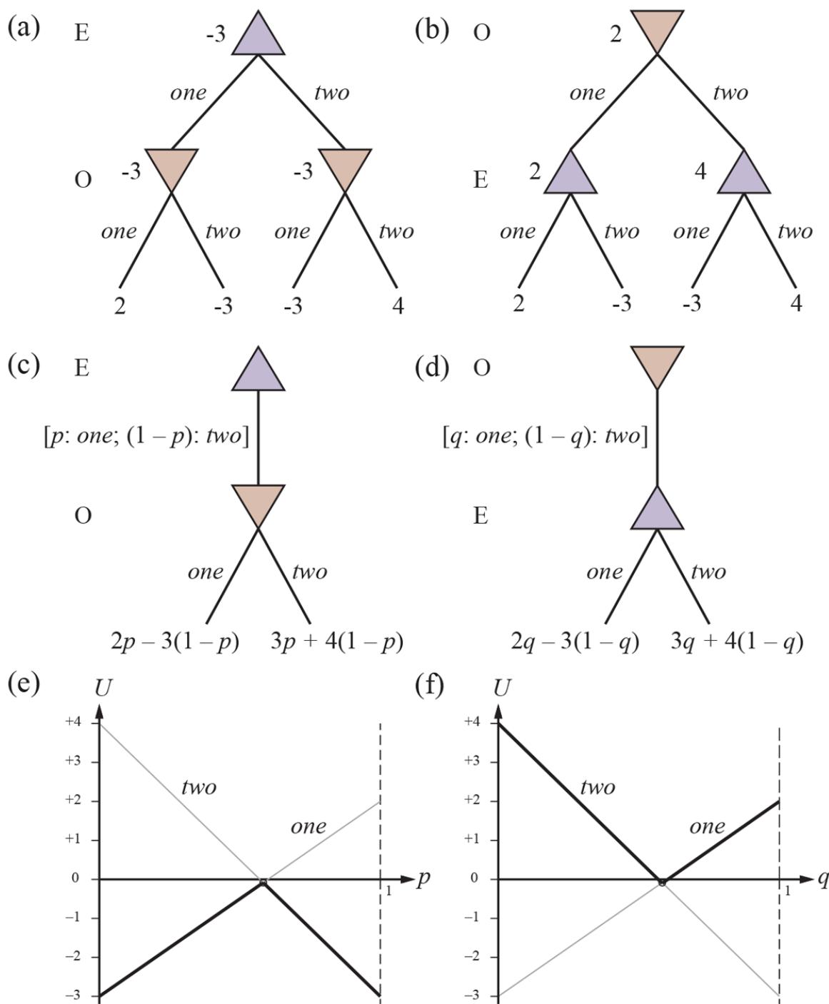
1. and (b): Minimax game trees for two-finger Morra if the players take turns playing pure strategies. (c) and (d): Parameterized game trees where the first player plays a mixed strategy. The payoffs depend on the probability parameter ( or ) in the mixed strategy. (e) and (f): For any particular value of the probability parameter, the second player will choose the “better” of the two actions, so the value of the first player’s mixed strategy is given by the heavy lines. The first player will choose the probability parameter for the mixed strategy at the intersection point.

Combining these two arguments, we see that the true utility of the solution to the original game must satisfy

\[U\_{E,O} \le U \le U\_{O,E} \qquad \text{or in this case}, \qquad -3 \le U \le 2.1\]

To pinpoint the value of we need to turn our analysis to mixed strategies. First, observe the following: once the first player has revealed a strategy, the second player might as well choose a pure strategy. The reason is simple: if the second player plays a mixed strategy, its expected utility is a linear combination of the utilities of the pure strategies, and This linear combination can never be better than the better of and so the second player can just choose the better one.

With this observation in mind, the minimax trees can be thought of as having infinitely many branches at the root, corresponding to the infinitely many mixed strategies the first player can choose. Each of these leads to a node with two branches corresponding to the pure strategies for the second player. We can depict these infinite trees finitely by having one “parameterized” choice at the root:

If chooses first, the situation is as shown in Figure 18.2(c) . chooses the strategy at the root, and then chooses a pure strategy (and hence a move) given the value of If chooses one, the expected payoff (to ) is if chooses two, the expected payoff is We can draw these two payoffs as straight lines on a graph, where ranges from 0 to 1 on the -axis, as shown in Figure 18.2(e) . the minimizer, will always choose the lower of the two lines, as shown by the heavy lines in the figure. Therefore, the best that can do at the root is to choose to be at the intersection point, which is where

\[5p - 3 = 4 - 7p \qquad \Rightarrow \qquad p = 7/12.1\]

The utility for at this point is

If moves first, the situation is as shown in Figure 18.2(d) . chooses the strategy at the root, and then chooses a move given the value of The payoffs are and Again, Figure 18.2(f) shows that the best can do at the root is to choose the intersection point: 2

\[5q - 3 = 4 - 7q \qquad \Rightarrow \qquad q = 7/12.\]

2 It is a coincidence that these equations are the same as those for the coincidence arises because This also explains why the optimal strategy is the same for both players.

The utility for at this point is

Now we know that the true utility of the original game lies between and that is, it is exactly ! (The conclusion is that it is better to be than if you are playing this game.) Furthermore, the true utility is attained by the mixed strategy which should be played by both players. This strategy is called the maximin equilibrium of the game, and is a Nash equilibrium. Note that each component strategy in an equilibrium mixed strategy has the same expected utility. In this case, both one and two have the same expected utility, as the mixed strategy itself.

Maximin equilibrium

Our result for two-finger Morra is an example of the general result by von Neumann: every two-player zero-sum game has a maximin equilibrium when you allow mixed strategies. Furthermore, every Nash equilibrium in a zero-sum game is a maximin for both players. A player who adopts the maximin strategy has two guarantees: First, no other strategy can do better against an opponent who plays well (although some other strategies might be better

at exploiting an opponent who makes irrational mistakes). Second, the player continues to do just as well even if the strategy is revealed to the opponent.

The general algorithm for finding maximin equilibria in zero-sum games is somewhat more involved than Figures 18.2(e) and (f) might suggest. When there are possible actions, a mixed strategy is a point in -dimensional space and the lines become hyperplanes. It’s also possible for some pure strategies for the second player to be dominated by others, so that they are not optimal against any strategy for the first player. After removing all such strategies (which might have to be done repeatedly), the optimal choice at the root is the highest (or lowest) intersection point of the remaining hyperplanes.

Finding this choice is an example of a linear programming problem: maximizing an objective function subject to linear constraints. Such problems can be solved by standard techniques in time polynomial in the number of actions (and in the number of bits used to specify the reward function, if you want to get technical).

The question remains, what should a rational agent actually do in playing a single game of Morra? The rational agent will have derived the fact that is the maximin equilibrium strategy, and will assume that this is mutual knowledge with a rational opponent. The agent could use a 12-sided die or a random number generator to pick randomly according to this mixed strategy, in which case the expected payoff would be -1/12 for Or the agent could just decide to play one, or two In either case, the expected payoff remains -1/12 for Curiously, unilaterally choosing a particular action does not harm one’s expected payoff, but allowing the other agent to know that one has made such a unilateral decision does affect the expected payoff, because then the opponent can adjust strategy accordingly.

Finding equilibria in non-zero-sum games is somewhat more complicated. The general approach has two steps: (1) Enumerate all possible subsets of actions that might form mixed strategies. For example, first try all strategy profiles where each player uses a single action, then those where each player uses either one or two actions, and so on. This is exponential in the number of actions, and so only applies to relatively small games. (2) For each strategy profile enumerated in (1), check to see if it is an equilibrium. This is done by solving a set of equations and inequalities that are similar to the ones used in the zero-sum case. For two players these equations are linear and can be solved with basic linear programming

techniques, but for three or more players they are nonlinear and may be very difficult to solve.

18.2.3 Repeated games

So far, we have looked only at games that last a single move. The simplest kind of multiplemove game is the repeated game (also called an iterated game), in which players repeatedly play rounds of a single-move game, called the stage game. A strategy in a repeated game specifies an action choice for each player at each time step for every possible history of previous choices of players.

Repeated game

Stage game

First, let’s look at the case where the stage game is repeated a fixed, finite, and mutually known number of rounds—all of these conditions are required for the following analysis to work. Let’s suppose Ali and Bo are playing a repeated version of the prisoner’s dilemma, and that both they know that they must play exactly 100 rounds of the game. On each round, they will be asked whether to testify or refuse, and will receive a payoff for that round according to the rules of the prisoner’s dilemma that we saw above.

At the end of 100 rounds, we find the overall payoff for each player by summing that player’s payoffs in the 100 rounds. What strategies should Ali and Bo choose to play this game? Consider the following argument. They both know that the 100th round will not be a repeated game—that is, its outcome can have no effect on future rounds. So, on the 100th round, they are in effect playing a single prisoner’s dilemma game.

As we saw above, the outcome of the 100th round will be (testify, testify) the dominant equilibrium strategy for both players. But once the 100th round is determined, the 99th round can have no effect on subsequent rounds, so it too will yield (testify, testify) By this inductive argument, both players will choose testify on every round, earning a total jail sentence of 500 years each. This type of reasoning is known as backward induction, and plays a fundamental role in game theory.

Backward induction

However, if we drop one of the three conditions—fixed, finite, or mutually known—then the inductive argument doesn’t hold. Suppose that the game is repeated an infinite number of times. Mathematically, a strategy for a player in an infinitely repeated game is a function that maps every possible finite history of the game to a choice in the stage game for that player in the corresponding round. Thus, a strategy looks at what happened previously in the game, and decides what choice to make in the current round. But we can’t store an infinite table in a finite computer. We need a finite model of strategies for games that will be played an infinite number of rounds. For this reason, it is standard to represent strategies for infinitely repeated games as finite state machines (FSMs) with output.

Figure 18.3 illustrates a number of FSM strategies for the iterated prisoner’s dilemma. Consider the Tit-for-Tat strategy. Each oval is a state of the machine, and inside the oval is the choice that would be made by the strategy if the machine was in that state. From each state, we have one outgoing edge for every possible choice of the counterpart agent: we follow the outgoing edge corresponding to the choice made by the other to find the next state of the machine. Finally, one state is labeled with an incoming arrow, indicating that it is the initial state. Thus, with TIT-FOR-TAT, the machine starts in the refuse state; if the counterpart agent plays refuse, then it stays in the refuse state, while if the counterpart plays testify it transitions to the testify state. It will remain in the testify state as long its counterpart plays testify, but if ever its counterpart plays refuse, it will transition back to the refuse state. In sum, TIT-FOR-TAT will start by choosing refuse, and will then simply copy whatever its counterpart did on the previous round.

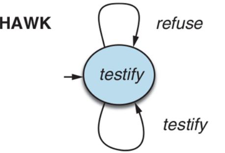
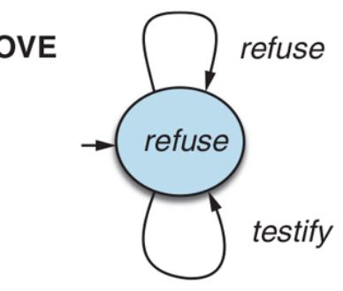
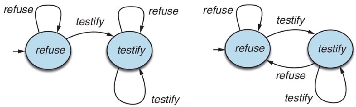
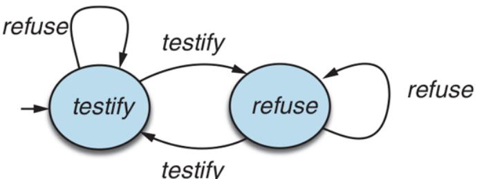
Some common, colorfully named finite-state machine strategies for the infinitely repeated prisoner’s dilemma.

Tit-for-Tat

The HAWK and DOVE strategies are simpler: HAWK simply plays testify on every round, while DOVE simply plays refuse on every round. The GRIM strategy is somewhat similar to TIT-FOR-TAT, but with one important difference: if ever its counterpart plays testify, then it essentially turns into HAWK: it plays testify forever. While TIT-FOR-TAT is forgiving, in the sense that it will respond to a subsequent refuse by reciprocating the same, with GRIM there is no way back. Just playing testify once will result in punishment (playing testify) that goes on forever. (Can you see what TIT-FOR-TAT does?)

The next issue with infinitely repeated games is how to measure the utility of an infinite sequence of payoffs. Here, we will focus on the limit of means approach—essentially, this means taking the average of utilities received over the infinite sequence. With this approach, given an infinite sequence of payoffs we define the utility of the sequence to the corresponding player to be:

\[\lim\_{T \to \infty} \frac{1}{T} \sum\_{t=0}^{T} U\_t.\]

Limit of means

This value cannot be guaranteed to converge for arbitrary sequences of utilities, but it is guaranteed to do so for the utility sequences that are generated if we use FSM strategies. To see this, observe that if FSM strategies play against each other, then eventually, the FSMs will reenter a configuration that they were in previously, at which point they will start to repeat themselves. More precisely, any utility sequence generated by FSM strategies will consist of a finite (possibly empty) non-repeating sequence, followed by a nonempty finite sequence that repeats infinitely often. To compute the average utility received by a player over that infinite sequence, we simply have to compute the average over the finite repeating sequence.

In what follows, we will assume that players in an infinitely repeated game simply choose a finite state machine to play the game on their behalf. We don’t impose any constraints on these machines: they can be as big and elaborate as players want. When all players have chosen a finite state machine to play on their behalf, then we can compute the payoffs for each player using the limit of means approach as described above. In this way, an infinitely

repeated game reduces to a normal form game, albeit one with infinitely many possible strategies for each player.

Let’s see what happens when we play the infinitely repeated prisoner’s dilemma using some strategies from Figure 18.3 . First, suppose Ali and Bo both pick DOVE.

It is not hard to see that this strategy pair does not form a Nash equilibrium: either player would have done better to alter their choice to HAWK. So, suppose Ali switches to HAWK:

This is the worst possible outcome for Bo; and this strategy pair is again not a Nash equilibrium. Bo would have done better by also choosing HAWK:

This strategy pair does form a Nash equilibrium, but not a very interesting one—it takes us more or less back to where we started in the one-shot version of the game, with both players testifying against each other. It illustrates a key property of infinitely repeated games: Nash equilibria of the stage game will be sustained as equilibria in an infinitely repeated version of the game.

However, our story is not over yet. Suppose that Bo switched to GRIM:

Here, Bo does no worse than playing HAWK: on the first round, Ali plays testify while Bo plays refuse, but this triggers Bo into testifying forever after: the loss of utility on the first round disappears in the limit. Overall, the two players get the same utility as if they had both played HAWK. But here is the thing: these strategies do not form a Nash equilibrium because this time, Ali has a beneficial deviation—to GRIM. If both players choose GRIM, then this is what happens:

The outcomes and payoffs are the same as if both players had chosen DOVE, but unlike that case, GRIM playing against GRIM forms a Nash equilibrium, and Ali and Bo are able to rationally achieve an outcome that is impossible in the one-shot version of the game.

To see that these strategies form a Nash equilibrium, suppose for the sake of contradiction that they do not. Then one player—assume without loss of generality that it is Ali—has a beneficial deviation, in the form of an FSM strategy that would yield a higher payoff than GRIM. Now, at some point this strategy would have to do something different from GRIM otherwise it would obtain the same utility. So, at some point it must play testify. But then Bo’s GRIM strategy would flip to punishment mode, by permanently testifying in response. At that point, Ali would be doomed to receive a payoff of no more than worse than the she would have received by choosing GRIM. Thus, both players choosing GRIM forms a Nash equilibrium in the infinitely repeated prisoner’s dilemma, giving a rationally sustained outcome that is impossible in the one-shot version of the game.

This is an instance of a general class of results called the Nash folk theorems, which characterize the outcomes that can be sustained by Nash equilibria in infinitely repeated games. Let’s say a player’s security value is the best payoff that the player could guarantee to obtain. Then the general form of the Nash folk theorems is roughly that every outcome in which every player receives at least their security value can be sustained as a Nash equilibrium in an infinitely repeated game. GRIM strategies are the key to the folk theorems: the mutual threat of punishment if any agent fails to play their part in the desired outcome keeps players in line. But it works as a deterrent only if the other player believes you have adopted this strategy or at least that you might have adopted it.

Nash folk theorems

We can also get different solutions by changing the agents, rather than changing the rules of engagement. Suppose the agents are finite state machines with states and they are playing a game with total steps. The agents are thus incapable of representing the number of remaining steps, and must treat it as an unknown. Therefore, they cannot do the backward induction, and are free to arrive at the more favorable (refuse, refuse) equilibrium in the iterated Prisoner’s Dilemma. In this case, ignorance is bliss—or rather, having your opponent believe that you are ignorant is bliss. Your success in these repeated games depends to a significant extent on the other player’s perception of you as a bully or a simpleton, and not on your actual characteristics.

18.2.4 Sequential games: The extensive form

In the general case, a game consists of a sequence of turns that need not be all the same. Such games are best represented by a game tree, which game theorists call the extensive form. The tree includes all the same information we saw in Section 5.1 : an initial state a function PLAYER that tells which player has the move, a function ACTIONS enumerating the possible actions, a function RESULT that defines the transition to a new state, and a partial function UTILITY which is defined only on terminal states, to give the payoff for each player. Stochastic games can be captured by introducing a distinguished player, Chance, that can take random actions. Chance’s “strategy” is part of the definition of the game, specified as a probability distribution over actions (the other players get to choose their own strategy). To represent games with nondeterministic actions, such as billiards, we break the action into two pieces: the player’s action itself has a deterministic result, and then Chance has a turn to react to the action in its own capricious way.

Extensive form

For the moment, we will make one simplifying assumption: we assume players have perfect information. Roughly, perfect information means that, when the game calls upon them to

make a decision, they know precisely where they are in the game tree: they have no uncertainty about what has happened previously in the game. This is, of course, the situation in games like chess or Go, but not in games like poker or Kriegspiel. In the following section, we will show how the extensive form can be used to capture imperfect information in games, but for the moment, we will assume perfect information.

Perfect information

A strategy in an extensive-form game of perfect information is a function for a player that for every one of its decision states dictates which action in ACTIONS the player should choose to execute. When each player has selected a strategy, then the resulting strategy profile will trace a path in the game tree from the initial state to a terminal state, and the UTILITY function defines the utilities that each player will then receive.

Given this setup, we can directly apply the apparatus of Nash equilibria that we introduced above to analyze extensive-form games. To compute Nash equilibria, we can use a straightforward generalization of the minimax search technique that we saw in Chapter 5 . In the literature on extensive-form games, the technique is called backward induction—we already saw backward induction informally used to analyze the finitely repeated prisoner’s dilemma. Backward induction uses dynamic programming, working backwards from terminal states back to the initial state, progressively labeling each state with a payoff profile (an assignment of payoffs to players) that would be obtained if the game was played optimally from that point on.

In more detail, for each nonterminal state if all the children of have been labeled with a payoff profile, then label with a payoff profile from the child state that maximizes the payoff of the player making the decision at state (If there is a tie, then choose arbitrarily; if we have chance nodes, then compute expected utility.) The backward induction algorithm is guaranteed to terminate, and moreover runs in time polynomial in the size of the game tree.

As the algorithm does its work, it traces out strategies for each player. As it turns out, these strategies are Nash equilibrium strategies, and the payoff profile labeling the initial state is a payoff profile that would be obtained by playing Nash equilibrium strategies. Thus, Nash equilibrium strategies for extensive-form games can be computed in polynomial time using backward induction; and since the algorithm is guaranteed to label the initial state with a payoff profile, it follows that every extensive-form game has at least one Nash equilibrium in pure strategies.

These are attractive results, but there are several caveats. Game trees very quickly get very large, so polynomial running time should be understood in that context. But more problematically, Nash equilibrium itself has some limitations when it is applied to extensiveform games. Consider the game in Figure 18.4 . Player 1 has two moves available: above or below If she moves below, then both players receive a payoff of 0 (regardless of the move selected by player 2). If she moves above, then player 2 is presented with a choice of moving up or down if she moves down, then both players receive a payoff of 0, while if she moves up, then they both receive 1.

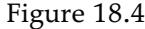
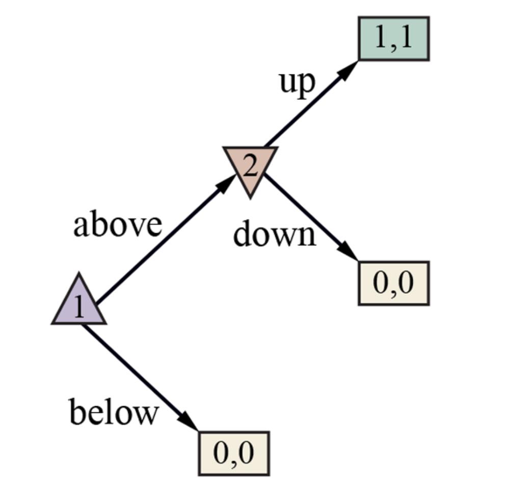
Backward induction immediately tells us that (above, up) is a Nash equilibrium, resulting in both players receiving a payoff of 1. However, (below, down) is also a Nash equilibrium, which would result in both players receiving a payoff of 0. Player 2 is threatening player 1, by indicating that if called upon to make a decision she will choose down, resulting in a payoff of 0 for player 1; in this case, player 1 has no better alternative than choosing below. The problem is that player 2’s threat (to play down) is not a credible threat, because if player 2 is actually called upon to make the choice, then she will choose up.

Credible threat

A refinement of Nash equilibrium called subgame perfect Nash equilibrium deals with this problem. To define it, we need the idea of a subgame. Every decision state in a game tree (including the initial state) defines a subgame—the game in Figure 18.4 therefore contains two subgames, one rooted at player 1’s decision state, one rooted at player 2’s decision state. A profile of strategies then forms a subgame perfect Nash equilibrium in a game if it is a Nash equilibrium in every subgame of Applying this definition to the game of Figure 18.4 , we find that (above, up) is subgame perfect, but (below, down) is not, because choosing down is not a Nash equilibrium of the subgame rooted at player 2’s decision state.

Subgame perfect

Nash equilibrium

Subgame

Although we needed some new terminology to define subgame perfect Nash equilibrium, we don’t need any new algorithms. The strategies computed through backward induction will be subgame perfect Nash equilibria, and it follows that every extensive-form game of perfect information has a subgame perfect Nash equilibrium, which can be computed in time polynomial in the size of the game tree.

Chance and simultaneous moves

To represent stochastic games, such as backgammon, in extensive form, we add a player called Chance, whose choices are determined by a probability distribution.

To represent simultaneous moves, as in the prisoner’s dilemma or two-finger Morra, we impose an arbitrary order on the players, but we have the option of asserting that the earlier player’s actions are not observable to the subsequent players: e.g., Ali must choose refuse or testify first, then Bo chooses, but Bo does not know what choice Ali made at that time (we can also represent the fact that the move is revealed later). However, we assume the players always remember all their own previous actions; this assumption is called perfect recall.

Capturing imperfect information

A key feature of extensive form that sets it apart from the game trees that we saw in Chapter 5 is that it can capture partial observability. Game theorists use the term imperfect information to describe situations where players are uncertain about the actual state of the game. Unfortunately, backward induction does not work with games of imperfect information, and in general, they are considerably more complex to solve than games of perfect information.

Imperfect information

We saw in Section 5.6 that a player in a partially observable game such as Kriegspiel can create a game tree over the space of belief states. With that tree, we saw that in some cases a player can find a sequence of moves (a strategy) that leads to a forced checkmate regardless of what actual state we started in, and regardless of what strategy the opponent uses. However, the techniques of Chapter 5 could not tell a player what to do when there is no guaranteed checkmate. If the player’s best strategy depends on the opponent’s strategy and vice versa, then minimax (or alpha–beta) by itself cannot find a solution. The extensive form does allow us to find solutions because it represents the belief states (game theorists call them information sets) of all players at once. From that representation we can find equilibrium solutions, just as we did with normal-form games.

Information set

As a simple example of a sequential game, place two agents in the world of Figure 17.1 and have them move simultaneously until one agent reaches an exit square and gets the payoff for that square. If we specify that no movement occurs when the two agents try to move into the same square simultaneously (a common problem at many traffic intersections), then certain pure strategies can get stuck forever. Thus, agents need a mixed strategy to perform well in this game: randomly choose between moving ahead and staying put. This is exactly what is done to resolve packet collisions in Ethernet networks.

Next we’ll consider a very simple variant of poker. The deck has only four cards, two aces and two kings. One card is dealt to each player. The first player then has the option to raise the stakes of the game from 1 point to 2, or to check. If player 1 checks, the game is over. If player 1 raises, then player 2 has the option to call, accepting that the game is worth 2 points, or fold, conceding the 1 point. If the game does not end with a fold, then the payoff depends on the cards: it is zero for both players if they have the same card; otherwise the player with the king pays the stakes to the player with the ace.

The extensive-form tree for this game is shown in Figure 18.5 . Player 0 is Chance; players 1 and 2 are depicted by triangles. Each action is depicted as an arrow with a label, corresponding to a raise, check, call, or fold, or, for Chance, the four possible deals (“AK” means that player 1 gets an ace and player 2 a king). Terminal states are rectangles labeled by their payoff to player 1 and player 2. Information sets are shown as labeled dashed boxes; for example, is the information set where it is player 1’s turn, and he knows he has an ace (but does not know what player 2 has). In information set it is player 2’s turn and she knows that she has an ace and that player 1 has raised, but does not know what

card player 1 has. (Due to the limits of two-dimensional paper, this information set is shown as two boxes rather than one.)

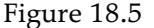
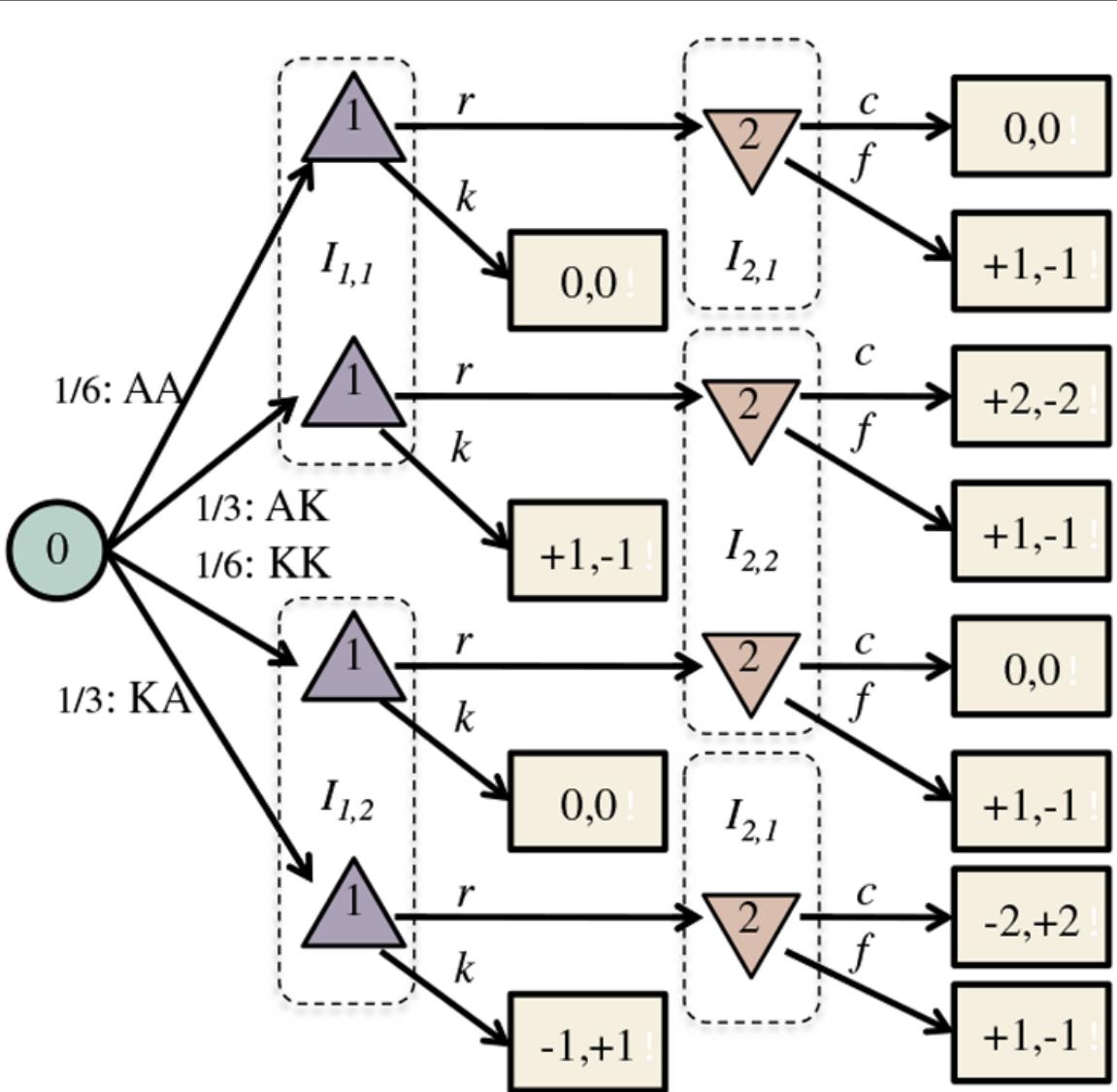
Extensive form of a simplified version of poker with two players and only four cards. The moves are r (raise), f (fold), c (call), and k (check).

One way to solve an extensive game is to convert it to a normal-form game. Recall that the normal form is a matrix, each row of which is labeled with a pure strategy for player 1, and each column by a pure strategy for player 2. In an extensive game a pure strategy for player i corresponds to an action for each information set involving that player. So in Figure 18.5 , one pure strategy for player 1 is “raise when in (that is, when I have an ace), and check

when in (when I have a king).” In the payoff matrix below, this strategy is called . Similarly, strategy for player 2 means “call when I have an ace and fold when I have a king.” Since this is a zero-sum game, the matrix below gives only the payoff for player 1; player 2 always has the opposite payoff:

	2:cc	2:cf	2:ff	2:fc
l:rr	0	-1/6	1	716
1:kr	-1/3	-1/6	5/6	2/3
l:rk	1/3	0	116	1/2
l:kk	0	0	0	0

This game is so simple that it has two pure-strategy equilibria, shown in bold: for player 2 and or for player 1. But in general we can solve extensive games by converting to normal form and then finding a solution (usually a mixed strategy) using standard linear programming methods. That works in theory. But if a player has information sets and actions per set, then that player will have pure strategies. In other words, the size of the normal-form matrix is exponential in the number of information sets, so in practice the approach works only for tiny game trees—a dozen states or so. A game like two-player Texas hold ’em poker has about states, making this approach completely infeasible.

What are the alternatives? In Chapter 5 we saw how alpha–beta search could handle games of perfect information with huge game trees by generating the tree incrementally, by pruning some branches, and by heuristically evaluating nonterminal nodes. But that approach does not work well for games with imperfect information, for two reasons: first, it is harder to prune, because we need to consider mixed strategies that combine multiple branches, not a pure strategy that always chooses the best branch. Second, it is harder to heuristically evaluate a nonterminal node, because we are dealing with information sets, not individual states.

Koller et al., (1996) came to the rescue with an alternative representation of extensive games, called the sequence form, that is only linear in the size of the tree, rather than exponential. Rather than represent strategies, it represents paths through the tree; the number of paths is equal to the number of terminal nodes. Standard linear programming methods can again be applied to this representation. The resulting system can solve poker variants with 25,000 states in a minute or two. This is an exponential speedup over the

normal-form approach, but still falls far short of handling, say, two-player Texas hold ’em, with states.

Sequence form

If we can’t handle states, perhaps we can simplify the problem by changing the game to a simpler form. For example, if I hold an ace and am considering the possibility that the next card will give me a pair of aces, then I don’t care about the suit of the next card; under the rules of poker any suit will do equally well. This suggests forming an abstraction of the game, one in which suits are ignored. The resulting game tree will be smaller by a factor of Suppose I can solve this smaller game; how will the solution to that game relate to the original game? If no player is considering going for a flush (the only hand where the suits matter), then the solution for the abstraction will also be a solution for the original game. However, if any player is contemplating a flush, then the abstraction will be only an approximate solution (but it is possible to compute bounds on the error).

There are many opportunities for abstraction. For example, at the point in a game where each player has two cards, if I hold a pair of queens, then the other players’ hands could be abstracted into three classes: better (only a pair of kings or a pair of aces), same (pair of queens) or worse (everything else). However, this abstraction might be too coarse. A better abstraction would divide worse into, say, medium pair (nines through jacks), low pair, and no pair. These examples are abstractions of states; it is also possible to abstract actions. For example, instead of having a bet action for each integer from 1 to 1000, we could restrict the bets to and Or we could cut out one of the rounds of betting altogether. We can also abstract over chance nodes, by considering only a subset of the possible deals. This is equivalent to the rollout technique used in Go programs. Putting all these abstractions together, we can reduce the states of poker to states, a size that can be solved with current techniques.

We saw in Chapter 5 how poker programs such as Libratus and DeepStack were able to defeat champion human players at heads up (two-player) Texas hold ’em poker. More recently, the program Pluribus was able to defeat human champions at six-player poker in two formats: five copies of the program at the table with one human, and one copy of the program with five humans. There is a huge leap in complexity here. With one opponent, there are possibilities for the opponent’s hidden cards. But with five opponents there are billion possibilities. Pluribus develops a baseline strategy entirely from self-play, then modifies the strategy during actual game play to react to a specific situation. Pluribus uses a combination of techniques, including Monte Carlo tree search, depth-limited search, and abstraction.

The extensive form is a versatile representation: it can handle partially observable, multiagent, stochastic, sequential, real-time environments—most of the hard cases from the list of environment properties on page 43. However, there are two limitations to the extensive form in particular and game theory in general. First, it does not deal well with continuous states and actions (although there have been some extensions to the continuous case; for example, the theory of Cournot competition uses game theory to solve problems where two companies choose prices for their products from a continuous space). Second, game theory assumes the game is known. Parts of the game may be specified as unobservable to some of the players, but it must be known what parts are unobservable. In cases in which the players learn the unknown structure of the game over time, the model begins to break down. Let’s examine each source of uncertainty, and whether each can be represented in game theory.

Cournot competition

Actions: There is no easy way to represent a game where the players have to discover what actions are available. Consider the game between computer virus writers and security experts. Part of the problem is anticipating what action the virus writers will try next.

Strategies: Game theory is very good at representing the idea that the other players’ strategies are initially unknown—as long as we assume all agents are rational. The theory does not say what to do when the other players are less than fully rational. The notion of a Bayes–Nash equilibrium partially addresses this point: it is an equilibrium with respect to a player’s prior probability distribution over the other players’ strategies—in other words, it expresses a player’s beliefs about the other players’ likely strategies.

Bayes–Nash equilibrium

Chance: If a game depends on the roll of a die, it is easy enough to model a chance node with uniform distribution over the outcomes. But what if it is possible that the die is unfair? We can represent that with another chance node, higher up in the tree, with two branches for “die is fair” and “die is unfair,” such that the corresponding nodes in each branch are in the same information set (that is, the players don’t know if the die is fair or not). And what if we suspect the other opponent does know? Then we add another chance node, with one branch representing the case where the opponent does know, and one where the opponent doesn’t.

Utilities: What if we don’t know our opponent’s utilities? Again, that can be modeled with a chance node, such that the other agent knows its own utilities in each branch, but we don’t. But what if we don’t know our own utilities? For example, how do I know if it is rational to order the chef’s salad if I don’t know how much I will like it? We can model that with yet another chance node specifying an unobservable “intrinsic quality” of the salad.

Thus, we see that game theory is good at representing most sources of uncertainty—but at the cost of doubling the size of the tree every time we add another node; a habit that quickly leads to intractably large trees. Because of these and other problems, game theory has been used primarily to analyze environments that are at equilibrium, rather than to control agents within an environment.

18.2.5 Uncertain payoffs and assistance games

In Chapter 1 (page 4), we noted the importance of designing AI systems that can operate under uncertainty about the true human objective. Chapter 16 (page 553) introduced a simple model for uncertainty about one’s own preferences, using the example of durianflavored ice cream. By the simple device of adding a new latent variable to the model to represent the unknown preferences, together with an appropriate sensor model (e.g.,

observing the taste of a small sample of the ice cream), uncertain preferences can be handled in a natural way.

Chapter 16 also studied the off-switch problem: we showed that a robot with uncertainty about human preferences will defer to the human and allow itself to be switched off. In that problem, Robbie the robot is uncertain about Harriet the human’s preferences, but we model Harriet’s decision (whether or not to switch Robbie off) as a simple, deterministic consequence of her own preferences for the action that Robbie proposes. Here, we generalize this idea into a full two-person game called an assistance game, in which both Harriet and Robbie are players. We assume that Harriet observes her own preferences and acts in accordance with them, while Robbie has a prior probability over Harriet’s preferences. The payoff is defined by and is identical for both players: both Harriet and Robbie are maximizing Harriet’s payoff. In this way, the assistance game provides a formal model of the idea of provably beneficial AI introduced in Chapter 1 .

In addition to the deferential behavior exhibited by Robbie in the off-switch problem which is a restricted kind of assistance game—other behaviors that emerge as equilibrium strategies in general assistance games include actions on Harriet’s part that we would describe as teaching, rewarding, commanding, correcting, demonstrating, or explaining, as well as actions on Robbie’s part that we would describe as asking permission, learning from demonstrations, preference elicitation, and so on. The key point is that these behaviors need not be scripted: by solving the game, Harriet and Robbie work out for themselves how to convey preference information from Harriet to Robbie, so that Robbie can be more useful to Harriet. We need not stipulate in advance that Harriet is to “give rewards” or that Robbie is to “follow instructions,” although these may be reasonable interpretations of how they end up behaving.

To illustrate assistance games, we’ll use the paperclip game. It’s a very simple game in which Harriet the human has an incentive to “signal” to Robbie the robot some information about her preferences. Robbie is able to interpret that signal because he can solve the game and therefore he can understand what would have to be true about Harriet’s preferences in order for her to signal in that way.

Paperclip game

The steps of the game are depicted in Figure 18.6 . It involves making paperclips and staples. Harriet’s preferences are expressed by a payoff function that depends on the number of paperclips and the number of staples produced, with a certain “exchange rate” between the two. Harriet’s preference parameter denotes the relative value (in dollars) of a paperclip; for example, she might value paperclips at dollars, which means staples are worth dollars. So, if paperclips and staples are produced, Harriet’s payoff will be dollars in all. Robbie’s prior is In the game itself, Harriet goes first, and can choose to make two paperclips, two staples, or one of each. Then Robbie can choose to make 90 paperclips, 90 staples, or 50 of each.

Figure 18.6

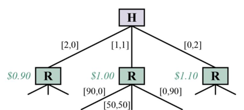
The paperclip game. Each branch is labeled denoting the number of paperclips and staples manufactured on that branch. Harriet the human can choose to make two paperclips, two staples, or one of each. (The values in green italics are the values for Harriet if the game ended there, assuming ) Robbie the robot then has a choice to make 90 paperclips, 90 staples, or 50 of each.

Notice that if she were doing this by herself, Harriet would just make two staples, with a value of $1.10. (See the annotations at the first level of the tree in Figure 18.6 .) But Robbie is watching, and he learns from her choice. What exactly does he learn? Well, that depends on how Harriet makes her choice. How does Harriet make her choice? That depends on how Robbie is going to interpret it. We can resolve this circularity by finding a Nash equilibrium. In this case, it is unique and can be found by applying myopic best response: pick any strategy for Harriet; pick the best strategy for Robbie, given Harriet’s strategy; pick the best strategy for Harriet, given Robbie’s strategy; and so on. The process unfolds as follows:

• 1. Start with the greedy strategy for Harriet: make two paperclips if she prefers paperclips; make one of each if she is indifferent; make two staples if she prefers staples.
• 2. There are three possibilities Robbie has to consider, given this strategy for Harriet:
  • a. If Robbie sees Harriet make two paperclips, he infers that she prefers paperclips, so he now believes the value of a paperclip is uniformly distributed between 0.5 and 1.0, with an average of 0.75. In that case, his best plan is to make 90 paperclips with an expected value of $67.50 for Harriet.
  • b. If Robbie sees Harriet make one of each, he infers that she values paperclips and staples at 0.50, so the best choice is to make 50 of each.
  • c. If Robbie sees Harriet make two staples, then by the same argument as in (a), he should make 90 staples.
• 3. Given this strategy for Robbie, Harriet’s best strategy is now somewhat different from the greedy strategy in step 1. If Robbie is going to respond to her making one of each by making 50 of each, then she is better off making one of each not just if she is exactly indifferent, but if she is anywhere close to indifferent. In fact, the optimal policy is now to make one of each if she values paperclips anywhere between about 0.446 and 0.554.
• 4. Given this new strategy for Harriet, Robbie’s strategy remains unchanged. For example, if she chooses one of each, he infers that the value of a paperclip is uniformly distributed between 0.446 and 0.554, with an average of 0.50, so the best choice is to make 50 of each. Because Robbie’s strategy is the same as in step 2, Harriet’s best response will be the same as in step 3, and we have found the equilibrium.

With her strategy, Harriet is, in effect, teaching Robbie about her preferences using a simple code–—a language, if you like–—that emerges from the equilibrium analysis. Note also that Robbie never learns Harriet’s preferences exactly, but he learns enough to act optimally on her behalf–—i.e., he acts just as he would if he did know her preferences exactly. He is provably beneficial to Harriet under the assumptions stated, and under the assumption that Harriet is playing the game correctly.

Myopic best response works for this example and others like it, but not for more complex cases. It is possible to prove that provided there are no ties that cause coordination

problems, finding an optimal strategy profile for an assistance game is reducible to solving a POMDP whose state space is the underlying state space of the game plus the human preference parameters POMDPs in general are very hard to solve (Section 17.5 ), but the POMDPs that represent assistance games have additional structure that enables more efficient algorithms.

Assistance games can be generalized to allow for multiple human participants, multiple robots, imperfectly rational humans, humans who don’t know their own preferences, and so on. By providing a factored or structured action space, as opposed to the simple atomic actions in the paperclip game, the opportunities for communication can be greatly enhanced. Few of these variations have been explored so far, but we expect the key property of assistance games to remain true: the more intelligent the robot, the better the outcome for the human.

18.3 Cooperative Game Theory

Recall that cooperative games capture decision making scenarios in which agents can form binding agreements with one another to cooperate. They can then benefit from receiving extra value compared to what they would get by acting alone.

We start by introducing a model for a class of cooperative games. Formally, these games are called “cooperative games with transferable utility in characteristic function form.” The idea of the model is that when a group of agents cooperate, the group as a whole obtains some utility value, which can then be split among the group members. The model does not say what actions the agents will take, nor does the game structure itself specify how the value obtained will be split up (that will come later).

Formally, we use the formula to say that a cooperative game, is defined by a set of players and a characteristic function, which for every subset of players gives the value that the group of players could obtain, should they choose to work together.

Characteristic function

Typically, we assume that the empty set of players achieves nothing ( ), and that the function is nonnegative ( for all ). In some games we make the further assumption that players achieve nothing by working alone: for all

18.3.1 Coalition structures and outcomes

It is conventional to refer to a subset of players as a coalition. In everyday use the term “coalition” implies a collection of people with some common cause (such as the Coalition to Stop Gun Violence), but we will refer to any subset of players as a coalition. The set of all players is known as the grand coalition.

Coalition

Grand coalition

In our model, every player must choose to join exactly one coalition (which could be a coalition of just the single player alone). Thus, the coalitions form a partition of the set of players. We call the partition a coalition structure. Formally, a coalition structure over a set of players is a set of coalitions such that:

\[\begin{aligned} C\_i &\neq \{\} \\ C\_i &\subseteq N \\ C\_i \cap C\_j &= \{\} \text{ for all } i \neq j \in N \\ C\_1 \cup \ldots \cup C\_k &= N. \end{aligned}\]

Coalition structure

For example, if we have then there are seven possible coalitions:

\[\{1\}, \{2\}, \{3\}, \{1,2\}, \{2,3\}, \{3,1\}, \text{ and } \{1,2,3\}\]

and five possible coalition structures:

We use the notation to denote the set of all coalition structures over player set and to denote the coalition that player belongs to.

The outcome of a game is defined by the choices the players make, in deciding which coalitions to form, and in choosing how to divide up the value that each coalition receives. Formally, given a cooperative game defined by the outcome is a pair consisting of a coalition structure and a payoff vector where is the value that goes to player The payoff must satisfy the constraint that each coalition splits up all of its value among its members:

\[\sum\_{i \in C} x\_i = \nu(C) \qquad \text{for all } C \in CS\]

Payoff vector

For example, given the game where and a possible outcome is:

\[(\{\{1\}, \{2,3\}\}, (4,5,5)).\]

That is, player 1 stays alone and accepts a value of 4, while players 2 and 3 team up to receive a value of 10, which they choose to split evenly.

Some cooperative games have the feature that when two coalitions merge together, they do no worse than if they had stayed apart. This property is called superadditivity. Formally, a game is superadditive if its characteristic function satisfies the following condition:

\[ \nu(C \cup D) \ge \nu(C) + \nu(D) \qquad \text{for all } C, D \subseteq N \]

Superadditivity

If a game is superadditive, then the grand coalition receives a value that is at least as high as or higher than the total received by any other coalition structure. However, as we will see shortly, superadditive games do not always end up with a grand coalition, for much the

same reason that the players do not always arrive at a collectively desirable Pareto-optimal outcome in the prisoner’s dilemma.

18.3.2 Strategy in cooperative games

The basic assumption in cooperative game theory is that players will make strategic decisions about who they will cooperate with. Intuitively, players will not desire to work with unproductive players—they will naturally seek out players that collectively yield a high coalitional value. But these sought-after players will be doing their own strategic reasoning. Before we can describe this reasoning, we need some further definitions.

An imputation for a cooperative game is a payoff vector that satisfies the following two conditions:

\[\begin{aligned} \sum\_{i=1}^{n} x\_i &= v(N) \\ x\_i &\ge v\left(\{i\}\right) \text{ for all } i \in N \end{aligned}\]

Imputation

The first condition says that an imputation must distribute the total value of the grand coalition; the second condition, known as individual rationality, says that each player is at least as well off as if it had worked alone.

Individual rationality

Given an imputation and a coalition we define to be the sum —the total amount disbursed to by the imputation

Next, we define the core of a game as the set of all imputations that satisfy the condition for every possible coalition Thus, if an imputation is not in the core, then there exists some coalition such that The players in would refuse to join the grand coalition because they would be better off sticking with

Core

The core of a game therefore consists of all the possible payoff vectors that no coalition could object to on the grounds that they could do better by not joining the grand coalition. Thus, if the core is empty, then the grand coalition cannot form, because no matter how the grand coalition divided its payoff, some smaller coalition would refuse to join. The main computational questions around the core relate to whether or not it is empty, and whether a particular payoff distribution is in the core.

The definition of the core naturally leads to a system of linear inequalities, as follows (the unknowns are variables and the values are constants):

\[\begin{array}{rcl} x\_i & \ge & \nu(\{i\}) \quad \text{for all } i \in N\\ \sum\_{i \in N} x\_i & = & \nu(N) \\ \sum\_{i \in C} x\_i & \ge & \nu(C) \quad \text{for all } C \subseteq N \end{array}\]

Any solution to these inequalities will define an imputation in the core. We can formulate the inequalities as a linear program by using a dummy objective function (for example, maximizing ), which will allow us to compute imputations in time polynomial in the number of inequalities. The difficulty is that this gives an exponential number of inequalities (one for each of the possible coalitions). Thus, this approach yields an algorithm for checking non-emptiness of the core that runs in exponential time. Whether we can do better than this depends on the game being studied: for many classes of cooperative game, the problem of checking non-emptiness of the core is co-NP-complete. We give an example below.

Before proceeding, let’s see an example of a superadditive game with an empty core. The game has three players and has a characteristic function defined as follows:

\[\nu(C) = \begin{cases} 1 & \text{if } |C| \ge 2 \\ 0 & \text{otherwise} \end{cases}\]

Now consider any imputation for this game. Since it must be the case that at least one player has and the other two get a total payoff less than 1. Those two could benefit by forming a coalition without player and sharing the value 1 among themselves. But since this holds for all imputations, the core must be empty.

The core formalizes the idea of the grand coalition being stable, in the sense that no coalition can profitably defect from it. However, the core may contain imputations that are unreasonable, in the sense that one or more players might feel they were unfair. Suppose and we have a characteristic function defined as follows:

\[\begin{aligned} \nu(\{1\}) &= \nu(\{2\}) = 5 \\ \nu(\{1, 2\}) &= 20. \end{aligned}\]

Here, cooperation yields a surplus of 10 over what players could obtain working in isolation, and so intuitively, cooperation will make sense in this scenario. Now, it is easy to see that the imputation (6,14) is in the core of this game: neither player can deviate to obtain a higher utility. But from the point of view of player 1, this might appear unreasonable, because it gives 9/10 of the surplus to player 2. Thus, the notion of the core tells us when a grand coalition can form, but it does not tell us how to distribute the payoff.

The Shapley value is an elegant proposal for how to divide the value among the players, given that the grand coalition formed. Formulated by Nobel laureate Lloyd Shapley in the early 1950s, the Shapley value is intended to be a fair distribution scheme.

Shapley value

What does fair mean? It would be unfair to distribute based on the eye color of players, or their gender, or skin color. Students often suggest that the value should be divided equally, which seems like it might be fair, until we consider that this would give the same reward to players that contribute a lot and players that contribute nothing. Shapley’s insight

was to suggest that the only fair way to divide the value was to do so according to how much each player contributed to creating the value

First we need to define the notion of a player’s marginal contribution. The marginal contribution that a player makes to a coalition is the value that would add (or remove), should join the coalition Formally, the marginal contribution that player makes to is denoted by

\[mc\_i(C) = \nu(C \cup \{i\}) - \nu(C).\]

Marginal contribution

Now, a first attempt to define a payoff division scheme in line with Shapley’s suggestion that players should be rewarded according to their contribution would be to pay each player the value that they would add to the coalition containing all other players:

\[mc\_i(N - \{i\}).\]

The problem is that this implicitly assumes that player is the last player to enter the coalition. So, Shapley suggested, we need to consider all possible ways that the grand coalition could form, that is, all possible orderings of the players and consider the value that adds to the preceding players in the ordering. Then, a player should be rewarded by being paid the average marginal contribution that player makes, over all possible orderings of the players, to the set of players preceding in the ordering.

We let denote all possible permutations (e.g., orderings) of the players and denote members of by etc. Where and we denote by the set of players that precede in the ordering Then the Shapley value for a game is the imputation defined as follows:

(18.1)

\[\phi\_i(G) = \frac{1}{n!} \sum\_{p \in P} mc\_i(p\_i).\]

This should convince you that the Shapley value is a reasonable proposal. But the remarkable fact is that it is the unique solution to a set of axioms that characterizes a “fair” payoff distribution scheme. We’ll need some more definitions before defining the axioms.

We define a dummy player as a player that never adds any value to a coalition—that is, for all We will say that two players and are symmetric players if they always make identical contributions to coalitions—that is, for all Finally, where and are games with the same set of players, the game is the game with the same player set, and a characteristic function defined by

Dummy player

Symmetric players

Given these definitions, we can define the fairness axioms satisfied by the Shapley value:

• EFFICIENCY: (All the value should be distributed.)
• DUMMY PLAYER: If is a dummy player in then (Players who never contribute anything should never receive anything.)
• SYMMETRY: If and are symmetric in then (Players who make identical contributions should receive identical payoffs.)
• ADDITIVITY: The value is additive over games: For all games and and for all players we have

The additivity axiom is admittedly rather technical. If we accept it as a requirement, however, we can establish the following key property: the Shapley value is the only way to distribute coalitional value so as to satisfy these fairness axioms.

18.3.3 Computation in cooperative games

From a theoretical point of view, we now have a satisfactory solution. But from a computational point of view, we need to know how to compactly represent cooperative games, and how to efficiently compute solution concepts such as the core and the Shapley value.

The obvious representation for a characteristic function would be a table listing the value for all coalitions. This is infeasible for large A number of approaches to compactly representing cooperative games have been developed, which can be distinguished by whether or not they are complete. A complete representation scheme is one that is capable of representing any cooperative game. The drawback with complete representation schemes is that there will always be some games that cannot be represented compactly. An alternative is to use a representation scheme that is guaranteed to be compact, but which is not complete.

Marginal contribution nets

We now describe one representation scheme, called marginal contribution nets (MC-nets). We will use a slightly simplified version to facilitate presentation, and the simplification makes it incomplete—the full version of MC-nets is a complete representation.

Marginal contribution net

The idea behind marginal contribution nets is to represent the characteristic function of a game as a set of coalition-value rules, of the form: where is a coalition and is a number. To compute the value of a coalition we simply sum the values of all rules such that Thus, given a set of rules the corresponding characteristic function is:

\[\nu(C) = \sum \{x\_i \mid (C\_i, x\_i) \in R \text{ and } C\_i \subseteq C\}.\]

Suppose we have a rule set containing the following three rules:

\[\{ (\{1,2\},5), \quad (\{2\},2), \quad (\{3\},4) \}.\]

Then, for example, we have:

• (because no rules apply),
• (third rule),
• (third rule),
• (second and third rules), and
• (first, second, and third rules).

With this representation we can compute the Shapley value in polynomial time. The key insight is that each rule can be understood as defining a game on its own, in which the players are symmetric. By appealing to Shapley’s axioms of additivity and symmetry, therefore, the Shapley value of player in the game associated with the rule set is then simply:

\[\phi\_i(R) = \sum\_{(C,x)\in R} \begin{cases} \frac{x}{|C|} & \text{if } i \in C\\ 0 & \text{otherwise.} \end{cases}\]

The version of marginal contribution nets that we have presented here is not a complete representation scheme: there are games whose characteristic function cannot be represented using rule sets of the form described above. A richer type of marginal contribution networks allows for rules of the form where is a propositional logic formula over the players a coalition satisfies the condition if it corresponds to a satisfying assignment for This scheme is a complete representation—in the worst case, we need a rule for every possible coalition. Moreover, the Shapley value can be computed in polynomial time with this scheme; the details are more involved than for the simple rules described above, although the basic principle is the same; see the notes at the end of the chapter for references.

Coalition structures for maximum social welfare

We obtain a different perspective on cooperative games if we assume that the agents share a common purpose. For example, if we think of the agents as being workers in a company, then the strategic considerations relating to coalition formation that are addressed by the core, for example, are not relevant. Instead, we might want to organize the workforce (the agents) into teams so as to maximize their overall productivity. More generally, the task is to find a coalition that maximizes the social welfare of the system, defined as the sum of the

values of the individual coalitions. We write the social welfare of a coalition structure as with the following definition:

\[sw(CS) = \sum\_{C \in CS} \nu(C).\]

Then a socially optimal coalition structure with respect to maximizes this quantity. Finding a socially optimal coalition structure is a very natural computational problem, which has been studied beyond the multiagent systems community: it is sometimes called the set partitioning problem. Unfortunately, the problem is NP-hard, because the number of possible coalition structures grows exponentially in the number of players.

Set partitioning problem

Finding the optimal coalition structure by naive exhaustive search is therefore infeasible in general. An influential approach to optimal coalition structure formation is based on the idea of searching a subspace of the coalition structure graph. The idea is best explained with reference to an example.

Coalition structure graph

Suppose we have a game with four agents, There are fifteen possible coalition structures for this set of agents. We can organize these into a coalition structure graph as shown in Figure 18.7 , where the nodes at level of the graph correspond to all the coalition structures with exactly coalitions. An upward edge in the graph represents the division of a coalition in the lower node into two separate coalitions in the upper node. For example, there is an edge from to because this latter coalition structure is obtained from the former by dividing the coalition into the coalitions and

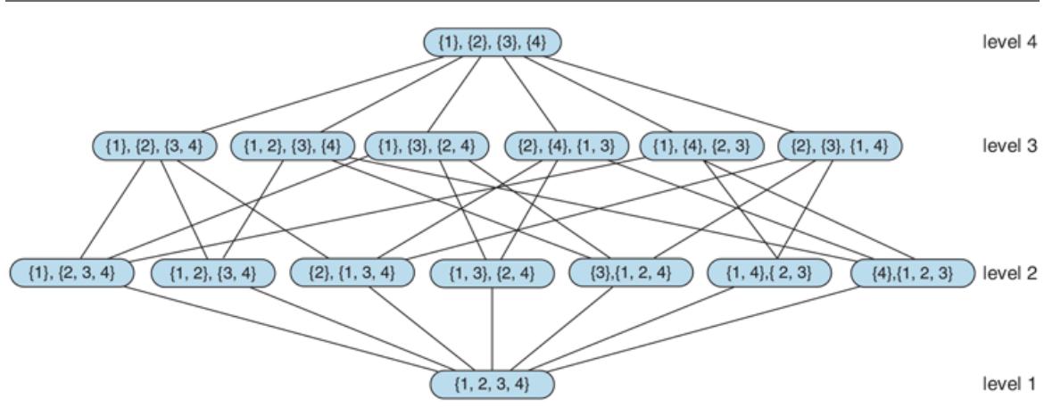
The coalition structure graph for Level 1 has coalition structures containing a single coalition; level 2 has coalition structures containing two coalitions, and so on.

The optimal coalition structure lies somewhere within the coalition structure graph, and so to find this, it seems we would have to evaluate every node in the graph. But consider the bottom two rows of the graph—levels 1 and 2. Every possible coalition (excluding the empty coalition) appears in these two levels. (Of course, not every possible coalition structure appears in these two levels.) Now, suppose we restrict our search for a possible coalition structure to just these two levels—we go no higher in the graph. Let be the best coalition structure that we find in these two levels, and let be the best coalition structure overall. Let be a coalition with the highest value of all possible coalitions:

\[C^\* \in \arg\max\_{C \subseteq N} \nu(C).\]

The value of the best coalition structure we find in the first two levels of the coalition structure graph must be at least as much as the value of the best possible coalition: This is because every possible coalition appears in at least one coalition structure in the first two levels of the graph. So assume the worst case, that is,

Compare the value of to Since is the highest possible value of any coalition structure, and there are agents ( in the case of Figure 18.7 ), then the highest possible value of would be In other words, in the worst possible case, the value of the best coalition structure we find in the first two levels of the graph would be the value of the best, where is the number of agents. Thus, although searching the first two levels of the graph does not guarantee to give us the optimal coalition structure, it does guarantee to give us one that is no worse that of the optimal. In practice it will often be much better than that.

18.4 Making Collective Decisions

We will now turn from agent design to mechanism design—the problem of designing the right game for a collection of agents to play. Formally, a mechanism consists of

• 1. A language for describing the set of allowable strategies that agents may adopt.
• 2. A distinguished agent, called the center, that collects reports of strategy choices from the agents in the game. (For example, the auctioneer is the center in an auction.)

Center

3. An outcome rule, known to all agents, that the center uses to determine the payoffs to each agent, given their strategy choices.

This section discusses some of the most important mechanisms.

18.4.1 Allocating tasks with the contract net

The contract net protocol is probably the oldest and most important multiagent problemsolving technique studied in AI. It is a high-level protocol for task sharing. As the name suggests, the contract net was inspired from the way that companies make use of contracts.

Contract net protocol

The overall contract net protocol has four main phases—see Figure 18.8 . The process starts with an agent identifying the need for cooperative action with respect to some task. The need might arise because the agent does not have the capability to carry out the task in

isolation, or because a cooperative solution might in some way be better (faster, more efficient, more accurate).

The contract net task allocation protocol.

The agent advertises the task to other agents in the net with a task announcement message, and then acts as the manager of that task for its duration. The task announcement message must include sufficient information for recipients to judge whether or not they are willing and able to bid for the task. The precise information included in a task announcement will depend on the application area. It might be some code that needs to be executed; or it might be a logical specification of a goal to be achieved. The task announcement might also

include other information that might be required by recipients, such as deadlines, quality-ofservice requirements, and so on.

Task announcement

Manager

When an agent receives a task announcement, it must evaluate it with respect to its own capabilities and preferences. In particular, each agent must determine, whether it has the capability to carry out the task, and second, whether or not it desires to do so. On this basis, it may then submit a bid for the task. A bid will typically indicate the capabilities of the bidder that are relevant to the advertised task, and any terms and conditions under which the task will be carried out.

Bid

In general, a manager may receive multiple bids in response to a single task announcement. Based on the information in the bids, the manager selects the most appropriate agent (or agents) to execute the task. Successful agents are notified through an award message, and become contractors for the task, taking responsibility for the task until it is completed.

The main computational tasks required to implement the contract net protocol can be summarized as follows:

TASK ANNOUNCEMENT PROCESSING. On receipt of a task announcement, an agent decides if it wishes to bid for the advertised task.

• BID PROCESSING. On receiving multiple bids, the manager must decide which agent to award the task to, and then award the task.
• AWARD PROCESSING. Successful bidders (contractors) must attempt to carry out the task, which may mean generating new subtasks, which are advertised via further task announcements.

Despite (or perhaps because of) its simplicity, the contract net is probably the most widely implemented and best-studied framework for cooperative problem solving. It is naturally applicable in many settings—a variation of it is enacted every time you request a car with Uber, for example.

18.4.2 Allocating scarce resources with auctions

One of the most important problems in multiagent systems is that of allocating scarce resources; but we may as well simply say “allocating resources,” since in practice most useful resources are scarce in some sense. The auction is the most important mechanism for allocating resources. The simplest setting for an auction is where there is a single resource and there are multiple possible bidders. Each bidder has a utility value for the item.

Auction

Bidder

In some cases, each bidder has a private value for the item. For example, a tacky sweater might be attractive to one bidder and valueless to another.

In other cases, such as auctioning drilling rights for an oil tract, the item has a common value—the tract will produce some amount of money, and all bidders value a dollar equally—but there is uncertainty as to what the actual value of is. Different bidders have different information, and hence different estimates of the item’s true value. In either case, bidders end up with their own Given each bidder gets a chance, at the appropriate

time or times in the auction, to make a bid The highest bid, wins the item, but the price paid need not be that’s part of the mechanism design.

The best-known auction mechanism is the ascending-bid auction, or English auction, in which the center starts by asking for a minimum (or reserve) bid If some bidder is willing to pay that amount, the center then asks for for some increment and continues up from there. The auction ends when nobody is willing to bid anymore; then the last bidder wins the item, paying the price bid. 3

3 The word “auction” comes from the Latin augeo, to increase.

Ascending-bid auction

English auction

How do we know if this is a good mechanism? One goal is to maximize expected revenue for the seller. Another goal is to maximize a notion of global utility. These goals overlap to some extent, because one aspect of maximizing global utility is to ensure that the winner of the auction is the agent who values the item the most (and thus is willing to pay the most). We say an auction is efficient if the goods go to the agent who values them most. The ascending-bid auction is usually both efficient and revenue maximizing, but if the reserve price is set too high, the bidder who values it most may not bid, and if the reserve is set too low, the seller may get less revenue.

Efficient

Collusion

Probably the most important things that an auction mechanism can do is encourage a sufficient number of bidders to enter the game and discourage them from engaging in collusion. Collusion is an unfair or illegal agreement by two or more bidders to manipulate prices. It can happen in secret backroom deals or tacitly, within the rules of the mechanism. For example, in 1999, Germany auctioned ten blocks of cellphone spectrum with a simultaneous auction (bids were taken on all ten blocks at the same time), using the rule that any bid must be a minimum of a 10% raise over the previous bid on a block. There were only two credible bidders, and the first, Mannesman, entered the bid of 20 million deutschmark on blocks 1-5 and 18.18 million on blocks 6-10. Why 18.18M? One of T-Mobile’s managers said they “interpreted Mannesman’s first bid as an offer.” Both parties could compute that a 10% raise on 18.18M is 19.99M; thus Mannesman’s bid was interpreted as saying “we can each get half the blocks for 20M; let’s not spoil it by bidding the prices up higher.” And in fact T-Mobile bid 20M on blocks 6-10 and that was the end of the bidding.

The German government got less than they expected, because the two competitors were able to use the bidding mechanism to come to a tacit agreement on how not to compete. From the government’s point of view, a better result could have been obtained by any of these changes to the mechanism: a higher reserve price; a sealed-bid first-price auction, so that the competitors could not communicate through their bids; or incentives to bring in a third bidder. Perhaps the 10% rule was an error in mechanism design, because it facilitated the precise signaling from Mannesman to T-Mobile.

In general, both the seller and the global utility function benefit if there are more bidders, although global utility can suffer if you count the cost of wasted time of bidders that have no chance of winning. One way to encourage more bidders is to make the mechanism easier for them. After all, if it requires too much research or computation on the part of the bidders, they may decide to take their money elsewhere.

So it is desirable that the bidders have a dominant strategy. Recall that “dominant” means that the strategy works against all other strategies, which in turn means that an agent can adopt it without regard for the other strategies. An agent with a dominant strategy can just bid, without wasting time contemplating other agents’ possible strategies. A mechanism by which agents have a dominant strategy is called a strategy-proof mechanism. If, as is usually the case, that strategy involves the bidders revealing their true value, then it is called a truth-revealing, or truthful, auction; the term incentive compatible is also used. The revelation principle states that any mechanism can be transformed into an equivalent truthrevealing mechanism, so part of mechanism design is finding these equivalent mechanisms.

Strategy-proof

Truth-revealing

Revelation principle

It turns out that the ascending-bid auction has most of the desirable properties. The bidder with the highest value gets the goods at a price of where is the highest bid among all the other agents and is the auctioneer’s increment. Bidders have a simple dominant strategy: keep bidding as long as the current cost is below your The mechanism is not quite truth-revealing, because the winning bidder reveals only that his we have a lower bound on but not an exact amount. 4

4 There is actually a small chance that the agent with highest fails to get the goods, in the case in which The chance of this can be made arbitrarily small by decreasing the increment

A disadvantage (from the point of view of the seller) of the ascending-bid auction is that it can discourage competition. Suppose that in a bid for cellphone spectrum there is one

advantaged company that everyone agrees would be able to leverage existing customers and infrastructure, and thus can make a larger profit than anyone else. Potential competitors can see that they have no chance in an ascending-bid auction, because the advantaged company can always bid higher. Thus, the competitors may not enter at all, and the advantaged company ends up winning at the reserve price.

Another negative property of the English auction is its high communication costs. Either the auction takes place in one room or all bidders have to have high-speed, secure communication lines; in either case they have to have time to go through several rounds of bidding.

An alternative mechanism, which requires much less communication, is the sealed-bid auction. Each bidder makes a single bid and communicates it to the auctioneer, without the other bidders seeing it. With this mechanism, there is no longer a simple dominant strategy. If your value is and you believe that the maximum of all the other agents’ bids will be then you should bid for some small if that is less than Thus, your bid depends on your estimation of the other agents’ bids, requiring you to do more work. Also, note that the agent with the highest might not win the auction. This is offset by the fact that the auction is more competitive, reducing the bias toward an advantaged bidder.

Sealed-bid auction

A small change in the mechanism for sealed-bid auctions leads to the sealed-bid secondprice auction, also known as a Vickrey auction. In such auctions, the winner pays the price of the second-highest bid, rather than paying his own bid. This simple modification completely eliminates the complex deliberations required for standard (or first-price) sealed-bid auctions, because the dominant strategy is now simply to bid the mechanism is truth-revealing. Note that the utility of agent in terms of his bid his value and the best bid among the other agents, is 5

5 Named after William Vickrey (1914–1996), who won the 1996 Nobel Prize in economics for this work and died of a heart attack three days later.

\[U\_i = \begin{cases} (v\_i - b\_o) & \text{if } b\_i > b\_o\\ 0 & \text{otherwise.} \end{cases}\]

Sealed-bid second-price auction

Vickrey auction

To see that is a dominant strategy, note that when is positive, any bid that wins the auction is optimal, and bidding in particular wins the auction. On the other hand, when is negative, any bid that loses the auction is optimal, and bidding in particular loses the auction. So bidding is optimal for all possible values of and in fact, is the only bid that has this property. Because of its simplicity and the minimal computation requirements for both seller and bidders, the Vickrey auction is widely used in distributed AI systems.

Internet search engines conduct several trillion auctions each year to sell advertisements along with their search results, and online auction sites handle $100 billion a year in goods, all using variants of the Vickrey auction. Note that the expected value to the seller is which is the same expected return as the limit of the English auction as the increment goes to zero. This is actually a very general result: the revenue equivalence theorem states that, with a few minor caveats, any auction mechanism in which bidders have values known only to themselves (but know the probability distribution from which those values are sampled), will yield the same expected revenue. This principle means that the various mechanisms are not competing on the basis of revenue generation, but rather on other qualities.

Revenue equivalence theorem

Although the second-price auction is truth-revealing, it turns out that auctioning goods with an price auction is not truth-revealing. Many Internet search engines use a mechanism where they auction slots for ads on a page. The highest bidder wins the top spot, the second highest gets the second spot, and so on. Each winner pays the price bid by the next-lower bidder, with the understanding that payment is made only if the searcher actually clicks on the ad. The top slots are considered more valuable because they are more likely to be noticed and clicked on.

Imagine that three bidders, and have valuations for a click of and and that slots are available; and it is known that the top spot is clicked on 5% of the time and the bottom spot 2%. If all bidders bid truthfully, then wins the top slot and pays 180, and has an expected return of The second slot goes to But can see that if she were to bid anything in the range 101–179, she would concede the top slot to win the second slot, and yield an expected return of Thus, can double her expected return by bidding less than her true value in this case.

In general, bidders in this price auction must spend a lot of energy analyzing the bids of others to determine their best strategy; there is no simple dominant strategy.

Aggarwal et al., (2006) show that there is a unique truthful auction mechanism for this multislot problem, in which the winner of slot pays the price for slot just for those additional clicks that are available at slot and not at slot The winner pays the price for the lower slot for the remaining clicks. In our example, would bid 200 truthfully, and would pay 180 for the additional clicks in the top slot, but would pay only the cost of the bottom slot, 100, for the remaining .02 clicks. Thus, the total return to would be

Another example of where auctions can come into play within AI is when a collection of agents are deciding whether to cooperate on a joint plan. Hunsberger and Grosz, (2000) show that this can be accomplished efficiently with an auction in which the agents bid for roles in the joint plan.

Common goods

Now let’s consider another type of game, in which countries set their policy for controlling air pollution. Each country has a choice: they can reduce pollution at a cost of -10 points for implementing the necessary changes, or they can continue to pollute, which gives them a net utility of -5 (in added health costs, etc.) and also contributes -1 points to every other country (because the air is shared across countries). Clearly, the dominant strategy for each country is “continue to pollute,” but if there are 100 countries and each follows this policy, then each country gets a total utility of -104, whereas if every country reduced pollution, they would each have a utility of -10. This situation is called the tragedy of the commons: if nobody has to pay for using a common resource, then it may be exploited in a way that leads to a lower total utility for all agents. It is similar to the prisoner’s dilemma: there is another solution to the game that is better for all parties, but there appears to be no way for rational agents to arrive at that solution under the current game.

Tragedy of the commons

One approach for dealing with the tragedy of the commons is to change the mechanism to one that charges each agent for using the commons. More generally, we need to ensure that all externalities—effects on global utility that are not recognized in the individual agents’ transactions—are made explicit.

Externalities

Setting the prices correctly is the difficult part. In the limit, this approach amounts to creating a mechanism in which each agent is effectively required to maximize global utility, but can do so by making a local decision. For this example, a carbon tax would be an example of a mechanism that charges for use of the commons in a way that, if implemented well, maximizes global utility.

It turns out there is a mechanism design, known as the Vickrey–Clarke–Groves or VCG mechanism, which has two favorable properties. First, it is utility maximizing—that is, it maximizes the global utility, which is the sum of the utilities for all parties, Second, the mechanism is truth-revealing—the dominant strategy for all agents is to reveal their true value. There is no need for them to engage in complicated strategic bidding calculations.

VCG

We will give an example using the problem of allocating some common goods. Suppose a city decides it wants to install some free wireless Internet transceivers. However, the number of transceivers available is less than the number of neighborhoods that want them. The city wants to maximize global utility, but if it says to each neighborhood council “How much do you value a free transceiver (and by the way we will give them to the parties that value them the most)?” then each neighborhood will have an incentive to report a very high value. The VCG mechanism discourages this ploy and gives them an incentive to report their true value. It works as follows:

• 1. The center asks each agent to report its value for an item,
• 2. The center allocates the goods to a set of winners, to maximize
• 3. The center calculates for each winning agent how much of a loss their individual presence in the game has caused to the losers (who each got 0 utility, but could have got if they were a winner).
• 4. Each winning agent then pays to the center a tax equal to this loss.

For example, suppose there are 3 transceivers available and 5 bidders, who bid 100, 50, 40, 20, and 10. Thus the set of 3 winners, are the ones who bid 100, 50, and 40 and the global utility from allocating these goods is 190. For each winner, it is the case that had they not been in the game, the bid of 20 would have been a winner. Thus, each winner pays a tax of 20 to the center.

All winners should be happy because they pay a tax that is less than their value, and all losers are as happy as they can be, because they value the goods less than the required tax. That’s why the mechanism is truth-revealing. In this example, the crucial value is 20; it would be irrational to bid above 20 if your true value was actually below 20, and vice versa. Since the crucial value could be anything (depending on the other bidders), that means that is always irrational to bid anything other than your true value.

The VCG mechanism is very general, and can be applied to all sorts of games, not just auctions, with a slight generalization of the mechanism described above. For example, in a combinatorial auction there are multiple different items available and each bidder can place multiple bids, each on a subset of the items. For example, in bidding on plots of land, one bidder might want either plot X or plot Y but not both; another might want any three adjacent plots, and so on. The VCG mechanism can be used to find the optimal outcome, although with subsets of goods to contend with, the computation of the optimal outcome is NP-complete. With a few caveats the VCG mechanism is unique: every other optimal mechanism is essentially equivalent.

18.4.3 Voting

The next class of mechanisms that we look at are voting procedures, of the type that are used for political decision making in democratic societies. The study of voting procedures derives from the domain of social choice theory.

Social choice theory

The basic setting is as follows. As usual, we have a set of agents, who in this section will be the voters. These voters want to make decisions with respect to a set of possible outcomes. In a political election, each element of could stand for a different candidate winning the election.

Each voter will have preferences over These are usually expressed not as quantitative utilities but rather as qualitative comparisons: we write to mean that outcome is ranked above outcome by agent In an election with three candidates, agent might have

The fundamental problem of social choice theory is to combine these preferences, using a social welfare function, to come up with a social preference order: a ranking of the candidates, from most preferred down to least preferred. In some cases, we are only interested in a social outcome—the most preferred outcome by the group as a whole. We will write to mean that is ranked above in the social preference order.

Social welfare function

Social outcome

A simpler setting is where we are not concerned with obtaining an entire ordering of candidates, but simply want to choose a set of winners. A social choice function takes as input a preference order for each voter, and produces as output a set of winners.

Social choice function

Democratic societies want a social outcome that reflects the preferences of the voters. Unfortunately, this is not always straightforward. Consider Condorcet’s Paradox, a famous example posed by the Marquis de Condorcet (1743–1794). Suppose we have three outcomes, and three voters, with preferences as follows.

(18.2)

Condorcet’s Paradox

Now, suppose we have to choose one of the three candidates on the basis of these preferences. The paradox is that:

• of the voters prefer over
• of the voters prefer over
• of the voters prefer over

So, for each possible winner, we can point to another candidate who would be preferred by at least of the electorate. It is obvious that in a democracy we cannot hope to make every voter happy. This demonstrates that there are scenarios in which no matter which outcome we choose, a majority of voters will prefer a different outcome. A natural question is whether there is any “good” social choice procedure that really reflects the preferences of voters. To answer this, we need to be precise about what we mean when we say that a rule is “good.” We will list some properties we would like a good social welfare function to satisfy:

• THE PARETO CONDITION: The Pareto condition simply says that if every voter ranks above then
• THE CONDORCET WINNER CONDITION: An outcome is said to be a Condorcet winner if a majority of candidates prefer it over all other outcomes. To put it another way, a Condorcet winner is a candidate that would beat every other candidate in a pairwise election. The Condorcet winner condition says that if is a Condorcet winner, then should be ranked first.
• INDEPENDENCE OF IRRELEVANT ALTERNATIVES (IIA): Suppose there are a number of candidates, including and and voter preferences are such that Now, suppose one voter changed their preferences in some way, but not about the relative ranking of and The IIA condition says that, should not change.
• NO DICTATORSHIPS: It should not be the case that the social welfare function simply outputs one voter’s preferences and ignores all other voters.

These four conditions seem reasonable, but a fundamental theorem of social choice theory called Arrow’s theorem (due to Kenneth Arrow) tells us that it is impossible to satisfy all

four conditions (for cases where there are at least three outcomes). That means that for any social choice mechanism we might care to pick, there will be some situations (perhaps unusual or pathological) that lead to controversial outcomes. However, it does not mean that democratic decision making is hopeless in most cases. We have not yet seen any actual voting procedures, so let’s now look at some.

Arrow’s theorem

With just two candidates, simple majority vote (the standard method in the US and UK) is the favored mechanism. We ask each voter which of the two candidates they prefer, and the one with the most votes is the winner.

Simple majority vote

With more than two outcomes, plurality voting is a common system. We ask each voter for their top choice, and select the candidate(s) (more than one in the case of ties) who get the most votes, even if nobody gets a majority. While it is common, plurality voting has been criticized for delivering unpopular outcomes. A key problem is that it only takes into account the top-ranked candidate in each voter’s preferences.

Plurality voting

The Borda count (after Jean-Charles de Borda, a contemporary and rival of Condorcet) is a voting procedure that takes into account all the information in a voter’s preference ordering. Suppose we have candidates. Then for each voter we take their preference ordering and give a score of to the top ranked candidate, a score of to the

second-ranked candidate, and so on down to the least-favored candidate in ’s ordering. The total score for each candidate is their Borda count, and to obtain the social outcome outcomes are ordered by their Borda count—highest to lowest. One practical problem with this system is that it asks voters to express preferences on all the candidates, and some voters may only care about a subset of candidates.

Borda count

In approval voting, voters submit a subset of the candidates that they approve of. The winner(s) are those who are approved by the most voters. This system is often used when the task is to choose multiple winners.

Approval voting

In instant runoff voting, voters rank all the candidates, and if a candidate has a majority of first-place votes, they are declared the winner. If not, the candidate with the fewest first-place votes is eliminated. That candidate is removed from all the preference rankings (so those voters who had the eliminated candidate as their first choice now have another candidate as their new first choice) and the process is repeated. Eventually, some candidate will have a majority of first-place votes (unless there is a tie).

Instant runoff voting

In true majority rule voting, the winner is the candidate who beats every other candidate in pairwise comparisons. Voters are asked for a full preference ranking of all candidates. We say that beats if more voters have than have This system has the nice property that the majority always agrees on the winner, but it has the bad property that not every election will be decided: in the Condorcet paradox, for example, no candidate wins a majority.

True majority rule voting

Strategic manipulation

Besides Arrow’s Theorem, another important negative results in the area of social choice theory is the Gibbard–Satterthwaite Theorem. This result relates to the circumstances under which a voter can benefit from misrepresenting their preferences.

Gibbard–Satterthwaite Theorem

Recall that a social choice function takes as input a preference order for each voter, and gives as output a set of winning candidates. Each voter has, of course, their own true preferences, but there is nothing in the definition of a social choice function that requires voters to report their preferences truthfully; they can declare whatever preferences they like.

In some cases, it can make sense for a voter to misrepresent their preferences. For example, in plurality voting, voters who think their preferred candidate has no chance of winning may vote for their second choice instead. That means plurality voting is a game in which voters have to think strategically (about the other voters) to maximize their expected utility.

This raises an interesting question: can we design a voting mechanism that is immune to such manipulation—a mechanism that is truth-revealing? The Gibbard–Satterthwaite Theorem tells us that we can not: Any social choice function that satisfies the Pareto condition for a domain with more than two outcomes is either manipulable or a dictatorship. That is, for any “reasonable” social choice procedure, there will be some circumstances under which a voter

can in principle benefit by misrepresenting their preferences. However, it does not tell us how such manipulation might be done; and it does not tell us that such manipulation is likely in practice.

18.4.4 Bargaining

Bargaining, or negotiation, is another mechanism that is used frequently in everyday life. It has been studied in game theory since the 1950s and more recently has become a task for automated agents. Bargaining is used when agents need to reach agreement on a matter of common interest. The agents make offers (also called proposals or deals) to each other under specific protocols, and either accept or reject each offer.

Bargaining with the alternating offers protocol

One influential bargaining protocol is the alternating offers bargaining model. For simplicity we’ll again assume just two agents. Bargaining takes place in a sequence of rounds. begins, at round 0, by making an offer. If accepts the offer, then the offer is implemented. If rejects the offer, then negotiation moves to the next round. This time makes an offer and chooses to accept or reject it, and so on. If the negotiation never terminates (because agents reject every offer) then we define the outcome to be the conflict deal. A convenient simplifying assumption is that both agents prefer to reach an outcome any outcome—in finite time rather than being stuck in the infinitely time-consuming conflict deal.

Alternating offers bargaining model

Conflict deal

We will use the scenario of dividing a pie to illustrate alternating offers. The idea is that there is some resource (the “pie”) whose value is 1, which can be divided into two parts, one part for each agent. Thus an offer in this scenario is a pair where is the amount

of the pie that gets, and is the amount that gets. The space of possible deals (the negotiation set) is thus:

\[\{(x, 1-x) : 0 \le x \le 1\}.\]

Negotiation set

Now, how should agents negotiate in this setting? To understand the answer to this question, we will first look at a few simpler cases.

First, suppose that we allow just one round to take place. Thus, makes a proposal; can either accept it (in which case the deal is implemented), or reject it (in which case the conflict deal is implemented). This is an ultimatum game. In this case, it turns out that the first mover—has all the power. Suppose that proposes to get all the pie, that is, proposes the deal If rejects, then the conflict deal is implemented; since by definition would prefer to get rather than the conflict deal, would be better off accepting. Of course, cannot do better than getting the whole pie. Thus, these two strategies— proposes to get the whole pie, and accepts—form a Nash equilibrium.

Ultimatum game

Now consider the case where we permit exactly two rounds of negotiation. Now the power has shifted: can simply reject the first offer, thereby turning the game into a one-round game in which is the first mover and thus will get the whole pie. In general, if the number of rounds is a fixed number, then whoever moves last will get all the pie.

Now let’s move on to the general case, where there is no bound on the number of rounds. Suppose that uses the following strategy:

Always propose and always reject any counteroffer.

What is ’s best response to this? If continually rejects the proposal, then the agents will negotiate forever, which by definition is the worst outcome for (as well as for ). So can do no better than accepting the first proposal that makes. Again, this is a Nash equilibrium. But what if uses the strategy:

Always propose and always reject any offer.

By a similar argument we can see that for this offer or for any possible deal in the negotiation set, there is a Nash equilibrium pair of negotiation strategies such that the outcome will be agreement on the deal in the first time period.

Impatient agents

This analysis tells us that if no constraints are placed on the number of rounds then there will be an infinite number of Nash equilibria. So let’s add an assumption:

For any outcome and times and where both agents would prefer outcome at time over outcome at time

In other words, agents are impatient. A standard approach to impatience is to use a discount factor (see page 565) for each agent ( ). Suppose that at some point in the negotiation agent is offered a slice of the pie of size The value of the slice at time is Thus on the first negotiation step (time 0), the value is and at any subsequent point in time the value of the same offer will be less. A larger value for (closer to 1) thus implies more patience; a smaller value means less patience.

To analyze the general case, let’s first consider bargaining over fixed periods of time, as above. The 1-round case has the same analysis as given above: we simply have an ultimatum game. With two rounds the situation changes, because the value of the pie reduces in accordance with discount factors Suppose rejects ’s initial proposal. Then will get the whole pie with an ultimatum in the second round. But the value of that whole pie has reduced: it is only worth to Agent can take this fact into account by offering an offer that may as well accept because can do no better than

at this point in time. (If you are worried about what happens with ties, just make the offer be for some small value of )

So, the two strategies of offering and accepting that offer are in Nash equilibrium. Patient players (those with a larger ) will be able to obtain larger pieces of the pie under this protocol: in this setting, patience truly is a virtue.

Now consider the general case, where there are no bounds on the number of rounds. As in the 1-round case, can craft a proposal that should accept, because it gives the maximal achievable amount, given the discount factors. It turns out that will get

\[\frac{1 - \gamma\_2}{1 - \gamma\_1 \gamma\_2}\]

and will get the remainder.

Negotiation in task-oriented domains

In this section, we consider negotiation for task-oriented domains. In such a domain, a set of tasks must be carried out, and each task is initially assigned to a set of agents. The agents may be able to benefit by negotiating on who will carry out which tasks. For example, suppose some tasks are done on a lathe machine and others on a milling machine, and that any agent using a machine must incur a significant setup cost. Then it would make sense for one agent to offer another “I have to set up on the milling machine anyway; how about if I do all your milling tasks, and you do all my lathe tasks?”

Task-oriented domain

Unlike the bargaining scenario, we start with an initial allocation, so if the agents fail to agree on any offers, they perform the tasks that they were originally allocated.

To keep things simple, we will again assume just two agents. Let be the set of all tasks and let denote the initial allocation of tasks to the two agents at time 0. Each task in must be assigned to exactly one agent. We assume we have a cost function which for

every set of tasks gives a positive real number indicating the cost to any agent of carrying out the tasks (Assume the cost depends only on the tasks, not on the agent carrying out the task.) The cost function is monotonic—adding more tasks never reduces the cost—and the cost of doing nothing is zero: As an example, suppose the cost of setting up the milling machine is 10 and each milling task costs 1, then the cost of a set of two milling tasks would be 12, and the cost of a set of five would be 15.

An offer of the form means that agent is committed to performing the set of tasks at cost The utility to agent is the amount they have to gain from accepting the offer—the difference between the cost of doing this new set of tasks versus the originally assigned set of tasks:

\[U\_i((T\_1, T\_2)) = c(T\_i) - c(T\_i^0).\]

An offer is individually rational if for both agents. If a deal is not individually rational, then at least one agent can do better by simply performing the tasks it was originally allocated.

Individually rational

The negotiation set for task-oriented domains (assuming rational agents) is the set of offers that are both individually rational and Pareto optimal. There is no sense making an individually irrational offer that will be refused, nor in making an offer when there is a better offer that improves one agent’s utility without hurting anyone else.

The monotonic concession protocol

The negotiation protocol we consider for task-oriented domains is known as the monotonic concession protocol. The rules of this protocol are as follows.

Monotonic concession protocol

• Negotiation proceeds in a series of rounds.
• On the first round, both agents simultaneously propose a deal, from the negotiation set. (This is different from the alternating offers we saw before.)
• An agreement is reached if the two agents propose deals and respectively, such that either (i) or (ii) that is, if one of the agents finds that the deal proposed by the other is at least as good or better than the proposal it made. If agreement is reached, then the rule for determining the agreement deal is as follows: If each agent’s offer matches or exceeds that of the other agent, then one of the proposals is selected at random. If only one proposal exceeds or matches the other’s proposal, then this is the agreement deal.
• If no agreement is reached, then negotiation proceeds to another round of simultaneous proposals. In round each agent must either repeat the proposal from the previous round or make a concession—a proposal that is more preferred by the other agent (i.e., has higher utility).

Concession

If neither agent makes a concession, then negotiation terminates, and both agents implement the conflict deal, carrying out the tasks they were originally assigned.

Since the set of possible deals is finite, the agents cannot negotiate indefinitely: either the agents will reach agreement, or a round will occur in which neither agent concedes. However, the protocol does not guarantee that agreement will be reached quickly: since the number of possible deals is it is conceivable that negotiation will continue for a number of rounds exponential in the number of tasks to be allocated.

The Zeuthen strategy

So far, we have said nothing about how negotiation participants might or should behave when using the monotonic concession protocol for task-oriented domains. One possible strategy is the Zeuthen strategy.

Zeuthen strategy

The idea of the Zeuthen strategy is to measure an agent’s willingness to risk conflict. Intuitively, an agent will be more willing to risk conflict if the difference in utility between its current proposal and the conflict deal is low. In this case, the agent has little to lose if negotiation fails and the conflict deal is implemented, and so is more willing to risk conflict, and less willing to concede. In contrast, if the difference between the agent’s current proposal and the conflict deal is high, then the agent has more to lose from conflict and is therefore less willing to risk conflict—and thus more willing to concede.

Agent ’s willingness to risk conflict at round denoted is measured as follows:

Until an agreement is reached, the value of will be a value between 0 and 1. Higher values of (nearer to 1) indicate that has less to lose from conflict, and so is more willing to risk conflict.

The Zeuthen strategy says that each agent’s first proposal should be a deal in the negotiation set that maximizes its own utility (there may be more than one). After that, the agent who should concede on round of negotiation should be the one with the smaller value of risk—the one with the most to lose from conflict if neither concedes.

The next question to answer is how much should be conceded? The answer provided by the Zeuthen strategy is, “Just enough to change the balance of risk to the other agent.” That is, an agent should make the smallest concession that will make the other agent concede on the next round.

There is one final refinement to the Zeuthen strategy. Suppose that at some point both agents have equal risk. Then, according to the strategy, both should concede. But, knowing this, one agent could potentially “defect” by not conceding, and so benefit. To avoid the possibility of both conceding at this point, we extend the strategy by having the agents “flip a coin” to decide who should concede if ever an equal risk situation is reached.

With this strategy, agreement will be Pareto optimal and individually rational. However, since the space of possible deals is exponential in the number of tasks, following this strategy may require computations of the cost function at each negotiation step. Finally, the Zeuthen strategy (with the coin flipping rule) is in Nash equilibrium.

Summary

• Multiagent planning is necessary when there are other agents in the environment with which to cooperate or compete. Joint plans can be constructed, but must be augmented with some form of coordination if two agents are to agree on which joint plan to execute.
• Game theory describes rational behavior for agents in situations in which multiple agents interact. Game theory is to multiagent decision making as decision theory is to single-agent decision making.
• Solution concepts in game theory are intended to characterize rational outcomes of a game—outcomes that might occur if every agent acted rationally.
• Non-cooperative game theory assumes that agents must make their decisions independently. Nash equilibrium is the most important solution concept in noncooperative game theory. A Nash equilibrium is a strategy profile in which no agent has an incentive to deviate from its specified strategy. We have techniques for dealing with repeated games and sequential games.
• Cooperative game theory considers settings in which agents can make binding agreements to form coalitions in order to cooperate. Solution concepts in cooperative game attempt to formulate which coalitions are stable (the core) and how to fairly divide the value that a coalition obtains (the Shapley value).
• Specialized techniques are available for certain important classes of multiagent decision: the contract net for task sharing; auctions are used to efficiently allocate scarce resources; bargaining for reaching agreements on matters of common interest; and voting procedures for aggregating preferences.

Bibliographical and Historical Notes

It is a curiosity of the field that researchers in AI did not begin to seriously consider the issues surrounding interacting agents until the 1980s—and the multiagent systems field did not really become established as a distinctive subdiscipline of AI until a decade later. Nevertheless, ideas that hint at multiagent systems were present in the 1970s. For example, in his highly influential Society of Mind theory, Marvin Minsky (1986, 2007) proposed that human minds are constructed from an ensemble of agents. Doug Lenat had similar ideas in a framework he called BEINGS(Lenat, 1975). In the 1970s, building on his PhD work on the PLANNER system, Carl Hewitt proposed a model of computation as interacting agents called the actor model, which has become established as one of the fundamental models in concurrent computation (Hewitt, 1977; Agha, 1986).

The prehistory of the multiagent systems field is thoroughly documented in a collection of papers entitled Readings in Distributed Artificial Intelligence (Bond and Gasser, 1988). The collection is prefaced with a detailed statement of the key research challenges in multiagent systems, which remains remarkably relevant today, more than thirty years after it was written. Early research on multiagent systems tended to assume that all agents in a system were acting with common interest, with a single designer. This is now recognized as a special case of the more general multiagent setting—the special case is known as cooperative distributed problem solving. A key system of this time was the Distributed Vehicle Monitoring Testbed (DVMT), developed under the supervision of Victor Lesser at the University of Massachusetts (Lesser and Corkill, 1988). The DVMT modeled a scenario in which a collection of geographically distributed acoustic sensor agents cooperate to track the movement of vehicles.

Cooperative distributed problem solving

The contemporary era of multiagent systems research began in the late 1980s, when it was widely realized that agents with differing preferences are the norm in AI and society—from this point on, game theory began to be established as the main methodology for studying such agents.

Multiagent planning has leaped in popularity in recent years, although it does have a long history. Konolige, (1982) formalizes multiagent planning in first-order logic, while Pednault, (1986) gives a STRIPS-style description. The notion of joint intention, which is essential if agents are to execute a joint plan, comes from work on communicative acts (Cohen and Perrault, 1979; Cohen and Levesque, 1990; Cohen et al., 1990). Boutilier and Brafman, (2001) show how to adapt partial-order planning to a multiactor setting. Brafman and Domshlak, (2008) devise a multiactor planning algorithm whose complexity grows only linearly with the number of actors, provided that the degree of coupling (measured partly by the tree width of the graph of interactions among agents) is bounded.

Multiagent planning is hardest when there are adversarial agents. As Jean-Paul Sartre, (1960) said, “In a football match, everything is complicated by the presence of the other team.” General Dwight D. Eisenhower said, “In preparing for battle I have always found that plans are useless, but planning is indispensable,” meaning that it is important to have a conditional plan or policy, and not to expect an unconditional plan to succeed.

The topic of distributed and multiagent reinforcement learning (RL) was not covered in this chapter but is of great current interest. In distributed RL, the aim is to devise methods by which multiple, coordinated agents learn to optimize a common utility function. For example, can we devise methods whereby separate subagents for robot navigation and robot obstacle avoidance could cooperatively achieve a combined control system that is globally optimal? Some basic results in this direction have been obtained (Guestrin et al., 2002; Russell and Zimdars, 2003). The basic idea is that each subagent learns its own Qfunction (a kind of utility function; see Section 22.3.3 ) from its own stream of rewards. For example, a robot-navigation component can receive rewards for making progress towards the goal, while the obstacle-avoidance component receives negative rewards for every collision. Each global decision maximizes the sum of Q-functions and the whole process converges to globally optimal solutions.

The roots of game theory can be traced back to proposals made in the 17th century by Christiaan Huygens and Gottfried Leibniz to study competitive and cooperative human interactions scientifically and mathematically. Throughout the 19th century, several leading economists created simple mathematical examples to analyze particular examples of competitive situations.

The first formal results in game theory are due to Zermelo (1913) (who had, the year before, suggested a form of minimax search for games, albeit an incorrect one). Emile Borel, (1921) introduced the notion of a mixed strategy. John von Neumann (1928) proved that every two-person, zero-sum game has a maximin equilibrium in mixed strategies and a welldefined value. Von Neumann’s collaboration with the economist Oskar Morgenstern led to the publication in 1944 of the Theory of Games and Economic Behavior, the defining book for game theory. Publication of the book was delayed by the wartime paper shortage until a member of the Rockefeller family personally subsidized its publication.

In 1950, at the age of 21, John Nash published his ideas concerning equilibria in general (non-zero-sum) games. His definition of an equilibrium solution, although anticipated in the work of Cournot, (1838), became known as Nash equilibrium. After a long delay because of the schizophrenia he suffered from 1959 onward, Nash was awarded the Nobel Memorial Prize in Economics (along with Reinhart Selten and John Harsanyi) in 1994. The Bayes– Nash equilibrium is described by Harsanyi, (1967) and discussed by Kadane and Larkey, (1982). Some issues in the use of game theory for agent control are covered by Binmore, (1982). Aumann and Brandenburger, (1995) show how different equilibria can be reached depending on the knowleedge each player has.

The prisoner’s dilemma was invented as a classroom exercise by Albert W. Tucker in 1950 (based on an example by Merrill Flood and Melvin Dresher) and is covered extensively by Axelrod, (1985) and Poundstone, (1993). Repeated games were introduced by Luce and Raiffa, (1957), and Abreu and Rubinstein, (1988) discuss the use of finite state machines for repeated games—technically, Moore machines. The text by Mailath and Samuelson, (2006) concentrates on repeated games.

Games of partial information in extensive form were introduced by Kuhn, (1953). The sequence form for partial-information games was invented by Romanovskii, (1962) and independently by Koller et al., (1996); the paper by Koller and Pfeffer, (1997) provides a readable introduction to the field and describes a system for representing and solving sequential games.

The use of abstraction to reduce a game tree to a size that can be solved with Koller’s technique was introduced by Billings et al., (2003). Subsequently, improved methods for equilibrium-finding enabled solution of abstractions with states (Gilpin et al., 2008; Zinkevich et al., 2008). Bowling et al., (2008) show how to use importance sampling to get a better estimate of the value of a strategy. Waugh et al., (2009) found that the abstraction approach is vulnerable to making systematic errors in approximating the equilibrium solution: it works for some games but not others. Brown and Sandholm, (2019) showed that, at least in the case of multiplayer Texas hold ’em poker, these vulnerabilities can be overcome by sufficient computing power. They used a 64-core server running for 8 days to compute a baseline strategy for their Pluribus program. With that strategy they were able to defeat human champion opponents.

Game theory and MDPs are combined in the theory of Markov games, also called stochastic games (Littman, 1994; Hu and Wellman, 1998). Shapley, (1953b) actually described the value iteration algorithm independently of Bellman, but his results were not widely appreciated, perhaps because they were presented in the context of Markov games. Evolutionary game theory (Smith, 1982; Weibull, 1995) looks at strategy drift over time: if your opponent’s strategy is changing, how should you react?

Textbooks on game theory from an economics point of view include those by Myerson, (1991), Fudenberg and Tirole, (1991), Osborne, (2004), and Osborne and Rubinstein, (1994). From an AI perspective we have Nisan et al., (2007) and Leyton-Brown and Shoham, (2008). See (Sandholm, 1999) for a useful survey of multiagent decision making.

Multiagent RL is distinguished from distributed RL by the presence of agents who cannot coordinate their actions (except by explicit communicative acts) and who may not share the same utility function. Thus, multiagent RL deals with sequential game-theoretic problems or Markov games, as defined in Chapter 17 . What causes problems is the fact that, while an agent is learning to defeat its opponent’s policy, the opponent is changing its policy to defeat the agent. Thus, the environment is nonstationary (see page 444).

Littman, (1994) noted this difficulty when introducing the first RL algorithms for zero-sum Markov games. Hu and Wellman, (2003) present a Q-learning algorithm for general-sum games that converges when the Nash equilibrium is unique; when there are multiple equilibria, the notion of convergence is not so easy to define (Shoham et al., 2004).

Assistance games were introduced under the heading of cooperative inverse reinforcement learning by Hadfield-Menell et al., (2017a). Malik et al., (2018) introduced an efficient POMDP solver designed specifically for assistance games. They are related to principal– agent games in economics, in which a principal (e.g., an employer) and an agent (e.g., an employee) need to find a mutually beneficial arrangement despite having widely different preferences. The primary differences are that (1) the robot has no preferences of its own, and (2) the robot is uncertain about the human preferences it needs to optimize.

Principal–agent game

Cooperative games were first studied by von Neumann and Morgenstern, (1944). The notion of the core was introduced by Donald Gillies (1959), and the Shapley value by Lloyd Shapley (1953a). A good introduction to the mathematics of cooperative games is Peleg and Sudholter, (2002). Simple games in general are discussed in detail by Taylor and Zwicker, (1999). For an introduction to the computational aspects of cooperative game theory, see Chalkiadakis et al., (2011).

Many compact representation schemes for cooperative games have been developed over the past three decades, starting with the work of Deng and Papadimitriou, (1994). The most influential of these schemes is the marginal contribution networks model, which was introduced by Ieong and Shoham, (2005). The approach to coalition formation that we describe was developed by Sandholm et al., (1999); Rahwan et al., (2015) survey the state of the art.

The contract net protocol was introduced by Reid Smith for his PhD work at Stanford University in the late 1970s (Smith, 1980). The protocol seems to be so natural that it is regularly reinvented to the present day. The economic foundations of the protocol were studied by Sandholm, (1993).

Auctions and mechanism design have been mainstream topics in computer science and AI for several decades: see Nisan, (2007) for a mainstream computer science perspective,

Krishna, (2002) for an introduction to the theory of auctions, and Cramton et al., (2006) for a collection of articles on computational aspects of auctions.

The 2007 Nobel Memorial Prize in Economics went to Hurwicz, Maskin, and Myerson “for having laid the foundations of mechanism design theory” (Hurwicz, 1973). The tragedy of the commons, a motivating problem for the field, was analyzed by William Lloyd, (1833) but named and brought to public attention by Garrett Hardin, (1968). Ronald Coase presented a theorem that if resources are subject to private ownership and if transaction costs are low enough, then the resources will be managed efficiently (Coase, 1960). He points out that, in practice, transaction costs are high, so this theorem does not apply, and we should look to other solutions beyond privatization and the marketplace. Elinor Ostrom’s Governing the Commons (2015) described solutions for the problem based on placing management control over the resources into the hands of the local people who have the most knowledge of the situation. Both Coase and Ostrom won the Nobel Prize in economics for their work.

The revelation principle is due to Myerson, (1986), and the revenue equivalence theorem was developed independently by Myerson, (1981) and Riley and Samuelson, (1981). Two economists, Milgrom, (1997) and Klemperer, (2002), write about the multibillion-dollar spectrum auctions they were involved in.

Mechanism design is used in multiagent planning (Hunsberger and Grosz, 2000; Stone et al., 2009) and scheduling (Rassenti et al., 1982). Varian, (1995) gives a brief overview with connections to the computer science literature, and Rosenschein and Zlotkin, (1994) present a book-length treatment with applications to distributed AI. Related work on distributed AI goes under several names, including collective intelligence (Tumer and Wolpert, 2000; Segaran, 2007) and market-based control (Clearwater, 1996). Since 2001 there has been an annual Trading Agents Competition (TAC), in which agents try to make the best profit on a series of auctions (Wellman et al., 2001; Arunachalam and Sadeh, 2005).

The social choice literature is enormous, and spans the gulf from philosophical considerations on the nature of democracy through to highly technical analyses of specific voting procedures. Campbell and Kelly, (2002) provide a good starting point for this literature. The Handbook of Computational Social Choice provides a range of articles surveying research topics and methods in this field (Brandt et al., 2016). Arrow’s theorem lists desired properties of a voting system and proves that is impossible to achieve all of them (Arrow,

1951). Dasgupta and Maskin, (2008) show that majority rule (not plurality rule, and not ranked choice voting) is the most robust voting system. The computational complexity of manipulating elections was first studied by Bartholdi et al., (1989).

We have barely skimmed the surface of work on negotiation in multiagent planning. Durfee and Lesser (1989) discuss how tasks can be shared out among agents by negotiation. Kraus et al., (1991) describe a system for playing Diplomacy, a board game requiring negotiation, coalition formation, and dishonesty. Stone, (2000) shows how agents can cooperate as teammates in the competitive, dynamic, partially observable environment of robotic soccer. In a later article, Stone, (2003) analyzes two competitive multiagent environments— RoboCup, a robotic soccer competition, and TAC, the auction-based Trading Agents Competition—and finds that the computational intractability of our current theoretically well-founded approaches has led to many multiagent systems being designed by ad hoc methods. Sarit Kraus has developed a number of agents that can negotiate with humans and other agents—see Kraus, (2001) for a survey. The monotonic concession protocol for automated negotiation was proposed by Jeffrey S. Rosenschein and his students (Rosenschein and Zlotkin, 1994). The alternating offers protocol was developed by Rubinstein, (1982).

Books on multiagent systems include those by Weiss, (2000a), Young, (2004), Vlassis, (2008), Shoham and Leyton-Brown, (2009), and Wooldridge, (2009). The primary conference for multiagent systems is the International Conference on Autonomous Agents and Multi-Agent Systems (AAMAS); there is also a journal by the same name. The ACM Conference on Electronic Commerce (EC) also publishes many relevant papers, particularly in the area of auction algorithms. The principal journal for game theory is Games and Economic Behavior.