Artificial Intelligence: A Modern Approach 4th Edition

Chapter 7 ~ 9

III Knowledge, reasoning, and planning

Chapter 7 Logical Agents

In which we design agents that can form representations of a complex world, use a process of inference to derive new representations about the world, and use these new representations to deduce what to do.

Humans, it seems, know things; and what they know helps them do things. In AI, knowledge-based agents use a process of reasoning over an internal representation of knowledge to decide what actions to take.

Knowledge-based agents

Reasoning

Representation

The problem-solving agents of Chapters 3 and 4 know things, but only in a very limited, inflexible sense. They know what actions are available and what the result of performing a specific action from a specific state will be, but they don’t know general facts. A routefinding agent doesn’t know that it is impossible for a road to be a negative number of kilometers long. An 8-puzzle agent doesn’t know that two tiles cannot occupy the same space. The knowledge they have is very useful for finding a path from the start to a goal, but not for anything else.

The atomic representations used by problem-solving agents are also very limiting. In a partially observable environment, for example, a problem-solving agent’s only choice for representing what it knows about the current state is to list all possible concrete states. I could give a human the goal of driving to a U.S. town with population less than 10,000, but to say that to a problem-solving agent, I could formally describe the goal only as an explicit set of the 16,000 or so towns that satisfy the description.

Chapter 6 introduced our first factored representation, whereby states are represented as assignments of values to variables; this is a step in the right direction, enabling some parts of the agent to work in a domain-independent way and allowing for more efficient algorithms. In this chapter, we take this step to its logical conclusion, so to speak—we develop logic as a general class of representations to support knowledge-based agents. These agents can combine and recombine information to suit myriad purposes. This can be far removed from the needs of the moment—as when a mathematician proves a theorem or an astronomer calculates the Earth’s life expectancy. Knowledge-based agents can accept new tasks in the form of explicitly described goals; they can achieve competence quickly by being told or learning new knowledge about the environment; and they can adapt to changes in the environment by updating the relevant knowledge.

We begin in Section 7.1 with the overall agent design. Section 7.2 introduces a simple new environment, the wumpus world, and illustrates the operation of a knowledge-based agent without going into any technical detail. Then we explain the general principles of logic in Section 7.3 and the specifics of propositional logic in Section 7.4 . Propositional logic is a factored representation; while less expressive than first-order logic (Chapter 8 ), which is the canonical structured representation, propositional logic illustrates all the basic concepts of logic. It also comes with well-developed inference technologies, which we describe in sections 7.5 and 7.6 . Finally, Section 7.7 combines the concept of knowledge-based agents with the technology of propositional logic to build some simple agents for the wumpus world.

7.1 Knowledge-Based Agents

The central component of a knowledge-based agent is its knowledge base, or KB. A knowledge base is a set of sentences. (Here “sentence” is used as a technical term. It is related but not identical to the sentences of English and other natural languages.) Each sentence is expressed in a language called a knowledge representation language and represents some assertion about the world. When the sentence is taken as being given without being derived from other sentences, we call it an axiom.

Knowledge base

Sentence

Knowledge representation language

Axiom

There must be a way to add new sentences to the knowledge base and a way to query what is known. The standard names for these operations are TELL and ASK, respectively. Both operations may involve inference—that is, deriving new sentences from old. Inference must obey the requirement that when one ASKs a question of the knowledge base, the answer should follow from what has been told (or TELLed) to the knowledge base previously. Later in this chapter, we will be more precise about the crucial word “follow.” For now, take it to mean that the inference process should not make things up as it goes along.

Inference

Figure 7.1 shows the outline of a knowledge-based agent program. Like all our agents, it takes a percept as input and returns an action. The agent maintains a knowledge base, , which may initially contain some background knowledge.

Figure 7.1

A generic knowledge-based agent. Given a percept, the agent adds the percept to its knowledge base, asks the knowledge base for the best action, and tells the knowledge base that it has in fact taken that action.

Background knowledge

Each time the agent program is called, it does three things. First, it TELLs the knowledge base what it perceives. Second, it ASKs the knowledge base what action it should perform. In the process of answering this query, extensive reasoning may be done about the current state of the world, about the outcomes of possible action sequences, and so on. Third, the agent program TELLs the knowledge base which action was chosen, and returns the action so that it can be executed.

The details of the representation language are hidden inside three functions that implement the interface between the sensors and actuators on one side and the core representation and reasoning system on the other. MAKE-PERCEPT-SENTENCE constructs a sentence asserting that

the agent perceived the given percept at the given time. MAKE-ACTION-QUERY constructs a sentence that asks what action should be done at the current time. Finally, MAKE-ACTION-SENTENCE constructs a sentence asserting that the chosen action was executed. The details of the inference mechanisms are hidden inside TELL and ASK. Later sections will reveal these details.

The agent in Figure 7.1 appears quite similar to the agents with internal state described in Chapter 2 . Because of the definitions of TELL and ASK, however, the knowledge-based agent is not an arbitrary program for calculating actions. It is amenable to a description at the knowledge level, where we need specify only what the agent knows and what its goals are, in order to determine its behavior.

Knowledge level

For example, an automated taxi might have the goal of taking a passenger from San Francisco to Marin County and might know that the Golden Gate Bridge is the only link between the two locations. Then we can expect it to cross the Golden Gate Bridge because it knows that that will achieve its goal. Notice that this analysis is independent of how the taxi works at the implementation level. It doesn’t matter whether its geographical knowledge is implemented as linked lists or pixel maps, or whether it reasons by manipulating strings of symbols stored in registers or by propagating noisy signals in a network of neurons.

Implementation level

A knowledge-based agent can be built simply by TELLing it what it needs to know. Starting with an empty knowledge base, the agent designer can TELL sentences one by one until the agent knows how to operate in its environment. This is called the declarative approach to system building. In contrast, the procedural approach encodes desired behaviors directly as program code. In the 1970s and 1980s, advocates of the two approaches engaged in heated

debates. We now understand that a successful agent often combines both declarative and procedural elements in its design, and that declarative knowledge can often be compiled into more efficient procedural code.

Declarative

Procedural

We can also provide a knowledge-based agent with mechanisms that allow it to learn for itself. These mechanisms, which are discussed in Chapter 19 , create general knowledge about the environment from a series of percepts. A learning agent can be fully autonomous.

7.2 The Wumpus World

In this section we describe an environment in which knowledge-based agents can show their worth. The wumpus world is a cave consisting of rooms connected by passageways. Lurking somewhere in the cave is the terrible wumpus, a beast that eats anyone who enters its room. The wumpus can be shot by an agent, but the agent has only one arrow. Some rooms contain bottomless pits that will trap anyone who wanders into these rooms (except for the wumpus, which is too big to fall in). The only redeeming feature of this bleak environment is the possibility of finding a heap of gold. Although the wumpus world is rather tame by modern computer game standards, it illustrates some important points about intelligence.

Wumpus world

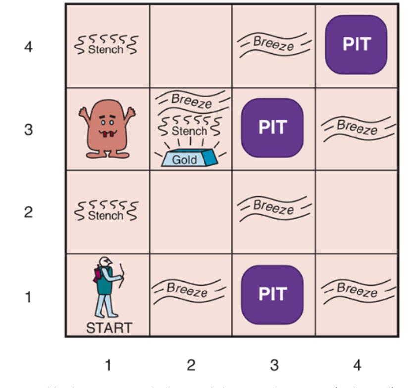
A sample wumpus world is shown in Figure 7.2 . The precise definition of the task environment is given, as suggested in Section 2.3 , by the PEAS description:

• PERFORMANCE MEASURE: for climbing out of the cave with the gold, for falling into a pit or being eaten by the wumpus, for each action taken, and for using up the arrow. The game ends either when the agent dies or when the agent climbs out of the cave.
• ENVIRONMENT: A grid of rooms, with walls surrounding the grid. The agent always starts in the square labeled [1,1], facing to the east. The locations of the gold and the wumpus are chosen randomly, with a uniform distribution, from the squares other than the start square. In addition, each square other than the start can be a pit, with probability 0.2.
• ACTUATORS: The agent can move Forward, TurnLeft by , or TurnRight by . The agent dies a miserable death if it enters a square containing a pit or a live wumpus. (It is safe, albeit smelly, to enter a square with a dead wumpus.) If an agent tries to move forward and bumps into a wall, then the agent does not move. The action Grab can be

used to pick up the gold if it is in the same square as the agent. The action Shoot can be used to fire an arrow in a straight line in the direction the agent is facing. The arrow continues until it either hits (and hence kills) the wumpus or hits a wall. The agent has only one arrow, so only the first Shoot action has any effect. Finally, the action Climb can be used to climb out of the cave, but only from square [1,1].

SENSORS: The agent has five sensors, each of which gives a single bit of information: ‐ In the squares directly (not diagonally) adjacent to the wumpus, the agent will perceive a Stench. 1

1 Presumably the square containing the wumpus also has a stench, but any agent entering that square is eaten before being able to perceive anything.

‐ In the squares directly adjacent to a pit, the agent will perceive a Breeze.

• ‐ In the square where the gold is, the agent will perceive a Glitter.
• ‐ When an agent walks into a wall, it will perceive a Bump.
• ‐ When the wumpus is killed, it emits a woeful Scream that can be perceived anywhere in the cave.

The percepts will be given to the agent program in the form of a list of five symbols; for example, if there is a stench and a breeze, but no glitter, bump, or scream, the agent program will get [Stench,Breeze,None,None,None].

Figure 7.2

We can characterize the wumpus environment along the various dimensions given in Chapter 2 . Clearly, it is deterministic, discrete, static, and single-agent. (The wumpus doesn’t move, fortunately.) It is sequential, because rewards may come only after many actions are taken. It is partially observable, because some aspects of the state are not directly perceivable: the agent’s location, the wumpus’s state of health, and the availability of an arrow. As for the locations of the pits and the wumpus: we could treat them as unobserved parts of the state—in which case, the transition model for the environment is completely known, and finding the locations of pits completes the agent’s knowledge of the state. Alternatively, we could say that the transition model itself is unknown because the agent doesn’t know which Forward actions are fatal—in which case, discovering the locations of pits and wumpus completes the agent’s knowledge of the transition model.

For an agent in the environment, the main challenge is its initial ignorance of the configuration of the environment; overcoming this ignorance seems to require logical reasoning. In most instances of the wumpus world, it is possible for the agent to retrieve the gold safely. Occasionally, the agent must choose between going home empty-handed and risking death to find the gold. About 21% of the environments are utterly unfair, because the gold is in a pit or surrounded by pits.

Let us watch a knowledge-based wumpus agent exploring the environment shown in Figure 7.2 . We use an informal knowledge representation language consisting of writing down symbols in a grid (as in Figures 7.3 and 7.4 ).

1,4	2,4	3,4	4,4	A = Agent B = Breeze G = Glitter, Gold = Safe square OK	1,4	2,4	3,4	4,4
1,3	2,3	3,3	4,3	P = Pit S = Stench V = Visited W = Wumpus	1,3	2,3	3,3	4,3
1,2 OK	2,2	3,2	4,2		1,2 OK	2,2 P?	3,2	4,2
1,1 A OK	2,1 OK	3,1	4,1		1,1 V OK	2,1 A B OK	3,1 P?	4,1
		(a)					(b)

Figure 7.3

The first step taken by the agent in the wumpus world. (a) The initial situation, after percept [None,None,None,None,None]. (b) After moving to [2,1] and perceiving [None,Breeze,None,None,None].

Figure 7.4

1,4	2,4	3,4	4,4	A = Agent B = Breeze G = Glitter, Gold = Safe square OK	1,4	2,4 P?	3,4	4,4
11,3 W!	2,3	3,3	4,3	P = Pit S = Stench V = Visited = Wumpus W	1,3 W!	2,3 A S G B	(3,3 P?	4,3
1,2 ▲ S OK	2,2 OK	3,2	4,2		1,2 S V OK	2,2 V OK	3,2	4,2
1,1 V OK	2,1 B V OK	3,1 P!	4,1		1,1 V OK	2,1 B V OK	3,1 P!	4,1
		(a)					(b)

Two later stages in the progress of the agent. (a) After moving to [1,1] and then [1,2], and perceiving [Stench,None,None,None,None]. (b) After moving to [2,2] and then [2,3], and perceiving [Stench,Breeze,Glitter,None,None].

The agent’s initial knowledge base contains the rules of the environment, as described previously; in particular, it knows that it is in [1,1] and that [1,1] is a safe square; we denote that with an “A” and “OK,” respectively, in square [1,1].

The first percept is [None,None,None,None,None], from which the agent can conclude that its neighboring squares, [1,2] and [2,1], are free of dangers—they are OK. Figure 7.3(a) shows the agent’s state of knowledge at this point.

A cautious agent will move only into a square that it knows to be OK. Let us suppose the agent decides to move forward to [2,1]. The agent perceives a breeze (denoted by “B”) in [2,1], so there must be a pit in a neighboring square. The pit cannot be in [1,1], by the rules of the game, so there must be a pit in [2,2] or [3,1] or both. The notation “P?” in Figure 7.3(b) indicates a possible pit in those squares. At this point, there is only one known square that is OK and that has not yet been visited. So the prudent agent will turn around, go back to [1,1], and then proceed to [1,2].

The agent perceives a stench in [1,2], resulting in the state of knowledge shown in Figure 7.4(a) . The stench in [1,2] means that there must be a wumpus nearby. But the wumpus cannot be in [1,1], by the rules of the game, and it cannot be in [2,2] (or the agent would have detected a stench when it was in [2,1]). Therefore, the agent can infer that the wumpus is in [1,3]. The notation W! indicates this inference. Moreover, the lack of a breeze in [1,2] implies that there is no pit in [2,2]. Yet the agent has already inferred that there must be a pit in either [2,2] or [3,1], so this means it must be in [3,1]. This is a fairly difficult inference, because it combines knowledge gained at different times in different places and relies on the lack of a percept to make one crucial step.

The agent has now proved to itself that there is neither a pit nor a wumpus in [2,2], so it is OK to move there. We do not show the agent’s state of knowledge at [2,2]; we just assume that the agent turns and moves to [2,3], giving us Figure 7.4(b) . In [2,3], the agent detects a glitter, so it should grab the gold and then return home.

Note that in each case for which the agent draws a conclusion from the available information, that conclusion is guaranteed to be correct if the available information is correct. This is a fundamental property of logical reasoning. In the rest of this chapter, we describe how to build logical agents that can represent information and draw conclusions such as those described in the preceding paragraphs.

7.3 Logic

This section summarizes the fundamental concepts of logical representation and reasoning. These beautiful ideas are independent of any of logic’s particular forms. We therefore postpone the technical details of those forms until the next section, using instead the familiar example of ordinary arithmetic.

In Section 7.1 , we said that knowledge bases consist of sentences. These sentences are expressed according to the syntax of the representation language, which specifies all the sentences that are well formed. The notion of syntax is clear enough in ordinary arithmetic: ” ” is a well-formed sentence, whereas ” ” is not.

Syntax

A logic must also define the semantics, or meaning, of sentences. The semantics defines the truth of each sentence with respect to each possible world. For example, the semantics for arithmetic specifies that the sentence ” ” is true in a world where is 2 and is 2, but false in a world where is 1 and is 1. In standard logics, every sentence must be either true or false in each possible world—there is no “in between.” 2

2 Fuzzy logic, discussed in Chapter 13 , allows for degrees of truth.

Semantics

Truth

Possible world

When we need to be precise, we use the term model in place of “possible world.” Whereas possible worlds might be thought of as (potentially) real environments that the agent might or might not be in, models are mathematical abstractions, each of which has a fixed truth value (true or false) for every relevant sentence. Informally, we may think of a possible world as, for example, having men and women sitting at a table playing bridge, and the sentence is true when there are four people in total. Formally, the possible models are just all possible assignments of nonnegative integers to the variables and . Each such assignment determines the truth of any sentence of arithmetic whose variables are and . If a sentence is true in model , we say that satisfies or sometimes is a model of . We use the notation to mean the set of all models of .

Model

Satisfaction

Now that we have a notion of truth, we are ready to talk about logical reasoning. This involves the relation of logical entailment between sentences—the idea that a sentence follows logically from another sentence. In mathematical notation, we write

Entailment

to mean that the sentence entails the sentence . The formal definition of entailment is this: if and only if, in every model in which is true, is also true. Using the notation just introduced, we can write

\[ \alpha = \beta \text{ if and only if } M(\alpha) \subseteq M(\beta) \text{.} \]

(Note the direction of the here: if , then is a stronger assertion than : it rules out more possible worlds.) The relation of entailment is familiar from arithmetic; we are happy with the idea that the sentence entails the sentence . Obviously, in any model where is zero, it is the case that is zero (regardless of the value of ).

We can apply the same kind of analysis to the wumpus-world reasoning example given in the preceding section. Consider the situation in Figure 7.3(b) : the agent has detected nothing in [1,1] and a breeze in [2,1]. These percepts, combined with the agent’s knowledge of the rules of the wumpus world, constitute the KB. The agent is interested in whether the adjacent squares [1,2], [2,2], and [3,1] contain pits. Each of the three squares might or might not contain a pit, so (ignoring other aspects of the world for now) there are possible models. These eight models are shown in Figure 7.5 . 3

3 Although the figure shows the models as partial wumpus worlds, they are really nothing more than assignments of true and false to the sentences “there is a pit in [1,2]” etc. Models, in the mathematical sense, do not need to have ’orrible ’airy wumpuses in them.

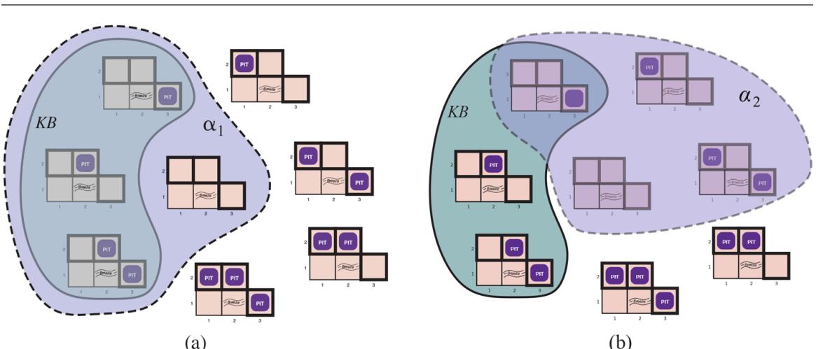
Figure 7.5

Possible models for the presence of pits in squares [1,2], [2,2], and [3,1]. The KB corresponding to the observations of nothing in [1,1] and a breeze in [2,1] is shown by the solid line. (a) Dotted line shows models of (no pit in [1,2]). (b) Dotted line shows models of (no pit in [2,2]).

The KB can be thought of as a set of sentences or as a single sentence that asserts all the individual sentences. The KB is false in models that contradict what the agent knows—for example, the KB is false in any model in which [1,2] contains a pit, because there is no breeze in [1,1]. There are in fact just three models in which the KB is true, and these are shown surrounded by a solid line in Figure 7.5 . Now let us consider two possible conclusions:

We have surrounded the models of and with dotted lines in Figures 7.5(a) and 7.5(b) , respectively. By inspection, we see the following:

Hence, : there is no pit in [1,2]. We can also see that

\[\text{in some models in which } KB \text{ is true, } \alpha\_2 \text{ is false.}\]

Hence, does not entail : the agent cannot conclude that there is no pit in [2,2]. (Nor can it conclude that there is a pit in [2,2].) 4

4 The agent can calculate the probability that there is a pit in [2,2]; Chapter 12 shows how.

The preceding example not only illustrates entailment but also shows how the definition of entailment can be applied to derive conclusions—that is, to carry out logical inference. The inference algorithm illustrated in Figure 7.5 is called model checking, because it enumerates all possible models to check that is true in all models in which is true, that is, that .

Logical inference

Model checking

In understanding entailment and inference, it might help to think of the set of all consequences of as a haystack and of as a needle. Entailment is like the needle being in the haystack; inference is like finding it. This distinction is embodied in some formal notation: if an inference algorithm can derive from , we write

which is pronounced ” is derived from by ” or ” derives from .”

An inference algorithm that derives only entailed sentences is called sound or truthpreserving. Soundness is a highly desirable property. An unsound inference procedure essentially makes things up as it goes along—it announces the discovery of nonexistent needles. It is easy to see that model checking, when it is applicable, is a sound procedure. 5

5 Model checking works if the space of models is finite—for example, in wumpus worlds of fixed size. For arithmetic, on the other hand, the space of models is infinite: even if we restrict ourselves to the integers, there are infinitely many pairs of values for and in the sentence .

Sound

Truth-preserving

The property of completeness is also desirable: an inference algorithm is complete if it can derive any sentence that is entailed. For real haystacks, which are finite in extent, it seems obvious that a systematic examination can always decide whether the needle is in the haystack. For many knowledge bases, however, the haystack of consequences is infinite, and completeness becomes an important issue. Fortunately, there are complete inference procedures for logics that are sufficiently expressive to handle many knowledge bases. 6

6 Compare with the case of infinite search spaces in Chapter 3 , where depth-first search is not complete.

Completeness

We have described a reasoning process whose conclusions are guaranteed to be true in any world in which the premises are true; in particular, if KB is true in the real world, then any sentence derived from KB by a sound inference procedure is also true in the real world. So, while an inference process operates on “syntax”—internal physical configurations such as bits in registers or patterns of electrical blips in brains—the process corresponds to the real-world relationship whereby some aspect of the real world is the case by virtue of other aspects of the real world being the case. This correspondence between world and representation is illustrated in Figure 7.6 . 7

7 As Wittgenstein (1922) put it in his famous Tractatus: “The world is everything that is the case.”

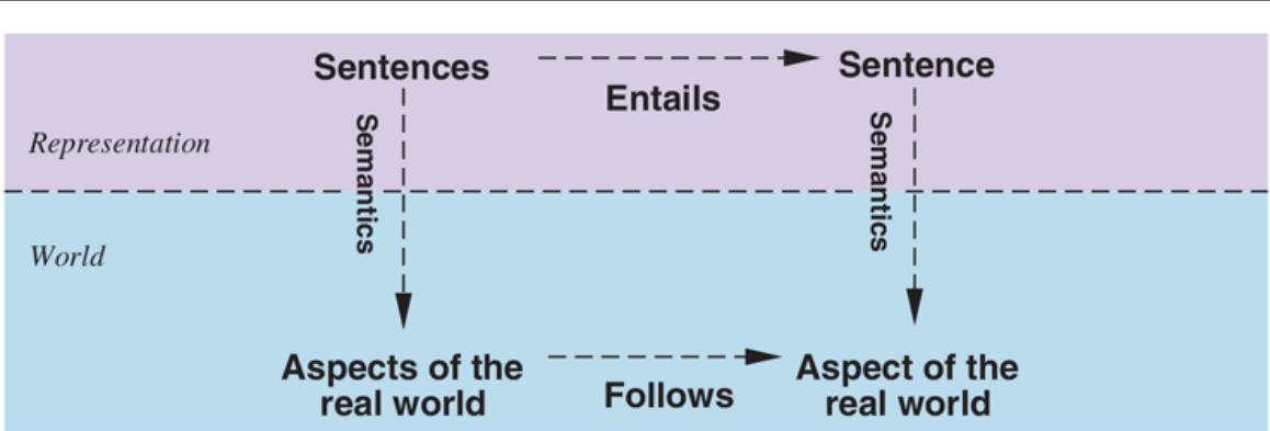
Figure 7.6

Sentences are physical configurations of the agent, and reasoning is a process of constructing new physical configurations from old ones. Logical reasoning should ensure that the new configurations represent aspects of the world that actually follow from the aspects that the old configurations represent.

The final issue to consider is grounding—the connection between logical reasoning processes and the real environment in which the agent exists. In particular, how do we know that is true in the real world? (After all, is just “syntax” inside the agent’s head.) This is a philosophical question about which many, many books have been written. (See Chapter 27 .) A simple answer is that the agent’s sensors create the connection. For example, our wumpus-world agent has a smell sensor. The agent program creates a suitable sentence whenever there is a smell. Then, whenever that sentence is in the knowledge base, it is true in the real world. Thus, the meaning and truth of percept sentences are defined by the processes of sensing and sentence construction that produce them. What about the rest of the agent’s knowledge, such as its belief that wumpuses cause smells in adjacent squares? This is not a direct representation of a single percept, but a general rule—derived, perhaps, from perceptual experience but not identical to a statement of that experience. General rules like this are produced by a sentence construction process called learning, which is the subject of Part V. Learning is fallible. It could be the case that wumpuses cause smells except on February 29 in leap years, which is when they take their baths. Thus, may not be true in the real world, but with good learning procedures, there is reason for optimism.

Grounding

7.4 Propositional Logic: A Very Simple Logic

We now present propositional logic. We describe its syntax (the structure of sentences) and its semantics (the way in which the truth of sentences is determined). From these, we derive a simple, syntactic algorithm for logical inference that implements the semantic notion of entailment. Everything takes place, of course, in the wumpus world.

Propositional logic

7.4.1 Syntax

The syntax of propositional logic defines the allowable sentences. The atomic sentences consist of a single proposition symbol. Each such symbol stands for a proposition that can be true or false. We use symbols that start with an uppercase letter and may contain other letters or subscripts, for example: , , , , and FacingEast. The names are arbitrary but are often chosen to have some mnemonic value—we use to stand for the proposition that the wumpus is in [1,3]. (Remember that symbols such as are atomic, i.e., , 1, and 3 are not meaningful parts of the symbol.) There are two proposition symbols with fixed meanings: True is the always-true proposition and False is the always-false proposition. Complex sentences are constructed from simpler sentences, using parentheses and operators called logical connectives. There are five connectives in common use:

Atomic sentences

Proposition symbol

Complex sentences

Logical connectives

(not). A sentence such as is called the negation of . A literal is either an atomic sentence (a positive literal) or a negated atomic sentence (a negative literal).

Negation

Literal

(and). A sentence whose main connective is , such as , is called a conjunction; its parts are the conjuncts. (The looks like an “A” for “And.”)

Conjunction

(or). A sentence whose main connective is , such as , is a disjunction; its parts are disjuncts—in this example, and .

Disjunction

(implies). A sentence such as is called an implication (or conditional). Its premise or antecedent is , and its conclusion or consequent is . Implications are also known as rules or if–then statements. The implication symbol is sometimes written in other books as or .

Implication
Premise
Conclusion
Rules

(if and only if). The sentence is a biconditional.

Biconditional

Figure 7.7 gives a formal grammar of propositional logic. (BNF notation is explained on page 1030.) The BNF grammar is augmented with an operator precedence list to remove ambiguity when multiple operators are used. The “not” operator has the highest precedence, which means that in the sentence the binds most tightly, giving us the equivalent of rather than . (The notation for ordinary arithmetic is the same: is 2, not –6.) When appropriate, we also use parentheses and square brackets to clarify the intended sentence structure and improve readability.

Figure 7.7

A BNF (Backus–Naur Form) grammar of sentences in propositional logic, along with operator precedences, from highest to lowest.

7.4.2 Semantics

Having specified the syntax of propositional logic, we now specify its semantics. The semantics defines the rules for determining the truth of a sentence with respect to a particular model. In propositional logic, a model simply sets the truth value—true or false for every proposition symbol. For example, if the sentences in the knowledge base make use of the proposition symbols , and , then one possible model is

\[m\_1 = \{P\_{1,2} = false, P\_{2,2} = false, P\_{3,1} = true\}.\]

Truth value

With three proposition symbols, there are possible models—exactly those depicted in Figure 7.5 . Notice, however, that the models are purely mathematical objects with no necessary connection to wumpus worlds. is just a symbol; it might mean “there is a pit in [1,2]” or “I’m in Paris today and tomorrow.”

The semantics for propositional logic must specify how to compute the truth value of any sentence, given a model. This is done recursively. All sentences are constructed from atomic sentences and the five connectives; therefore, we need to specify how to compute the truth of atomic sentences and how to compute the truth of sentences formed with each of the five connectives. Atomic sentences are easy:

• True is true in every model and False is false in every model.
• The truth value of every other proposition symbol must be specified directly in the model. For example, in the model given earlier, is false.

For complex sentences, we have five rules, which hold for any subsentences and (atomic or complex) in any model (here “iff” means “if and only if”):

• is true iff is false in .
• is true iff both and are true in .
• is true iff either or is true in .
• is true unless is true and is false in .
• is true iff and are both true or both false in .

The rules can also be expressed with truth tables that specify the truth value of a complex sentence for each possible assignment of truth values to its components. Truth tables for the five connectives are given in Figure 7.8 . From these tables, the truth value of any sentence can be computed with respect to any model by a simple recursive evaluation. For example, the sentence , evaluated in , gives . Exercise 7.TRUV asks you to write the algorithm PL-TRUE? which computes the truth value of a propositional logic sentence in a model .

P	Q	-P	PAQ	PVQ	P = Q =	P & Q
false	false	true	false	false	true	true
false	true	true	false	true	true	false
true	false	false	false	true	false	false
true	true	false	true	true	true	true

Truth tables for the five logical connectives. To use the table to compute, for example, the value of when is true and is false, first look on the left for the row where is true and is false (the third row). Then look in that row under the column to see the result: true.

Truth table

The truth tables for “and,” “or,” and “not” are in close accord with our intuitions about the English words. The main point of possible confusion is that is true when is true or is true or both. A different connective, called “exclusive or” (“xor” for short), yields false when both disjuncts are true. There is no consensus on the symbol for exclusive or; some choices are or or . 8

8 Latin uses two separate words: “vel” is inclusive or and “aut” is exclusive or.

The truth table for may not quite fit one’s intuitive understanding of ” implies ” or “if then .” For one thing, propositional logic does not require any relation of causation or relevance between and . The sentence “5 is odd implies Tokyo is the capital of Japan” is a true sentence of propositional logic (under the normal interpretation), even though it is a decidedly odd sentence of English. Another point of confusion is that any implication is true whenever its antecedent is false. For example, “5 is even implies Sam is smart” is true, regardless of whether Sam is smart. This seems bizarre, but it makes sense if you think of ” ” as saying, “If is true, then I am claiming that is true; otherwise I am making no claim.” The only way for this sentence to be false is if is true but is false.

The biconditional, , is true whenever both and are true. In English, this is often written as ” if and only if .” Many of the rules of the wumpus world are best written using . For example, a square is breezy if a neighboring square has a pit, and a square is breezy only if a neighboring square has a pit. So we need a biconditional,

\[B\_{1,1} \Leftrightarrow (P\_{1,2} \lor P\_{2,1})\]

where means that there is a breeze in [1,1].

7.4.3 A simple knowledge base

Now that we have defined the semantics for propositional logic, we can construct a knowledge base for the wumpus world. We focus first on the immutable aspects of the wumpus world, leaving the mutable aspects for a later section. For now, we need the following symbols for each location:

• is true if there is a pit in .
• is true if there is a wumpus in , dead or alive.
• is true if there is a breeze in .
• is true if there is a stench in .
• is true if the agent is in location .

The sentences we write will suffice to derive (there is no pit in [1,2]), as was done informally in Section 7.3 . We label each sentence so that we can refer to them:

There is no pit in [1,1]:

\[R\_1: \quad \neg P\_{1,1} \dots\]

A square is breezy if and only if there is a pit in a neighboring square. This has to be stated for each square; for now, we include just the relevant squares:

\[\begin{aligned} R\_2: &\quad B\_{1,1} \Leftrightarrow \left(P\_{1,2} \vee P\_{2,1}\right). \\ R\_3: &\quad B\_{2,1} \Leftrightarrow \left(P\_{1,1} \vee P\_{2,2} \vee P\_{3,1}\right). \end{aligned}\]

The preceding sentences are true in all wumpus worlds. Now we include the breeze percepts for the first two squares visited in the specific world the agent is in, leading up to the situation in Figure 7.3(b) .

7.4.4 A simple inference procedure

Our goal now is to decide whether for some sentence . For example, is entailed by our ? Our first algorithm for inference is a model-checking approach that is a direct implementation of the definition of entailment: enumerate the models, and check that is true in every model in which is true. Models are assignments of true or false to every proposition symbol. Returning to our wumpus-world example, the relevant proposition symbols are , , , , , , and . With seven symbols, there are possible models; in three of these, is true (Figure 7.9 ). In those three models, is true, hence there is no pit in [1,2]. On the other hand, is true in two of the three models and false in one, so we cannot yet tell whether there is a pit in [2,2].

Figure 7.9

B1,1	B2,1	P1,1	P1,2	P2,1	P2,2	P3.1	R1	R2	R3	R4	R5	KB
false	false	false	false	false	false	false	true	true	true	true	false	false
false	false	false	false	false	false	true	true	true	false	true	false	false
false	true	false	false	false	false	false	true	true	false	true	true	false
false	true	false	false	false	false	true	true	true	true	true	true	true
false	true	false	false	false	true	false	true	true	true	true	true	true
false	true	false	false	false	true	true	true	true	true	true	true	true
false	true	false	false	true	false	false	true	false	false	true	true	false
true	true	true	true	true	true	true	false	true	true	false	true	false

A truth table constructed for the knowledge base given in the text. is true if through are true, which occurs in just 3 of the 128 rows (the ones underlined in the right-hand column). In all 3 rows, is false, so there is no pit in [1,2]. On the other hand, there might (or might not) be a pit in [2,2].

Figure 7.9 reproduces in a more precise form the reasoning illustrated in Figure 7.5 . A general algorithm for deciding entailment in propositional logic is shown in Figure 7.10 . Like the BACKTRACKING-SEARCH algorithm on page 192, TT-ENTAILS? performs a recursive enumeration of a finite space of assignments to symbols. The algorithm is sound because it implements directly the definition of entailment, and complete because it works for any and and always terminates—there are only finitely many models to examine.

A truth-table enumeration algorithm for deciding propositional entailment. (TT stands for truth table.) PL-TRUE? returns true if a sentence holds within a model. The variable model represents a partial model an assignment to some of the symbols. The keyword and here is an infix function symbol in the pseudocode programming language, not an operator in proposition logic; it takes two arguments and returns true or false.

Of course, “finitely many” is not always the same as “few.” If and contain symbols in all, then there are models. Thus, the time complexity of the algorithm is . (The space complexity is only because the enumeration is depth-first.) Later in this chapter we show algorithms that are much more efficient in many cases. Unfortunately, propositional entailment is co-NP-complete (i.e., probably no easier than NP-complete—see Appendix A ), so every known inference algorithm for propositional logic has a worst-case complexity that is exponential in the size of the input.

7.5 Propositional Theorem Proving

So far, we have shown how to determine entailment by model checking: enumerating models and showing that the sentence must hold in all models. In this section, we show how entailment can be done by theorem proving—applying rules of inference directly to the sentences in our knowledge base to construct a proof of the desired sentence without consulting models. If the number of models is large but the length of the proof is short, then theorem proving can be more efficient than model checking.

Theorem proving

Before we plunge into the details of theorem-proving algorithms, we will need some additional concepts related to entailment. The first concept is logical equivalence: two sentences and are logically equivalent if they are true in the same set of models. We write this as (Note that is used to make claims about sentences, while is used as part of a sentence.) For example, we can easily show (using truth tables) that and are logically equivalent; other equivalences are shown in Figure 7.11 . These equivalences play much the same role in logic as arithmetic identities do in ordinary mathematics. An alternative definition of equivalence is as follows: any two sentences and are equivalent if and only if each of them entails the other:

\[ \alpha \equiv \beta \quad \text{if and only if} \quad \alpha \vdash \beta \text{ and } \beta \vdash \alpha \text{ .} \]

Figure 7.11

\[\begin{array}{rcl} (\alpha \land \beta) & \equiv & (\beta \land \alpha) \quad \text{commutativity of } \land \\ (\alpha \lor \beta) & \equiv (\beta \lor \alpha) \quad \text{commutativity of } \lor \\ ( (\alpha \land \beta) \land \gamma) & \equiv & (\alpha \land (\beta \land \gamma)) \quad \text{associativity of } \land \\ ( (\alpha \lor \beta) \lor \gamma) & \equiv & (\alpha \lor (\beta \lor \gamma)) \quad \text{associativity of } \lor \\ & \neg(\neg \alpha) & \equiv \alpha \quad \text{double-negation elimination} \\ ( \alpha \to \beta) & \equiv & (\neg \beta \Rightarrow \neg \alpha) \quad \text{contrapsposition} \\ ( \alpha \to \beta) & \equiv & (\neg \alpha \lor \beta) \quad \text{implication elimination} \\ ( \alpha \to \beta) & \equiv & ((\alpha \to \beta) \land (\beta \Rightarrow \alpha)) \quad \text{bicconditional elimination} \\ \neg( \alpha \land \beta) & \equiv & (\neg \alpha \lor \neg \beta) \quad \text{De Morgan} \\ \neg( \alpha \lor \beta) & \equiv & (\neg \alpha \land \neg \beta) \quad \text{De Morgan} \\ ( \alpha \land (\beta \lor \gamma)) & \equiv & ((\alpha \land \beta) \lor (\alpha \land \gamma)) \quad \text{disitivity of } \land \text{ over } \land \\ ( \alpha \lor (\beta \lor \gamma)) & \equiv & ((\alpha \lor \beta) \land (\alpha \lor \gamma)) \quad \text{disitivity of } \lor \text{ over } \land \end{array}\]

Standard logical equivalences. The symbols , , and stand for arbitrary sentences of propositional logic.

Logical equivalence

The second concept we will need is validity. A sentence is valid if it is true in all models. For example, the sentence is valid. Valid sentences are also known as tautologies—they are necessarily true. Because the sentence True is true in all models, every valid sentence is logically equivalent to True. What good are valid sentences? From our definition of entailment, we can derive the deduction theorem, which was known to the ancient Greeks:

For any sentences and , if and only if the sentence is valid.

Validity

Tautology

Deduction theorem

(Exercise 7.DEDU asks for a proof.) Hence, we can decide if by checking that is true in every model—which is essentially what the inference algorithm in Figure 7.10 does —or by proving that is equivalent to True. Conversely, the deduction theorem states that every valid implication sentence describes a legitimate inference.

Satisfiability

The final concept we will need is satisfiability. A sentence is satisfiable if it is true in, or satisfied by, some model. For example, the knowledge base given earlier, ( ), is satisfiable because there are three models in which it is true, as shown in Figure 7.9 . Satisfiability can be checked by enumerating the possible models until one is found that satisfies the sentence. The problem of determining the satisfiability of sentences in propositional logic—the SAT problem—was the first problem proved to be NPcomplete. Many problems in computer science are really satisfiability problems. For example, all the constraint satisfaction problems in Chapter 6 ask whether the constraints are satisfiable by some assignment.

SAT

Validity and satisfiability are of course connected: is valid iff is unsatisfiable; contrapositively, is satisfiable iff is not valid. We also have the following useful result:

if and only if the sentence is unsatisfiable.

Proving from by checking the unsatisfiability of corresponds exactly to the standard mathematical proof technique of reductio ad absurdum (literally, “reduction to an absurd thing”). It is also called proof by refutation or proof by contradiction. One assumes a sentence to be false and shows that this leads to a contradiction with known axioms . This contradiction is exactly what is meant by saying that the sentence is unsatisfiable.

Reductio ad absurdum

Refutation

Contradiction

7.5.1 Inference and proofs

This section covers inference rules that can be applied to derive a proof—a chain of conclusions that leads to the desired goal. The best-known rule is called Modus Ponens (Latin for mode that affirms) and is written

\[\frac{\alpha \Rightarrow \beta, \quad \alpha}{\beta}\]

Inference rules

Proof

Modus Ponens

The notation means that, whenever any sentences of the form and are given, then the sentence can be inferred. For example, if and are given, then Shoot can be inferred.

Another useful inference rule is And-Elimination, which says that, from a conjunction, any of the conjuncts can be inferred:

\[\frac{\alpha \wedge \beta}{\alpha} \,.\]

And-Elimination

For example, from , WumpusAlive can be inferred.

By considering the possible truth values of and , one can easily show once and for all that Modus Ponens and And-Elimination are sound. These rules can then be used in any particular instances where they apply, generating sound inferences without the need for enumerating models.

All of the logical equivalences in Figure 7.11 can be used as inference rules. For example, the equivalence for biconditional elimination yields the two inference rules

\[\begin{array}{c} \alpha \Leftrightarrow \beta\\ \hline (\alpha \Rightarrow \beta) \land (\beta \Rightarrow \alpha) \end{array} \quad \text{and} \quad \begin{array}{c} (\alpha \Rightarrow \beta) \land (\beta \Rightarrow \alpha) \\ \hline \alpha \Leftrightarrow \beta \end{array} .\]

Not all inference rules work in both directions like this. For example, we cannot run Modus Ponens in the opposite direction to obtain and from .

Let us see how these inference rules and equivalences can be used in the wumpus world. We start with the knowledge base containing through and show how to prove , that is, there is no pit in [1,2]:

1. Apply biconditional elimination to to obtain

\[R\_6: \quad \left(B\_{1,1} \Rightarrow \left(P\_{1,2} \lor P\_{2,1}\right)\right) \land \left(\left(P\_{1,2} \lor P\_{2,1}\right) \Rightarrow B\_{1,1}\right) \dots\]

2. Apply And-Elimination to to obtain

\[R\_7: \quad \left( (P\_{1,2} \lor P\_{2,1}) \Rightarrow B\_{1,1} \right).\]

3. Logical equivalence for contrapositives gives

\[R\_8: \quad \left(\neg B\_{1,1} \Rightarrow \neg (P\_{1,2} \lor P\_{2,1})\right) .\]

4. Apply Modus Ponens with and the percept (i.e., ), to obtain

\[R\_{\emptyset}: \quad \neg (P\_{1,2} \lor P\_{2,1}) \; .\]

5. Apply De Morgan’s rule, giving the conclusion

\[R\_{10}: \quad \neg P\_{1,2} \land \neg P\_{2,1} \dots\]

That is, neither [1,2] nor [2,1] contains a pit.

Any of the search algorithms in Chapter 3 can be used to find a sequence of steps that constitutes a proof like this. We just need to define a proof problem as follows:

• INITIAL STATE: the initial knowledge base.
• ACTIONS: the set of actions consists of all the inference rules applied to all the sentences that match the top half of the inference rule.
• RESULT: the result of an action is to add the sentence in the bottom half of the inference rule.
• GOAL: the goal is a state that contains the sentence we are trying to prove.

Thus, searching for proofs is an alternative to enumerating models. In many practical cases finding a proof can be more efficient because the proof can ignore irrelevant propositions, no matter how many of them there are. For example, the proof just given leading to does not mention the propositions They can be ignored because the goal proposition, , appears only in sentence ; appear only in and so , , and have no bearing on the proof. The same would hold even if we added a million more sentences to the knowledge base; the simple truth-table algorithm, on the other hand, would be overwhelmed by the exponential explosion of models.

One final property of logical systems is monotonicity, which says that the set of entailed sentences can only increase as information is added to the knowledge base. For any sentences and , 9

9 Nonmonotonic logics, which violate the monotonicity property, capture a common property of human reasoning: changing one’s mind. They are discussed in Section 10.6 .

Monotonicity

For example, suppose the knowledge base contains the additional assertion stating that there are exactly eight pits in the world. This knowledge might help the agent draw additional conclusions, but it cannot invalidate any conclusion already inferred—such as the conclusion that there is no pit in [1,2]. Monotonicity means that inference rules can be applied whenever suitable premises are found in the knowledge base—the conclusion of the rule must follow regardless of what else is in the knowledge base.

7.5.2 Proof by resolution

We have argued that the inference rules covered so far are sound, but we have not discussed the question of completeness for the inference algorithms that use them. Search algorithms such as iterative deepening search (page 81) are complete in the sense that they will find any reachable goal, but if the available inference rules are inadequate, then the goal is not reachable—no proof exists that uses only those inference rules. For example, if we removed

the biconditional elimination rule, the proof in the preceding section would not go through. The current section introduces a single inference rule, resolution, that yields a complete inference algorithm when coupled with any complete search algorithm.

We begin by using a simple version of the resolution rule in the wumpus world. Let us consider the steps leading up to Figure 7.4(a) : the agent returns from [2,1] to [1,1] and then goes to [1,2], where it perceives a stench, but no breeze. We add the following facts to the knowledge base:

\[\begin{aligned} R\_{11}: &\quad \neg B\_{1,2}.\\ R\_{12}: &\quad B\_{1,2} \Leftrightarrow (P\_{1,1} \lor P\_{2,2} \lor P\_{1,3}) \end{aligned}\]

By the same process that led to earlier, we can now derive the absence of pits in [2,2] and [1,3] (remember that [1,1] is already known to be pitless):

\[\begin{array}{rcl} R\_{13}: & \neg P\_{2,2}. \\ R\_{14}: & \neg P\_{1,3}. \end{array}\]

We can also apply biconditional elimination to , followed by Modus Ponens with , to obtain the fact that there is a pit in [1,1], [2,2], or [3,1]:

\[R\_{15}: \quad P\_{1,1} \lor P\_{2,2} \lor P\_{3,1} \dots\]

Now comes the first application of the resolution rule: the literal in resolves with the literal in to give the resolvent

\[R\_{16}: \quad P\_{1,1} \lor P\_{3,1} \cdot\]

Resolvent

In English; if there’s a pit in one of [1,1], [2,2], and [3,1] and it’s not in [2,2], then it’s in [1,1] or [3,1]. Similarly, the literal in resolves with the literal in to give

\[R\_{17}: \quad P\_{3,1} \dots\]

In English: if there’s a pit in [1,1] or [3,1] and it’s not in [1,1], then it’s in [3,1]. These last two inference steps are examples of the unit resolution inference rule

\[\frac{\ell\_1 \vee \dots \vee \ell\_k, \qquad m}{\ell\_1 \vee \dots \vee \ell\_{i-1} \vee \ell\_{i+1} \vee \dots \vee \ell\_k}\]

Unit resolution

where each is a literal and and are complementary literals (i.e., one is the negation of the other). Thus, the unit resolution rule takes a clause—a disjunction of literals—and a literal and produces a new clause. Note that a single literal can be viewed as a disjunction of one literal, also known as a unit clause.

Complementary literals

Clause

Unit clause

The unit resolution rule can be generalized to the full resolution rule

\[\frac{\ell\_1 \lor \cdots \lor \ell\_k, \qquad m\_1 \lor \cdots \lor m\_n}{\ell\_1 \lor \cdots \lor \ell\_{i-1} \lor \ell\_{i+1} \lor \cdots \lor \ell\_k \lor m\_1 \lor \cdots \lor m\_{j-1} \lor m\_{j+1} \lor \cdots \lor m\_n}\]

Resolution

where and are complementary literals. This says that resolution takes two clauses and produces a new clause containing all the literals of the two original clauses except the two complementary literals. For example, we have

\[\frac{P\_{1,1} \lor P\_{3,1}, \qquad \neg P\_{1,1} \lor \neg P\_{2,2}}{P\_{3,1} \lor \neg P\_{2,2}}\]

You can resolve only one pair of complementary literals at a time. For example, we can resolve and to deduce

\[ \frac{P \lor \neg Q \lor R}{\neg Q \lor Q \lor R}, \]

but you can’t resolve on both and at once to infer . There is one more technical aspect of the resolution rule: the resulting clause should contain only one copy of each literal. The removal of multiple copies of literals is called factoring. For example, if we resolve with , we obtain , which is reduced to just by factoring. 10

10 If a clause is viewed as a set of literals, then this restriction is automatically respected. Using set notation for clauses makes the resolution rule much cleaner, at the cost of introducing additional notation.

Factoring

The soundness of the resolution rule can be seen easily by considering the literal that is complementary to literal in the other clause. If is true, then is false, and hence must be true, because is given. If is false, then must be true because is given. Now is either true or false, so one or other of these conclusions holds—exactly as the resolution rule states.

What is more surprising about the resolution rule is that it forms the basis for a family of complete inference procedures. A resolution-based theorem prover can, for any sentences and in propositional logic, decide whether . The next two subsections explain how resolution accomplishes this.

Conjunctive normal form

The resolution rule applies only to clauses (that is, disjunctions of literals), so it would seem to be relevant only to knowledge bases and queries consisting of clauses. How, then, can it lead to a complete inference procedure for all of propositional logic? The answer is that every sentence of propositional logic is logically equivalent to a conjunction of clauses.

A sentence expressed as a conjunction of clauses is said to be in conjunctive normal form or CNF (see Figure 7.12 ). We now describe a procedure for converting to CNF. We illustrate the procedure by converting the sentence into CNF. The steps are as follows:

Conjunctive normal form

CNF

1. Eliminate , replacing with .

\[(B\_{1,1} \Rightarrow (P\_{1,2} \lor P\_{2,1})) \land ((P\_{1,2} \lor P\_{2,1}) \Rightarrow B\_{1,1}) \dots\]

2. Eliminate , replacing with :

\[(\neg B\_{1,1} \lor P\_{1,2} \lor P\_{2,1}) \land (\neg (P\_{1,2} \lor P\_{2,1}) \lor B\_{1,1}) \; .\]

3. CNF requires to appear only in literals, so we “move inwards” by repeated application of the following equivalences from Figure 7.11 :

(double-negation elimination)

(De Morgan) (De Morgan)

In the example, we require just one application of the last rule:

\[(\neg B\_{1,1} \lor P\_{1,2} \lor P\_{2,1}) \land ((\neg P\_{1,2} \land \neg P\_{2,1}) \lor B\_{1,1}) \dots\]

4. Now we have a sentence containing nested and operators applied to literals. We apply the distributivity law from Figure 7.11 , distributing over wherever possible.

\[(\neg B\_{1,1} \lor P\_{1,2} \lor P\_{2,1}) \land (\neg P\_{1,2} \lor B\_{1,1}) \land (\neg P\_{2,1} \lor B\_{1,1}) \; .\]

Figure 7.12

	CNFSentence > Clause1 ^ Clausen
	Clause -> Literal V V Literalm
	Fact > Symbol
	Literal -> Symbol -Symbol
	Symbol > P Q R
	HornClauseForm -> DefiniteClauseForm GoalClauseForm
	DefiniteClauseForm -> Fact (Symbol ^ ·· · · Symbol => Symbol
	GoalClauseForm -> (Symbol1 /··· · · Symbol;) => False

A grammar for conjunctive normal form, Horn clauses, and definite clauses. A CNF clause such as can be written in definite clause form as

The original sentence is now in CNF, as a conjunction of three clauses. It is much harder to read, but it can be used as input to a resolution procedure.

A resolution algorithm

Inference procedures based on resolution work by using the principle of proof by contradiction introduced on page 223 . That is, to show that , we show that is unsatisfiable. We do this by proving a contradiction.

A resolution algorithm is shown in Figure 7.13 . First, is converted into CNF. Then, the resolution rule is applied to the resulting clauses. Each pair that contains

complementary literals is resolved to produce a new clause, which is added to the set if it is not already present. The process continues until one of two things happens:

• there are no new clauses that can be added, in which case does not entail ; or,
• two clauses resolve to yield the empty clause, in which case entails .

Figure 7.13

A simple resolution algorithm for propositional logic. PL-RESOLVE returns the set of all possible clauses obtained by resolving its two inputs.

The empty clause—a disjunction of no disjuncts—is equivalent to False because a disjunction is true only if at least one of its disjuncts is true. Moreover, the empty clause arises only from resolving two contradictory unit clauses such as and .

We can apply the resolution procedure to a very simple inference in the wumpus world. When the agent is in [1,1], there is no breeze, so there can be no pits in neighboring squares. The relevant knowledge base is

\[KB = R\_2 \land R\_4 = (B\_{1,1} \Leftrightarrow (P\_{1,2} \lor P\_{2,1})) \land \neg B\_{1,1}\]

and we wish to prove , which is, say, . When we convert into CNF, we obtain the clauses shown at the top of Figure 7.14 . The second row of the figure shows clauses obtained by resolving pairs in the first row. Then, when is resolved with , we obtain the empty clause, shown as a small square. Inspection of Figure 7.14 reveals

that many resolution steps are pointless. For example, the clause is equivalent to which is equivalent to True. Deducing that True is true is not very helpful. Therefore, any clause in which two complementary literals appear can be discarded.

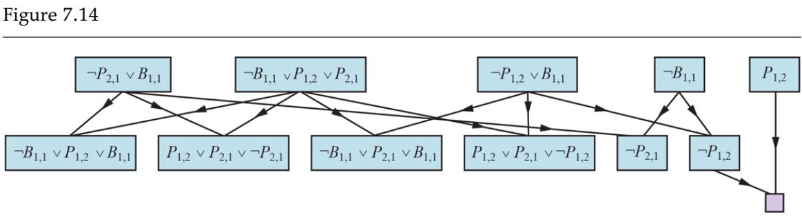
Partial application of PL-RESOLUTION to a simple inference in the wumpus world to prove the query Each of the leftmost four clauses in the top row is paired with each of the other three, and the resolution rule is applied to yield the clauses on the bottom row. We see that the third and fourth clauses on the top row combine to yield the clause which is then resolved with to yield the empty clause, meaning that the query is proven.

Completeness of resolution

To conclude our discussion of resolution, we now show why PL-RESOLUTION is complete. To do this, we introduce the resolution closure RC(S) of a set of clauses , which is the set of all clauses derivable by repeated application of the resolution rule to clauses in or their derivatives. The resolution closure is what PL-RESOLUTION computes as the final value of the variable clauses. It is easy to see that RC(S) must be finite: thanks to the factoring step, there are only finitely many distinct clauses that can be constructed out of the symbols that appear in . Hence, PL-RESOLUTION always terminates.

Resolution closure

The completeness theorem for resolution in propositional logic is called the ground resolution theorem:

If a set of clauses is unsatisfiable, then the resolution closure of those clauses contains the empty clause.

Ground resolution theorem

This theorem is proved by demonstrating its contrapositive: if the closure RC(S) does not contain the empty clause, then is satisfiable. In fact, we can construct a model for with suitable truth values for . The construction procedure is as follows:

For from 1 to ,

• If a clause in RC(S) contains the literal and all its other literals are false under the assignment chosen for , then assign false to . - Otherwise, assign true to .

This assignment to is a model of . To see this, assume the opposite—that, at some stage in the sequence, assigning symbol causes some clause to become false. For this to happen, it must be the case that all the other literals in must already have been falsified by assignments to . Thus, must now look like either or like . If just one of these two is in RC(S), then the algorithm will assign the appropriate truth value to to make true, so can only be falsified if both of these clauses are in RC(S).

Now, since RC(S) is closed under resolution, it will contain the resolvent of these two clauses, and that resolvent will have all of its literals already falsified by the assignments to . This contradicts our assumption that the first falsified clause appears at stage . Hence, we have proved that the construction never falsifies a clause in RC(S); that is, it produces a model of RC(S). Finally, because is contained in RC(S), any model of RC(S) is a model of itself.

7.5.3 Horn clauses and definite clauses

The completeness of resolution makes it a very important inference method. In many practical situations, however, the full power of resolution is not needed. Some real-world knowledge bases satisfy certain restrictions on the form of sentences they contain, which enables them to use a more restricted and efficient inference algorithm.

One such restricted form is the definite clause, which is a disjunction of literals of which exactly one is positive. For example, the clause is a definite clause, whereas is not, because it has two positive clauses.

Definite clause

Slightly more general is the Horn clause, which is a disjunction of literals of which at most one is positive. So all definite clauses are Horn clauses, as are clauses with no positive literals; these are called goal clauses. Horn clauses are closed under resolution: if you resolve two Horn clauses, you get back a Horn clause. One more class is the k-CNF sentence, which is a CNF sentence where each clause has at most k literals.

Horn clause

Goal clauses

Knowledge bases containing only definite clauses are interesting for three reasons:

1. Every definite clause can be written as an implication whose premise is a conjunction of positive literals and whose conclusion is a single positive literal. (See Exercise 7.DISJ.) For example, the definite clause can be written as the implication . In the implication form, the sentence is easier to understand: it says that if the agent is in [1,1] and there is a breeze percept, then [1,1] is breezy. In Horn form, the premise is called the body and the conclusion is called the head. A sentence consisting of a single positive literal, such as , is called a fact. It too can be written in implication form as , but it is simpler to write just .

Body
Head
Fact

2. Inference with Horn clauses can be done through the forward-chaining and backward-chaining algorithms, which we explain next. Both of these algorithms are natural, in that the inference steps are obvious and easy for humans to follow. This type of inference is the basis for logic programming, which is discussed in Chapter 9 .

Forward-chaining

Backward-chaining

3. Deciding entailment with Horn clauses can be done in time that is linear in the size of the knowledge base—a pleasant surprise.

7.5.4 Forward and backward chaining

The forward-chaining algorithm PL-FC-ENTAILS? determines if a single proposition symbol —the query—is entailed by a knowledge base of definite clauses. It begins from known facts (positive literals) in the knowledge base. If all the premises of an implication are known, then its conclusion is added to the set of known facts. For example, if and Breeze are known and is in the knowledge base, then can be added. This process continues until the query q is added or until no further inferences can be made. The algorithm is shown in Figure 7.15 ; the main point to remember is that it runs in linear time.

Figure 7.15

The forward-chaining algorithm for propositional logic. The agenda keeps track of symbols known to be true but not yet “processed.” The count table keeps track of how many premises of each implication are not yet proven. Whenever a new symbol from the agenda is processed, the count is reduced by one for each implication in whose premise appears (easily identified in constant time with appropriate indexing.) If a count reaches zero, all the premises of the implication are known, so its conclusion can be added to the agenda. Finally, we need to keep track of which symbols have been processed; a symbol that is already in the set of inferred symbols need not be added to the agenda again. This avoids redundant work and prevents loops caused by implications such as and .

The best way to understand the algorithm is through an example and a picture. Figure 7.16(a) shows a simple knowledge base of Horn clauses with and as known facts. Figure 7.16(b) shows the same knowledge base drawn as an AND–OR graph (see Chapter 4 ). In AND–OR graphs, multiple edges joined by an arc indicate a conjunction—every edge must be proved—while multiple edges without an arc indicate a disjunction—any edge can be proved. It is easy to see how forward chaining works in the graph. The known leaves (here, and ) are set, and inference propagates up the graph as far as possible. Wherever a conjunction appears, the propagation waits until all the conjuncts are known before proceeding. The reader is encouraged to work through the example in detail.

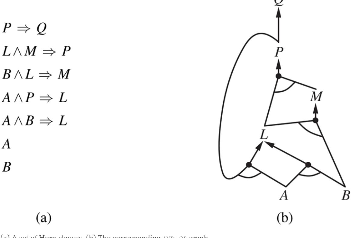
⁽a) A set of Horn clauses. (b) The corresponding AND–OR graph.

It is easy to see that forward chaining is sound: every inference is essentially an application of Modus Ponens. Forward chaining is also complete: every entailed atomic sentence will be derived. The easiest way to see this is to consider the final state of the inferred table (after the algorithm reaches a fixed point where no new inferences are possible). The table contains true for each symbol inferred during the process, and false for all other symbols. We can view the table as a logical model; moreover, every definite clause in the original KB is true in this model.

To see this, assume the opposite, namely that some clause is false in the model. Then must be true in the model and must be false in the model. But this contradicts our assumption that the algorithm has reached a fixed point, because we would now be licensed to add to the KB. We can conclude, therefore, that the set of atomic sentences inferred at the fixed point defines a model of the original KB. Furthermore, any atomic sentence that is entailed by the KB must be true in all its models and in this model in particular. Hence, every entailed atomic sentence must be inferred by the algorithm.

Forward chaining is an example of the general concept of data-driven reasoning—that is, reasoning in which the focus of attention starts with the known data. It can be used within an agent to derive conclusions from incoming percepts, often without a specific query in mind. For example, the wumpus agent might TELL its percepts to the knowledge base using an incremental forward-chaining algorithm in which new facts can be added to the agenda to initiate new inferences. In humans, a certain amount of data-driven reasoning occurs as new information arrives. For example, if I am indoors and hear rain starting to fall, it might occur to me that the picnic will be canceled. Yet it will probably not occur to me that the seventeenth petal on the largest rose in my neighbor’s garden will get wet; humans keep forward chaining under careful control, lest they be swamped with irrelevant consequences.

Data-driven

The backward-chaining algorithm, as its name suggests, works backward from the query. If the query is known to be true, then no work is needed. Otherwise, the algorithm finds those implications in the knowledge base whose conclusion is . If all the premises of one of those implications can be proved true (by backward chaining), then is true. When applied to the query in Figure 7.16 , it works back down the graph until it reaches a set of known facts, A and B, that forms the basis for a proof. The algorithm is essentially identical to the AND-OR-GRAPH-SEARCH algorithm in Figure 4.11 . As with forward chaining, an efficient implementation runs in linear time.

Backward chaining is a form of goal-directed reasoning. It is useful for answering specific questions such as “What shall I do now?” and “Where are my keys?” Often, the cost of backward chaining is much less than linear in the size of the knowledge base, because the process touches only relevant facts.

Goal-directed reasoning

7.6 Effective Propositional Model Checking

In this section, we describe two families of efficient algorithms for general propositional inference based on model checking: one approach based on backtracking search, and one on local hill-climbing search. These algorithms are part of the “technology” of propositional logic. This section can be skimmed on a first reading of the chapter.

The algorithms we describe are for checking satisfiability: the SAT problem. (As noted in Section 7.5 , testing entailment, , can be done by testing unsatisfiability of . We mentioned on page 223 the connection between finding a satisfying model for a logical sentence and finding a solution for a constraint satisfaction problem, so it is perhaps not surprising that the two families of propositional satisfiability algorithms closely resemble the backtracking algorithms of Section 6.3 and the local search algorithms of Section 6.4 . They are, however, extremely important in their own right because so many combinatorial problems in computer science can be reduced to checking the satisfiability of a propositional sentence. Any improvement in satisfiability algorithms has huge consequences for our ability to handle complexity in general.

7.6.1 A complete backtracking algorithm

The first algorithm we consider is often called the Davis–Putnam algorithm, after the seminal paper by Martin Davis and Hilary Putnam (1960). The algorithm is in fact the version described by Davis, Logemann, and Loveland (1962), so we will call it DPLL after the initials of all four authors. DPLL takes as input a sentence in conjunctive normal form—a set of clauses. Like BACKTRACKING-SEARCH and TT-ENTAILS?, it is essentially a recursive, depthfirst enumeration of possible models. It embodies three improvements over the simple scheme of TT-ENTAILS?:

Davis–Putnam algorithm

• EARLY TERMINATION: The algorithm detects whether the sentence must be true or false, even with a partially completed model. A clause is true if any literal is true, even if the other literals do not yet have truth values; hence, the sentence as a whole could be judged true even before the model is complete. For example, the sentence is true if is true, regardless of the values of and . Similarly, a sentence is false if any clause is false, which occurs when each of its literals is false. Again, this can occur long before the model is complete. Early termination avoids examination of entire subtrees in the search space.
• PURE SYMBOL HEURISTIC: A pure symbol is a symbol that always appears with the same “sign” in all clauses. For example, in the three clauses , , and , the symbol is pure because only the positive literal appears, is pure because only the negative literal appears, and is impure. It is easy to see that if a sentence has a model, then it has a model with the pure symbols assigned so as to make their literals true, because doing so can never make a clause false. Note that, in determining the purity of a symbol, the algorithm can ignore clauses that are already known to be true in the model constructed so far. For example, if the model contains , then the clause is already true, and in the remaining clauses appears only as a positive literal; therefore becomes pure.

Pure symbol

UNIT CLAUSE HEURISTIC: A unit clause was defined earlier as a clause with just one literal. In the context of DPLL, it also means clauses in which all literals but one are already assigned false by the model. For example, if the model contains , then simplifies to , which is a unit clause. Obviously, for this clause to be true, must be set to false. The unit clause heuristic assigns all such symbols before branching on the remainder. One important consequence of the heuristic is that any attempt to prove (by refutation) a literal that is already in the knowledge base will succeed immediately (Exercise 7.KNOW). Notice also that assigning one unit clause can create another unit clause—for example, when is set to false, becomes a unit clause, causing true to be assigned to . This “cascade” of forced assignments is called unit propagation. It resembles the process of forward chaining with definite clauses,

and indeed, if the CNF expression contains only definite clauses then DPLL essentially replicates forward chaining. (See Exercise 7.DPLL.)

Unit propagation

The DPLL algorithm is shown in Figure 7.17 , which gives the essential skeleton of the search process without the implementation details.

Figure 7.17

The DPLL algorithm for checking satisfiability of a sentence in propositional logic. The ideas behind FIND-PURE-SYMBOL and FIND-UNIT-CLAUSE are described in the text; each returns a symbol (or null) and the truth value to assign to that symbol. Like TT-ENTAILS?, DPLL operates over partial models.

What Figure 7.17 does not show are the tricks that enable SAT solvers to scale up to large problems. It is interesting that most of these tricks are in fact rather general, and we have seen them before in other guises:

• 1. Component analysis (as seen with Tasmania in CSPs): As DPLL assigns truth values to variables, the set of clauses may become separated into disjoint subsets, called components, that share no unassigned variables. Given an efficient way to detect when this occurs, a solver can gain considerable speed by working on each component separately.
• 2. Variable and value ordering (as seen in Section 6.3.1 for CSPs): Our simple implementation of DPLL uses an arbitrary variable ordering and always tries the value true before false. The degree heuristic (see page 193) suggests choosing the variable that appears most frequently over all remaining clauses.
• 3. Intelligent backtracking (as seen in Section 6.3.3 for CSPs): Many problems that cannot be solved in hours of run time with chronological backtracking can be solved in seconds with intelligent backtracking that backs up all the way to the relevant point of conflict. All SAT solvers that do intelligent backtracking use some form of conflict clause learning to record conflicts so that they won’t be repeated later in the search. Usually a limited-size set of conflicts is kept, and rarely used ones are dropped.
• 4. Random restarts (as seen on page 113 for hill climbing): Sometimes a run appears not to be making progress. In this case, we can start over from the top of the search tree, rather than trying to continue. After restarting, different random choices (in variable and value selection) are made. Clauses that are learned in the first run are retained after the restart and can help prune the search space. Restarting does not guarantee that a solution will be found faster, but it does reduce the variance on the time to solution.
• 5. Clever indexing (as seen in many algorithms): The speedup methods used in DPLL itself, as well as the tricks used in modern solvers, require fast indexing of such things as “the set of clauses in which variable appears as a positive literal.” This task is complicated by the fact that the algorithms are interested only in the clauses that have not yet been satisfied by previous assignments to variables, so the indexing structures must be updated dynamically as the computation proceeds.

With these enhancements, modern solvers can handle problems with tens of millions of variables. They have revolutionized areas such as hardware verification and security protocol verification, which previously required laboriou, hand-guided proofs.

7.6.2 Local search algorithms

We have seen several local search algorithms so far in this book, including HILL-CLIMBING (page 111) and SIMULATED-ANNEALING (page 115). These algorithms can be applied directly to satisfiability problems, provided that we choose the right evaluation function. Because the goal is to find an assignment that satisfies every clause, an evaluation function that counts the number of unsatisfied clauses will do the job. In fact, this is exactly the measure used by the MIN-CONFLICTS algorithm for CSPs (page 198). All these algorithms take steps in the space of complete assignments, flipping the truth value of one symbol at a time. The space usually contains many local minima, to escape from which various forms of randomness are required. In recent years, there has been a great deal of experimentation to find a good balance between greediness and randomness.

One of the simplest and most effective algorithms to emerge from all this work is called WALKSAT (Figure 7.18 ). On every iteration, the algorithm picks an unsatisfied clause and picks a symbol in the clause to flip. It chooses randomly between two ways to pick which symbol to flip: (1) a “min-conflicts” step that minimizes the number of unsatisfied clauses in the new state and (2) a “random walk” step that picks the symbol randomly.

Figure 7.18
————-	–

function WALKSAT(clauses, p, max_flips) returns a satisfying model or failure
inputs: clauses, a set of clauses in propositional logic
p, the probability of choosing to do a “random walk” move, typically around 0.5
max_flips, number of value flips allowed before giving up
model ← a random assignment of true/false to the symbols in clauses
for each i = 1 to max_flips do
if model satisfies clauses then return model
clause < a randomly selected clause from clauses that is false in model
if RANDOM(0, 1) ≤ p then
flip the value in model of a randomly selected symbol from clause
else flip whichever symbol in clause maximizes the number of satisfied clauses
return failure

The WALKSAT algorithm for checking satisfiability by randomly flipping the values of variables. Many versions of the algorithm exist.

When WALKSAT returns a model, the input sentence is indeed satisfiable, but when it returns failure, there are two possible causes: either the sentence is unsatisfiable or we need to give the algorithm more time. If we set and , WALKSAT will eventually return a model (if one exists), because the random-walk steps will eventually hit

upon the solution. Alas, if max_flips is infinity and the sentence is unsatisfiable, then the algorithm never terminates!

For this reason, WALKSAT is most useful when we expect a solution to exist—for example, the problems discussed in Chapters 3 and 6 usually have solutions. On the other hand, WALKSAT cannot always detect unsatisfiability, which is required for deciding entailment. For example, an agent cannot reliably use WALKSAT to prove that a square is safe in the wumpus world. Instead, it can say, “I thought about it for an hour and couldn’t come up with a possible world in which the square isn’t safe.” This may be a good empirical indicator that the square is safe, but it’s certainly not a proof.

7.6.3 The landscape of random SAT problems

Some SAT problems are harder than others. Easy problems can be solved by any old algorithm, but because we know that SAT is NP-complete, at least some problem instances must require exponential run time. In Chapter 6 , we saw some surprising discoveries about certain kinds of problems. For example, the -queens problem—thought to be quite tricky for backtracking search algorithms—turned out to be trivially easy for local search methods, such as min-conflicts. This is because solutions are very densely distributed in the space of assignments, and any initial assignment is guaranteed to have a solution nearby. Thus, -queens is easy because it is underconstrained.

Underconstrained

When we look at satisfiability problems in conjunctive normal form, an underconstrained problem is one with relatively few clauses constraining the variables. For example, here is a randomly generated 3-CNF sentence with five symbols and five clauses:

\[\begin{aligned} (\neg D \lor \neg B \lor C) \land (B \lor \neg A \lor \neg C) \land (\neg C \lor \neg B \lor E) \\ \land (E \lor \neg D \lor B) \land (B \lor E \lor \neg C) \end{aligned}\]

Sixteen of the 32 possible assignments are models of this sentence, so, on average, it would take just two random guesses to find a model. This is an easy satisfiability problem, as are

most such underconstrained problems. On the other hand, an overconstrained problem has many clauses relative to the number of variables and is likely to have no solutions. Overconstrained problems are often easy to solve, because the constraints quickly lead either to a solution or to a dead end from which there is no escape.

To go beyond these basic intuitions, we must define exactly how random sentences are generated. The notation denotes a -CNF sentence with clauses and symbols, where the clauses are chosen uniformly, independently, and without replacement from among all clauses with different literals, which are positive or negative at random. (A symbol may not appear twice in a clause, nor may a clause appear twice in a sentence.)

Given a source of random sentences, we can measure the probability of satisfiability. Figure 7.19(a) plots the probability for , that is, sentences with 50 variables and 3 literals per clause, as a function of the clause/symbol ratio, . As we expect, for small the probability of satisfiability is close to 1, and at large the probability is close to 0. The probability drops fairly sharply around . Empirically, we find that the “cliff” stays in roughly the same place (for ) and gets sharper and sharper as increases.

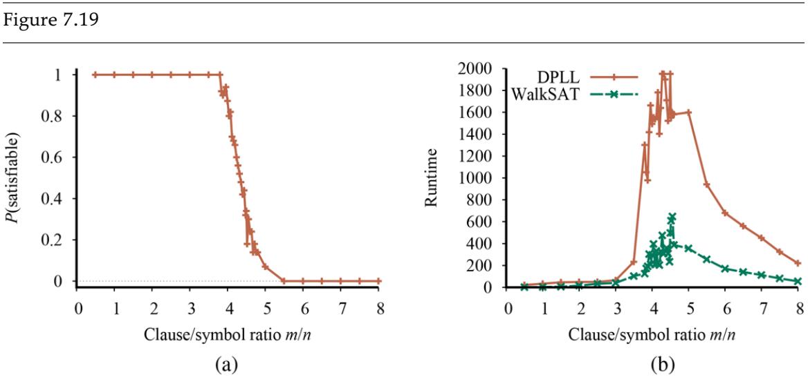
1. Graph showing the probability that a random 3-CNF sentence with symbols is satisfiable, as a function of the clause/symbol ratio . (b) Graph of the median run time (measured in number of iterations) for both DPLL and WALKSAT on random 3-CNF sentences. The most difficult problems have a clause/symbol ratio of about 4.3.

Theoretically, the satisfiability threshold conjecture says that for every , there is a threshold ratio such that, as goes to infinity, the probability that is

satisfiable becomes 1 for all values of below the threshold, and 0 for all values above. The conjecture remains unproven, even for special cases like . Whether it is a theorem or not, this kind of thresholding effect is certainly common, for satisfiability problems as well as other types of NP-hard problems.

Satisfiability threshold conjecture

Now that we have a good idea where the satisfiable and unsatisfiable problems are, the next question is, where are the hard problems? It turns out that they are also often at the threshold value. Figure 7.19(b) shows that 50-symbol problems at the threshold value of 4.3 are about 20 times more difficult to solve than those at a ratio of 3.3. The underconstrained problems are easiest to solve (because it is so easy to guess a solution); the overconstrained problems are not as easy as the underconstrained, but still are much easier than the ones right at the threshold.

7.7 Agents Based on Propositional Logic

In this section, we bring together what we have learned so far in order to construct wumpus world agents that use propositional logic. The first step is to enable the agent to deduce, to the extent possible, the state of the world given its percept history. This requires writing down a complete logical model of the effects of actions. We then show how logical inference can be used by an agent in the wumpus world. We also show how the agent can keep track of the world efficiently without going back into the percept history for each inference. Finally, we show how the agent can use logical inference to construct plans that are guaranteed to achieve its goals, provided its knowledge base is true in the actual world.

7.7.1 The current state of the world

As stated at the beginning of the chapter, a logical agent operates by deducing what to do from a knowledge base of sentences about the world. The knowledge base is composed of axioms—general knowledge about how the world works—and percept sentences obtained from the agent’s experience in a particular world. In this section, we focus on the problem of deducing the current state of the wumpus world—where am I, is that square safe, and so on.

We began collecting axioms in Section 7.4.3 . The agent knows that the starting square contains no pit ( ) and no wumpus ( ). Furthermore, for each square, it knows that the square is breezy if and only if a neighboring square has a pit; and a square is smelly if and only if a neighboring square has a wumpus. Thus, we include a large collection of sentences of the following form:

\[\begin{aligned} B\_{1,1} &\Leftrightarrow \left( P\_{1,2} \vee P\_{2,1} \right) \\ S\_{1,1} &\Leftrightarrow \left( W\_{1,2} \vee W\_{2,1} \right) \\ &\dots \end{aligned}\]

The agent also knows that there is exactly one wumpus. This is expressed in two parts. First, we have to say that there is at least one wumpus:

\[W\_{1,1} \lor W\_{1,2} \lor \cdots \lor W\_{4,3} \lor W\_{4,4} \text{ .}\]

Then we have to say that there is at most one wumpus. For each pair of locations, we add a sentence saying that at least one of them must be wumpus-free:

\[\begin{array}{c} \neg W\_{1,1} \lor \neg W\_{1,2} \\ \neg W\_{1,1} \lor \neg W\_{1,3} \\ \cdot \\ \neg W\_{4,3} \lor \neg W\_{4,4} \end{array}\]

So far, so good. Now let’s consider the agent’s percepts. We are using to mean there is a stench in [1,1]; can we use a single proposition, to mean that the agent perceives a stench? Unfortunately we can’t: if there was no stench at the previous time step, then would already be asserted, and the new assertion would simply result in a contradiction. The problem is solved when we realize that a percept asserts something only about the current time. Thus, if the time step (as supplied to MAKE-PERCEPT-SENTENCE in Figure 7.1 ) is 4, then we add to the knowledge base, rather than Strench—neatly avoiding any contradiction with . The same goes for the breeze, bump, glitter, and scream percepts.

The idea of associating propositions with time steps extends to any aspect of the world that changes over time. For example, the initial knowledge base includes —the agent is in square [1,1] at time 0—as well as , , and . We use the noun fluent (from the Latin fluens, flowing) to refer to an aspect of the world that changes. “Fluent” is a synonym for “state variable,” in the sense described in the discussion of factored representations in Section 2.4.7 on page 58. Symbols associated with permanent aspects of the world do not need a time superscript and are sometimes called atemporal variables.

Fluent

Atemporal variable

We can connect stench and breeze percepts directly to the properties of the squares where they are experienced as follows. For any time step and any square , we assert 11

11 Section 7.4.3 conveniently glossed over this requirement.

\[\begin{aligned} L\_{x,y}^t &\Rightarrow (Breez^t \Leftrightarrow B\_{x,y}) \\ L\_{x,y}^t &\Rightarrow (Stench^t \Leftrightarrow S\_{x,y}) \ . \end{aligned}\]

Fluent

Atemporal variable

Now, of course, we need axioms that allow the agent to keep track of fluents such as . These fluents change as the result of actions taken by the agent, so, in the terminology of Chapter 3 , we need to write down the transition model of the wumpus world as a set of logical sentences.

First we need proposition symbols for the occurrences of actions. As with percepts, these symbols are indexed by time; thus, means that the agent executes the Forward action at time 0. By convention, the percept for a given time step happens first, followed by the action for that time step, followed by a transition to the next time step.

To describe how the world changes, we can try writing effect axioms that specify the outcome of an action at the next time step. For example, if the agent is at location [1,1] facing east at time 0 and goes Forward, the result is that the agent is in square [2,1] and no longer is in :

(7.1)

Effect axiom

We would need one such sentence for each possible time step, for each of the 16 squares, and each of the four orientations. We would also need similar sentences for the other actions: Grab, Shoot, Climb, TurnLeft, and TurnRight.

Let us suppose that the agent does decide to move Forward at time 0 and asserts this fact into its knowledge base. Given the effect axiom in Equation (7.1) , combined with the initial assertions about the state at time 0, the agent can now deduce that it is in [2,1]. That is, . So far, so good. Unfortunately, if we , the answer is false, that is, the agent cannot prove it still has the arrow; nor can it prove it doesn’t have it! The information has been lost because the effect axiom fails to state what remains unchanged as the result of an action. The need to do this gives rise to the frame problem. One possible solution to the frame problem would be to add frame axioms explicitly asserting all the propositions that remain the same. For example, for each time we would have 12

12 The name “frame problem” comes from “frame of reference” in physics—the assumed stationary background with respect to which motion is measured. It also has an analogy to the frames of a movie, in which normally most of the background stays constant while changes occur in the foreground.

Frame problem

Frame axiom

where we explicitly mention every proposition that stays unchanged from time to time under the action Forward. Although the agent now knows that it still has the arrow after moving forward and that the wumpus hasn’t died or come back to life, the proliferation of frame axioms seems remarkably inefficient. In a world with different actions and

fluents, the set of frame axioms will be of size . This specific manifestation of the frame problem is sometimes called the representational frame problem. The problem played a significant role in the history of AI; we explore it further in the notes at the end of the chapter.

Representational frame problem

The representational frame problem is significant because the real world has very many fluents, to put it mildly. Fortunately for us humans, each action typically changes no more than some small number of those fluents—the world exhibits locality. Solving the representational frame problem requires defining the transition model with a set of axioms of size rather than size . There is also an inferential frame problem: the problem of projecting forward the results of a -step plan of action in time rather than .

Locality

Inferential frame problem

The solution to the problem involves changing one’s focus from writing axioms about actions to writing axioms about fluents. Thus for each fluent , we will have an axiom that defines the truth value of in terms of fluents (including itself) at time and the actions that may have occurred at time . Now, the truth value of can be set in one of two ways: either the action at time causes to be true at , or was already true at time and the action at time does not cause it to be false. An axiom of this form is called a successor-state axiom and has this form:

Successor-state axiom

One of the simplest successor-state axioms is the one for . Because there is no action for reloading, the part goes away and we are left with

\[HaveArray^{t+1} \Leftrightarrow \left(HaveArray^t \land \neg Shot^t\right). \tag{7.2}\]

For the agent’s location, the successor-state axioms are more elaborate. For example, is true if either (a) the agent moved Forward from [1,2] when facing south, or from [2,1] when facing west; or (b) was already true and the action did not cause movement (either because the action was not Forward or because the action bumped into a wall). Written out in propositional logic, this becomes

(7.3)

\[\begin{aligned} \left(L\_{1,1}^{t+1} &\Leftrightarrow \left(L\_{1,1}^t \land \left(\neg Forward^t \lor Bunp^{t+1}\right)\right)\right) \\ &\lor \left(L\_{1,2}^t \land \left(FacingSwath^t \land Formard^t\right)\right) \\ &\lor \left(L\_{2,1}^t \land \left(FacingWest^t \land Formard^t\right)\right). \end{aligned}\]

Exercise 7.SSAX asks you to write out axioms for the remaining wumpus world fluents.

Given a complete set of successor-state axioms and the other axioms listed at the beginning of this section, the agent will be able to ASK and answer any answerable question about the current state of the world. For example, in Section 7.2 the initial sequence of percepts and actions is

\[\begin{array}{l} \neg Stencil^{0} \wedge \neg Breze^{p} \wedge \neg Gitter^{0} \wedge \neg Bump^{0} \wedge \neg Screa^{m} \wedge \text{ } Formard^{0} \\ \neg Stention^{1} \wedge Breze^{p} \wedge \neg Gitter^{1} \wedge \neg Bump^{1} \wedge \neg Screa^{m} \wedge \neg TermRight^{1} \\ \neg Stention^{2} \wedge Breze^{2} \wedge \neg Gitter^{2} \wedge \neg Bump^{2} \wedge \neg Screa^{m} \wedge \neg TermRight^{2} \\ \neg Stention^{3} \wedge Breze^{3} \wedge \neg Gitter^{3} \wedge \neg Bump^{3} \wedge \neg Screa^{m} \wedge \neg Formard^{3} \\ \neg Stention^{4} \wedge \neg Breze^{4} \wedge \neg Gitter^{4} \wedge \neg Bump^{4} \wedge \neg Screa^{4} \wedge \neg TermRight^{4} \\ \neg Stention^{5} \wedge \neg Breze^{5} \wedge \neg Gitter^{5} \wedge \neg Bump^{5} \wedge \neg Scoream^{5} \wedge \neg Formal^{5} \\ \neg Stention^{6} \wedge \neg Bereze^{6} \wedge \neg Gitter^{6} \wedge \neg Bump^{6} \wedge \neg Screa^{m} \end{array}\]

At this point, we have , so the agent knows where it is. Moreover, and , so the agent has found the wumpus and one of the pits. The most important question for the agent is whether a square is OK to move into—that is, whether the square is free of a pit or live wumpus. It’s convenient to add axioms for this, having the form

\[OK\_{x,y}^t \Leftrightarrow \neg P\_{x,y} \land \neg (W\_{x,y} \land W cup plus t^t) \; .\]

Finally, ASK , so the square [2,2] is OK to move into. In fact, given a sound and complete inference algorithm such as DPLL, the agent can answer any answerable question about which squares are OK—and can do so in just a few milliseconds for small-tomedium wumpus worlds.

Solving the representational and inferential frame problems is a big step forward, but a pernicious problem remains: we need to confirm that all the necessary preconditions of an action hold for it to have its intended effect. We said that the Forward action moves the agent ahead unless there is a wall in the way, but there are many other unusual exceptions that could cause the action to fail: the agent might trip and fall, be stricken with a heart attack, be carried away by giant bats, etc. Specifying all these exceptions is called the qualification problem. There is no complete solution within logic; system designers have to use good judgment in deciding how detailed they want to be in specifying their model, and what details they want to leave out. We will see in Chapter 12 that probability theory allows us to summarize all the exceptions without explicitly naming them.

Qualification problem

7.7.2 A hybrid agent

The ability to deduce various aspects of the state of the world can be combined fairly straightforwardly with condition–action rules (see Section 2.4.2 ) and with problemsolving algorithms from Chapters 3 and 4 to produce a hybrid agent for the wumpus world. Figure 7.20 shows one possible way to do this. The agent program maintains and updates a knowledge base as well as a current plan. The initial knowledge base contains the atemporal axioms—those that don’t depend on , such as the axiom relating the breeziness of squares to the presence of pits. At each time step, the new percept sentence is added along with all the axioms that depend on , such as the successor-state axioms. (The next section explains why the agent doesn’t need axioms for future time steps.) Then, the agent uses logical inference, by ASKing questions of the knowledge base, to work out which squares are safe and which have yet to be visited.

Figure 7.20

A hybrid agent program for the wumpus world. It uses a propositional knowledge base to infer the state of the world, and a combination of problem-solving search and domain-specific code to choose actions. Each time HYBRID-WUMPUS-AGENT is called, it adds the percept to the knowledge base, and then either relies on a previously-defined plan or creates a new plan, and pops off the first step of the plan as the action to do next.

Hybrid agent

The main body of the agent program constructs a plan based on a decreasing priority of goals. First, if there is a glitter, the program constructs a plan to grab the gold, follow a route back to the initial location, and climb out of the cave. Otherwise, if there is no current plan, the program plans a route to the closest safe square that it has not visited yet, making sure the route goes through only safe squares.

Route planning is done with A* search, not with ASK. If there are no safe squares to explore, the next step—if the agent still has an arrow—is to try to make a safe square by shooting at one of the possible wumpus locations. These are determined by asking where is false—that is, where it is not known that there is not a wumpus. The function PLAN-SHOT (not shown) uses PLAN-ROUTE to plan a sequence of actions that will line up this shot. If this fails, the program looks for a square to explore that is not provably unsafe—that is, a square for which returns false. If there is no such square, then the mission is impossible and the agent retreats to [1,1] and climbs out of the cave.

7.7.3 Logical state estimation

The agent program in Figure 7.20 works quite well, but it has one major weakness: as time goes by, the computational expense involved in the calls to ASK goes up and up. This happens mainly because the required inferences have to go back further and further in time and involve more and more proposition symbols. Obviously, this is unsustainable—we cannot have an agent whose time to process each percept grows in proportion to the length of its life! What we really need is a constant update time—that is, independent of . The obvious answer is to save, or cache, the results of inference, so that the inference process at the next time step can build on the results of earlier steps instead of having to start again from scratch.

Caching

As we saw in Section 4.4 the history of percepts and all their ramifications can be replaced by the belief state—that is, some representation of the set of all possible current states of the world. The process of updating the belief state as new percepts arrive is called state estimation (see page 132). Whereas in Section 4.4 the belief state was an explicit list of states, here we can use a logical sentence involving the proposition symbols associated with the current time step, as well as the atemporal symbols. For example, the logical sentence 13

13 We can think of the percept history itself as a representation of the belief state, but one that makes inference increasingly expensive as the history gets longer.

\[WumpusAlive^1 \land L^1\_{2,1} \land B\_{2,1} \land \left(P\_{3,1} \lor P\_{2,2}\right) \tag{7.4}\]

represents the set of all states at time 1 in which the wumpus is alive, the agent is at [2,1], that square is breezy, and there is a pit in [3,1] or [2,2] or both.

Maintaining an exact belief state as a logical formula turns out not to be easy. If there are fluent symbols for time , then there are possible states—that is, assignments of truth values to those symbols. Now, the set of belief states is the powerset (set of all subsets) of the set of physical states. There are physical states, hence belief states. Even if we used the most compact possible encoding of logical formulas, with each belief state represented by a unique binary number, we would need numbers with bits to label the current belief state. That is, exact state estimation may require logical formulas whose size is exponential in the number of symbols.

One very common and natural scheme for approximate state estimation is to represent belief states as conjunctions of literals, that is, 1-CNF formulas. To do this, the agent program simply tries to prove and for each symbol (as well as each atemporal symbol whose truth value is not yet known), given the belief state at . The conjunction of provable literals becomes the new belief state, and the previous belief state is discarded.

It is important to understand that this scheme may lose some information as time goes along. For example, if the sentence in Equation (7.4) were the true belief state, then neither nor would be provable individually and neither would appear in the 1-CNF belief state. (Exercise 7.HYBR explores one possible solution to this problem.) On the other hand, because every literal in the 1-CNF belief state is proved from the previous belief state, and the initial belief state is a true assertion, we know that the entire 1-CNF belief state

must be true. Thus the set of possible states represented by the 1-CNF belief state includes all states that are in fact possible given the full percept history. As illustrated in Figure 7.21 , the 1-CNF belief state acts as a simple outer envelope, or conservative approximation, around the exact belief state. We see this idea of conservative approximations to complicated sets as a recurring theme in many areas of AI.

Figure 7.21

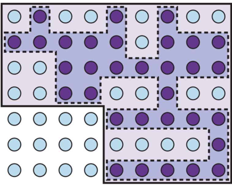
Depiction of a 1-CNF belief state (bold outline) as a simply representable, conservative approximation to the exact (wiggly) belief state (shaded region with dashed outline). Each possible world is shown as a circle; the shaded ones are consistent with all the percepts.

Conservative approximation

7.7.4 Making plans by propositional inference

The agent in Figure 7.20 uses logical inference to determine which squares are safe, but uses A* search to make plans. In this section, we show how to make plans by logical inference. The basic idea is very simple:

1. Construct a sentence that includes

• a. , a collection of assertions about the initial state;
• b. , the successor-state axioms for all possible actions at each time up to some maximum time ;
• c. the assertion that the goal is achieved at time :
• 2. Present the whole sentence to a SAT solver. If the solver finds a satisfying model, then the goal is achievable; if the sentence is unsatisfiable, then the problem is unsolvable.
• 3. Assuming a model is found, extract from the model those variables that represent actions and are assigned . Together they represent a plan to achieve the goals.

A propositional planning procedure, SATPLAN, is shown in Figure 7.22 . It implements the basic idea just given, with one twist. Because the agent does not know how many steps it will take to reach the goal, the algorithm tries each possible number of steps , up to some maximum conceivable plan length . In this way, it is guaranteed to find the shortest plan if one exists. Because of the way SATPLAN searches for a solution, this approach cannot be used in a partially observable environment; SATPLAN would just set the unobservable variables to the values it needs to create a solution.

Figure 7.22

The SATPLAN algorithm. The planning problem is translated into a CNF sentence in which the goal is asserted to hold at a fixed time step and axioms are included for each time step up to . If the satisfiability algorithm finds a model, then a plan is extracted by looking at those proposition symbols that refer to actions and are assigned true in the model. If no model exists, then the process is repeated with the goal moved one step later.

The key step in using SATPLAN is the construction of the knowledge base. It might seem, on casual inspection, that the wumpus world axioms in Section 7.7.1 suffice for steps 1(a) and 1(b) above. There is, however, a significant difference between the requirements for entailment (as tested by ASK) and those for satisfiability.

Consider, for example, the agent’s location, initially , and suppose the agent’s unambitious goal is to be in at time 1. The initial knowledge base contains and the goal is . Using ASK, we can prove if is asserted, and, reassuringly, we cannot prove if, say, is asserted instead. Now, SATPLAN will find the plan ; so far, so good.

Unfortunately, SATPLAN also finds the plan . How could this be? To find out, we inspect the model that SATPLAN constructs: it includes the assignment , that is, the agent can be in at time 1 by being there at time 0 and shooting. One might ask, “Didn’t we say the agent is in at time 0?” Yes, we did, but we didn’t tell the agent that it can’t be in two places at once! For entailment, is unknown and cannot, therefore, be used in a proof; for satisfiability, on the other hand, is unknown and can, therefore, be set to whatever value helps to make the goal true.

SATPLAN is a good debugging tool for knowledge bases because it reveals places where knowledge is missing. In this particular case, we can fix the knowledge base by asserting that, at each time step, the agent is in exactly one location, using a collection of sentences similar to those used to assert the existence of exactly one wumpus. Alternatively, we can assert for all locations other than ; the successor-state axiom for location takes care of subsequent time steps. The same fixes also work to make sure the agent has one and only one orientation at a time.

SATPLAN has more surprises in store, however. The first is that it finds models with impossible actions, such as shooting with no arrow. To understand why, we need to look more carefully at what the successor-state axioms (such as Equation (7.3) ) say about actions whose preconditions are not satisfied. The axioms do predict correctly that nothing will happen when such an action is executed (see Exercise 7.SATP), but they do not say that the action cannot be executed! To avoid generating plans with illegal actions, we must add precondition axioms Precondition axioms stating that an action occurrence requires the preconditions to be satisfied. , that 14

14 Notice that the addition of precondition axioms means that we need not include preconditions for actions in the successor-state axioms.

Precondition axioms

This ensures that if a plan selects the Shoot action at any time, it must be the case that the agent has an arrow at that time.

SATPLAN’s second surprise is the creation of plans with multiple simultaneous actions. For example, it may come up with a model in which both and are true, which is not allowed. To eliminate this problem, we introduce action exclusion axioms: for every pair of actions and we add the axiom

\[ \neg A\_i^t \lor \neg A\_j^t \dots \]

Action exclusion axiom

It might be pointed out that walking forward and shooting at the same time is not so hard to do, whereas, say, shooting and grabbing at the same time is rather impractical. By imposing action exclusion axioms only on pairs of actions that really do interfere with each other, we can allow for plans that include multiple simultaneous actions—and because SATPLAN finds the shortest legal plan, we can be sure that it will take advantage of this capability.

To summarize, SATPLAN finds models for a sentence containing the initial state, the goal, the successor-state axioms, the precondition axioms, and the action exclusion axioms. It can be shown that this collection of axioms is sufficient, in the sense that there are no longer any spurious “solutions.” Any model satisfying the propositional sentence will be a valid plan for the original problem. Modern SAT-solving technology makes the approach quite practical. For example, a DPLL-style solver has no difficulty in generating the solution for the wumpus world instance shown in Figure 7.2 .

This section has described a declarative approach to agent construction: the agent works by a combination of asserting sentences in the knowledge base and performing logical inference. This approach has some weaknesses hidden in phrases such as “for each time” and “for each square .” For any practical agent, these phrases have to be implemented by code that generates instances of the general sentence schema automatically for insertion into the knowledge base. For a wumpus world of reasonable size—one comparable to a smallish computer game—we might need a board and 1000 time steps, leading to knowledge bases with tens or hundreds of millions of sentences.

Not only does this become rather impractical, but it also illustrates a deeper problem: we know something about the wumpus world—namely, that the “physics” works the same way across all squares and all time steps—that we cannot express directly in the language of propositional logic. To solve this problem, we need a more expressive language, one in which phrases like “for each time” and “for each square” can be written in a natural way. First-order logic, described in Chapter 8 , is such a language; in first-order logic a wumpus world of any size and duration can be described in about ten logic sentences rather than ten million or ten trillion.

Summary

We have introduced knowledge-based agents and have shown how to define a logic with which such agents can reason about the world. The main points are as follows:

• Intelligent agents need knowledge about the world in order to reach good decisions.
• Knowledge is contained in agents in the form of sentences in a knowledge representation language that are stored in a knowledge base.
• A knowledge-based agent is composed of a knowledge base and an inference mechanism. It operates by storing sentences about the world in its knowledge base, using the inference mechanism to infer new sentences, and using these sentences to decide what action to take.
• A representation language is defined by its syntax, which specifies the structure of sentences, and its semantics, which defines the truth of each sentence in each possible world or model.
• The relationship of entailment between sentences is crucial to our understanding of reasoning. A sentence entails another sentence if is true in all worlds where is true. Equivalent definitions include the validity of the sentence and the unsatisfiability of the sentence .
• Inference is the process of deriving new sentences from old ones. Sound inference algorithms derive only sentences that are entailed; complete algorithms derive all sentences that are entailed.
• Propositional logic is a simple language consisting of proposition symbols and logical connectives. It can handle propositions that are known to be true, known to be false, or completely unknown.
• The set of possible models, given a fixed propositional vocabulary, is finite, so entailment can be checked by enumerating models. Efficient model-checking inference algorithms for propositional logic include backtracking and local search methods and can often solve large problems quickly.
• Inference rules are patterns of sound inference that can be used to find proofs. The resolution rule yields a complete inference algorithm for knowledge bases that are expressed in conjunctive normal form. Forward chaining and backward chaining are very natural reasoning algorithms for knowledge bases in Horn form.
• Local search methods such as WALKSAT can be used to find solutions. Such algorithms are sound but not complete.
• Logical state estimation involves maintaining a logical sentence that describes the set of possible states consistent with the observation history. Each update step requires inference using the transition model of the environment, which is built from successorstate axioms that specify how each fluent changes.
• Decisions within a logical agent can be made by SAT solving: finding possible models specifying future action sequences that reach the goal. This approach works only for fully observable or sensorless environments.
• Propositional logic does not scale to environments of unbounded size because it lacks the expressive power to deal concisely with time, space, and universal patterns of relationships among objects.

Bibliographical and Historical Notes

John McCarthy’s paper “Programs with Common Sense” (McCarthy, 1958, 1968) promulgated the notion of agents that use logical reasoning to mediate between percepts and actions. It also raised the flag of declarativism, pointing out that telling an agent what it needs to know is an elegant way to build software. Allen Newell’s (1982) article “The Knowledge Level” makes the case that rational agents can be described and analyzed at an abstract level defined by the knowledge they possess rather than the programs they run.

Logic itself had its origins in ancient Greek philosophy and mathematics. Plato discussed the syntactic structure of sentences, their truth and falsity, their meaning, and the validity of logical arguments. The first known systematic study of logic was Aristotle’s Organon. His syllogisms were what we now call inference rules, although they lacked the compositionality of our current rules.

Syllogism

The Megarian and Stoic schools began the systematic study of the basic logical connectives in the fifth century BCE. Truth tables are due to Philo of Megara. The Stoics took five basic inference rules as valid without proof, including the rule we now call Modus Ponens. They derived a number of other rules from these five, using, among other principles, the deduction theorem (page 222) and were clearer about proof than was Aristotle (Mates, 1953).

The idea of reducing logical inference to a purely mechanical process is due to Wilhelm Leibniz (1646–1716). George Boole (1847) introduced the first comprehensive and workable system of formal logic in his book The Mathematical Analysis of Logic. Boole’s logic was closely modeled on the ordinary algebra of real numbers and used substitution of logically equivalent expressions as its primary inference method. Although it didn’t handle all of propositional logic, other mathematicians soon filled in the missing pieces. Schröder (1877)

described conjunctive normal form, while Horn form was introduced much later by Alfred Horn (1951). The first comprehensive exposition of modern propositional logic (and firstorder logic) is found in Gottlob Frege’s (1879) Begriffschrift (“Concept Writing” or “Conceptual Notation”).

The first mechanical device to carry out logical inferences was the Stanhope Demonstrator, constructed by the third Earl of Stanhope (1753–1816). William Stanley Jevons, one of the mathematicians who extended Boole’s work, constructed his “logical piano” in 1869 to do inferences in Boolean logic. An entertaining history of these early mechanical inference devices is given by Martin Gardner (1968). The first computer programs for logical inference were Martin Davis’s 1954 program for proofs in Presburger arithmetic (Davis, 1957), and the Logic Theorist of Newell, Shaw, and Simon (1957).

Emil Post (1921) and Ludwig Wittgenstein (1922) independently used truth tables as a method of testing validity of propositional logic sentences. The Davis–Putnam algorithm (Davis and Putnam, 1960) was the first algorithm for propositional resolution, and the improved DPLL backtracking algorithm (Davis et al., 1962) proved to be more efficient. The resolution rule and a proof of its completeness were developed in full generality for firstorder logic by J. A. Robinson (1965).

Stephen Cook (1971) showed that deciding satisfiability of a sentence in propositional logic (the SAT problem) is NP-complete. Many subsets of propositional logic are known for which the satisfiability problem is polynomially solvable; Horn clauses are one such subset.

Early investigations showed that DPLL has polynomial average-case complexity for certain natural distributions of problems. Even better, Franco and Paull (1983) showed that the same problems could be solved in constant time simply by guessing random assignments. Motivated by the empirical success of local search, Koutsoupias and Papadimitriou (1992) showed that a simple hill-climbing algorithm can solve almost all satisfiability problem instances very quickly, suggesting that hard problems are rare. Schöning (1999) exhibited a randomized hill-climbing algorithm whose worst-case expected run time on 3-SAT problems is —still exponential, but substantially faster than previous worst-case bounds. The current record is (Rolf, 2006).

Efficiency gains in propositional solvers have been rapid. Given ten minutes of computing time, the original DPLL algorithm on 1962 hardware could solve only problems with 10 or 15 variables (on a 2019 laptop it would be about 30 variables). By 1995 the SATZ solver (Li and Anbulagan, 1997) could handle 1,000 variables, thanks to optimized data structures for indexing variables. Two crucial contributions were the watched literal indexing technique of Zhang and Stickel (1996), which makes unit propagation very efficient, and the introduction of clause (i.e., constraint) learning techniques from the CSP community by Bayardo and Schrag (1997). Using these ideas, and spurred by the prospect of solving industrial-scale circuit verification problems, Moskewicz et al. (2001) developed the CHAFF solver, which could handle problems with millions of variables. Beginning in 2002, annual SAT competitions have been held; most of the winning entries have been variants of CHAFF. The landscape of solvers is surveyed by Gomes et al. (2008).

Watched literal

Local search algorithms for satisfiability were tried by various authors throughout the 1980s, based on the idea of minimizing the number of unsatisfied clauses (Hansen and Jaumard, 1990). A particularly effective algorithm was developed by Gu (1989) and independently by Selman et al. (1992), who called it GSAT and showed that it was capable of solving a wide range of very hard problems very quickly. The WALKSAT algorithm described in this chapter is due to Selman et al. (1996).

The “phase transition” in satisfiability of random -SAT problems was first observed by Simon and Dubois (1989) and has given rise to a great deal of theoretical and empirical research—due, in part, to the connection to phase transition phenomena in statistical physics. Crawford and Auton (1993) located the 3-SAT transition at a clause/variable ratio of around 4.26, noting that this coincides with a sharp peak in the run time of their SAT solver. Cook and Mitchell (1997) provide an excellent summary of the early literature on the problem. Algorithms such as survey propagation (Parisi and Zecchina, 2002; Maneva et al., 2007) take advantage of special properties of random SAT instances near the satisfiability threshold and greatly outperform general SAT solvers on such instances. The current state of theoretical understanding is summarized by Achlioptas (2009).

Survey propagation

Good sources for information on satisfiability, both theoretical and practical, include the Handbook of Satisfiability (Biere et al., 2009), Donald Knuth’s (2015) fascicle on satisfiability, and the regular International Conferences on Theory and Applications of Satisfiability Testing, known as SAT.

The idea of building agents with propositional logic can be traced back to the seminal paper of McCulloch and Pitts (1943), which is well known for initiating the field of neural networks, but actually was concerned with the implementation of a Boolean circuit-based agent design in the brain. Stan Rosenschein (Rosenschein 1985; Kaelbling and Rosenschein, 1990) developed ways to compile circuit-based agents from declarative descriptions of the task environment. Rod Brooks (1986, 1989) demonstrates the effectiveness of circuit-based designs for controlling robots (see Chapter 26 ). Brooks (1991) argues that circuit-based designs are all that is needed for AI—that representation and reasoning are cumbersome, expensive, and unnecessary. In our view, both reasoning and circuits are necessary. Williams et al. (2003) describe a hybrid agent—not too different from our wumpus agent that controls NASA spacecraft, planning sequences of actions and diagnosing and recovering from faults.

The general problem of keeping track of a partially observable environment was introduced for state-based representations in Chapter 4 . Its instantiation for propositional representations was studied by Amir and Russell (2003), who identified several classes of environments that admit efficient state-estimation algorithms and showed that for several other classes the problem is intractable. The temporal-projection problem, which involves determining what propositions hold true after an action sequence is executed, can be seen as a special case of state estimation with empty percepts. Many authors have studied this problem because of its importance in planning; some important hardness results were established by Liberatore (1997). The idea of representing a belief state with propositions can be traced to Wittgenstein (1922).

Temporal-projection

The approach to logical state estimation using temporal indexes on propositional variables was proposed by Kautz and Selman (1992). Later generations of SATPLAN were able to take advantage of the advances in SAT solvers and remain among the most effective ways of solving difficult planning problems (Kautz, 2006).

The frame problem was first recognized by McCarthy and Hayes (1969). Many researchers considered the problem unsolvable within first-order logic, and it spurred a great deal of research into nonmonotonic logics. Philosophers from Dreyfus (1972) to Crockett (1994) have cited the frame problem as one symptom of the inevitable failure of the entire AI enterprise. The solution of the frame problem with successor-state axioms is due to Ray Reiter (1991). Thielscher (1999) identifies the inferential frame problem as a separate idea and provides a solution. In retrospect, one can see that Rosenschein’s (1985) agents were using circuits that implemented successor-state axioms, but Rosenschein did not notice that the frame problem was thereby largely solved.

Modern propositional solvers have been applied to a variety of industrial applications, such as the synthesis of computer hardware (Nowick et al., 1993). The SATMC satisfiability checker was used to detect a previously unknown vulnerability in a Web browser sign-on protocol (Armando et al., 2008).

The wumpus world was invented as a game by Gregory Yob (1975). Ironically, Yob developed it because he was bored with games played on a rectangular grid: he put his wumpus on a dodecahedron, and we put it back onto the boring old grid. Michael Genesereth suggested that the wumpus world be used as an agent testbed.

Chapter 8 First-Order Logic

In which we notice that the world is blessed with many objects, some of which are related to other objects, and in which we endeavor to reason about them.

Propositional logic sufficed to illustrate the basic concepts of logic, inference, and knowledge-based agents. Unfortunately, propositional logic is limited in what it can say. In this chapter, we examine first-order logic, which can concisely represent much more. We begin in Section 8.1 with a discussion of representation languages in general; Section 8.2 covers the syntax and semantics of first-order logic; Sections 8.3 and 8.4 illustrate the use of first-order logic for simple representations. 1

1 First-order logic is also called first-order predicate calculus; it may be abbreviated as FOL or FOPC.

First-order logic

8.1 Representation Revisited

In this section, we discuss the nature of representation languages. Programming languages (such as or Java or Python) are the largest class of formal languages in common use. Data structures within programs can be used to represent facts; for example, a program could use a array to represent the contents of the wumpus world. Thus, the programming language statement World[2,2] Pit is a fairly natural way to assert that there is a pit in square [2,2]. Putting together a string of such statements is sufficient for running a simulation of the wumpus world.

What programming languages lack is a general mechanism for deriving facts from other facts; each update to a data structure is done by a domain-specific procedure whose details are derived by the programmer from his or her own knowledge of the domain. This procedural approach can be contrasted with the declarative nature of propositional logic, in which knowledge and inference are separate, and inference is entirely domain independent. SQL databases take a mix of declarative and procedural knowledge.

A second drawback of data structures in programs (and of databases) is the lack of any easy way to say, for example, “There is a pit in [2,2] or [3,1]” or “If the wumpus is in [1,1] then he is not in [2,2].” Programs can store a single value for each variable, and some systems allow the value to be “unknown,” but they lack the expressiveness required to directly handle partial information.

Propositional logic is a declarative language because its semantics is based on a truth relation between sentences and possible worlds. It also has sufficient expressive power to deal with partial information, using disjunction and negation. Propositional logic has a third property that is desirable in representation languages, namely, compositionality. In a compositional language, the meaning of a sentence is a function of the meaning of its parts. For example, the meaning of ” ” is related to the meanings of ” ” and ” “. It would be very strange if” ” meant that there is a stench in square [1,4] and ” ” meant that there is a stench in square [1,2], but ” ” meant that France and Poland drew 1– 1 in last week’s ice hockey qualifying match.

However, propositional logic, as a factored representation, lacks the expressive power to concisely describe an environment with many objects. For example, we were forced to write a separate rule about breezes and pits for each square, such as

\[B\_{1,1} \Leftrightarrow \left(P\_{1,2} \vee P\_{2,1}\right).\]

In English, on the other hand, it seems easy enough to say, once and for all, “Squares adjacent to pits are breezy.” The syntax and semantics of English make it possible to describe the environment concisely: English, like first-order logic, is a structured representation.

8.1.1 The language of thought

Natural languages (such as English or Spanish) are very expressive indeed. We managed to write almost this whole book in natural language, with only occasional lapses into other languages (mainly mathematics and diagrams). There is a long tradition in linguistics and the philosophy of language that views natural language as a declarative knowledge representation language. If we could uncover the rules for natural language, we could use them in representation and reasoning systems and gain the benefit of the billions of pages that have been written in natural language.

The modern view of natural language is that it serves as a medium for communication rather than pure representation. When a speaker points and says, “Look!” the listener comes to know that, say, Superman has finally appeared over the rooftops. Yet we would not want to say that the sentence “Look!” represents that fact. Rather, the meaning of the sentence depends both on the sentence itself and on the context in which the sentence was spoken. Clearly, one could not store a sentence such as “Look!” in a knowledge base and expect to recover its meaning without also storing a representation of the context—which raises the question of how the context itself can be represented.

Natural languages also suffer from ambiguity, a problem for a representation language. As Pinker (1995) puts it: “When people think about spring, surely they are not confused as to

whether they are thinking about a season or something that goes boing—and if one word can correspond to two thoughts, thoughts can’t be words.”

The famous Sapir–Whorf hypothesis Whorf (1956) claims that our understanding of the world is strongly influenced by the language we speak. It is certainly true that different speech communities divide up the world differently. The French have two words “chaise” and “fauteuil,” for a concept that English speakers cover with one: “chair.” But English speakers can easily recognize the category fauteuil and give it a name—roughly “open-arm chair”—so does language really make a difference? Whorf relied mainly on intuition and speculation, and his ideas have been largely dismissed, but in the intervening years we actually have real data from anthropological, psychological, and neurological studies.

For example, can you remember which of the following two phrases formed the opening of Section 8.1 ?

“In this section, we discuss the nature of representation languages . . .”

“This section covers the topic of knowledge representation languages . . .”

Wanner (1974) did a similar experiment and found that subjects made the right choice at chance level—about 50% of the time—but remembered the content of what they read with better than 90% accuracy. This suggests that people interpret the words they read and form an internal nonverbal representation, and that the exact words are not consequential.

More interesting is the case in which a concept is completely absent in a language. Speakers of the Australian aboriginal language Guugu Yimithirr have no words for relative (or egocentric) directions, such as front, back, right, or left. Instead they use absolute directions, saying, for example, the equivalent of “I have a pain in my north arm.” This difference in language makes a difference in behavior: Guugu Yimithirr speakers are better at navigating in open terrain, while English speakers are better at placing the fork to the right of the plate.

Language also seems to influence thought through seemingly arbitrary grammatical features such as the gender of nouns. For example, “bridge” is masculine in Spanish and feminine in German. Boroditsky (2003) asked subjects to choose English adjectives to describe a

photograph of a particular bridge. Spanish speakers chose big, dangerous, strong, and towering, whereas German speakers chose beautiful, elegant, fragile, and slender.

Words can serve as anchor points that affect how we perceive the world. Loftus and Palmer (1974) showed experimental subjects a movie of an auto accident. Subjects who were asked “How fast were the cars going when they contacted each other?” reported an average of 32 mph, while subjects who were asked the question with the word “smashed” instead of “contacted” reported 41mph for the same cars in the same movie. Overall, there are measurable but small differences in cognitive processing by speakers of different languages, but no convincing evidence that this leads to a major difference in world view.

In a logical reasoning system that uses conjunctive normal form (CNF), we can see that the linguistic forms ” ” and ” ” are the same because we can look inside the system and see that the two sentences are stored as the same canonical CNF form. It is starting to become possible to do something similar with the human brain. Mitchell et al. (2008) put subjects in an functional magnetic resonance imaging (fMRI) machine, showed them words such as “celery,” and imaged their brains. A machine learning program trained on (word, image) pairs was able to predict correctly 77% of the time on binary choice tasks (e.g., “celery” or “airplane”). The system can even predict at above-chance levels for words it has never seen an fMRI image of before (by considering the images of related words) and for people it has never seen before (proving that fMRI reveals some level of common representation across people). This type of work is still in its infancy, but fMRI (and other imaging technology such as intracranial electrophysiology (Sahin et al., 2009)) promises to give us much more concrete ideas of what human knowledge representations are like.

From the viewpoint of formal logic, representing the same knowledge in two different ways makes absolutely no difference; the same facts will be derivable from either representation. In practice, however, one representation might require fewer steps to derive a conclusion, meaning that a reasoner with limited resources could get to the conclusion using one representation but not the other. For nondeductive tasks such as learning from experience, outcomes are necessarily dependent on the form of the representations used. We show in Chapter 19 that when a learning program considers two possible theories of the world, both of which are consistent with all the data, the most common way of breaking the tie is to choose the most succinct theory—and that depends on the language used to represent

theories. Thus, the influence of language on thought is unavoidable for any agent that does learning.

8.1.2 Combining the best of formal and natural languages

We can adopt the foundation of propositional logic—a declarative, compositional semantics that is context-independent and unambiguous—and build a more expressive logic on that foundation, borrowing representational ideas from natural language while avoiding its drawbacks. When we look at the syntax of natural language, the most obvious elements are nouns and noun phrases that refer to objects (squares, pits, wumpuses) and verbs and verb phrases along with adjectives and adverbs that refer to relations among objects (is breezy, is adjacent to, shoots). Some of these relations are functions—relations in which there is only one “value” for a given “input.” It is easy to start listing examples of objects, relations, and functions:

Object Relation Function

• Objects: people, houses, numbers, theories, Ronald McDonald, colors, baseball games, wars, centuries …
• Relations: these can be unary relations or properties such as red, round, bogus, prime, multistoried …, or more general -ary relations such as brother of, bigger than, inside, part of, has color, occurred after, owns, comes between, …

Property

Functions: father of, best friend, third inning of, one more than, beginning of …

Indeed, almost any assertion can be thought of as referring to objects and properties or relations. Some examples follow:

• “One plus two equals three.” Objects: one, two, three, one plus two; Relation: equals; Function: plus. (“One plus two” is a name for the object that is obtained by applying the function “plus” to the objects “one” and “two.” “Three” is another name for this object.)
• “Squares neighboring the wumpus are smelly.” Objects: wumpus, squares; Property: smelly; Relation: neighboring.
• “Evil King John ruled England in 1200.” Objects: John, England, 1200; Relation: ruled during; Properties: evil, king.

The language of first-order logic, whose syntax and semantics we define in the next section, is built around objects and relations. It has been important to mathematics, philosophy, and artificial intelligence precisely because those fields—and indeed, much of everyday human existence—can be usefully thought of as dealing with objects and the relations among them. First-order logic can also express facts about some or all of the objects in the universe. This enables one to represent general laws or rules, such as the statement “Squares neighboring the wumpus are smelly.”

The primary difference between propositional and first-order logic lies in the ontological commitment made by each language—that is, what it assumes about the nature of reality. Mathematically, this commitment is expressed through the nature of the formal models with respect to which the truth of sentences is defined. For example, propositional logic assumes that there are facts that either hold or do not hold in the world. Each fact can be in one of two states—true or false—and each model assigns true or false to each proposition symbol (see Section 7.4.2 ). First-order logic assumes more; namely, that the world consists of objects with certain relations among them that do or do not hold. (See Figure 8.1 .) The formal models are correspondingly more complicated than those for propositional logic.

Language	Ontological Commitment (What exists in the world)	Epistemological Commitment (What an agent believes about facts)
Propositional logic	facts	true/false/unknown
First-order logic	facts, objects, relations	true/false/unknown
Temporal logic	facts, objects, relations, times	true/false/unknown
Probability theory	facts	degree of belief ∈ 0, 1
Fuzzy logic	facts with degree of truth E 0, 1	known interval value

Formal languages and their ontological and epistemological commitments.

Ontological commitment

This ontological commitment is a great strength of logic (both propositional and first-order), because it allows us to start with true statements and infer other true statements. It is especially powerful in domains where every proposition has clear boundaries, such as mathematics or the wumpus world, where a square either does or doesn’t have a pit; there is no possibility of a square with a vaguely pit-like indentation. But in the real world, many propositions have vague boundaries: Is Vienna a large city? Does this restaurant serve delicious food? Is that person tall? It depends who you ask, and their answer might be “kind of.”

One response is to refine the representation: if a crude line dividing cities into “large” and “not large” leaves out too much information for the application in question, then one can increase the number of size categories or use a Population function symbol. Another proposed solution comes from Fuzzy logic, which makes the ontological commitment that propositions have a degree of truth between 0 and 1. For example, the sentence “Vienna is a large city” might be true to degree 0.8 in fuzzy logic, while “Paris is a large city” might be true to degree 0.9. This corresponds better to our intuitive conception of the world, but it makes it harder to do inference: instead of one rule to determine the truth of , fuzzy logic needs different rules depending on the domain. Another possibility, covered in Section 24.1 , is to assign each concept to a point in a multidimensional space, and then measure the distance between the concept “large city” and the concept “Vienna” or “Paris.”

Fuzzy logic

Degree of truth

Various special-purpose logics make still further ontological commitments; for example, temporal logic assumes that facts hold at particular times and that those times (which may be points or intervals) are ordered. Thus, special-purpose logics give certain kinds of objects (and the axioms about them) “first class” status within the logic, rather than simply defining them within the knowledge base. Higher-order logic views the relations and functions referred to by first-order logic as objects in themselves. This allows one to make assertions about all relations—for example, one could wish to define what it means for a relation to be transitive. Unlike most special-purpose logics, higher-order logic is strictly more expressive than first-order logic, in the sense that some sentences of higher-order logic cannot be expressed by any finite number of first-order logic sentences.

Temporal logic

Higher-order logic

A logic can also be characterized by its epistemological commitments—the possible states of knowledge that it allows with respect to each fact. In both propositional and first-order logic, a sentence represents a fact and the agent either believes the sentence to be true, believes it to be false, or has no opinion. These logics therefore have three possible states of knowledge regarding any sentence.

Epistemological commitment

Systems using probability theory, on the other hand, can have any degree of belief, or subjective likelihood, ranging from 0 (total disbelief) to 1 (total belief). It is important not to confuse the degree of belief in probability theory with the degree of truth in fuzzy logic. Indeed, some fuzzy systems allow uncertainty (degree of belief) about degrees of truth. For example, a probabilistic wumpus-world agent might believe that the wumpus is in [1,3] with probability 0.75 and in [2, 3] with probability 0.25 (although the wumpus is definitely in one particular square).

8.2 Syntax and Semantics of First-Order Logic

We begin this section by specifying more precisely the way in which the possible worlds of first-order logic reflect the ontological commitment to objects and relations. Then we introduce the various elements of the language, explaining their semantics as we go along. The main points are how the language facilitates concise representations and how its semantics leads to sound reasoning procedures.

8.2.1 Models for first-order logic

Chapter 7 said that the models of a logical language are the formal structures that constitute the possible worlds under consideration. Each model links the vocabulary of the logical sentences to elements of the possible world, so that the truth of any sentence can be determined. Thus, models for propositional logic link proposition symbols to predefined truth values.

Models for first-order logic are much more interesting. First, they have objects in them! The domain of a model is the set of objects or domain elements it contains. The domain is required to be nonempty—every possible world must contain at least one object. (See Exercise 8.EMPT for a discussion of empty worlds.) Mathematically speaking, it doesn’t matter what these objects are—all that matters is how many there are in each particular model—but for pedagogical purposes we’ll use a concrete example. Figure 8.2 shows a model with five objects: Richard the Lionheart, King of England from 1189 to 1199; his younger brother, the evil King John, who ruled from 1199 to 1215; the left legs of Richard and John; and a crown.

Figure 8.2

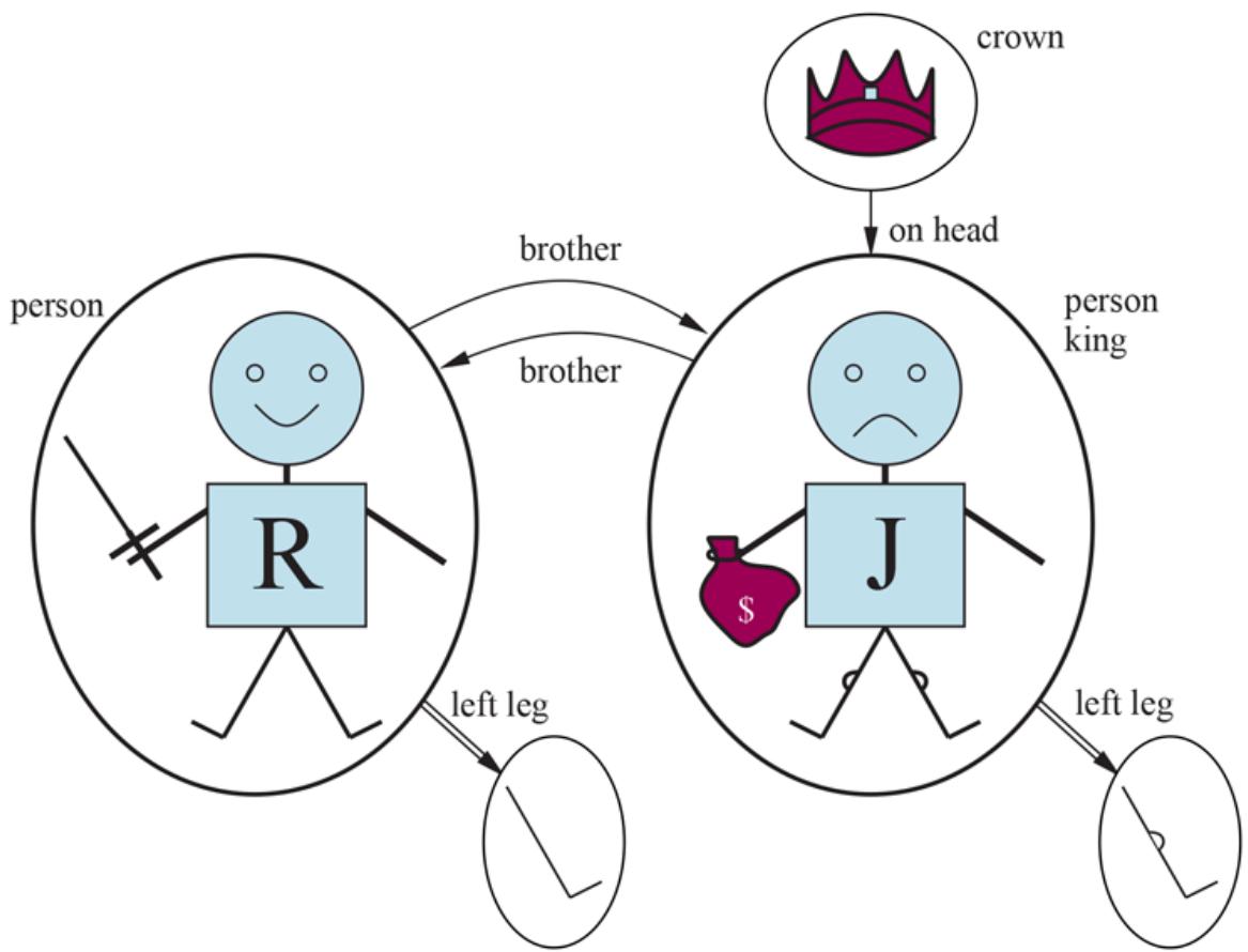
A model containing five objects, two binary relations (brother and on-head), three unary relations (person, king, and crown), and one unary function (left-leg).

Domain

Domain elements

The objects in the model may be related in various ways. In the figure, Richard and John are brothers. Formally speaking, a relation is just the set of tuples of objects that are related. (A tuple is a collection of objects arranged in a fixed order and is written with angle brackets surrounding the objects.) Thus, the brotherhood relation in this model is the set

Tuple

(Here we have named the objects in English, but you may, if you wish, mentally substitute the pictures for the names.) The crown is on King John’s head, so the “on head” relation contains just one tuple, 〈the crown, King John〉. The “brother” and “on head” relations are binary relations—that is, they relate pairs of objects. The model also contains unary relations, or properties: the “person” property is true of both Richard and John; the “king” property is true only of John (presumably because Richard is dead at this point); and the “crown” property is true only of the crown.

Certain kinds of relationships are best considered as functions, in that a given object must be related to exactly one object in this way. For example, each person has one left leg, so the model has a unary “left leg” function—a mapping from a one-element tuple to an object that includes the following mappings:

(8.2)

Strictly speaking, models in first-order logic require total functions, that is, there must be a value for every input tuple. Thus the crown must have a left leg and so must each of the left legs. There is a technical solution to this awkward problem involving an additional “invisible” object that is the left leg of everything that has no left leg, including itself. Fortunately, as long as one makes no assertions about the left legs of things that have no left legs, these technicalities are of no import.

Total functions

(8.1)

So far, we have described the elements that populate models for first-order logic. The other essential part of a model is the link between those elements and the vocabulary of the logical sentences, which we explain next.

8.2.2 Symbols and interpretations

We turn now to the syntax of first-order logic. The impatient reader can obtain a complete description from the formal grammar in Figure 8.3 .

Figure 8.3

	Sentence -> AtomicSentence ComplexSentence
	AtomicSentence -> Predicate Predicate(Term, ) Term = Term
ComplexSentence -> (Sentence)
	- Sentence
	Sentence A Sentence
	Sentence V Sentence
	Sentence => Sentence
	Sentence & Sentence
	Quantifier Variable, . Sentence
	Term -> Function(Term, .)
	Constant
	Variable
Quantifier ->	A
	Constant -> A X1 John
	Variable -> a x s ···
	Predicate -> True False After Loves Raining
	Function -> Mother LeftLeg
ERATOR PRECEDENCE : - - , =, ^, V, =>, <

The syntax of first-order logic with equality, specified in Backus–Naur form (see page 1030 if you are not familiar with this notation). Operator precedences are specified, from highest to lowest. The precedence of quantifiers is such that a quantifier holds over everything to the right of it.

The basic syntactic elements of first-order logic are the symbols that stand for objects, relations, and functions. The symbols, therefore, come in three kinds: constant symbols, which stand for objects; predicate symbols, which stand for relations; and function symbols, which stand for functions. We adopt the convention that these symbols will begin with uppercase letters. For example, we might use the constant symbols Richard and John; the predicate symbols Brother, OnHead, Person, King, and Crown; and the function symbol LeftLeg. As with proposition symbols, the choice of names is entirely up to the user. Each predicate and function symbol comes with an arity that fixes the number of arguments.

Constant symbol

Predicate symbol

Function symbol

Arity

Every model must provide the information required to determine if any given sentence is true or false. Thus, in addition to its objects, relations, and functions, each model includes an interpretation that specifies exactly which objects, relations and functions are referred to by the constant, predicate, and function symbols. One possible interpretation for our example—which a logician would call the intended interpretation—is as follows:

Interpretation

Intended interpretation

• Richard refers to Richard the Lionheart and John refers to the evil King John.
• Brother refers to the brotherhood relation—that is, the set of tuples of objects given in Equation (8.1) ; OnHead is a relation that holds between the crown and King John; Person, King, and Crown are unary relations that identify persons, kings, and crowns.
• LeftLeg refers to the “left leg” function as defined in Equation (8.2) .

There are many other possible interpretations, of course. For example, one interpretation maps Richard to the crown and John to King John’s left leg. There are five objects in the model, so there are 25 possible interpretations just for the constant symbols Richard and John. Notice that not all the objects need have a name—for example, the intended interpretation does not name the crown or the legs. It is also possible for an object to have several names; there is an interpretation under which both Richard and John refer to the crown. If you find this possibility confusing, remember that, in propositional logic, it is perfectly possible to have a model in which Cloudy and Sunny are both true; it is the job of the knowledge base to rule out models that are inconsistent with our knowledge. 2

2 Later, in Section 8.2.8 , we examine a semantics in which every object must have exactly one name.

In summary, a model in first-order logic consists of a set of objects and an interpretation that maps constant symbols to objects, function symbols to functions on those objects, and predicate symbols to relations. Just as with propositional logic, entailment, validity, and so on are defined in terms of all possible models. To get an idea of what the set of all possible models looks like, see Figure 8.4 . It shows that models vary in how many objects they contain—from one to infinity—and in the way the constant symbols map to objects.

Figure 8.4

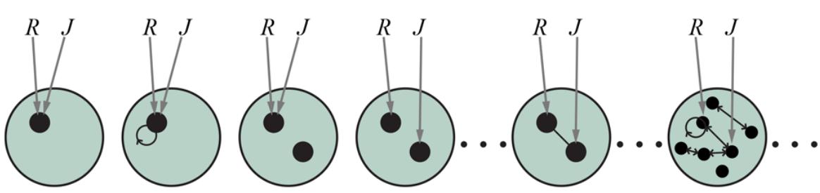
Some members of the set of all models for a language with two constant symbols, and , and one binary relation symbol. The interpretation of each constant symbol is shown by a gray arrow. Within each model, the related objects are connected by arrows.

Because the number of first-order models is unbounded, we cannot check entailment by enumerating them all (as we did for propositional logic). Even if the number of objects is restricted, the number of combinations can be very large. (See Exercise 8.MCNT.) For the example in Figure 8.4 , there are 137,506,194,466 models with six or fewer objects.

8.2.3 Terms

A term is a logical expression that refers to an object. Constant symbols are terms, but it is not always convenient to have a distinct symbol to name every object. In English we might use the expression “King John’s left leg” rather than giving a name to his leg. This is what function symbols are for: instead of using a constant symbol, we use LeftLeg(John). 3

3 -expressions (lambda expressions) provide a useful notation in which new function symbols are constructed “on the fly.” For example, the function that squares its argument can be written as and can be applied to arguments just like any other function symbol. A -expression can also be defined and used as a predicate symbol. The lambda operator in Lisp and Python plays exactly the same role. Notice that the use of in this way does not increase the formal expressive power of first-order logic, because any sentence that includes a expression can be rewritten by “plugging in” its arguments to yield an equivalent sentence.

Term

In the general case, a complex term is formed by a function symbol followed by a parenthesized list of terms as arguments to the function symbol. It is important to remember that a complex term is just a complicated kind of name. It is not a “subroutine call” that “returns a value.” There is no LeftLeg subroutine that takes a person as input and returns a leg. We can reason about left legs (e.g., stating the general rule that everyone has one and then deducing that John must have one) without ever providing a definition of LeftLeg. This is something that cannot be done with subroutines in programming languages.

The formal semantics of terms is straightforward. Consider a term . The function symbol refers to some function in the model (call it ); the argument terms refer to objects in the domain (call them ); and the term as a whole refers to the object that is the value of the function applied to . For example, suppose the LeftLeg function symbol refers to the function shown in Equation (8.2) and John refers to King John, then LeftLeg(John) refers to King John’s left leg. In this way, the interpretation fixes the referent of every term.

8.2.4 Atomic sentences

Now that we have terms for referring to objects and predicate symbols for referring to relations, we can combine them to make atomic sentences that state facts. An atomic sentence (or atom for short) is formed from a predicate symbol optionally followed by a parenthesized list of terms, such as

Atomic sentence

Atom

This states, under the intended interpretation given earlier, that Richard the Lionheart is the brother of King John. Atomic sentences can have complex terms as arguments. Thus, ⁴

4 We usually follow the argument-ordering convention that is read as ” is a of .”

states that Richard the Lionheart’s father is married to King John’s mother (again, under a suitable interpretation). 5

5 This ontology only recognizes one father and one mother for each person. A more complex ontology could recognize biological mother, birth mother, adoptive mother, etc.

An atomic sentence is true in a given model if the relation referred to by the predicate symbol holds among the objects referred to by the arguments.

8.2.5 Complex sentences

We can use logical connectives to construct more complex sentences, with the same syntax and semantics as in propositional calculus. Here are four sentences that are true in the model of Figure 8.2 under our intended interpretation:

8.2.6 Quantifiers

Once we have a logic that allows objects, it is only natural to want to express properties of entire collections of objects, instead of enumerating the objects by name. Quantifiers let us do this. First-order logic contains two standard quantifiers, called universal and existential.

Quantifier

Universal quantification (∀)

Recall the difficulty we had in Chapter 7 with the expression of general rules in propositional logic. Rules such as “Squares neighboring the wumpus are smelly” and “All kings are persons” are the bread and butter of first-order logic. We deal with the first of these in Section 8.3 . The second rule, “All kings are persons,” is written in first-order logic as

\[\forall x \,\,\,\,\,\underset{x}{\,\,\,} \,\,\,\underset{x}{\,\,\,} \,\,\, \_{Person}(x).\]

The universal quantifier is usually pronounced “For all”. (Remember that the upsidedown A stands for “all.”) Thus, the sentence says, “For all , if is a king, then is a person.” The symbol is called a variable. By convention, variables are lowercase letters. A variable is a term all by itself, and as such can also serve as the argument of a function—for example, . A term with no variables is called a ground term.

Universal quantifier

Variable

Ground term

Intuitively, the sentence , where is any logical sentence, says that is true for every object . More precisely, is true in a given model if is true in all possible extended interpretations constructed from the interpretation given in the model, where each extended interpretation specifies a domain element to which refers.

Extended interpretation

This sounds complicated, but it is really just a careful way of stating the intuitive meaning of universal quantification. Consider the model shown in Figure 8.2 and the intended interpretation that goes with it. We can extend the interpretation in five ways:

The universally quantified sentence is true in the original model if the sentence is true under each of the five extended interpretations. That is, the universally quantified sentence is equivalent to asserting the following five sentences:

Let us look carefully at this set of assertions. Since, in our model, King John is the only king, the second sentence asserts that he is a person, as we would hope. But what about the other four sentences, which appear to make claims about legs and crowns? Is that part of the meaning of “All kings are persons”? In fact, the other four assertions are true in the model, but make no claim whatsoever about the personhood qualifications of legs, crowns, or indeed Richard. This is because none of these objects is a king. Looking at the truth table for (Figure 7.8 on page 219), we see that the implication is true whenever its premise is false— regardless of the truth of the conclusion. Thus, by asserting the universally quantified sentence, which is equivalent to asserting a whole list of individual implications, we end up asserting the conclusion of the rule just for those objects for which the premise is true and saying nothing at all about those objects for which the premise is false. Thus, the truth-table definition of turns out to be perfect for writing general rules with universal quantifiers.

A common mistake, made frequently even by diligent readers who have read this paragraph several times, is to use conjunction instead of implication. The sentence

would be equivalent to asserting

and so on. Obviously, this does not capture what we want.

Existential quantification (∃)

Universal quantification makes statements about every object. Similarly, we can make a statement about some object without naming it, by using an existential quantifier. To say, for example, that King John has a crown on his head, we write

Existential quantifier

is pronounced “There exists an such that …” or “For some”.

Intuitively, the sentence says that is true for at least one object . More precisely, is true in a given model if is true in at least one extended interpretation that assigns to a domain element. That is, at least one of the following is true:

The fifth assertion is true in the model, so the original existentially quantified sentence is true in the model. Notice that, by our definition, the sentence would also be true in a model in which King John was wearing two crowns. This is entirely consistent with the original sentence “King John has a crown on his head.” 6

6 There is a variant of the existential quantifier, usually written or , that means “There exists exactly one.” The same meaning can be expressed using equality statements.

Just as appears to be the natural connective to use with is the natural connective to use with . Using as the main connective with led to an overly strong statement in the example in the previous section; using with usually leads to a very weak statement, indeed. Consider the following sentence:

On the surface, this might look like a reasonable rendition of our sentence. Applying the semantics, we see that the sentence says that at least one of the following assertions is true:

and so on. An implication is true if both premise and conclusion are true, or if its premise is false; so if Richard the Lionheart is not a crown, then the first assertion is true and the existential is satisfied. So, an existentially quantified implication sentence is true whenever any object fails to satisfy the premise; hence such sentences really do not say much at all.

Nested quantifiers

We will often want to express more complex sentences using multiple quantifiers. The simplest case is where the quantifiers are of the same type. For example, “Brothers are siblings” can be written as

Consecutive quantifiers of the same type can be written as one quantifier with several variables. For example, to say that siblinghood is a symmetric relationship, we can write

In other cases we will have mixtures. “Everybody loves somebody” means that for every person, there is someone that person loves:

\[ \forall x \; \exists \; y \; Loves(x, y) \; . \]

On the other hand, to say “There is someone who is loved by everyone,” we write

\[ \exists \, y \,\,\forall x \,\, Loves(x, y) \,\,. \]

The order of quantification is therefore very important. It becomes clearer if we insert parentheses. says that everyone has a particular property, namely, the property that they love someone. On the other hand, says that someone in the world has a particular property, namely the property of being loved by everybody.

Some confusion can arise when two quantifiers are used with the same variable name. Consider the sentence

\[\forall x \ (Crown(x) \lor (\exists x \ Bmother(Richard, x)))\ .\]

Here the in is existentially quantified. The rule is that the variable belongs to the innermost quantifier that mentions it; then it will not be subject to any other quantification. Another way to think of it is this: is a sentence about Richard (that he has a brother), not about ; so putting a outside it has no effect. It could equally well have been written . Because this can be a source of confusion, we will always use different variable names with nested quantifiers.

Connections between ∀ and ∃

The two quantifiers are actually intimately connected with each other, through negation. Asserting that everyone dislikes parsnips is the same as asserting there does not exist someone who likes them, and vice versa:

We can go one step further: “Everyone likes ice cream” means that there is no one who does not like ice cream:

Because is really a conjunction over the universe of objects and is a disjunction, it should not be surprising that they obey De Morgan’s rules. The De Morgan rules for quantified and unquantified sentences are as follows:

\[\begin{array}{ccccccccc}\neg\exists x & P&\equiv&\forall x&\neg P&\neg(P\lor Q)&\equiv&\neg P\land\neg Q\\\neg\forall x&\quad P&\equiv&\exists x&\neg P&\neg(P\land Q)&\equiv&\neg P\lor\neg Q\\\forall x&\quad P&\equiv&\neg\exists x&\quad\neg P&\quad P\land Q&\equiv&\neg(\neg P\land\neg Q)\\\exists x&\quad P&\equiv&\neg\forall x&\quad\neg P&\quad P\lor Q&\equiv&\neg(\neg P\land\neg Q).\end{array}\]

Thus, we do not really need both and , just as we do not really need both and . Still, readability is more important than parsimony, so we will keep both of the quantifiers.

8.2.7 Equality

First-order logic includes one more way to make atomic sentences, other than using a predicate and terms as described earlier. We can use the equality symbol to signify that two terms refer to the same object. For example,

\[Father(John) = Henry\]

Equality symbol

says that the object referred to by Father(John) and the object referred to by Henry are the same. Because an interpretation fixes the referent of any term, determining the truth of an equality sentence is simply a matter of seeing that the referents of the two terms are the same object.

The equality symbol can be used to state facts about a given function, as we just did for the Father symbol. It can also be used with negation to insist that two terms are not the same object. To say that Richard has at least two brothers, we would write

The sentence

does not have the intended meaning. In particular, it is true in the model of Figure 8.2 , where Richard has only one brother. To see this, consider the extended interpretation in which both and are assigned to King John. The addition of rules out such models. The notation is sometimes used as an abbreviation for .

8.2.8 Database semantics

Continuing the example from the previous section, suppose that we believe that Richard has two brothers, John and Geoffrey. We could write 7

7 Actually he had four, the others being William and Henry.

(8.3)

but that wouldn’t completely capture the state of affairs. First, this assertion is true in a model where Richard has only one brother—we need to add . Second, the sentence doesn’t rule out models in which Richard has many more brothers besides John and Geoffrey. Thus, the correct translation of “Richard’s brothers are John and Geoffrey” is as follows:

This logical sentence seems much more cumbersome than the corresponding English sentence. But if we fail to translate the English properly, our logical reasoning system will make mistakes. Can we devise a semantics that allows a more straightforward logical sentence?

One proposal that is very popular in database systems works as follows. First, we insist that every constant symbol refer to a distinct object—the unique-names assumption. Second, we assume that atomic sentences not known to be true are in fact false—the closed-world assumption. Finally, we invoke domain closure, meaning that each model contains no more domain elements than those named by the constant symbols.

Unique-names assumption

Closed-world assumption

Domain closure

Under the resulting semantics, Equation (8.3) does indeed state that Richard has exactly two brothers, John and Geoffrey. We call this database semantics to distinguish it from the standard semantics of first-order logic. Database semantics is also used in logic programming systems, as explained in Section 9.4.4 .

Database semantics

It is instructive to consider the set of all possible models under database semantics for the same case as shown in Figure 8.4 (page 259). Figure 8.5 shows some of the models, ranging from the model with no tuples satisfying the relation to the model with all tuples satisfying the relation. With two objects, there are four possible two-element tuples, so there are different subsets of tuples that can satisfy the relation. Thus, there are 16 possible models in all—a lot fewer than the infinitely many models for the standard first-order semantics. On the other hand, the database semantics requires definite knowledge of what the world contains.

Figure 8.5

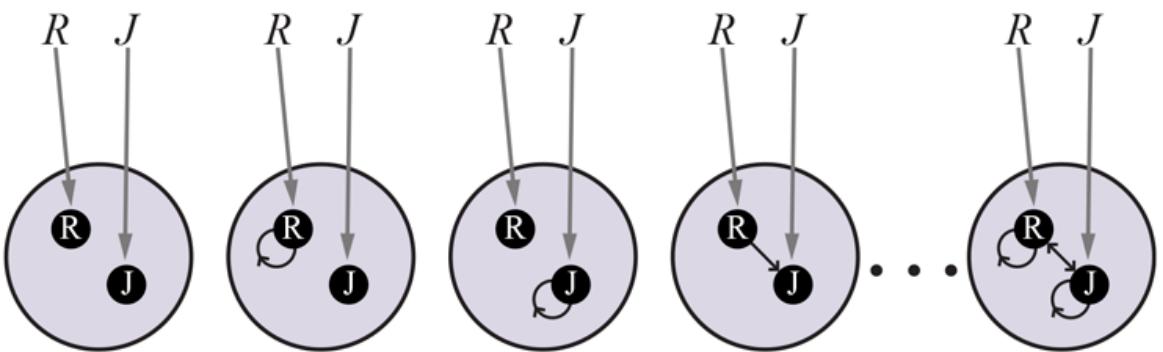
Some members of the set of all models for a language with two constant symbols, and , and one binary relation symbol, under database semantics. The interpretation of the constant symbols is fixed, and there is a distinct object for each constant symbol.

This example brings up an important point: there is no one “correct” semantics for logic. The usefulness of any proposed semantics depends on how concise and intuitive it makes the expression of the kinds of knowledge we want to write down, and on how easy and natural it is to develop the corresponding rules of inference. Database semantics is most useful when we are certain about the identity of all the objects described in the knowledge base and when we have all the facts at hand; in other cases, it is quite awkward. For the rest of this chapter, we assume the standard semantics while noting instances in which this choice leads to cumbersome expressions.

8.3 Using First-Order Logic

Now that we have defined an expressive logical language, let’s learn how to use it. In this section, we provide example sentences in some simple domains. In knowledge representation, a domain is just some part of the world about which we wish to express some knowledge.

Domain

We begin with a brief description of the TELL/ASK interface for first-order knowledge bases. Then we look at the domains of family relationships, numbers, sets, and lists, and at the wumpus world. Section 8.4.2 contains a more substantial example (electronic circuits) and Chapter 10 covers everything in the universe.

8.3.1 Assertions and queries in first-order logic

Sentences are added to a knowledge base using TELL, exactly as in propositional logic. Such sentences are called assertions. For example, we can assert that John is a king, Richard is a person, and all kings are persons:

Assertion

We can ask questions of the knowledge base using ASK. For example,

returns true. Questions asked with ASK are called queries or goals. Generally speaking, any query that is logically entailed by the knowledge base should be answered affirmatively. For example, given the three assertions above, the query

\[\text{Asx}(KB, Person(John))\]

should also return true. We can ask quantified queries, such as

\[\text{As\&} (KB, \; \exists x \; Person(x))\;.\]

The answer is true, but this is perhaps not as helpful as we would like. It is rather like answering “Can you tell me the time?” with “Yes.” If we want to know what value of makes the sentence true, we will need a different function, which we call ASKVARS,

\[\text{AsKVARS}(KB, Person(x))\]

and which yields a stream of answers. In this case there will be two answers: and . Such an answer is called a substitution or binding list. ASKVARS is usually reserved for knowledge bases consisting solely of Horn clauses, because in such knowledge bases every way of making the query true will bind the variables to specific values. That is not the case with first-order logic; in a that has been told only that there is no single binding to that makes the query true, even though the query is in fact true.

Substitution

Binding list

8.3.2 The kinship domain

The first example we consider is the domain of family relationships, or kinship. This domain includes facts such as “Elizabeth is the mother of Charles” and “Charles is the father of

William” and rules such as “One’s grandmother is the mother of one’s parent.”

Clearly, the objects in our domain are people. Unary predicates include Male and Female, among others. Kinship relations—parenthood, brotherhood, marriage, and so on—are represented by binary predicates: Parent, Sibling, Brother, Sister, Child, Daughter, Son, Spouse, Wife, Husband, Grandparent, Grandchild, Cousin, Aunt, and Uncle. We use functions for Mother and Father, because every person has exactly one of each of these, biologically (although we could introduce additional functions for adoptive mothers, surrogate mothers, etc.).

We can go through each function and predicate, writing down what we know in terms of the other symbols. For example, one’s mother is one’s parent who is female:

\[\forall m, c \; Mother(c) = m \LeftrightarrowFemale(m) \land Part(m, c) \; .\]

One’s husband is one’s male spouse:

\[\forall w, h \;\;Hausband(h, w) \Leftrightarrow \;Male(h) \land Spouse(h, w) \;.\]

Parent and child are inverse relations:

\[\forall p, c \; Pareto(p, c) \Leftrightarrowchild(c, p) \;.\]

A grandparent is a parent of one’s parent:

\[ \forall g, c \; Gradient(g, c) \Leftrightarrow \exists \; P \; Pareto(g, p) \land Pareto(p, c) \;. \]

A sibling is another child of one’s parent:

\[\forall x, y \; Sibling(x, y) \Leftrightarrow x \neq y \land \exists p \; Pareto(p, x) \land Partent(p, y) \;.\]

We could go on for several more pages like this, and Exercise 8.KINS asks you to do just that.

Each of these sentences can be viewed as an axiom of the kinship domain, as explained in Section 7.1 . Axioms are commonly associated with purely mathematical domains—we will see some axioms for numbers shortly—but they are needed in all domains. They provide the basic factual information from which useful conclusions can be derived. Our kinship axioms

are also definitions; they have the form . The axioms define the Mother function and the function and the Husband, Male, Parent, Grandparent, and Sibling predicates in terms of other predicates. Our definitions “bottom out” at a basic set of predicates (Child, Female, etc.) in terms of which the others are ultimately defined.

Definition

This is a natural way in which to build up the representation of a domain, and it is analogous to the way in which software packages are built up by successive definitions of subroutines from primitive library functions. Notice that there is not necessarily a unique set of primitive predicates; we could equally well have used Parent instead of Child. In some domains, as we show, there is no clearly identifiable basic set.

Not all logical sentences about a domain are axioms. Some are theorems—that is, they are entailed by the axioms. For example, consider the assertion that siblinghood is symmetric:

Theorem

Is this an axiom or a theorem? In fact, it is a theorem that follows logically from the axiom that defines siblinghood. If we ASK the knowledge base this sentence, it should return true.

From a purely logical point of view, a knowledge base need contain only axioms and no theorems, because the theorems do not increase the set of conclusions that follow from the knowledge base. From a practical point of view, theorems are essential to reduce the computational cost of deriving new sentences. Without them, a reasoning system has to start from first principles every time, rather like a physicist having to rederive the rules of calculus for every new problem.

Not all axioms are definitions. Some provide more general information about certain predicates without constituting a definition. Indeed, some predicates have no complete definition because we do not know enough to characterize them fully. For example, there is no obvious definitive way to complete the sentence

\[\forall x \; Person(x) \Leftrightarrow \dots\]

Fortunately, first-order logic allows us to make use of the Person predicate without completely defining it. Instead, we can write partial specifications of properties that every person has and properties that make something a person:

Axioms can also be “just plain facts,” such as Male(Jim) and Spouse(Jim,Laura). Such facts form the descriptions of specific problem instances, enabling specific questions to be answered. If all goes well, the answers to these questions will then be theorems that follow from the axioms.

Often, one finds that the expected answers are not forthcoming—for example, from Spouse(Jim,Laura) one expects (under the laws of many countries) to be able to infer that ; but this does not follow from the axioms given earlier—even after we add as suggested in Section 8.2.8 . This is a sign that an axiom is missing. Exercise 8.HILL asks the reader to supply it.

8.3.3 Numbers, sets, and lists

Numbers are perhaps the most vivid example of how a large theory can be built up from a tiny kernel of axioms. We describe here the theory of natural numbers or nonnegative integers. We need a predicate NatNum that will be true of natural numbers; we need one constant symbol, 0; and we need one function symbol, (successor). The Peano axioms define natural numbers and addition. Natural numbers are defined recursively: 8

⁸ The Peano axioms also include the principle of induction, which is a sentence of second-order logic rather than of first-order logic. The importance of this distinction is explained in Chapter 9 .

Natural numbers

Peano axioms

That is, 0 is a natural number, and for every object , if is a natural number, then is a natural number. So the natural numbers are , and so on. We also need axioms to constrain the successor function:

\[\begin{aligned} \forall n \ 0 \neq S(n). \\ \forall m, n \ m \neq n \Rightarrow S(m) \neq S(n). \end{aligned}\]

Now we can define addition in terms of the successor function:

\[\begin{aligned} \forall m \; NatNum(m) &\Rightarrow + (0, m) = m. \\ \forall m, n \; &\quad NatNum(m) \land NatNum(n) &\Rightarrow & + (S(m), n) = S(+(m, n)) \end{aligned}\]

The first of these axioms says that adding 0 to any natural number gives itself. Notice the use of the binary function symbol ” ” in the term ; in ordinary mathematics, the term would be written using infix notation. (The notation we have used for first-order logic is called prefix.) To make our sentences about numbers easier to read, we allow the use of infix notation. We can also write as , so the second axiom becomes

\[\forall m, n \; \begin{array}{c} \forall m \; \text{Nat} \newline Num(m) \land \text{Nat} \newline Num(n) \Rightarrow (m+1)+n = (m+n)+1 \; \end{array}\]

Infix

Prefix

This axiom reduces addition to repeated application of the successor function.

The use of infix notation is an example of syntactic sugar, that is, an extension to or abbreviation of the standard syntax that does not change the semantics. Any sentence that uses sugar can be “desugared” to produce an equivalent sentence in ordinary first-order logic. Another example is using square brackets rather than parentheses to make it easier to see what left bracket matches with what right bracket. Yet another example is collapsing quantifiers: replacing with .

Syntactic sugar

Once we have addition, it is straightforward to define multiplication as repeated addition, exponentiation as repeated multiplication, integer division and remainders, prime numbers, and so on. Thus, the whole of number theory (including cryptography) can be built up from one constant, one function, one predicate and four axioms.

The domain of sets is also fundamental to mathematics as well as to commonsense reasoning. (In fact, it is possible to define number theory in terms of set theory.) We want to be able to represent individual sets, including the empty set. We need a way to build up sets from elements or from operations on other sets. We will want to know whether an element is a member of a set and we will want to distinguish sets from objects that are not sets.

Set

We will use the normal vocabulary of set theory as syntactic sugar. The empty set is a constant written as . There is one unary predicate, Set, which is true of sets. The binary predicates are ( is a member of set ) and (set is a subset of , possibly equal to ). The binary functions are (intersection), (union), and (the set resulting from adding element to set ). One possible set of axioms is as follows: 1. The only sets are the empty set and those made by adding something to a set:

\[\forall s \; \; Set(s) \Leftrightarrow (s = \{\}) \lor (\exists x, s\_2 \qquad Set(s\_2) \land s = Add(x, s\_2)).\]

2. The empty set has no elements added into it. In other words, there is no way to decompose into a smaller set and an element:

\[ \neg \exists \, x, s \, \, Add(x, s) = \{\}. \]

3. Adding an element already in the set has no effect:

\[ \forall x, s \; x \in s \Leftrightarrow s = A dd(x, s) \; . \]

4. The only members of a set are the elements that were added into it. We express this recursively, saying that is a member of if and only if is equal to some element added to some set , where either is the same as or is a member of :

\[\forall x, s \; x \in s \iff \exists \; y, s\_2 \; (s = Add(y, s\_2) \land (x = y \lor x \in s\_2))\; .\]

5. A set is a subset of another set if and only if all of the first set’s members are members of the second set:

\[ \forall s\_1, s\_2 \; \; s\_1 \subseteq s\_2 \Leftrightarrow \left( \forall x \; \; x \in s\_1 \Rightarrow x \in s\_2 \right) \; . \]

6. Two sets are equal if and only if each is a subset of the other:

\[(\forall s\_1, s\_2 \; (s\_1 = s\_2) \Leftrightarrow (s\_1 \subseteq s\_2 \land s\_2 \subseteq s\_1) \; .)\]

7. An object is in the intersection of two sets if and only if it is a member of both sets:

\[ \forall x, s\_1, s\_2 \; x \in \left(s\_1 \cap s\_2\right) \Leftrightarrow \left(x \in s\_1 \land x \in s\_2\right). \]

8. An object is in the union of two sets if and only if it is a member of either set:

\[\forall x, s\_1, s\_2 \; x \in \left(s\_1 \cup s\_2\right) \Leftrightarrow \left(x \in s\_1 \lor x \in s\_2\right) \; .\]

Lists are similar to sets. The differences are that lists are ordered and the same element can List appear more than once in a list. We can use the vocabulary of Lisp for lists: Nil is the

constant list with no elements; Cons, Append, First, and Rest are functions; and Find is the predicate that does for lists what Member does for sets. List is a predicate that is true only of lists. As with sets, it is common to use syntactic sugar in logical sentences involving lists. The empty list is [ ]. The term Cons(x,Nil) (i.e., the list containing the element x followed by nothing) is written as [x]. A list of several elements, such as [A,B,C], corresponds to the nested term Cons(A,Cons(B,Cons(C,Nil))). Exercise 8.LIST asks you to write out the axioms for lists.

List

8.3.4 The wumpus world

Some propositional logic axioms for the wumpus world were given in Chapter 7 . The firstorder axioms in this section are much more concise, capturing in a natural way exactly what we want to say.

Recall that the wumpus agent receives a percept vector with five elements. The corresponding first-order sentence stored in the knowledge base must include both the percept and the time at which it occurred; otherwise, the agent will get confused about when it saw what. We use integers for time steps. A typical percept sentence would be

\[Percept([Stnch, Breeze,Glitter, None, None], 5) \dots\]

Here, Percept is a binary predicate, and Stench and so on are constants placed in a list. The actions in the wumpus world can be represented by logical terms:

To determine which is best, the agent program executes the query

\[\text{AskVARS}(KB, BestAction(a, 5)), \, 1\]

which returns a binding list such as . The agent program can then return as the action to take. The raw percept data implies certain facts about the current state. For

example:

4t,s,g,w,c Percept(s,Breeze,g,w,cl,t) => Breeze(t)
Ut,s,g,w,c Percept(s,None,g,w,c),t) => -Breeze(t)
4t,s,b,w,c Percept(s,b,Glitter,w,cl,t) => Glitter(t)
4t,s,b,w,c Percept(s,b,None,w,c],t) => -Glitter(t)

and so on. These rules exhibit a trivial form of the reasoning process called perception, which we study in depth in Chapter 25 . Notice the quantification over time . In propositional logic, we would need copies of each sentence for each time step.

Simple “reflex” behavior can also be implemented by quantified implication sentences. For example, we have

\[\forall t \; Gitter(t) \Rightarrow BestAction(Grab, t) \; .\]

Given the percept and rules from the preceding paragraphs, this would yield the desired conclusion —is the right thing to do.

We have represented the agent’s inputs and outputs; now it is time to represent the environment itself. Let us begin with objects. Obvious candidates are squares, pits, and the wumpus. We could name each square— and so on—but then the fact that and are adjacent would have to be an “extra” fact, and we would need one such fact for each pair of squares. It is better to use a complex term in which the row and column appear as integers; for example, we can simply use the list term . Adjacency of any two squares can be defined as

\[\forall x, y, a, b \; Adjacent([x, y], [a, b]) \Leftrightarrow (x = a \land (y = b - 1 \lor y = b + 1)) \lor (y = b \land (x = a - 1 \lor x = a + 1)).\]

We could name each pit, but this would be inappropriate for a different reason: there is no reason to distinguish among pits. It is simpler to use a unary predicate Pit that is true of squares containing pits. Finally, since there is exactly one wumpus, a constant Wumpus is just as good as a unary predicate (and perhaps more dignified from the wumpus’s viewpoint). 9

⁹ Similarly, most of us do not name each bird that flies overhead as it migrates to warmer regions in winter. An ornithologist wishing to study migration patterns, survival rates, and so on does name each bird, by means of a ring on its leg, because individual birds must be tracked.

The agent’s location changes over time, so we write to mean that the agent is at square at time . We can fix the wumpus to a specific location forever with . We can then say that objects can be at only one location at a time:

\[ \forall x, s\_1, s\_2, t \colon At(x, s\_1, t) \land At(x, s\_2, t) \Rightarrow s\_1 = s\_2 \; . \]

Given its current location, the agent can infer properties of the square from properties of its current percept. For example, if the agent is at a square and perceives a breeze, then that square is breezy:

\[ \forall s, t: At(Agent, s, t) \land Breezve(t) \Rightarrow Brezezy(s) \dots\]

It is useful to know that a square is breezy because we know that the pits cannot move about. Notice that Breezy has no time argument.

Having discovered which places are breezy (or smelly) and, very importantly, not breezy (or not smelly), the agent can deduce where the pits are (and where the wumpus is). Whereas propositional logic necessitates a separate axiom for each square (see and on page 220) and would need a different set of axioms for each geographical layout of the world, first-order logic just needs one axiom:

(8.4)

\[\forall s \; \; Breezy(s) \Leftrightarrow \exists \; r \; \; Adjacent(r, s) \land Pit(r) \; .\]

Similarly, in first-order logic we can quantify over time, so we need just one successor-state axiom for each predicate, rather than a different copy for each time step. For example, the axiom for the arrow (Equation (7.2) on page 240) becomes

\[\forall t \; \; HaveArray(t+1) \Leftrightarrow \left(HaveArray(t) \land \neg Action(Short, t)\right).\]

From these two example sentences, we can see that the first-order logic formulation is no less concise than the original English-language description given in Chapter 7 . The reader is invited to construct analogous axioms for the agent’s location and orientation; in these cases, the axioms quantify over both space and time. As in the case of propositional state estimation, an agent can use logical inference with axioms of this kind to keep track of

aspects of the world that are not directly observed. Chapter 11 goes into more depth on the subject of first-order successor-state axioms and their uses for constructing plans.

8.4 Knowledge Engineering in First-Order Logic

The preceding section illustrated the use of first-order logic to represent knowledge in three simple domains. This section describes the general process of knowledge-base construction —a process called knowledge engineering. A knowledge engineer is someone who investigates a particular domain, learns what concepts are important in that domain, and creates a formal representation of the objects and relations in the domain. We illustrate the knowledge engineering process in an electronic circuit domain. The approach we take is suitable for developing special-purpose knowledge bases whose domain is carefully circumscribed and whose range of queries is known in advance. General-purpose knowledge bases, which cover a broad range of human knowledge and are intended to support tasks such as natural language understanding, are discussed in Chapter 10 .

Knowledge engineering

8.4.1 The knowledge engineering process

Knowledge engineering projects vary widely in content, scope, and difficulty, but all such projects include the following steps:

• 1. IDENTIFY THE QUESTIONS. The knowledge engineer must delineate the range of questions that the knowledge base will support and the kinds of facts that will be available for each specific problem instance. For example, does the wumpus knowledge base need to be able to choose actions, or is it required only to answer questions about the contents of the environment? Will the sensor facts include the current location? The task will determine what knowledge must be represented in order to connect problem instances to answers. This step is analogous to the PEAS process for designing agents in Chapter 2 .
• 2. ASSEMBLE THE RELEVANT KNOWLEDGE. The knowledge engineer might already be an expert in the domain, or might need to work with real experts to extract what they know—a process called knowledge acquisition. At this stage, the

knowledge is not represented formally. The idea is to understand the scope of the knowledge base, as determined by the task, and to understand how the domain actually works.

Knowledge acquisition

For the wumpus world, which is defined by an artificial set of rules, the relevant knowledge is easy to identify. (Notice, however, that the definition of adjacency was not supplied explicitly in the wumpus-world rules.) For real domains, the issue of relevance can be quite difficult—for example, a system for simulating VLSI designs might or might not need to take into account stray capacitances and skin effects.

3. DECIDE ON A VOCABULARY OF PREDICATES, FUNCTIONS, AND

CONSTANTS. That is, translate the important domain-level concepts into logiclevel names. This involves many questions of knowledge-engineering style. Like programming style, this can have a significant impact on the eventual success of the project. For example, should pits be represented by objects or by a unary predicate on squares? Should the agent’s orientation be a function or a predicate? Should the wumpus’s location depend on time? Once the choices have been made, the result is a vocabulary that is known as the ontology of the domain. The word ontology means a particular theory of the nature of being or existence. The ontology determines what kinds of things exist, but does not determine their specific properties and interrelationships.

Ontology

4. ENCODE GENERAL KNOWLEDGE ABOUT THE DOMAIN. The knowledge engineer writes down the axioms for all the vocabulary terms. This pins down (to the extent possible) the meaning of the terms, enabling the expert to check the

content. Often, this step reveals misconceptions or gaps in the vocabulary that must be fixed by returning to step 3 and iterating through the process.

• 5. ENCODE A DESCRIPTION OF THE PROBLEM INSTANCE. If the ontology is well thought out, this step is easy. It involves writing simple atomic sentences about instances of concepts that are already part of the ontology. For a logical agent, problem instances are supplied by the sensors, whereas a “disembodied” knowledge base is given sentences in the same way that traditional programs are given input data.
• 6. POSE QUERIES TO THE INFERENCE PROCEDURE AND GET ANSWERS. This is where the reward is: we can let the inference procedure operate on the axioms and problem-specific facts to derive the facts we are interested in knowing. Thus, we avoid the need for writing an application-specific solution algorithm.
• 7. DEBUG AND EVALUATE THE KNOWLEDGE BASE. Alas, the answers to queries will seldom be correct on the first try. More precisely, the answers will be correct for the knowledge base as written, assuming that the inference procedure is sound, but they will not be the ones that the user is expecting. For example, if an axiom is missing, some queries will not be answerable from the knowledge base. A considerable debugging process could ensue. Missing axioms or axioms that are too weak can be easily identified by noticing places where the chain of reasoning stops unexpectedly. For example, if the knowledge base includes a diagnostic rule (see Exercise 8.WUMD) for finding the wumpus,

instead of the biconditional, then the agent will never be able to prove the absence of wumpuses. Incorrect axioms can be identified because they are false statements about the world. For example, the sentence

\[\forall x \; NumOfLegs(x, 4) \Rightarrow Mannmal(x)\]

is false for reptiles, amphibians, and tables. The falsehood of this sentence can be determined independently of the rest of the knowledge base. In contrast, a typical error in a program looks like this:

offset = position + 1.

It is impossible to tell whether offset should be position or position + 1 without understanding the surrounding context.

When you get to the point where there are no obvious errors in your knowledge base, it is tempting to declare success. But unless there are obviously no errors, it is better to formally evaluate your system by running it on a test suite of queries and measuring how many you get right. Without objective measurement, it is too easy to convince yourself that the job is done. To understand this seven-step process better, we now apply it to an extended example—the domain of electronic circuits.

8.4.2 The electronic circuits domain

We will develop an ontology and knowledge base that allow us to reason about digital circuits of the kind shown in Figure 8.6 . We follow the seven-step process for knowledge engineering.

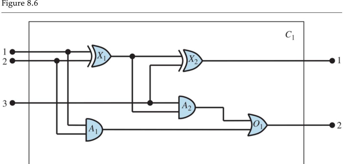
A digital circuit , purporting to be a one-bit full adder. The first two inputs are the two bits to be added, and the third input is a carry bit. The first output is the sum, and the second output is a carry bit for the next adder. The circuit contains two XOR gates, two AND gates, and one OR gate.

Identify the questions

There are many reasoning tasks associated with digital circuits. At the highest level, one analyzes the circuit’s functionality. For example, does the circuit in Figure 8.6 actually add properly? If all the inputs are high, what is the output of gate A2? Questions about the

circuit’s structure are also interesting. For example, what are all the gates connected to the first input terminal? Does the circuit contain feedback loops? These will be our tasks in this section. There are more detailed levels of analysis, including those related to timing delays, circuit area, power consumption, production cost, and so on. Each of these levels would require additional knowledge.

Assemble the relevant knowledge

What do we know about digital circuits? For our purposes, they are composed of wires and gates. Signals flow along wires to the input terminals of gates, and each gate produces a signal on the output terminal that flows along another wire. To determine what these signals will be, we need to know how the gates transform their input signals. There are four types of gates: AND, OR, and XOR gates have two input terminals, and NOT gates have one. All gates have one output terminal. Circuits, like gates, have input and output terminals.

To reason about functionality and connectivity, we do not need to talk about the wires themselves, the paths they take, or the junctions where they come together. All that matters is the connections between terminals—we can say that one output terminal is connected to another input terminal without having to say what actually connects them. Other factors such as the size, shape, color, or cost of the various components are irrelevant to our analysis.

If our purpose were something other than verifying designs at the gate level, the ontology would be different. For example, if we were interested in debugging faulty circuits, then it would probably be a good idea to include the wires in the ontology, because a faulty wire can corrupt the signal flowing along it. For resolving timing faults, we would need to include gate delays. If we were interested in designing a product that would be profitable, then the cost of the circuit and its speed relative to other products on the market would be important.

Decide on a vocabulary

We now know that we want to talk about circuits, terminals, signals, and gates. The next step is to choose functions, predicates, and constants to represent them. First, we need to be able to distinguish gates from each other and from other objects. Each gate is represented as an object named by a constant, about which we assert that it is a gate with, say, . The behavior of each gate is determined by its type: one of the constants AND,OR, XOR, or

NOT. Because a gate has exactly one type, a function is appropriate: . Circuits, like gates, are identified by a predicate: .

Next we consider terminals, which are identified by the predicate . A circuit can have one or more input terminals and one or more output terminals. We use the function to denote the first input terminal for circuit . A similar function is used for output terminals. The function says that circuit has input and output terminals. The connectivity between gates can be represented by a predicate, Connected, which takes two terminals as arguments, as in .

Finally, we need to know whether a signal is on or off. One possibility is to use a unary predicate, , which is true when the signal at a terminal is on. This makes it a little difficult, however, to pose questions such as “What are all the possible values of the signals at the output terminals of circuit ?” We therefore introduce as objects two signal values, 1 and 0, representing “on” and “off” respectively, and a function that denotes the signal value for the terminal .

Encode general knowledge of the domain

One sign that we have a good ontology is that we require only a few general rules, which can be stated clearly and concisely. These are all the axioms we will need:

1. If two terminals are connected, then they have the same signal:

\[\forall\_{t\_1, t\_2} Terminal(t\_1) \land Terminal(t\_2) \land Concented(t\_1, t\_2) \Rightarrow Signal(t\_1) = Signal(t\_2) \; .\]

2. The signal at every terminal is either 1 or 0:

\[\forall t \; Terminal(t) \Rightarrow Signal(t) = 1 \lor Signal(t) = 0.\]

3. Connected is commutative:

\[ \forall t\_1, t\_2 \; Connected(t\_1, t\_2) \Leftrightarrow Connected(t\_2, t\_1). \]

4. There are four types of gates:

\[\forall g \; Gate(g) \land k = Type(g) \Rightarrow k = AND \lor k = OR \lor k = XOR \lor k = NOT \dots\]

5. An AND gate’s output is 0 if and only if any of its inputs is 0:

\[\forall \, \_oGate(g) \land Type(g) = AND \Rightarrow Signal(Out(1, g)) = 0 \Leftrightarrow \exists n \, Signal(In(n, g)) = 0 \ . \, J\]

6. An OR gate’s output is 1 if and only if any of its inputs is 1:

\[\forall g \, Gate(g) \land Type(g) = OR \Rightarrow Signal(Out(1, g)) = 1 \Leftrightarrow \exists n \, Signal(In(n, g)) = 1 \; .\]

7. An XOR gate’s output is 1 if and only if its inputs are different:

\[\forall g \forall a \text{\(g\)} \land Type(g) = XOR \Rightarrow Signal(Out(1, g)) = 1 \Leftrightarrow Signal(In(n, g)) \neq Signal(In(2, g)) \dots\]

8. A NOT gate’s output is different from its input:

\[\forall\_q Gate(g) \land Type(g) = NOT \Rightarrow Signal(Out(1, g)) \neq Signal(In(1, g)).\]

9. The gates (except for NOT) have two inputs and one output.

\[\begin{aligned} \forall g &\quad &Gate(g) \land Type(g) = NOT & \Rightarrow & Array(g, 1, 1). \\ \forall g &\quad &Gate(g) \land k &= Type(g) \land (k = AND \lor k = OR \lor k = XOR) \Rightarrow Array(g, 2, 1). \end{aligned}\]

10. A circuit has terminals, up to its input and output arity, and nothing beyond its arity:

\[\begin{aligned} \forall c, i, j \; Circuit(c) \land Aarity(c, i, j) &\Rightarrow \\ \forall n \; (n \le i \Rightarrow Terminal \; (In \; (n, c))) \land (n > i \Rightarrow In \; (n, c) = Notling) \land \\ \forall n \; (n \le j \Rightarrow Terminal \; (In \; (n, c))) \land (n > j \Rightarrow Out \; (n, c) = Nothing) \end{aligned}\]

11. Gates, terminals, and signals are all distinct.

\[g \lor g, t, s \\ \text{Gate}(g) \land Terminal(t) \land Signal(s) \quad \Rightarrow \quad g \neq t \land g \neq s \land t \neq s.\]

12. Gates are circuits.

\[\forall g \; Gate(g) \Rightarrow Circuit(g)\]

Encode the specific problem instance

The circuit shown in Figure 8.6 is encoded as circuit with the following description. First we categorize the circuit and its component gates:

Then we show the connections between them:

Connected(Out(1,X1),In(1,X2))	Connected(In(1,C1),In(1,X1))
Connected(Out(1,X1),In(2,A2))	Connected(In(1,C1),In(1,A1))
Connected(Out(1,A2),In(1,O1))	Connected(In(2,C1),In(2,X1))
Connected(Out(1,A1),In(2,O1))	Connected(In(2,C1),In(2,A1))
Connected(Out(1,X2),Out(1,C1))	Connected(In(3,C1),In(2,X2))
Connected(Out(1,O1),Out(2,C1))	Connected(In(3,C1),In(1,A2)).

Pose queries to the inference procedure

What combinations of inputs would cause the first output of (the sum bit) to be 0 and the second output of (the carry bit) to be 1?

\[\begin{aligned} \exists \, i\_1, i\_2, i\_3 \; Signal(In(1, C\_1)) = i\_1 \land Signal(In(2, C\_1)) = i\_2 \land Signal(In(3, C\_1)) = i\_3 \\ \land Signal(Out(1, C\_1)) = 0 \land Signal(Out(2, C\_1)) = 1 \; \end{aligned}\]

The answers are substitutions for the variables , , and such that the resulting sentence is entailed by the knowledge base. ASKVARS will give us three such substitutions:

\[\{i\_1/1, i\_2/1, i\_3/0\} \quad \{i\_1/1, i\_2/0, i\_3/1\} \quad \{i\_1/0, i\_2/1, i\_3/1\}\]

What are the possible sets of values of all the terminals for the adder circuit?

\[\begin{aligned} \exists \, i\_1, i\_2, i\_3, o\_1, o\_2 \; Signal(In(1, C\_1)) = i\_1 \land Signal(In(2, C\_1)) = i\_2 \\ \land \; Signal(In(3, C\_1)) = i\_3 \land Signal(Out(1, C\_1)) = o\_1 \land Signal(Out(2, C\_1)) = o\_2 \end{aligned}\]

This final query will return a complete input–output table for the device, which can be used to check that it does in fact add its inputs correctly. This is a simple example of circuit verification. We can also use the definition of the circuit to build larger digital systems, for which the same kind of verification procedure can be carried out. (See Exercise 8.ADDR.) Many domains are amenable to the same kind of structured knowledge-base development, in which more complex concepts are defined on top of simpler concepts.

Debug the knowledge base

We can perturb the knowledge base in various ways to see what kinds of erroneous behaviors emerge. For example, suppose we fail to read Section 8.2.8 and hence forget to assert that . Suddenly, the system will be unable to prove any outputs for the circuit, except for the input cases 000 and 110. We can pinpoint the problem by asking for the outputs of each gate. For example, we can ask

\[i\_1 \exists i\_1, i\_2, o \; Signal(In(1, C\_1)) = i\_1 \land Signal(In(2, C\_1)) = i\_2 \land Signal(Out(1, X\_1)) = o, j\]

which reveals that no outputs are known at for the input cases 10 and 01. Then, we look at the axiom for XOR gates, as applied to :

\[Signal(Out(1, X\_1)) = 1 \Leftrightarrow Signal(In(1, X\_1)) \neq Signal(In(2, X\_1)) \ .\]

If the inputs are known to be, say, 1 and 0, then this reduces to

\[|Signal(Out(1, X\_1)) = 1 \Leftrightarrow 1 \neq 0 \ . \]

Now the problem is apparent: the system is unable to infer that , so we need to tell it that .

Summary

This chapter has introduced first-order logic, a representation language that is far more powerful than propositional logic. The important points are as follows:

• Knowledge representation languages should be declarative, compositional, expressive, context independent, and unambiguous.
• Logics differ in their ontological commitments and epistemological commitments. While propositional logic commits only to the existence of facts, first-order logic commits to the existence of objects and relations and thereby gains expressive power, appropriate for domains such as the wumpus world and electronic circuits.
• Both propositional logic and first-order logic share a difficulty in representing vague propositions. This difficulty limits their applicability in domains that require personal judgments, like politics or cuisine.
• The syntax of first-order logic builds on that of propositional logic. It adds terms to represent objects, and has universal and existential quantifiers to construct assertions about all or some of the possible values of the quantified variables.
• A possible world, or model, for first-order logic includes a set of objects and an interpretation that maps constant symbols to objects, predicate symbols to relations among objects, and function symbols to functions on objects.
• An atomic sentence is true only when the relation named by the predicate holds between the objects named by the terms. Extended interpretations, which map quantifier variables to objects in the model, define the truth of quantified sentences.
• Developing a knowledge base in first-order logic requires a careful process of analyzing the domain, choosing a vocabulary, and encoding the axioms required to support the desired inferences.

Bibliographical and Historical Notes

Although Aristotle’s logic dealt with generalizations over objects, it fell far short of the expressive power of first-order logic. A major barrier to its further development was its concentration on one-place predicates to the exclusion of many-place relational predicates. The first systematic treatment of relations was given by Augustus De Morgan (1864), who cited the following example to show the sorts of inferences that Aristotle’s logic could not handle: “All horses are animals; therefore, the head of a horse is the head of an animal.” This inference is inaccessible to Aristotle because any valid rule that can support this inference must first analyze the sentence using the two-place predicate ” is the head of .” The logic of relations was studied in depth by Charles Sanders Peirce (Peirce, 1870; Misak, 2004).

True first-order logic dates from the introduction of quantifiers in Gottlob Frege’s (1879) Begriffschrift (“Concept Writing” or “Conceptual Notation”). Peirce (1883) also developed first-order logic independently of Frege, although slightly later. Frege’s ability to nest quantifiers was a big step forward, but he used an awkward notation. The present notation for first-order logic is due substantially to Giuseppe Peano (1889), but the semantics is virtually identical to Frege’s. Oddly enough, Peano’s axioms were due in large measure to Grassmann (1861) and Dedekind (1888).

Leopold Löwenheim (1915) gave a systematic treatment of model theory for first-order logic, including the first proper treatment of the equality symbol. Löwenheim’s results were further extended by Thoralf Skolem (1920). Alfred Tarski (1935, 1956) gave an explicit definition of truth and model-theoretic satisfaction in first-order logic, using set theory.

John McCarthy (1958) was primarily responsible for the introduction of first-order logic as a tool for building AI systems. The prospects for logic-based AI were advanced significantly by Robinson’s (1965) development of resolution, a complete procedure for first-order inference. The logicist approach took root at Stanford University. Cordell Green, 1969a, 1969b developed a first-order reasoning system, QA3, leading to the first attempts to build a logical robot at SRI (Fikes and Nilsson, 1971). First-order logic was applied by Zohar Manna and Richard Waldinger (1971) for reasoning about programs and later by Michael Genesereth (1984) for reasoning about circuits. In Europe, logic programming (a restricted

form of first-order reasoning) was developed for linguistic analysis (Colmerauer et al., 1973) and for general declarative systems (Kowalski, 1974). Computational logic was also well entrenched at Edinburgh through the LCF (Logic for Computable Functions) project (Gordon et al., 1979). These developments are chronicled further in Chapters 9 and 10 .

Practical applications built with first-order logic include a system for evaluating the manufacturing requirements for electronic products (Mannion, 2002), a system for reasoning about policies for file access and digital rights management (Halpern and Weissman, 2008), and a system for the automated composition of Web services (McIlraith and Zeng, 2001).

Reactions to the Whorf hypothesis (Whorf, 1956) and the problem of language and thought in general, appear in multiple books (Pullum, 1991; Pinker, 2003) including the seemingly opposing titles Why the World Looks Different in Other Languages (Deutscher, 2010) and Why The World Looks the Same in Any Language (McWhorter, 2014) (although both authors agree that there are differences and the differences are small). The “theory” theory (Gopnik and Glymour, 2002; Tenenbaum et al., 2007) views children’s learning about the world as analogous to the construction of scientific theories. Just as the predictions of a machine learning algorithm depend strongly on the vocabulary supplied to it, so will the child’s formulation of theories depend on the linguistic environment in which learning occurs.

There are a number of good introductory texts on first-order logic, including some by leading figures in the history of logic: Alfred Tarski (1941), Alonzo Church (1956), and W.V. Quine (1982) (which is one of the most readable). Enderton (1972) gives a more mathematically oriented perspective. A highly formal treatment of first-order logic, along with many more advanced topics in logic, is provided by Bell and Machover (1977). Manna and Waldinger (1985) give a readable introduction to logic from a computer science perspective, as do Huth and Ryan (2004), who concentrate on program verification. Barwise and Etchemendy (2002) take an approach similar to the one used here. Smullyan (1995) presents results concisely, using the tableau format. Gallier (1986) provides an extremely rigorous mathematical exposition of first-order logic, along with a great deal of material on its use in automated reasoning. Logical Foundations of Artificial Intelligence (Genesereth and Nilsson, 1987) is both a solid introduction to logic and the first systematic treatment of logical agents with percepts and actions, and there are two good handbooks: van Bentham and ter Meulen (1997) and Robinson and Voronkov (2001). The journal of record for the

field of pure mathematical logic is the Journal of Symbolic Logic, whereas the Journal of Applied Logic deals with concerns closer to those of artificial intelligence.

Chapter 9 Inference in First-Order Logic

In which we define effective procedures for answering questions posed in first-order logic.

In this chapter, we describe algorithms that can answer any answerable first-order logic question. Section 9.1 introduces inference rules for quantifiers and shows how to reduce first-order inference to propositional inference, albeit at potentially great expense. Section 9.2 describes how unification can be used to construct inference rules that work directly with first-order sentences. We then discuss three major families of first-order inference algorithms: forward chaining (Section 9.3 ), backward chaining (Section 9.4 ), and resolution-based theorem proving (Section 9.5 ).

9.1 Propositional vs. First-Order Inference

One way to do first-order inference is to convert the first-order knowledge base to propositional logic and use propositional inference, which we already know how to do. A first step is eliminating universal quantifiers. For example, suppose our knowledge base contains the standard folkloric axiom that all greedy kings are evil:

From that we can infer any of the following sentences:

In general, the rule of Universal Instantiation (UI for short) says that we can infer any sentence obtained by substituting a ground term (a term without variables) for a universally quantified variable. 1

1 Do not confuse these substitutions with the extended interpretations used to define the semantics of quantifiers in Section 8.2.6 . The substitution replaces a variable with a term (a piece of syntax) to produce a new sentence, whereas an interpretation maps a variable to an object in the domain.

Universal Instantiation

To write out the inference rule formally, we use the notion of substitutions introduced in Section 8.3 . Let denote the result of applying the substitution to the sentence . Then the rule is written

for any variable and ground term . For example, the three sentences given earlier are obtained with the substitutions , , and .

Similarly, the rule of Existential Instantiation replaces an existentially quantified variable with a single new constant symbol. The formal statement is as follows: for any sentence , variable , and constant symbol that does not appear elsewhere in the knowledge base,

Existential Instantiation

For example, from the sentence

\[\exists x \; Crown(x) \land OnHead(x, John)\]

we can infer the sentence

as long as does not appear elsewhere in the knowledge base. Basically, the existential sentence says there is some object satisfying a condition, and applying the existential instantiation rule just gives a name to that object. Of course, that name must not already belong to another object. Mathematics provides a nice example: suppose we discover that there is a number that is a little bigger than 2.71828 and that satisfies the equation for . We can give this number the name , but it would be a mistake to give it the name of an existing object, such as . In logic, the new name is called a Skolem constant.

Skolem constant

Whereas Universal Instantiation can be applied many times to the same axiom to produce many different consequences, Existential Instantiation need only be applied once, and then the existentially quantified sentence can be discarded. For example, we no longer need once we have added the sentence .

9.1.1 Reduction to propositional inference

We now show how to convert any first-order knowledge base into a propositional knowledge base. The first idea is that, just as an existentially quantified sentence can be replaced by one instantiation, a universally quantified sentence can be replaced by the set of all possible instantiations. For example, suppose our knowledge base contains just the sentences

(9.1)

and that the only objects are and . We apply UI to the first sentence using all possible substitutions, and . We obtain

Next replace ground atomic sentences, such as , with proposition symbols, such as . Finally, apply any of the complete propositional algorithms in Chapter 7 to obtain conclusions such as , which is equivalent to .

This technique of propositionalization can be made completely general, as we show in Section 9.5 . However, there is a problem when the knowledge base includes a function symbol, the set of possible ground-term substitutions is infinite! For example, if the knowledge base mentions the symbol, then infinitely many nested terms such as can be constructed.

Propositionalization

Fortunately, there is a famous theorem due to Jacques Herbrand (1930) to the effect that if a sentence is entailed by the original, first-order knowledge base, then there is a proof involving just a finite subset of the propositionalized knowledge base. Since any such subset has a maximum depth of nesting among its ground terms, we can find the subset by first generating all the instantiations with constant symbols ( and ), then all terms of depth 1 ( and ), then all terms of depth 2, and so on, until we are able to construct a propositional proof of the entailed sentence.

We have sketched an approach to first-order inference via propositionalization that is complete—that is, any entailed sentence can be proved. This is a major achievement, given that the space of possible models is infinite. On the other hand, we do not know until the proof is done that the sentence is entailed! What happens when the sentence is not entailed? Can we tell? Well, for first-order logic, it turns out that we cannot. Our proof procedure can go on and on, generating more and more deeply nested terms, but we will not know whether it is stuck in a hopeless loop or whether the proof is just about to pop out. This is very much like the halting problem for Turing machines. Alan Turing (1936) and Alonzo Church (1936) both proved, in rather different ways, the inevitability of this state of affairs. The question of entailment for first-order logic is semidecidable—that is, algorithms exist that say yes to every entailed sentence, but no algorithm exists that also says no to every nonentailed sentence.

9.2 Unification and First-Order Inference

The sharp-eyed reader will have noticed that the propositionalization approach generates many unnecessary instantiations of universally quantified sentences. We’d rather have an approach that uses just the one rule, reasoning that solves the query as follows: given the rule that greedy kings are evil, find some such that is a king and is greedy, and then infer that this is evil. More generally, if there is some substitution that makes each of the conjuncts of the premise of the implication identical to sentences already in the knowledge base, then we can assert the conclusion of the implication, after applying . In this case, the substitution achieves that aim. Now suppose that instead of knowing , we know that everyone is greedy:

(9.2)

Then we would still like to be able to conclude that , because we know that John is a king (given) and John is greedy (because everyone is greedy). What we need for this to work is to find a substitution for both the variables in the implication sentence and the variables in the sentences that are in the knowledge base. In this case, applying the substitution to the implication premises and and the knowledge-base sentences and will make them identical. Thus, we can infer the consequent of the implication.

This inference process can be captured as a single inference rule that we call Generalized Modus Ponens: For atomic sentences , , and , where there is a substitution such that , for all , 2

\[\frac{(p\_1', \ p\_2', \ \dots, \ p\_n', \ (p\_1 \land p\_2 \land \dots \land p\_n \Rightarrow q)}{\text{SUBST}(\theta, q)} \cdot\]

2 Generalized Modus Ponens is more general than Modus Ponens (page 222) in the sense that the known facts and the premise of the

implication need match only up to a substitution, rather than exactly. On the other hand, Modus Ponens allows any sentence as the premise, rather than just a conjunction of atomic sentences.

Generalized Modus Ponens

There are premises to this rule: the atomic sentences and the one implication. The conclusion is the result of applying the substitution to the consequent . For our example:

p1’ is King(John)	p1 is King(x)
p2’ is Greedy(y)	p2 is Greedy(x)
0 is { x / John, y / John }	q is Evil(x)
SUBST(0,q) is Evil(John).

It is easy to show that Generalized Modus Ponens is a sound inference rule. First, we observe that, for any sentence (whose variables are assumed to be universally quantified) and for any substitution ,

\[p \vdash \text{Sussr}(\theta, p)\]

is true by Universal Instantiation. It is true in particular for a that satisfies the conditions of the Generalized Modus Ponens rule. Thus, from we can infer

\[\mathsf{Sussr}(\theta, p\_1') \land \dots \land \mathsf{Sussr}(\theta, p\_n')\]

and from the implication we can infer

\[\text{Substr}(\theta, p\_1) \land \dots \land \text{Substr}(\theta, p\_n) \Rightarrow \text{Substr}(\theta, q).\]

Now, in Generalized Modus Ponens is defined so that , for all ; therefore the first of these two sentences matches the premise of the second exactly. Hence, follows by Modus Ponens.

Generalized Modus Ponens is a lifted version of Modus Ponens—it raises Modus Ponens from ground (variable-free) propositional logic to first-order logic. We will see in the rest of this chapter that we can develop lifted versions of the forward chaining, backward chaining, and resolution algorithms introduced in Chapter 7 . The key advantage of lifted inference rules over propositionalization is that they make only those substitutions that are required to allow particular inferences to proceed.

Lifting

9.2.1 Unification

Lifted inference rules require finding substitutions that make different logical expressions look identical. This process is called unification and is a key component of all first-order inference algorithms. The UNIFY algorithm takes two sentences and returns a unifier for them (a substitution) if one exists:

Unification

Unifier

Let us look at some examples of how UNIFY should behave. Suppose we have a query : whom does John know? Answers to this query can be found by finding all sentences in the knowledge base that unify with . Here are the results of unification with four different sentences that might be in the knowledge base:

The last unification fails because cannot take on the values and at the same time. Now, remember that means “Everyone knows Elizabeth,” so we should be able to infer that John knows Elizabeth. The problem arises only because the two sentences happen to use the same variable name, . The problem can be avoided by standardizing apart one of the two sentences being unified, which means renaming its variables to avoid name clashes. For example, we can rename in to (a new variable name) without changing its meaning. Now the unification will work:

Standardizing apart

Exercise 9.STAN delves further into the need for standardizing apart.

There is one more complication: we said that UNIFY should return a substitution that makes the two arguments look the same. But there could be more than one such unifier. For example, could return or could return . The first unifier gives as the result of unification, whereas the second gives . The second result could be obtained from the first by an additional substitution ; we say that the first unifier is more general than the second, because it places fewer restrictions on the values of the variables.

Every unifiable pair of expressions has a single most general unifier (MGU) that is unique up to renaming and substitution of variables. For example, and are considered equivalent, as are and .

Most general unifier (MGU)

An algorithm for computing most general unifiers is shown in Figure 9.1 . The process is simple: recursively explore the two expressions simultaneously “side by side,” building up a unifier along the way, but failing if two corresponding points in the structures do not match. There is one expensive step: when matching a variable against a complex term, one must check whether the variable itself occurs inside the term; if it does, the match fails because no consistent unifier can be constructed. For example, can’t unify with . This socalled occur check makes the complexity of the entire algorithm quadratic in the size of the expressions being unified. Some systems, including many logic programming systems, simply omit the occur check and put the onus on the user to avoid making unsound inferences as a result. Other systems use more complex unification algorithms with lineartime complexity.

Figure 9.1

The unification algorithm. The arguments and can be any expression: a constant or variable, or a compound expression such as a complex sentence or term, or a list of expressions. The argument is a substitution, initially the empty substitution, but with pairs added to it as we recurse through the inputs, comparing the expressions element by element. In a compound expression such as , OP( ) field picks out the function symbol and ARGS( ) field picks out the argument list .

9.2.2 Storage and retrieval

Underlying the TELL, ASK, and ASKVARS functions used to inform and interrogate a knowledge base are the more primitive STORE and FETCH functions. STORE( ) stores a sentence into the knowledge base and FETCH( ) returns all unifiers such that the query unifies with some sentence in the knowledge base. The problem we used to illustrate unification—finding all facts that unify with —is an instance of FETCHing.

The simplest way to implement STORE and FETCH is to keep all the facts in one long list and unify each query against every element of the list. Such a process is inefficient, but it works. The remainder of this section outlines ways to make retrieval more efficient.

We can make FETCH more efficient by ensuring that unifications are attempted only with sentences that have some chance of unifying. For example, there is no point in trying to unify with . We can avoid such unifications by indexing the facts in the knowledge base. A simple scheme called predicate indexing puts all the facts in one bucket and all the facts in another. The buckets can be stored in a hash table for efficient access.

Indexing

Predicate indexing

Predicate indexing is useful when there are many predicate symbols but only a few clauses for each symbol. Sometimes, however, a predicate has many clauses. For example, suppose that the tax authorities want to keep track of who employs whom, using a predicate . This would be a very large bucket with perhaps millions of employers and

tens of millions of employees. Answering a query such as with predicate indexing would require scanning the entire bucket.

For this particular query, it would help if facts were indexed both by predicate and by second argument, perhaps using a combined hash table key. Then we could simply construct the key from the query and retrieve exactly those facts that unify with the query. For other queries, such as , we would need to have indexed the facts by combining the predicate with the first argument. Therefore, facts can be stored under multiple index keys, rendering them instantly accessible to various queries that they might unify with.

Given a sentence to be stored, it is possible to construct indices for all possible queries that unify with it. For the fact , the queries are

	Employs(IBM,Richard) Does IBM employ Richard?
Employs(x,Richard)	Who employs Richard?
Employs(IBM,y)	Whom does IBM employ?
Employs(x,y)	Who employs whom?

These queries form a subsumption lattice, as shown in Figure 9.2(a) . The lattice has some interesting properties. The child of any node in the lattice is obtained from its parent by a single substitution; and the “highest” common descendant of any two nodes is the result of applying their most general unifier. A sentence with repeated constants has a slightly different lattice, as shown in Figure 9.2(b) . Although function symbols are not shown in the figure, they too can be incorporated into the lattice structure.

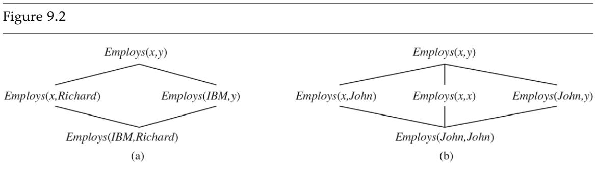
1. The subsumption lattice whose lowest node is . (b) The subsumption lattice for the sentence .

Subsumption lattice

For predicates with a small number of arguments, it is a good tradeoff to create an index for every point in the subsumption lattice. That requires a little more work at storage time, but speeds up retrieval time. However, for a predicate with arguments, the lattice contains nodes. If function symbols are allowed, the number of nodes is also exponential in the size of the terms in the sentence to be stored. This can lead to a huge number of indices.

We have to somehow limit the indices to ones that are likely to be used frequently in queries; otherwise we will waste more time in creating the indices than we save by having them. We could adopt a fixed policy, such as maintaining indices only on keys composed of a predicate plus a single argument. Or we could learn an adaptive policy that creates indices to meet the demands of the kinds of queries being asked. For commercial databases where facts number in the billions, the problem has been the subject of intensive study, technology development, and continual optimization.

9.3 Forward Chaining

In Section 7.5 we showed a forward-chaining algorithm for knowledge bases of propositional definite clauses. Here we expand that idea to cover first-order definite clauses.

Of course there are some logical sentences that cannot be stated as a definite clause, and thus cannot be handled by this approach. But rules of the form are sufficient to cover a wide variety of interesting real-world systems.

9.3.1 First-order definite clauses

First-order definite clauses are disjunctions of literals of which exactly one is positive. That means a definite clause is either atomic, or is an implication whose antecedent is a conjunction of positive literals and whose consequent is a single positive literal. Existential quantifiers are not allowed, and universal quantifiers are left implicit: if you see an in a definite clause, that means there is an implicit quantifier. A typical first-order definite clause looks like this:

but the literals and also count as definite clauses. First-order literals can include variables, so Greedy(y) is interpreted as “everyone is greedy” (the universal quantifier is implicit).

Let us put definite clauses to work in representing the following problem:

The law says that it is a crime for an American to sell weapons to hostile nations. The country Nono, an enemy of America, has some missiles, and all of its missiles were sold to it by Colonel West, who is American.

First, we will represent these facts as first-order definite clauses:

” it is a crime for an American to sell weapons to hostile nations”:

“Nono has some missiles.” The sentence is transformed into two definite clauses by Existential Instantiation, introducing a new constant :

(9.4)

\[Owns(Nono, M\_1)\]

(9.5)

“All of its missiles were sold to it by Colonel West”:

(9.6)

We will also need to know that missiles are weapons:

(9.7)

\[Missile(x) \Rightarrow Weapon(x).\]

and we must know that an enemy of America counts as “hostile”:

(9.8)

“West, who is American”:

(9.9)

“The country Nono, an enemy of America”:

This knowledge base happens to be a Datalog knowledge base: Datalog is a language consisting of first-order definite clauses with no function symbols. Datalog gets its name because it can represent the type of statements typically made in relational databases. The absence of function symbols makes inference much easier.

Datalog

9.3.2 A simple forward-chaining algorithm

Figure 9.3 shows a simple forward chaining inference algorithm. Starting from the known facts, it triggers all the rules whose premises are satisfied, adding their conclusions to the known facts. The process repeats until the query is answered (assuming that just one answer is required) or no new facts are added. Notice that a fact is not “new” if it is just a renaming of a known fact—a sentence is a renaming of another if they are identical except for the names of the variables. For example, and are renamings of each other. They both mean the same thing: “Everyone likes ice cream.”

Figure 9.3

A conceptually straightforward, but inefficient, forward-chaining algorithm. On each iteration, it adds to KB all the atomic sentences that can be inferred in one step from the implication sentences and the atomic sentences already in KB. The function STANDARDIZE-VARIABLES replaces all variables in its arguments with new ones that have not been used before.

Renaming

We use our crime problem to illustrate FOL-FC-ASK. The implication sentences available for chaining are (9.3), (9.6), (9.7), and (9.8). Two iterations are required:

• On the first iteration, rule (9.3) has unsatisfied premises. Rule (9.6) is satisfied with , and is added. Rule (9.7) is satisfied with , and is added. Rule (9.8) is satisfied with , and is added.
• On the second iteration, rule (9.3) is satisfied with , and the inference is added.

Figure 9.4 shows the proof tree that is generated. Notice that no new inferences are possible at this point because every sentence that could be concluded by forward chaining is already contained explicitly in the KB. Such a knowledge base is called a fixed point of the inference process. Fixed points reached by forward chaining with first-order definite clauses are similar to those for propositional forward chaining (page 231); the principal difference is that a first-order fixed point can include universally quantified atomic sentences.

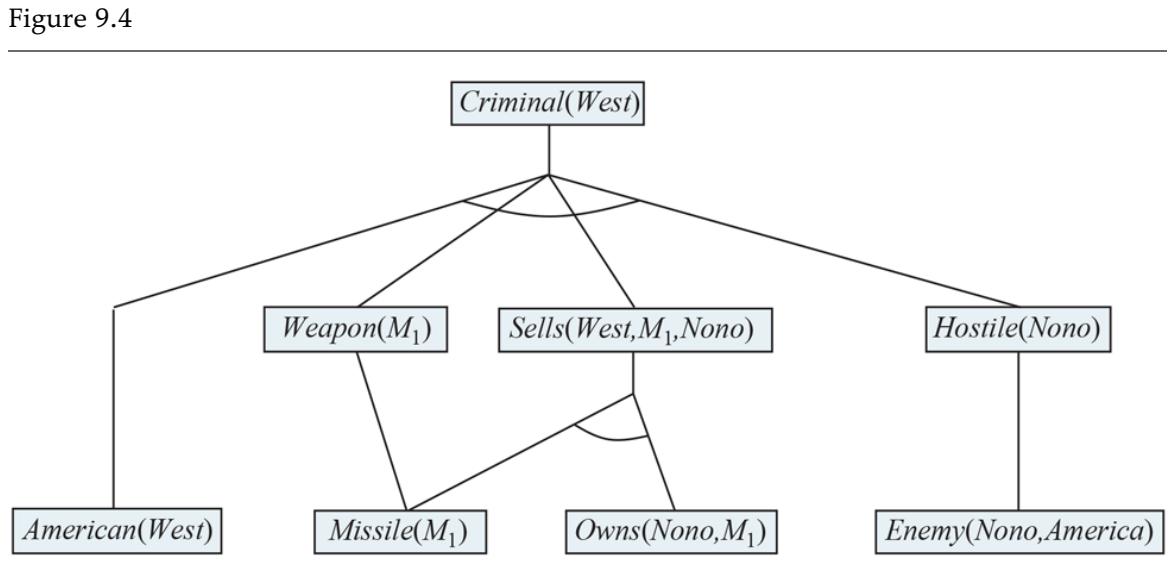
The proof tree generated by forward chaining on the crime example. The initial facts appear at the bottom level, facts inferred on the first iteration in the middle level, and facts inferred on the second iteration at the top level.

FOL-FC-ASK is easy to analyze. First, it is sound, because every inference is just an application of Generalized Modus Ponens, which is sound. Second, it is complete for definite clause knowledge bases; that is, it answers every query whose answers are entailed by any knowledge base of definite clauses.

For Datalog knowledge bases, which contain no function symbols, the proof of completeness is fairly easy. We begin by counting the number of possible facts that can be added, which determines the maximum number of iterations. Let be the maximum arity (number of arguments) of any predicate, be the number of predicates, and be the number of constant symbols. Clearly, there can be no more than distinct ground facts, so after this many iterations the algorithm must have reached a fixed point. Then we can make an argument very similar to the proof of completeness for propositional forward chaining. (See page 231.) The details of how to make the transition from propositional to first-order completeness are given for the resolution algorithm in Section 9.5 .

For general definite clauses with function symbols, FOL-FC-ASK can generate infinitely many new facts, so we need to be more careful. For the case in which an answer to the query sentence is entailed, we must appeal to Herbrand’s theorem (page 282) to establish that the algorithm will find a proof. (See Section 9.5 for the resolution case.) If the query has no answer, the algorithm could fail to terminate in some cases. For example, if the knowledge base includes the Peano axioms

then forward chaining adds , , , and so on. This problem is unavoidable in general. As with general first-order logic, entailment with definite clauses is semidecidable.

9.3.3 Efficient forward chaining

The forward-chaining algorithm in Figure 9.3 is designed for ease of understanding, not efficiency. There are three sources of inefficiency. First, the inner loop of the algorithm tries to match every rule against every fact in the knowledge base. Second, the algorithm rechecks every rule on every iteration, even if very few additions have been made to the knowledge base. Third, the algorithm can generate many facts that are irrelevant to the goal. We address each of these issues in turn.

Matching rules against known facts

The problem of matching the premise of a rule against the facts in the knowledge base might seem simple enough. For example, suppose we want to apply the rule

\[Missile(x) \Rightarrow Weapon(x).\]

Then we need to find all the facts that unify with ; in a suitably indexed knowledge base, this can be done in constant time per fact. Now consider a rule such as

\[Missile(x) \land Owns(Nono, x) \Rightarrow Sells(West, x, Nono).\]

Again, we can find all the objects owned by Nono in constant time per object; then, for each object, we could check whether it is a missile. However, if the knowledge base contains many objects owned by Nono and very few missiles, then it would be better to find all the

missiles first and then check whether they are owned by Nono. This is the conjunct ordering problem: find an ordering to solve the conjuncts of the rule premise so that the total cost is minimized. It turns out that finding the optimal ordering is NP-hard, but good heuristics are available. For example, the minimum-remaining-values (MRV) heuristic used for CSPs in Chapter 6 would suggest ordering the conjuncts to look for missiles first if there are fewer missiles than there are objects owned by Nono.

Conjunct ordering

The connection between this pattern matching and constraint satisfaction is actually very close. We can view each conjunct as a constraint on the variables that it contains—for example, is a unary constraint on . Extending this idea, we can express every finite-domain CSP as a single definite clause together with some associated ground facts. Consider the map-coloring problem from Figure 6.1 , shown again in Figure 9.5(a) . An equivalent formulation as a single definite clause is given in Figure 9.5(b) . Clearly, the conclusion can be inferred only if the CSP has a solution. Because CSPs in general include 3-SAT problems as special cases, we can conclude that matching a definite clause against a set of facts is NP-hard.

Figure 9.5

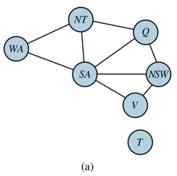
1. Constraint graph for coloring the map of Australia. (b) The map-coloring CSP expressed as a single definite clause. Each map region is represented as a variable whose value can be one of the constants , , or (which are declared ).

Pattern matching

It might seem rather depressing that forward chaining has an NP-hard matching problem in its inner loop. There are three ways to cheer ourselves up:

We can remind ourselves that most rules in real-world knowledge bases are small and simple (like the rules in our crime example) rather than large and complex (like the CSP formulation in Figure 9.5 ). It is common in the database world to assume that both the sizes of rules and the arities of predicates are bounded by a constant and to worry only about data complexity—that is, the complexity of inference as a function of the number of ground facts in the knowledge base. It is easy to show that the data complexity of forward chaining is polynomial, not exponential.

Data complexity

We can consider subclasses of rules for which matching is efficient. Essentially every Datalog clause can be viewed as defining a CSP, so matching will be tractable just when the corresponding CSP is tractable. Chapter 6 describes several tractable families of CSPs. For example, if the constraint graph (the graph whose nodes are variables and whose links are constraints) forms a tree, then the CSP can be solved in linear time. Exactly the same result holds for rule matching. For instance, if we remove South Australia from the map in Figure 9.5 , the resulting clause is

which corresponds to the reduced CSP shown in Figure 6.12 on page 201. Algorithms for solving tree-structured CSPs can be applied directly to the problem of rule matching.

We can try to to eliminate redundant rule-matching attempts in the forward-chaining algorithm, as described next.

Incremental forward chaining

When we showed how forward chaining works on the crime example, we cheated. In particular, we omitted some of the rule matching done by the algorithm shown in Figure 9.3 . For example, on the second iteration, the rule

\[Missile(x) \Rightarrow Weapon(x).\]

matches against (again), and of course the conclusion is already known so nothing happens. Such redundant rule matching can be avoided if we make the following observation: Every new fact inferred on iteration must be derived from at least one new fact inferred on iteration . This is true because any inference that does not require a new fact from iteration could have been done at iteration already.

This observation leads naturally to an incremental forward-chaining algorithm where, at iteration , we check a rule only if its premise includes a conjunct that unifies with a fact newly inferred at iteration . The rule-matching step then fixes to match with , but allows the other conjuncts of the rule to match with facts from any previous iteration. This algorithm generates exactly the same facts at each iteration as the algorithm in Figure 9.3 , but is much more efficient.

With suitable indexing, it is easy to identify all the rules that can be triggered by any given fact, and many real systems operate in an “update” mode wherein forward chaining occurs in response to every TELL. Inferences cascade through the set of rules until the fixed point is reached, and then the process begins again for the next new fact.

Typically, only a small fraction of the rules in the knowledge base are actually triggered by the addition of a given fact. This means that a great deal of redundant work is done in repeatedly constructing partial matches that have some unsatisfied premises. Our crime example is rather too small to show this effectively, but notice that a partial match is constructed on the first iteration between the rule

and the fact . This partial match is then discarded and rebuilt on the second iteration (when the rule succeeds). It would be better to retain and gradually complete the partial matches as new facts arrive, rather than discarding them.

The Rete algorithm was the first to address this problem. The algorithm preprocesses the set of rules in the knowledge base to construct a dataflow network in which each node is a literal from a rule premise. Variable bindings flow through the network and are filtered out when they fail to match a literal. If two literals in a rule share a variable—for example, in the crime example—then the bindings from each literal are filtered through an equality node. A variable binding reaching a node for an -ary literal such as might have to wait for bindings for the other variables to be established before the process can continue. At any given point, the state of a Rete network captures all the partial matches of the rules, avoiding a great deal of recomputation. 3

3 Rete is Latin for net. It rhymes with treaty.

Rete algorithm

Rete networks, and various improvements thereon, have been a key component of so-called production systems, which were among the earliest forward-chaining systems in widespread use. The XCON system (originally called R1; McDermott, 1982) was built with a production-system architecture. XCON contained several thousand rules for designing configurations of computer components for customers of the Digital Equipment Corporation. It was one of the first clear commercial successes in the emerging field of expert systems. Many other similar systems have been built with the same underlying technology, which has been implemented in the general-purpose language OPS-5. 4

4 The word production in production systems denotes a condition–action rule.

Production system

Production systems are also popular in cognitive architectures—that is, models of human reasoning—such as ACT (Anderson, 1983) and SOAR (Laird et al., 1987). In such systems, the “working memory” of the system models human short-term memory, and the productions are part of long-term memory. On each cycle of operation, productions are matched against the working memory of facts. A production whose conditions are satisfied can add or delete facts in working memory. In contrast to the typical situation in databases, production systems often have many rules and relatively few facts. With suitably optimized matching technology, systems can operate in real time with tens of millions of rules.

Cognitive architectures

Irrelevant facts

Another source of inefficiency is that forward chaining makes all allowable inferences based on the known facts, even if they are irrelevant to the goal. In our crime example, there were no rules capable of drawing irrelevant conclusions. But if there had been many rules describe the eating habits of Americans or the components and prices of missiles, then FOL-FC-ASK would have generated irrelevant conclusions.

One way to avoid drawing irrelevant conclusions is to use backward chaining, as described in Section 9.4 . Another way is to restrict forward chaining to a selected subset of rules, as in PL-FC-ENTAILS? (page 231). A third approach has emerged in the field of deductive databases, which are large-scale databases, like relational databases, but which use forward chaining as the standard inference tool rather than SQL queries. The idea is to rewrite the rule set, using information from the goal, so that only relevant variable bindings—those belonging to a so-called magic set—are considered during forward inference. For example, if the goal is , the rule that concludes will be rewritten to include an extra conjunct that constrains the value of :

Deductive databases

Magic set

The fact is also added to the KB. In this way, even if the knowledge base contains facts about millions of Americans, only Colonel West will be considered during the forward inference process. The complete process for defining magic sets and rewriting the knowledge base is too complex to go into here, but the basic idea is to perform a sort of “generic” backward inference from the goal in order to work out which variable bindings need to be constrained. The magic sets approach can therefore be thought of as a kind of hybrid between forward inference and backward preprocessing.

9.4 Backward Chaining

The second major family of logical inference algorithms uses backward chaining over definite clauses. These algorithms work backward from the goal, chaining through rules to find known facts that support the proof.

9.4.1 A backward-chaining algorithm

Figure 9.6 shows a backward-chaining algorithm for definite clauses. FOL-BC-ASK(KB, goal) will be proved if the knowledge base contains a rule of the form , where lhs (left-hand side) is a list of conjuncts. An atomic fact like is considered as a clause whose lhs is the empty list. Now a query that contains variables might be proved in multiple ways. For example, the query could be proved with the substitution as well as with . So we implement FOL-BC-ASK as a generator—a function that returns multiple times, each time giving one possible result (see Appendix B ).

Figure 9.6

A simple backward-chaining algorithm for first-order knowledge bases.

Backward chaining is a kind of AND/OR search—the OR part because the goal query can be proved by any rule in the knowledge base, and the AND part because all the conjuncts in the lhs of a clause must be proved. FOL-BC-OR works by fetching all clauses that might unify with the goal, standardizing the variables in the clause to be brand-new variables, and then, if the rhs of the clause does indeed unify with the goal, proving every conjunct in the lhs, using FOL-BC-AND. That function works by proving each of the conjuncts in turn, keeping track of the accumulated substitution as it goes. Figure 9.7 is the proof tree for deriving from sentences (9.3) through (9.10).

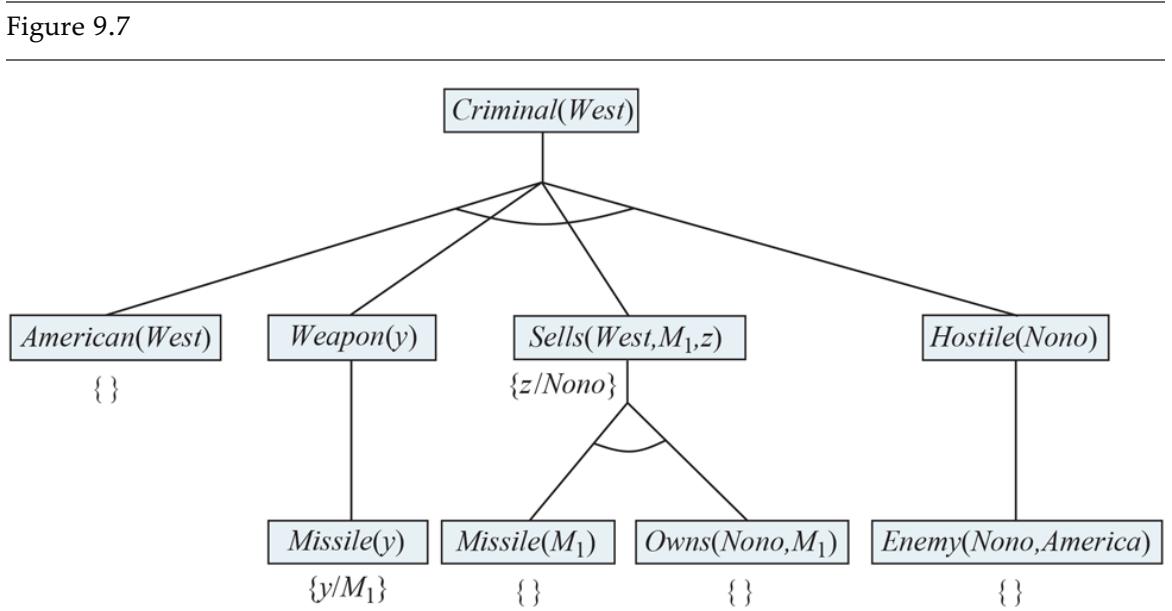
Proof tree constructed by backward chaining to prove that West is a criminal. The tree should be read depth first, left to right. To prove Criminal(West), we have to prove the four conjuncts below it. Some of these are in the knowledge base, and others require further backward chaining. Bindings for each successful unification are shown next to the corresponding subgoal. Note that once one subgoal in a conjunction succeeds, its substitution is applied to subsequent subgoals. Thus, by the time FOL-BC-ASK gets to the last conjunct, originally , is already bound to .

Backward chaining, as we have written it, is clearly a depth-first search algorithm. This means that its space requirements are linear in the size of the proof. It also means that backward chaining (unlike forward chaining) suffers from problems with repeated states and incompleteness. Despite these limitations, backward chaining has proven to be popular and effective in logic programming languages.

9.4.2 Logic programming

Logic programming is a technology that comes close to embodying the declarative ideal described in Chapter 7 : that systems should be constructed by expressing knowledge in a formal language and that problems should be solved by running inference processes on that knowledge. The ideal is summed up in Robert Kowalski’s equation,

\[Algorithm = Logic + Control.\]

Prolog is the most widely used logic programming language. It is used primarily as a rapidprototyping language and for symbol-manipulation tasks such as writing compilers (Van Roy, 1990) and parsing natural language (Pereira and Warren, 1980). Many expert systems have been written in Prolog for legal, medical, financial, and other domains.

Prolog

Prolog programs are sets of definite clauses written in a notation somewhat different from standard first-order logic. Prolog uses uppercase letters for variables and lowercase for constants—the opposite of our convention for logic. Commas separate conjuncts in a clause, and the clause is written “backwards” from what we are used to; instead of in Prolog we have . Here is a typical example:

In Prolog the notation [E|L] denotes a list whose first element is E and whose rest is L. Here is a Prolog program for append(X,Y,Z), which succeeds if list Z is the result of appending lists X and Y:

\[\begin{array}{l}\text{append}([],\mathbf{Y},\mathbf{Y}).\\\text{append}([\mathbf{A}|\mathbf{X}],\mathbf{Y},[\mathbf{A}|\mathbf{Z}]) \mathrel{\mathop{:}}\text{append}(\mathbf{X},\mathbf{Y},\mathbf{Z}).\end{array}\]

In English, we can read these clauses as (1) appending the empty list and the list Y produces the same list Y, and (2) [A|Z] is the result of appending [A|X] and Y, provided that Z is the result of appending X and Y. In most high-level languages we can write a similar recursive function that describes how to append two lists. The Prolog definition is actually more

powerful, however, because it describes a relation that holds among three arguments, rather than a function computed from two arguments. For example, we can ask the query append(X,Y,[1,2,3]): what two lists can be appended to give [1,2,3]? Prolog gives us back the solutions

\[\begin{aligned} \mathbf{X} &= [] & \mathbf{Y} &= [1,2,3]; \\ \mathbf{X} &= [1] & \mathbf{Y} &= [2,3]; \\ \mathbf{X} &= [1,2] & \mathbf{Y} &= [3]; \\ \mathbf{X} &= [1,2,3] & \mathbf{Y} &= [] \end{aligned}\]

The execution of Prolog programs is done through depth-first backward chaining, where clauses are tried in the order in which they are written in the knowledge base. Prolog’s design represents a compromise between declarativeness and execution efficiency. Some aspects of Prolog fall outside standard logical inference:

• Prolog uses the database semantics of Section 8.2.8 rather than first-order semantics, and this is apparent in its treatment of equality and negation (see Section 9.4.4 ).
• There is a set of built-in functions for arithmetic. Literals using these function symbols are “proved” by executing code rather than doing further inference. For example, the goal “X is” succeeds with X bound to 7. On the other hand, the goal “5 is” fails, because the built-in functions do not do arbitrary equation solving.
• There are built-in predicates that have side effects when executed. These include input– output predicates and the assert/retract predicates for modifying the knowledge base. Such predicates have no counterpart in logic and can produce confusing results for example, if facts are asserted in a branch of the proof tree that eventually fails.
• The occur check is omitted from Prolog’s unification algorithm. This means that some unsound inferences can be made; these are almost never a problem in practice.
• Prolog uses depth-first backward-chaining search with no checks for infinite recursion. This makes for a usable programming language that is very fast when used properly, but it means that some programs that look like valid logic will fail to terminate.

9.4.3 Redundant inference and infinite loops

We now turn to the Achilles heel of Prolog: the mismatch between depth-first search and search trees that include repeated states and infinite paths. Consider the following logic program that decides if a path exists between two points on a directed graph:

A simple three-node graph, described by the facts link(a,b) and link(b,c), is shown in Figure 9.8(a) . With this program, the query path(a,c) generates the proof tree shown in Figure 9.9(a) . On the other hand, if we put the two clauses in the order

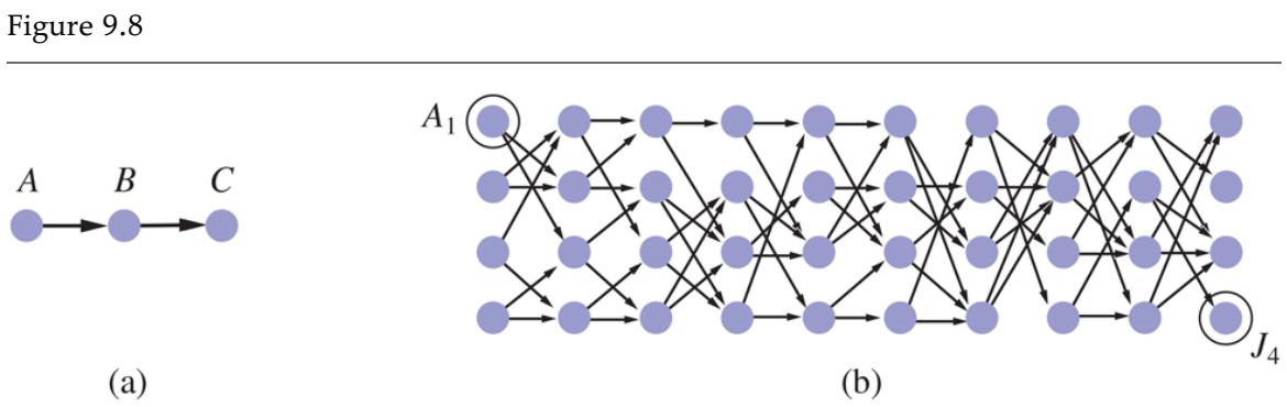
1. Finding a path from to can lead Prolog into an infinite loop. (b) A graph in which each node is connected to two random successors in the next layer. Finding a path from to requires 877 inferences.

Figure 9.9

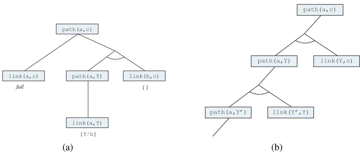
1. Proof that a path exists from to . (b) Infinite proof tree generated when the clauses are in the “wrong” order.

then Prolog follows the infinite path shown in Figure 9.9(b) . Prolog is therefore incomplete as a theorem prover for definite clauses—even for Datalog programs, as this example shows—because, for some knowledge bases, it fails to prove sentences that are entailed. Notice that forward chaining does not suffer from this problem: once path(a,b), path(b,c), and path(a,c) are inferred, forward chaining halts.

Depth-first backward chaining also has problems with redundant computations. For example, when finding a path from to in Figure 9.8(b) , Prolog performs 877 inferences, most of which involve finding all possible paths to nodes from which the goal is unreachable. This is similar to the repeated-state problem discussed in Chapter 3 . The total amount of inference can be exponential in the number of ground facts that are generated. If we apply forward chaining instead, at most path(X,Y) facts can be generated linking nodes. For the problem in Figure 9.8(b) , only 62 inferences are needed.

Forward chaining on graph search problems is an example of dynamic programming, in which the solutions to subproblems are constructed incrementally from those of smaller subproblems and are cached to avoid recomputation. We can obtain a similar effect in a backward chaining system, except that here we are breaking down large goals into smaller ones, rather than building them up.

Dynamic programming

Either way, storing intermediate results to avoid duplication is key. This is the approach taken by tabled logic programming systems, which use efficient storage and retrieval mechanisms. Tabled logic programming combines the goal-directedness of backward chaining with the dynamic-programming efficiency of forward chaining. It is also complete for Datalog knowledge bases, which means that the programmer need worry less about infinite loops. (It is still possible to get an infinite loop with predicates like father(X,Y) that refer to a potentially unbounded number of objects.)

Tabled logic programming

9.4.4 Database semantics of Prolog

Prolog uses database semantics, as discussed in Section 8.2.8 . The unique names assumption says that every Prolog constant and every ground term refers to a distinct object, and the closed world assumption says that the only sentences that are true are those that are entailed by the knowledge base. There is no way to assert that a sentence is false in Prolog. This makes Prolog less expressive than first-order logic, but it is part of what makes Prolog more efficient and more concise. Consider the following assertions about some course offerings:

(9.11)

Under the unique names assumption, CS and EE are different (as are 101, 102, and 106), so this means that there are four distinct courses. Under the closed-world assumption there are no other courses, so there are exactly four courses. But if these were assertions in FOL rather than in database semantics, then all we could say is that there are somewhere between one and infinity courses. That’s because the assertions (in FOL) do not deny the possibility that other unmentioned courses are also offered, nor do they say that the courses mentioned are different from each other. If we wanted to translate Equation (9.11) into FOL, we would get the following sentence:

(9.12)

\[\begin{aligned} \textit{Course}(d, n) &\iff \left(d = CS \land n = 101\right) \lor \left(d = CS \land n = 102\right) \\ \lor \left(d = CS \land n = 106\right) \lor \left(d = EE \land n = 101\right) .\end{aligned}\]

This is called the completion of Equation (9.11) . It expresses in FOL the idea that there are at most four courses. To express in FOL the idea that there are at least four courses, we need to write the completion of the equality predicate:

\[x = y \quad \Leftrightarrow \ (x = CS \land y = CS) \lor (x = EE \land y = EE) \lor (x = 101 \land y = 101)\]

\[\lor (x = 102 \land y = 102) \lor (x = 106 \land y = 106).\]

Completion

The completion is useful for understanding database semantics, but for practical purposes, if your problem can be described with database semantics, it is more efficient to reason with Prolog or some other database semantics system, rather than translating into FOL and reasoning with a full FOL theorem prover.

9.4.5 Constraint logic programming

In our discussion of forward chaining (Section 9.3 ), we showed how constraint satisfaction problems (CSPs) can be encoded as definite clauses. Standard Prolog solves such problems in exactly the same way as the backtracking algorithm given in Figure 6.5 .

Because backtracking enumerates the domains of the variables, it works only for finitedomain CSPs. In Prolog terms, there must be a finite number of solutions for any goal with unbound variables. (For example, a map coloring problem in which each variable can take on one of four different colors.) Infinite-domain CSPs—for example, with integer- or realvalued variables—require quite different algorithms, such as bounds propagation or linear programming.

Consider the following example. We define triangle(X,Y,Z) as a predicate that holds if the three arguments are numbers that satisfy the triangle inequality:

If we ask Prolog the query triangle(3,4,5), it succeeds. On the other hand, if we ask triangle(3,4,Z), no solution will be found, because the subgoal cannot be handled by Prolog; we can’t compare an unbound value to 0.

Constraint logic programming (CLP) allows variables to be constrained rather than bound. A CLP solution is the most specific set of constraints on the query variables that can be derived from the knowledge base. For example, the solution to the triangle(3,4,Z)

query is the constraint . Standard logic programs are just a special case of CLP in which the solution constraints must be equality constraints—that is, bindings.

Constraint logic programming

CLP systems incorporate various constraint-solving algorithms for the constraints allowed in the language. For example, a system that allows linear inequalities on real-valued variables might include a linear programming algorithm for solving those constraints. CLP systems also adopt a much more flexible approach to solving standard logic programming queries. For example, instead of depth-first, left-to-right backtracking, they might use any of the more efficient algorithms discussed in Chapter 6 , including heuristic conjunct ordering, backjumping, cutset conditioning, and so on. CLP systems therefore combine elements of constraint satisfaction algorithms, logic programming, and deductive databases.

Several systems that allow the programmer more control over the search order for inference have been defined. The MRS language (Genesereth and Smith, 1981; Russell, 1985) allows the programmer to write metarules to determine which conjuncts are tried first. The user could write a rule saying that the goal with the fewest variables should be tried first or could write domain-specific rules for particular predicates.

Metarule

9.5 Resolution

The last of our three families of logical systems, and the only one that works for any knowledge base, not just definite clauses, is resolution. We saw on page 223 that propositional resolution is a complete inference procedure for propositional logic; in this section, we extend it to first-order logic.

9.5.1 Conjunctive normal form for first-order logic

The first step is to convert sentences to conjunctive normal form (CNF)—that is, a conjunction of clauses, where each clause is a disjunction of literals. In CNF, literals can contain variables, which are assumed to be universally quantified. For example, the sentence 5

5 A clause can also be represented as an implication with a conjunction of atoms in the premise and a disjunction of atoms in the conclusion (Exercise 9.DISJ). This is called implicative normal form or Kowalski form (especially when written with a right-to-left implication symbol (Kowalski, 1979)) and is generally much easier to read than a disjunction with many negated literals.

becomes, in CNF,

\[\neg Americanan(x) \lor \negWeapon(y) \lor \negSells(x,y,z) \lor \negHostile(z) \lor Criminal(x).\]

The key is that Every sentence of first-order logic can be converted into an inferentially equivalent CNF sentence.

The procedure for conversion to CNF is similar to the propositional case, which we saw on page 226. The principal difference arises from the need to eliminate existential quantifiers. We illustrate the procedure by translating the sentence “Everyone who loves all animals is loved by someone,” or

\[\forall x \; [\forall y \; Animal(y) \Rightarrow Loves(x, y)] \Rightarrow [\exists y \; Loves(y, x)] \; .\]

The steps are as follows:

ELIMINATE IMPLICATIONS: Replace with . For our sample sentence, this needs to be done twice:

MOVE INWARDS: In addition to the usual rules for negated connectives, we need rules for negated quantifiers. Thus, we have

\[ \begin{array}{ccc} \neg \forall x \, p & \text{becomes} & \exists x \, \neg p \\ \neg \exists x \, p & \text{becomes} & \forall x \, \neg p. \end{array} \]

Our sentence goes through the following transformations:

\[\begin{aligned} \forall x \left[ \exists y \quad \neg \left( \neg Animal(y) \lor Loves(x, y) \right) \right] \lor \left[ \exists y \quad \; Loves(y, x) \right]. \\ \forall x \left[ \exists y \quad \neg \neg Animal(y) \land \neg Loves(x, y) \right] \lor \left[ \exists y \quad \; Loves(y, x) \right]. \\ \forall x \left[ \exists y \quad \; Animal(y) \land \neg Loves(x, y) \right] \lor \left[ \exists y \quad \; Loves(y, x) \right]. \end{aligned}\]

Notice how a universal quantifier ( ) in the premise of the implication has become an existential quantifier. The sentence now reads “Either there is some animal that doesn’t love, or (if this is not the case) someone loves .” Clearly, the meaning of the original sentence has been preserved.

STANDARDIZE VARIABLES: For sentences like that use the same variable name twice, change the name of one of the variables. This avoids confusion later when we drop the quantifiers. Thus, we have

\[\forall x \; [\exists y \; \; Animal(y) \land \neg Loves(x, y)] \lor [\exists z \; \; Loves(z, x)].\]

SKOLEMIZE: Skolemization is the process of removing existential quantifiers by elimination. In the simple case, it is just like the Existential Instantiation rule of Section 9.1 : translate into , where is a new constant. However, we can’t apply Existential Instantiation to our sentence above because it doesn’t match the pattern ; only parts of the sentence match the pattern. If we blindly apply the rule to the two matching parts we get

\[\forall x \; [Animal(A) \land \neg Loves(x, A)] \lor Loves(B, x) \; ,\]

which has the wrong meaning entirely: it says that everyone either fails to love a particular animal or is loved by some particular entity . In fact, our original sentence allows each person to fail to love a different animal or to be loved by a different person. Thus, we want the Skolem entities to depend on :

\[\forall x \; [Aini mal(F(x)) \land \neg Loves(x, F(x))] \lor Loves(G(x), x) .\]

Here and are Skolem functions. The general rule is that the arguments of the Skolem function are all the universally quantified variables in whose scope the existential quantifier appears. As with Existential Instantiation, the Skolemized sentence is satisfiable exactly when the original sentence is satisfiable.

Skolem function

DROP UNIVERSAL QUANTIFIERS: At this point, all remaining variables must be universally quantified. Therefore, we don’t lose any information if we drop the quantifier:

DISTRIBUTE OVER :

\[[A\\inmal(F(x)) \lor Looves(G(x),x)] \land [\neg Loves(x,F(x)) \lor Loves(G(x),x)]\]

This step may also require flattening out nested conjunctions and disjunctions.

The sentence is now in CNF and consists of two clauses. It is much more difficult to read than the original sentence with implications. (It may help to explain that the Skolem function refers to the animal potentially unloved by , whereas refers to someone who might love .) Fortunately, humans seldom need to look at CNF sentences—the translation process is easily automated.

9.5.2 The resolution inference rule

The resolution rule for first-order clauses is simply a lifted version of the propositional resolution rule given on page 226. Two clauses, which are assumed to be standardized apart so that they share no variables, can be resolved if they contain complementary literals. Propositional literals are complementary if one is the negation of the other; first-order literals are complementary if one unifies with the negation of the other. Thus, we have

where . For example, we can resolve the two clauses

\[[Animal(F(x)) \lor Looves(G(x), x)] \quad \text{and} \quad [\neg Looves(u, v) \lor \neg Kills(u, v)]\]

by eliminating the complementary literals and , with the unifier , to produce the resolvent clause

\[[A in mathcal{F}(x)) \lor \neg K ll (G(x), x)].\]

This rule is called the binary resolution rule because it resolves exactly two literals. The binary resolution rule by itself does not yield a complete inference procedure. The full resolution rule resolves subsets of literals in each clause that are unifiable. An alternative approach is to extend factoring—the removal of redundant literals—to the first-order case. Propositional factoring reduces two literals to one if they are identical; first-order factoring reduces two literals to one if they are unifiable. The unifier must be applied to the entire clause. The combination of binary resolution and factoring is complete.

Binary resolution

9.5.3 Example proofs

Resolution proves that by proving that unsatisfiable—that is, by deriving the empty clause. The algorithmic approach is identical to the propositional case, described in Figure 7.13 , so we need not repeat it here. Instead, we give two example proofs. The first is the crime example from Section 9.3 . The sentences in CNF are

We also include the negated goal . The resolution proof is shown in Figure 9.10 . Notice the structure: single “spine” beginning with the goal clause, resolving against clauses from the knowledge base until the empty clause is generated. This is characteristic of resolution on Horn clause knowledge bases. In fact, the clauses along the main spine correspond exactly to the consecutive values of the goals variable in the backward-chaining algorithm of Figure 9.6 . This is because we always choose to resolve with a clause whose positive literal unifies with the leftmost literal of the “current” clause on the spine; this is exactly what happens in backward chaining. Thus, backward chaining is just a special case of resolution with a particular control strategy to decide which resolution to perform next.

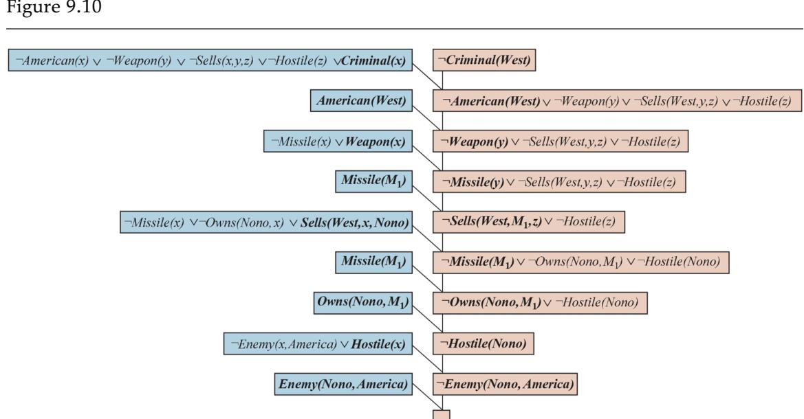
A resolution proof that West is a criminal. At each resolution step, the literals that unify are in bold and the clause with the positive literal is shaded blue.

Our second example makes use of Skolemization and involves clauses that are not definite clauses. This results in a somewhat more complex proof structure. In English:

Everyone who loves all animals is loved by someone.

Anyone who kills an animal is loved by no one.

Jack loves all animals.

Either Jack or Curiosity killed the cat, who is named Tuna.

Did Curiosity kill the cat?

First, we express the original sentences, some background knowledge, and the negated goal G in first-order logic:

Now we apply the conversion procedure to convert each sentence to CNF:

The resolution proof that Curiosity killed the cat is given in Figure 9.11 . In English, the proof could be paraphrased as follows:

Suppose Curiosity did not kill Tuna. We know that either Jack or Curiosity did; thus Jack must have. Now, Tuna is a cat and cats are animals, so Tuna is an animal. Because anyone who kills an animal is loved by no one, we know that no one loves Jack. On the other hand, Jack loves all animals, so someone loves him; so we have a contradiction. Therefore, Curiosity killed the cat.

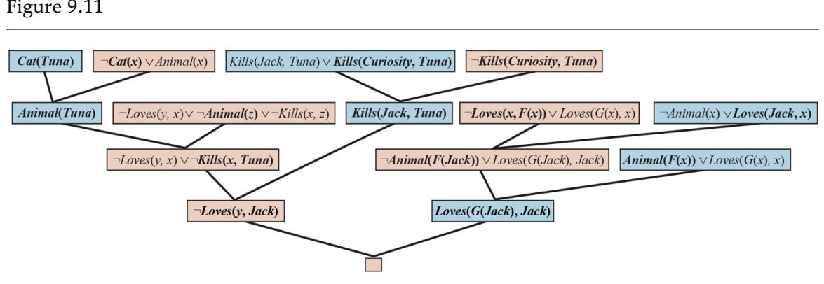
A resolution proof that Curiosity killed the cat. Notice the use of factoring in the derivation of the clause . Notice also in the upper right, the unification of and can only succeed after the variables have been standardized apart.

The proof answers the question “Did Curiosity kill the cat?” but often we want to pose more general questions, such as “Who killed the cat?” Resolution can do this, but it takes a little more work to obtain the answer. The goal is , which, when negated, becomes in CNF. Repeating the proof in Figure 9.11 with the new negated goal, we obtain a similar proof tree, but with the substitution in one of the steps. So, in this case, finding out who killed the cat is just a matter of keeping track of the bindings for the query variables in the proof. Unfortunately, resolution can sometimes produce nonconstructive proofs for existential goals, where we know a query is true, but there isn’t a unique binding for the variable.

Nonconstructive proof

9.5.4 Completeness of resolution

This section gives a completeness proof of resolution. It can be safely skipped by those who are willing to take it on faith.

We show that resolution is refutation-complete, which means that if a set of sentences is unsatisfiable, then resolution will always be able to derive a contradiction. Resolution cannot be used to generate all logical consequences of a set of sentences, but it can be used to establish that a given sentence is entailed by the set of sentences. Hence, it can be used to find all answers to a given question, , by proving that is unsatisfiable.

Refutation completeness

We take it as given that any sentence in first-order logic (without equality) can be rewritten as a set of clauses in CNF. This can be proved by induction on the form of the sentence, using atomic sentences as the base case (Davis and Putnam, 1960). Our goal therefore is to prove the following: if is an unsatisfiable set of clauses, then the application of a finite number of resolution steps to will yield a contradiction.

Our proof sketch follows Robinson’s original proof with some simplifications from Genesereth and Nilsson (1987). The basic structure of the proof (Figure 9.12 ) is as follows:

• 1. First, we observe that if is unsatisfiable, then there exists a particular set of ground instances of the clauses of such that this set is also unsatisfiable (Herbrand’s theorem).
• 2. We then appeal to the ground resolution theorem given in Chapter 7 , which states that propositional resolution is complete for ground sentences.
• 3. We then use a lifting lemma to show that, for any propositional resolution proof using the set of ground sentences, there is a corresponding first-order resolution proof using the first-order sentences from which the ground sentences were obtained.

Figure 9.12

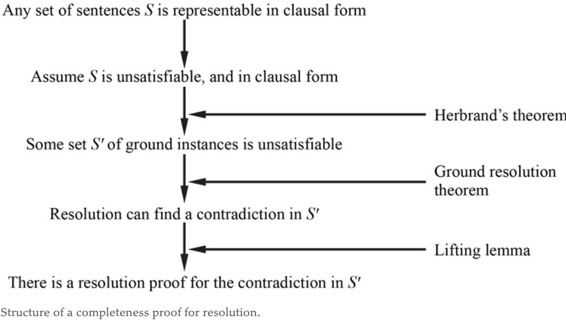
To carry out the first step, we need three new concepts:

• HERBRAND UNIVERSE: If is a set of clauses, then , the Herbrand universe of , is the set of all ground terms constructible from the following:
  • a. The function symbols in , if any.
  • b. The constant symbols in , if any; if none, then a default constant symbol, .

Herbrand universe

For example, if contains just the clause , then is the following infinite set of ground terms:

SATURATION: If is a set of clauses and is a set of ground terms, then , the saturation of with respect to , is the set of all ground clauses obtained by applying all possible consistent substitutions of ground terms in for variables in .

Saturation

HERBRAND BASE: The saturation of a set of clauses with respect to its Herbrand universe is called the Herbrand base of , written as . For example, if contains solely the clause given above, then is the infinite set of clauses

\[\begin{aligned} &\{\neg P(A, F(A, A)) \lor \neg Q(A, A) \lor R(A, B), \\ &\neg P(B, F(B, A)) \lor \neg Q(B, A) \lor R(B, B), \\ &\neg P(F(A, A), F(F(A, A), A)) \lor \neg Q(F(A, A), A) \lor R(F(A, A), B), \\ &\neg P(F(A, B), F(F(A, B), A)) \lor \neg Q(F(A, B), A) \lor R(F(A, B), B), \ldots \} \end{aligned}\]

Herbrand base

These definitions allow us to state a form of Herbrand’s theorem (Herbrand, 1930):

If a set of clauses is unsatisfiable, then there exists a finite subset of that is also unsatisfiable.

Herbrand’s theorem

Let be this finite subset of ground sentences. Now, we can appeal to the ground resolution theorem (page 228) to show that the resolution closure contains the empty clause. That is, running propositional resolution to completion on will derive a contradiction.

Now that we have established that there is always a resolution proof involving some finite subset of the Herbrand base of , the next step is to show that there is a resolution proof using the clauses of itself, which are not necessarily ground clauses. We start by considering a single application of the resolution rule. Robinson stated this lemma:

Let and be two clauses with no shared variables, and let and be ground instances of and . If is a resolvent of and , then there exists a clause such that (1) is a resolvent of and and (2) is a ground instance of .

Gödel’s Incompleteness Theorem

By slightly extending the language of first-order logic to allow for the mathematical induction schema in arithmetic, Kurt Gödel was able to show, in his incompleteness theorem, that there are true arithmetic sentences that cannot be proved.

The proof of the incompleteness theorem is somewhat beyond the scope of this book, occupying, as it does, at least 30 pages, but we can give a hint here. We begin with the logical theory of numbers. In this theory, there is a single constant, 0, and a single function, (the successor function). In the intended model, denotes 1, denotes 2, and so on; the language therefore has names for all the natural numbers. The vocabulary also includes the function symbols , , and (exponentiation) and the usual set of logical connectives and quantifiers.

The first step is to notice that the set of sentences that we can write in this language can be enumerated. (Imagine defining an alphabetical order on the symbols and then arranging, in alphabetical order, each of the sets of sentences of length 1, 2, and so on.) We can then number each sentence with a unique natural number (the Gödel number). This is crucial: number theory contains a name for each of its own sentences. Similarly, we can number each possible proof with a Gödel number , because a proof is simply a finite sequence of sentences.

Now suppose we have a recursively enumerable set of sentences that are true statements about the natural numbers. Recalling that can be named by a given set of integers, we can imagine writing in our language a sentence of the following sort:

is not the Gödel number of a proof of the sentence whose Gödel number is , where the proof uses only premises in .

Then let be the sentence , that is, a sentence that states its own unprovability from . (That this sentence always exists is true but not entirely obvious.)

Now we make the following ingenious argument: Suppose that is provable from ; then is false (because says it cannot be proved). But then we have a false sentence that is provable from , so cannot consist of only true sentences—a violation of our premise. Therefore, is not provable from . But this is exactly what itself claims; hence is a true sentence.

So, we have shown (barring pages) that for any set of true sentences of number theory, and in particular any set of basic axioms, there are other true sentences that cannot be proved from those axioms. This establishes, among other things, that we can never prove all the theorems of mathematics within any given system of axioms. Clearly, this was an important discovery for mathematics. Its significance for AI has been widely debated, beginning with speculations by Gödel himself. We take up the debate in Chapter 27 .

This is called a lifting lemma, because it lifts a proof step from ground clauses up to general first-order clauses. In order to prove his basic lifting lemma, Robinson had to invent unification and derive all of the properties of most general unifiers. Rather than repeat the proof here, we simply illustrate the lemma:

\[\begin{aligned} C\_1 &= \neg P(x, F(x, A)) \lor \neg Q(x, A) \lor R(x, B) \\ C\_2 &= \neg N(G(y), z) \lor P(H(y), z) \\ C\_1' &= \neg P(H(B), F(H(B), A)) \lor \neg Q(H(B), A) \lor R(H(B), B) \\ C\_2' &= \neg N(G(B), F(H(B), A)) \lor P(H(B), F(H(B), A)) \\ C' &= \neg N(G(B), F(H(B), A)) \lor \neg Q(H(B), A) \lor R(H(B), B) \\ C &= \neg N(G(y), F(H(y), A)) \lor \neg Q(H(y), A) \lor R(H(y), B) \end{aligned}\]

Lifting lemma

We see that indeed is a ground instance of . In general, for and to have any resolvents, they must be constructed by first applying to and the most general unifier of a pair of complementary literals in and . From the lifting lemma, it is easy to derive a similar statement about any sequence of applications of the resolution rule:

For any clause in the resolution closure of there is a clause in the resolution closure of such that is a ground instance of and the derivation of is the same length as the derivation of .

From this fact, it follows that if the empty clause appears in the resolution closure of , it must also appear in the resolution closure of . This is because the empty clause cannot be a ground instance of any other clause. To recap: we have shown that if is unsatisfiable, then there is a finite derivation of the empty clause using the resolution rule.

The lifting of theorem proving from ground clauses to first-order clauses provides a vast increase in power. This increase comes from the fact that the first-order proof need instantiate variables only as far as necessary for the proof, whereas the ground-clause methods were required to examine a huge number of arbitrary instantiations.

9.5.5 Equality

None of the inference methods described so far in this chapter can handle an assertion of the form without some additional work. Three distinct approaches can be taken. The first is to axiomatize equality—to write down sentences about the equality relation in the knowledge base. We need to say that equality is reflexive, symmetric, and transitive, and we also have to say that we can substitute equals for equals in any predicate or function. So we need three basic axioms, and then one for each predicate and function:

Given these sentences, a standard inference procedure such as resolution can perform tasks requiring equality reasoning, such as solving mathematical equations. However, these axioms will generate a lot of conclusions, most of them not helpful to a proof. So the second approach is to add inference rules rather than axioms. The simplest rule, demodulation, takes a unit clause and some clause that contains the term , and yields a new clause formed by substituting for within . It works if the term within unifies with ; it need not be exactly equal to . Note that demodulation is directional; given , the always gets replaced with , never vice versa. That means that demodulation can be used for simplifying expressions using demodulators such as or . As another example, given

we can conclude by demodulation

More formally, we have

DEMODULATION: For any terms , , and , where appears somewhere in literal and where ,

Demodulation

where SUBST is the usual substitution of a binding list, and SUB means to replace with somewhere within .

The rule can also be extended to handle non-unit clauses in which an equal sign appears:

PARAMODULATION: For any terms , , and , where appears somewhere in literal , and where ,

\[\frac{\ell\_1 \lor \cdots \lor \ell\_k \lor x = y, \qquad m\_1 \lor \cdots \lor m\_n}{\text{SUB}(\text{SBSr}(\theta, x), \text{SBSr}(\theta, y), \text{SBSr}(\theta, \ell\_1 \lor \cdots \lor \ell\_k \lor m\_1 \lor \cdots \lor m\_n)}\]

Paramodulation

For example, from

\[P(F(x,B),x) \lor Q(x) \qquad \text{and} \qquad F(A,y) = y \lor R(y)\]

we have , and we can conclude by paramodulation the sentence

\[P(B, A) \lor Q(A) \lor R(B).\]

Paramodulation yields a complete inference procedure for first-order logic with equality.

A third approach handles equality reasoning entirely within an extended unification algorithm. That is, terms are unifiable if they are provably equal under some substitution, where “provably” allows for equality reasoning. For example, the terms and normally are not unifiable, but a unification algorithm that knows that could unify them with the empty substitution. Equational unification of this kind can be done with efficient algorithms designed for the particular axioms used (commutativity, associativity, and so on) rather than through explicit inference with those axioms. Theorem provers using this technique are closely related to the CLP systems described in Section 9.4 .

Equational unification

9.5.6 Resolution strategies

We know that repeated applications of the resolution inference rule will eventually find a proof if one exists. In this subsection, we examine strategies that help find proofs efficiently.

UNIT PREFERENCE: This strategy prefers to do resolutions where one of the sentences is a single literal (also known as a unit clause). The idea behind the strategy is that we are trying to produce an empty clause, so it might be a good idea to prefer inferences that produce shorter clauses. Resolving a unit sentence (such as ) with any other sentence (such as ) always yields a clause (in this case, ) that is shorter than the other clause. When the unit preference strategy was first tried for propositional inference in 1964, it led to a dramatic speedup, making it feasible to prove theorems that could not be handled without the preference. Unit resolution is a restricted form of resolution in which every resolution step must involve a unit clause. Unit resolution is incomplete in general, but complete for Horn clauses. Unit resolution proofs on Horn clauses resemble forward chaining.

Unit preference

The OTTER theorem prover (McCune, 1990), uses a form of best-first search. Its heuristic function measures the “weight” of each clause, where lighter clauses are preferred. The exact choice of heuristic is up to the user, but generally, the weight of a clause should be correlated with its size or difficulty. Unit clauses are treated as light; the search can thus be seen as a generalization of the unit preference strategy.

SET OF SUPPORT: Preferences that try certain resolutions first are helpful, but in general it is more effective to try to eliminate some potential resolutions altogether. For example, we can insist that every resolution step involve at least one element of a special set of clauses the set of support. The resolvent is then added into the set of support. If the set of support is small relative to the whole knowledge base, the search space will be reduced dramatically.

Set of support

To ensure completeness of this strategy, we can choose the set of support so that the remainder of the sentences are jointly satisfiable. For example, one can use the negated query as the set of support, on the assumption that the original knowledge base is consistent. (After all, if it is not consistent, then the fact that the query follows from it is vacuous.) The set-of-support strategy has the additional advantage of generating goaldirected proof trees that are often easy for humans to understand.

INPUT RESOLUTION: In this strategy, every resolution combines one of the input sentences (from the KB or the query) with some other sentence. The proof in Figure 9.10 on page 301 uses only input resolutions and has the characteristic shape of a single “spine” with single sentences combining onto the spine. Clearly, the space of proof trees of this shape is smaller than the space of all proof graphs. In Horn knowledge bases, Modus Ponens is a kind of input resolution strategy, because it combines an implication from the original KB with some other sentences. Thus, it is no surprise that input resolution is complete for knowledge bases that are in Horn form, but incomplete in the general case. The linear resolution strategy is a slight generalization that allows and to be resolved together either if is in the original or if is an ancestor of in the proof tree. Linear resolution is complete.

Input resolution

Linear resolution

SUBSUMPTION: The subsumption method eliminates all sentences that are subsumed by (that is, more specific than) an existing sentence in the KB. For example, if is in the KB, then there is no sense in adding and even less sense in adding . Subsumption helps keep the KB small and thus helps keep the search space small.

Subsumption

Learning: We can improve a theorem prover by learning from experience. Given a collection of previously-proved theorems, train a machine learning system to answer the question: given a set of premises and a goal to prove, what proof steps are similar to steps that were successful in the past? The DEEPHOL system (Bansal et al., 2019) does exactly that, using deep neural networks (see Chapter 21 ) to build models (called embeddings) of goals and premises, and using them to make selections. Training can use both human- and computer-generated proofs as examples, starting from a collection of 10,000 proofs.

Learning

Practical uses of resolution theorem provers

We have shown how first-order logic can represent a simple real-world scenario involving concepts like selling, weapons, and citizenship. But complex real-world scenarios have too much uncertainty and too many unknowns. Logic has proven to be more successful for scenarios involving formal, strictly defined concepts, such as the synthesis and verification of both hardware and software. Theorem-proving research is carried out in the fields of hardware design, programming languages, and software engineering—not just in AI.

Synthesis

Verification

In the case of hardware, the axioms describe the interactions between signals and circuit elements. (See Section 8.4.2 on page 273 for an example.) Logical reasoners designed specially for verification have been able to verify entire CPUs, including their timing properties (Srivas and Bickford, 1990). The AURA theorem prover has been applied to design circuits that are more compact than any previous design (Wojciechowski and Wojcik, 1983).

In the case of software, reasoning about programs is quite similar to reasoning about actions, as in Chapter 7 : axioms describe the preconditions and effects of each statement. The formal synthesis of algorithms was one of the first uses of theorem provers, as outlined by Cordell Green (1969a), who built on earlier ideas by Herbert Simon (1963). The idea is to constructively prove a theorem to the effect that “there exists a program satisfying a certain specification.” Although fully automated deductive synthesis, as it is called, has not yet become feasible for general-purpose programming, hand-guided deductive synthesis has been successful in designing several novel and sophisticated algorithms. Synthesis of special-purpose programs, such as scientific computing code, is also an active area of research.

Similar techniques are now being applied to software verification by systems such as the SPIN model checker (Holzmann, 1997). For example, the Remote Agent spacecraft control program was verified before and after flight (Havelund et al., 2000). The RSA public key encryption algorithm and the Boyer–Moore string-matching algorithm have been verified this way (Boyer and Moore, 1984).

Summary

We have presented an analysis of logical inference in first-order logic and a number of algorithms for doing it.

• A first approach uses inference rules (universal instantiation and existential instantiation) to propositionalize the inference problem. Typically, this approach is slow, unless the domain is small.
• The use of unification to identify appropriate substitutions for variables eliminates the instantiation step in first-order proofs, making the process more efficient in many cases.
• A lifted version of Modus Ponens uses unification to provide a natural and powerful inference rule, generalized Modus Ponens. The forward-chaining and backwardchaining algorithms apply this rule to sets of definite clauses.
• Generalized Modus Ponens is complete for definite clauses, although the entailment problem is semidecidable. For Datalog knowledge bases consisting of function-free definite clauses, entailment is decidable.
• Forward chaining is used in deductive databases, where it can be combined with relational database operations. It is also used in production systems, which perform efficient updates with very large rule sets. Forward chaining is complete for Datalog and runs in polynomial time.
• Backward chaining is used in logic programming systems, which employ sophisticated compiler technology to provide very fast inference. Backward chaining suffers from redundant inferences and infinite loops; these can be alleviated by memoization.
• Prolog, unlike first-order logic, uses a closed world with the unique names assumption and negation as failure. These make Prolog a more practical programming language, but bring it further from pure logic.
• The generalized resolution inference rule provides a complete proof system for firstorder logic, using knowledge bases in conjunctive normal form.
• Several strategies exist for reducing the search space of a resolution system without compromising completeness. One of the most important issues is dealing with equality; we showed how demodulation and paramodulation can be used.
• Efficient resolution-based theorem provers have been used to prove interesting mathematical theorems and to verify and synthesize software and hardware.

Bibliographical and Historical Notes

Gottlob Frege, who developed full first-order logic in 1879, based his system of inference on a collection of valid schemas plus a single inference rule, Modus Ponens. Whitehead and Russell (1910) expounded the so-called rules of passage (the actual term is from Herbrand (1930)) that are used to move quantifiers to the front of formulas. Skolem constants and Skolem functions were introduced, appropriately enough, by Thoralf Skolem (1920). Oddly enough, it was Skolem who introduced the Herbrand universe (Skolem, 1928).

Herbrand’s theorem (Herbrand, 1930) has played a vital role in the development of automated reasoning. Herbrand is also the inventor of unification. Gödel (1930) built on the ideas of Skolem and Herbrand to show that first-order logic has a complete proof procedure. Alan Turing (1936) and Alonzo Church (1936) simultaneously showed, using very different proofs, that validity in first-order logic was not decidable. The excellent text by Enderton (1972) explains all of these results in a rigorous yet understandable fashion.

Abraham Robinson proposed that an automated reasoner could be built using propositionalization and Herbrand’s theorem, and Paul Gilmore (1960) wrote the first program. Davis and Putnam (1960) introduced the propositionalization method of Section 9.1 . Prawitz (1960) developed the key idea of letting the quest for propositional inconsistency drive the search, and generating terms from the Herbrand universe only when they were necessary to establish propositional inconsistency. This idea led John Alan Robinson (no relation) to develop resolution (Robinson, 1965).

Resolution was adopted for question-answering systems by Cordell Green and Bertram Raphael (1968). Early AI implementations put a good deal of effort into data structures that would allow efficient retrieval of facts; this work is covered in AI programming texts (Charniak et al., 1987; Norvig, 1992; Forbus and de Kleer, 1993). By the early 1970s, forward chaining was well established in AI as an easily understandable alternative to resolution. AI applications typically involved large numbers of rules, so it was important to develop efficient rule-matching technology, particularly for incremental updates.

The technology for production systems was developed to support such applications. The production system language OPS-5 (Forgy, 1981; Brownston et al., 1985), incorporating the efficient Rete match process (Forgy, 1982), was used for applications such as the R1 expert system for minicomputer configuration (McDermott, 1982). Kraska et al. (2017) describe how neural nets can learn an efficient indexing scheme for specific data sets.

The SOAR cognitive architecture (Laird et al., 1987; Laird, 2008) was designed to handle very large rule sets—up to a million rules (Doorenbos, 1994). Example applications of SOAR include controlling simulated fighter aircraft (Jones et al., 1998), airspace management (Taylor et al., 2007), AI characters for computer games (Wintermute et al., 2007), and training tools for soldiers (Wray and Jones, 2005).

The field of deductive databases began with a workshop in Toulouse in 1977 attended by experts in logical inference and databases (Gallaire and Minker, 1978). Influential work by Chandra and Harel (1980) and Ullman (1985) led to the adoption of Datalog as a standard language for deductive databases. The development of the magic sets technique for rule rewriting by Bancilhon et al. (1986) allowed forward chaining to borrow the advantage of goal-directedness from backward chaining.

The rise of the Internet led to increased availability of massive online databases. This drove increased interest in integrating multiple databases into a consistentdataspace (Halevy, 2007). Kraska et al. (2017) showed speedups of up to 70% by using machine learning to create learned index structures for efficient data lookup.

Backward chaining for logical inference originated in the PLANNER language (Hewitt, 1969). Meanwhile, in 1972, Alain Colmerauer had developed and implemented Prolog for the purpose of parsing natural language—Prolog’s clauses were intended initially as context-free grammar rules (Roussel, 1975; Colmerauer et al., 1973).

Much of the theoretical background for logic programming was developed by Robert Kowalski at Imperial College London, working with Colmerauer; see Kowalski (1988) and Colmerauer and Roussel (1993) for a historical overview. Efficient Prolog compilers are generally based on the Warren Abstract Machine (WAM) model of computation developed by David H. D. Warren (1983). Van Roy (1990) showed that Prolog programs can be competitive with C programs in terms of speed.

Methods for avoiding unnecessary looping in recursive logic programs were developed independently by Smith et al. (1986) and Tamaki and Sato (1986). The latter paper also included memoization for logic programs, a method developed extensively as tabled logic programming by David S. Warren. Swift and Warren (1994) show how to extend the WAM to handle tabling, enabling Datalog programs to execute an order of magnitude faster than forward-chaining deductive database systems.

Early work on constraint logic programming was done by Jaffar and Lassez (1987). Jaffar et al. (1992) developed the CLP(R) system for handling real-valued constraints. There are now commercial products for solving large-scale configuration and optimization problems with constraint programming; one of the best known is ILOG (Junker, 2003). Answer set programming (Gelfond, 2008) extends Prolog, allowing disjunction and negation.

Texts on logic programming and Prolog include Shoham (1994), Bratko (2009), Clocksin (2003), and Clocksin and Mellish (2003). Prior to 2000, the Journal of Logic Programming was the journal of record; it has been replaced by Theory and Practice of Logic Programming. Logic programming conferences include the International Conference on Logic Programming (ICLP) and the International Logic Programming Symposium (ILPS).

Research into mathematical theorem proving began even before the first complete firstorder systems were developed. Herbert Gelernter’s Geometry Theorem Prover (Gelernter, 1959) used heuristic search methods combined with diagrams for pruning false subgoals and was able to prove some quite intricate results in Euclidean geometry. The demodulation and paramodulation rules for equality reasoning were introduced by Wos et al. (1967) and Wos and Robinson (1968), respectively. These rules were also developed independently in the context of term-rewriting systems (Knuth and Bendix, 1970). The incorporation of equality reasoning into the unification algorithm is due to Gordon Plotkin (1972). Jouannaud and Kirchner (1991) survey equational unification from a term-rewriting perspective. An overview of unification is given by Baader and Snyder (2001).

A number of control strategies have been proposed for resolution, beginning with the unit preference strategy (Wos et al., 1964). The set-of-support strategy was proposed by Wos et al. (1965) to provide a degree of goal-directedness in resolution. Linear resolution first appeared in Loveland (1970). Genesereth and Nilsson (1987, Chapter 5 ) provide an analysis of a wide variety of control strategies. Alemi et al. (2017) show how the DEEPMATH

system uses deep neural nets to select the axioms that are most likely to lead to a proof when handed to a traditional theorem prover. In a sense, the neural net plays the role of the mathematician’s intuition, and the theorem prover plays the role of the mathematician’s technical expertise. (Loos et al., 2017) show that this approach can be extended to help guide the search, allowing more theorems to be proved.

A Computational Logic (Boyer and Moore, 1979) is the basic reference on the Boyer-Moore theorem prover. Stickel (1992) describes the Prolog Technology Theorem Prover (PTTP), which combines Prolog compilation and model elimination. SETHEO (Letz et al., 1992) is another widely used theorem prover based on this approach. LEANTAP (Beckert and Posegga, 1995) is an efficient theorem prover implemented in only 25 lines of Prolog. Weidenbach (2001) describes SPASS, one of the strongest current theorem provers. The most successful theorem prover in recent annual competitions has been VAMPIRE (Riazanov and Voronkov, 2002). The COQ system (Bertot et al., 2004) and the E equational solver (Schulz, 2004) have also proven to be valuable tools for proving correctness.

Theorem provers have been used to automatically synthesize and verify software. Examples include the control software for NASA’s Orion capsule (Lowry, 2008) and other spacecraft (Denney et al., 2006). The design of the FM9001 32-bit microprocessor was proved correct by the NQTHM theorem proving system (Hunt and Brock, 1992).

The Conference on Automated Deduction (CADE) runs an annual contest for automated theorem provers. Sutcliffe (2016) describes the 2016 competition; top-scoring systems include VAMPIRE (Riazanov and Voronkov, 2002), PROVER9 (Sabri, 2015), and an updated version of E (Schulz, 2013). Wiedijk (2003) compares the strength of 15 mathematical provers. TPTP (Thousands of Problems for Theorem Provers) is a library of theoremproving problems, useful for comparing the performance of systems (Sutcliffe and Suttner, 1998; Sutcliffe et al., 2006).

Theorem provers have come up with novel mathematical results that eluded human mathematicians for decades, as detailed in the book Automated Reasoning and the Discovery of Missing Elegant Proofs (Wos and Pieper, 2003). The SAM (Semi-Automated Mathematics) program was the first, proving a lemma in lattice theory (Guard et al., 1969). The AURA program has also answered open questions in several areas of mathematics (Wos and Winker, 1983). The Boyer–Moore theorem prover (Boyer and Moore, 1979) was used by

Natarajan Shankar to construct a formal proof of Gödel’s Incompleteness Theorem (Shankar, 1986). The NUPRL system proved Girard’s paradox (Howe, 1987) and Higman’s Lemma (Murthy and Russell, 1990).

In 1933, Herbert Robbins proposed a simple set of axioms—the Robbins algebra—that appeared to define Boolean algebra, but no proof could be found (despite serious work by Alfred Tarski and others) until EQP (a version of OTTER) computed a proof (McCune, 1997). Benzmüller and Paleo (2013) used a higher-order theorem prover to verify Gödel’s proof of the existence of “God.” The Kepler sphere-packing theorem was proved by Thomas Hales (2005) with the help of some complicated computer calculations, but the proof was not completely accepted until a formal proof was generated with the help of the HOL Light and Isabelle proof assistants (Hales et al., 2017).

Robbins algebra

Many early papers in mathematical logic are collected in From Frege to Gödel: A Source Book in Mathematical Logic (van Heijenoort, 1967). Textbooks geared toward automated deduction include the classic Symbolic Logic and Mechanical Theorem Proving (Chang and Lee, 1973), as well as more recent works by Duffy (1991), Wos et al. (1992), Bibel (1993), and Kaufmann et al. (2000). The principal journal for theorem proving is the Journal of Automated Reasoning; the main conferences are the annual Conference on Automated Deduction (CADE) and the International Joint Conference on Automated Reasoning (IJCAR). The Handbook of Automated Reasoning (Robinson and Voronkov, 2001) collects papers in the field. MacKenzie’s Mechanizing Proof (2004) covers the history and technology of theorem proving for the popular audience.

Chapter 10 Knowledge Representation

In which we show how to represent diverse facts about the real world in a form that can be used to reason and solve problems.

The previous chapters showed how an agent with a knowledge base can make inferences that enable it to act appropriately. In this chapter we address the question of what content to put into such an agent’s knowledge base—how to represent facts about the world. We will use first-order logic as the representation language, but later chapters will introduce different representation formalisms such as hierarchical task networks for reasoning about plans (Chapter 11 ), Bayesian networks for reasoning with uncertainty (Chapter 13 ), Markov models for reasoning over time (Chapter 17 ), and deep neural networks for reasoning about images, sounds, and other data (Chapter 21 ). But no matter what representation you use, the facts about the world still need to be handled, and this chapter gives you a feeling for the issues.

Section 10.1 introduces the idea of a general ontology, which organizes everything in the world into a hierarchy of categories. Section 10.2 covers the basic categories of objects, substances, and measures; Section 10.3 covers events; and Section 10.4 discusses knowledge about beliefs. We then return to consider the technology for reasoning with this content: Section 10.5 discusses reasoning systems designed for efficient inference with categories, and Section 10.6 discusses reasoning with default information.

10.1 Ontological Engineering

In “toy” domains, the choice of representation is not that important; many choices will work. Complex domains such as shopping on the Internet or driving a car in traffic require more general and flexible representations. This chapter shows how to create these representations, concentrating on general concepts—such as Events, Time, Physical Objects, and Beliefs—that occur in many different domains. Representing these abstract concepts is sometimes called ontological engineering.

Ontological engineering

We cannot hope to represent everything in the world, even a 1000-page textbook, but we will leave placeholders where new knowledge for any domain can fit in. For example, we will define what it means to be a physical object, and the details of different types of objects —robots, televisions, books, or whatever—can be filled in later. This is analogous to the way that designers of an object-oriented programming framework (such as the Java Swing graphical framework) define general concepts like Window, expecting users to use these to define more specific concepts like SpreadsheetWindow. The general framework of concepts is called an upper ontology because of the convention of drawing graphs with the general concepts at the top and the more specific concepts below them, as in Figure 10.1 .

Figure 10.1

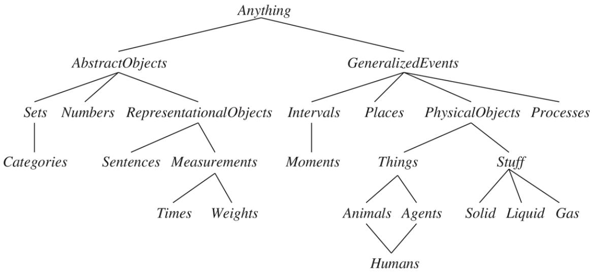
The upper ontology of the world, showing the topics to be covered later in the chapter. Each link indicates that the lower concept is a specialization of the upper one. Specializations are not necessarily disjoint—a human is both an animal and an agent. We will see in Section 10.3.2 why physical objects come under generalized events.

Upper ontology

Before considering the ontology further, we should state one important caveat. We have elected to use first-order logic to discuss the content and organization of knowledge, although certain aspects of the real world are hard to capture in FOL. The principal difficulty is that most generalizations have exceptions or hold only to a degree. For example, although “tomatoes are red” is a useful rule, some tomatoes are green, yellow, or orange. Similar exceptions can be found to almost all the rules in this chapter. The ability to handle exceptions and uncertainty is extremely important, but is orthogonal to the task of understanding the general ontology. For this reason, we delay the discussion of exceptions until Section 10.5 of this chapter, and the more general topic of reasoning with uncertainty until Chapter 12 .

Of what use is an upper ontology? Consider the ontology for circuits in Section 8.4.2 . It makes many simplifying assumptions: time is omitted completely; signals are fixed and do not propagate; the structure of the circuit remains constant. A more general ontology would consider signals at particular times, and would include the wire lengths and propagation

delays. This would allow us to simulate the timing properties of the circuit, and indeed such simulations are often carried out by circuit designers.

We could also introduce more interesting classes of gates, for example, by describing the technology (TTL, CMOS, and so on) as well as the input–output specification. If we wanted to discuss reliability or diagnosis, we would include the possibility that the structure of the circuit or the properties of the gates might change spontaneously. To account for stray capacitances, we would need to represent where the wires are on the board.

If we look at the wumpus world, similar considerations apply. Although we do represent time, it has a simple structure: Nothing happens except when the agent acts, and all changes are instantaneous. A more general ontology, better suited for the real world, would allow for simultaneous changes extended over time. We also used a Pit predicate to say which squares have pits. We could have allowed for different kinds of pits by having several individuals belonging to the class of pits, each having different properties. Similarly, we might want to allow for other animals besides wumpuses. It might not be possible to pin down the exact species from the available percepts, so we would need to build up a biological taxonomy to help the agent predict the behavior of cave dwellers from scanty clues.

For any special-purpose ontology, it is possible to make changes like these to move toward greater generality. An obvious question then arises: do all these ontologies converge on a general-purpose ontology? After centuries of philosophical and computational investigation, the answer is “Maybe.” In this section, we present one general-purpose ontology that synthesizes ideas from those centuries. Two major characteristics of general-purpose ontologies distinguish them from collections of special-purpose ontologies:

• A general-purpose ontology should be applicable in more or less any special-purpose domain (with the addition of domain-specific axioms). This means that no representational issue can be finessed or swept under the carpet.
• In any sufficiently demanding domain, different areas of knowledge must be unified, because reasoning and problem solving could involve several areas simultaneously. A robot circuit-repair system, for instance, needs to reason about circuits in terms of electrical connectivity and physical layout, and about time, both for circuit timing analysis and estimating labor costs. The sentences describing time therefore must be

capable of being combined with those describing spatial layout and must work equally well for nanoseconds and minutes and for angstroms and meters.

We should say up front that the enterprise of general ontological engineering has so far had only limited success. None of the top AI applications (as listed in Chapter 1 ) make use of a general ontology—they all use special-purpose knowledge engineering and machine learning. Social/political considerations can make it difficult for competing parties to agree on an ontology. As Tom Gruber (2004) says, “Every ontology is a treaty—a social agreement —among people with some common motive in sharing.” When competing concerns outweigh the motivation for sharing, there can be no common ontology. The smaller the number of stakeholders, the easier it is to create an ontology, and thus it is harder to create a general-purpose ontology than a limited-purpose one, such as the Open Biomedical Ontology (Smith et al., 2007). Those ontologies that do exist have been created along four routes:

• 1. By a team of trained ontologists or logicians, who architect the ontology and write axioms. The CYC system was mostly built this way (Lenat and Guha, 1990).
• 2. By importing categories, attributes, and values from an existing database or databases. DBPEDIA was built by importing structured facts from Wikipedia (Bizer et al., 2007).
• 3. By parsing text documents and extracting information from them. TEXTRUNNER was built by reading a large corpus of Web pages (Banko and Etzioni, 2008).
• 4. By enticing unskilled amateurs to enter commonsense knowledge. The OPENMIND system was built by volunteers who proposed facts in English (Singh et al., 2002; Chklovski and Gil, 2005).

As an example, the Google Knowledge Graph uses semistructured content from Wikipedia, combining it with other content gathered from across the web under human curation. It contains over 70 billion facts and provides answers for about a third of Google searches (Dong et al., 2014).

10.2 Categories and Objects

The organization of objects into categories is a vital part of knowledge representation. Although interaction with the world takes place at the level of individual objects, much reasoning takes place at the level of categories. For example, a shopper would normally have the goal of buying a basketball, rather than a particular basketball such as . Categories also serve to make predictions about objects once they are classified. One infers the presence of certain objects from perceptual input, infers category membership from the perceived properties of the objects, and then uses category information to make predictions about the objects. For example, from its green and yellow mottled skin, one-foot diameter, ovoid shape, red flesh, black seeds, and presence in the fruit aisle, one can infer that an object is a watermelon; from this, one infers that it would be useful for fruit salad.

Category

There are two choices for representing categories in first-order logic: predicates and objects. That is, we can use the predicate Basketball(b), or we can reify the category as an object, Basketballs. We could then say Member(b,Basketballs), which we will abbreviate as , to say that is a member of the category of basketballs. We say Subset(Basketballs,Balls), abbreviated as , to say that Basketballs is a subcategory of Balls. We will use subcategory, subclass, and subset interchangeably. 1

1 Turning a proposition into an object is called reification, from the Latin word res, or thing. John McCarthy proposed the term “thingification,” but it never caught on.

Reification

Subcategory

Categories organize knowledge through inheritance. If we say that all instances of the category Food are edible, and if we assert that Fruit is a subclass of Food and Apples is a subclass of Fruit, then we can infer that every apple is edible. We say that the individual apples inherit the property of edibility, in this case from their membership in the Food category.

Inheritance

Subclass relations organize categories into a taxonomic hierarchy or taxonomy. Taxonomies have been used explicitly for centuries in technical fields. The largest such taxonomy organizes about 10 million living and extinct species, many of them beetles, into a single hierarchy; library science has developed a taxonomy of all fields of knowledge, encoded as the Dewey Decimal system; and tax authorities and other government departments have developed extensive taxonomies of occupations and commercial products. 2

2 When asked what one could deduce about the Creator from the study of nature, biologist J. B. S. Haldane said “An inordinate fondness for beetles.”

Taxonomic hierarchy

First-order logic makes it easy to state facts about categories, either by relating objects to categories or by quantifying over their members. Here are some example facts:

An object is a member of a category.

• A category is a subclass of another category.
• All members of a category have some properties.
• Members of a category can be recognized by some properties.
• A category as a whole has some properties.

Notice that because Dog is a category and is a member of DomesticatedSpecies, the latter must be a category of categories. Of course there are exceptions to many of the above rules (punctured basketballs are not spherical); we deal with these exceptions later.

Although subclass and member relations are the most important ones for categories, we also want to be able to state relations between categories that are not subclasses of each other. For example, if we just say that Undergraduates and GraduateStudents are subclasses of Students, then we have not said that an undergraduate cannot also be a graduate student. We say that two or more categories are disjoint if they have no members in common. We may also want to say that the classes undergrad and graduate student form an exhaustive decomposition of university students. A exhaustive decomposition of disjoint sets is known as a partition. Here are some more examples of these three concepts:

Disjoint

Exhaustive decomposition

Partition

(Note that the ExhaustiveDecomposition of NorthAmericans is not a Partition, because some people have dual citizenship.) The three predicates are defined as follows:

Categories can also be defined by providing necessary and sufficient conditions for membership. For example, a bachelor is an unmarried adult male:

As we discuss in the sidebar on natural kinds on page 320, strict logical definitions for categories are usually possible only for artificial formal terms, not for ordinary objects. But definitions are not always necessary.

10.2.1 Physical composition

The idea that one object can be part of another is a familiar one. One’s nose is part of one’s head, Romania is part of Europe, and this chapter is part of this book. We use the general PartOf relation to say that one thing is part of another. Objects can be grouped into PartOf hierarchies, reminiscent of the Subset hierarchy:

The PartOf relation is transitive and reflexive; that is,

Composite object

Therefore, we can conclude PartOf (Bucharest,Earth). Categories of composite objects are often characterized by structural relations among parts. For example, a biped is an object with exactly two legs attached to a body:

\[\begin{aligned} Biped(a) &\Rightarrow \exists \, l\_1, l\_2, b \; \begin{aligned} &\exists \, l\_1, l\_2, b \; \begin{aligned} &\mathcal{I} \, \exists \, l\_1 \; \exists \, \mathcal{L}eg(l\_1) \land \mathcal{L}eg(l\_2) \land \mathcal{B}ody(b) \; \land \end{aligned} \\ &\begin{aligned} &\mathcal{A}PartOf(l\_1, a) \land \mathcal{A}PartOf(l\_2, a) \land \mathcal{A}PartOf(b, a) \; \land \\ &\mathcal{A} \, \forall tached(l\_1, b) \land \mathcal{A} \, \forall tached(l\_2, b) \; \land \end{aligned} \\ &\begin{aligned} l\_1 \neq l\_2 \land \left[ \forall l\_3 \; \; \mathcal{L}eg(l\_3) \land \mathcal{A} \, \forall toolof(l\_3, a) \; \Rightarrow \; \left( l\_3 = l\_1 \lor l\_3 = l\_2 \right) \right] \end{aligned} \end{aligned}\]

The notation for “exactly two” is a little awkward; we are forced to say that there are two legs, that they are not the same, and that if anyone proposes a third leg, it must be the same as one of the other two. In Section 10.5.2 , we describe a formalism called description logic that makes it easier to represent constraints like “exactly two.”

We can define a PartPartition relation analogous to the Partition relation for categories. (See Exercise 10.DECM.) An object is composed of the parts in its PartPartition and can be viewed as deriving some properties from those parts. For example, the mass of a composite object is the sum of the masses of the parts. Notice that this is not the case with categories, which have no mass, even though their elements might.

It is also useful to define composite objects with definite parts but no particular structure. For example, we might want to say “The apples in this bag weigh two pounds.” The temptation would be to ascribe this weight to the set of apples in the bag, but this would be a mistake because the set is an abstract mathematical concept that has elements but does not have weight. Instead, we need a new concept, which we will call a bunch. For example, if the apples are , , and , then

denotes the composite object with the three apples as parts (not elements). We can then use the bunch as a normal, albeit unstructured, object. Notice that . Furthermore, BunchOf (Apples) is the composite object consisting of all apples—not to be confused with Apples, the category or set of all apples.

We can define BunchOf in terms of the PartOf relation. Obviously, each element of is part of BunchOf (s):

\[\forall x \quad \quad x \in s \Rightarrow PartOf(x, BunchOf(s)) \;. \; .\]

Furthermore, BunchOf (s) is the smallest object satisfying this condition. In other words, BunchOf (s) must be part of any object that has all the elements of as parts:

\[\forall y \qquad \left[ \forall x \qquad x \in s \Rightarrow PartOf(x, y) \right] \Rightarrow PartOf(BunchOf(s), y) \; .\]

These axioms are an example of a general technique called logical minimization, which means defining an object as the smallest one satisfying certain conditions.

Logical minimization

10.2.2 Measurements

In both scientific and commonsense theories of the world, objects have height, mass, cost, and so on. The values that we assign for these properties are called measures. Ordinary quantitative measures are quite easy to represent. We imagine that the universe includes abstract “measure objects,” such as the length that is the length of this line segment: . We can call this length 1.5 inches or 3.81 centimeters. Thus, the same length has different names in our language. We represent the length with a units function that takes a number as argument. (An alternative is explored in Exercise 10.ALTM.)

Measure

Units function

Natural Kinds

Some categories have strict definitions: an object is a triangle if and only if it is a polygon with three sides. On the other hand, most categories in the real world have no clear-cut definition; these are called natural kind categories. For example, tomatoes tend to be a dull scarlet; roughly spherical; with an indentation at the top where the stem was; about two to four inches in diameter; with a thin but tough skin; and with flesh, seeds, and juice inside. However, there is variation: some tomatoes are yellow or orange, unripe tomatoes are green, some are smaller or larger than average, and cherry tomatoes are uniformly small. Rather than having a complete definition of tomatoes, we have a set of features that serves to identify objects that are clearly typical tomatoes, but might not definitively identify other objects. (Could there be a tomato that is fuzzy like a peach?)

This poses a problem for a logical agent. The agent cannot be sure that an object it has perceived is a tomato, and even if it were sure, it could not be certain which of the properties of typical tomatoes this one has. This problem is an inevitable consequence of operating in partially observable environments.

One useful approach is to separate what is true of all instances of a category from what is true only of typical instances. So in addition to the category Tomatoes, we will also have the category Typical(Tomatoes). Here, the Typical function maps a category to the subclass that contains only typical instances:

Most knowledge about natural kinds will actually be about their typical instances:

Thus, we can write down useful facts about categories without exact definitions. The difficulty of providing exact definitions for most natural categories was

explained in depth by Wittgenstein (1953). He used the example of games to show that members of a category shared “family resemblances” rather than necessary and sufficient characteristics: what strict definition encompasses chess, tag, solitaire, and dodgeball?

The utility of the notion of strict definition was also challenged by Quine (1953). He pointed out that even the definition of “bachelor” as an unmarried adult male is suspect; one might, for example, question a statement such as “the Pope is a bachelor.” While not strictly false, this usage is certainly infelicitous because it induces unintended inferences on the part of the listener. The tension could perhaps be resolved by distinguishing between logical definitions suitable for internal knowledge representation and the more nuanced criteria for felicitous linguistic usage. The latter may be achieved by “filtering” the assertions derived from the former. It is also possible that failures of linguistic usage serve as feedback for modifying internal definitions, so that filtering becomes unnecessary.

If the line segment is called , we can write

Conversion between units is done by equating multiples of one unit to another:

Similar axioms can be written for pounds and kilograms, seconds and days, and dollars and cents. Measures can be used to describe objects as follows:

Note that is not a dollar bill—it is a price. One can have two dollar bills, but there is only one object named . Note also that, while Inches(0) and Centimeters(0) refer to the same zero length, they are not identical to other zero measures, such as Seconds(0).

Simple, quantitative measures are easy to represent. Other measures present more of a problem, because they have no agreed scale of values. Exercises have difficulty, desserts have deliciousness, and poems have beauty, yet numbers cannot be assigned to these qualities. One might, in a moment of pure accountancy, dismiss such properties as useless for the purpose of logical reasoning; or, still worse, attempt to impose a numerical scale on beauty. This would be a grave mistake, because it is unnecessary. The most important aspect of measures is not the particular numerical values, but the fact that measures can be ordered.

Although measures are not numbers, we can still compare them, using an ordering symbol such as . For example, we might well believe that Norvig’s exercises are tougher than Russell’s, and that one scores less on tougher exercises:

This is enough to allow one to decide which exercises to do, even though no numerical values for difficulty were ever used. (One does, however, have to discover who wrote which exercises.) These sorts of monotonic relationships among measures form the basis for the field of qualitative physics, a subfield of AI that investigates how to reason about physical systems without plunging into detailed equations and numerical simulations. Qualitative physics is discussed in the historical notes section.

10.2.3 Objects: Things and stuff

Individuation

Stuff

The real world can be seen as consisting of primitive objects (e.g., atomic particles) and composite objects built from them. By reasoning at the level of large objects such as apples and cars, we can overcome the complexity involved in dealing with vast numbers of primitive objects individually. There is, however, a significant portion of reality that seems to defy any obvious individuation—division into distinct objects. We give this portion the generic name stuff. For example, suppose I have some butter and an aardvark in front of me. I can say there is one aardvark, but there is no obvious number of “butter-objects,” because any part of a butter-object is also a butter-object, at least until we get to very small parts indeed. This is the major distinction between stuff and things. If we cut an aardvark in half, we do not get two aardvarks (unfortunately).

The English language distinguishes clearly between stuff and things. We say “an aardvark,” but, except in pretentious California restaurants, one cannot say “a butter.” Linguists distinguish between count nouns, such as aardvarks, holes, and theorems, and mass nouns, such as butter, water, and energy. Several competing ontologies claim to handle this distinction. Here we describe just one; the others are covered in the historical notes section.

Count nouns

Mass noun

To represent stuff properly, we begin with the obvious. We need to have as objects in our ontology at least the gross “lumps” of stuff we interact with. For example, we might recognize a lump of butter as the one left on the table the night before; we might pick it up, weigh it, sell it, or whatever. In these senses, it is an object just like the aardvark. Let us call it . We also define the category Butter. Informally, its elements will be all those things of which one might say “It’s butter,” including . With some caveats about very small parts that we will omit for now, any part of a butter-object is also a butter-object:

We can now say that butter melts at around 30 degrees centigrade:

\[b ∈ B utter → M leftrightarrow (b, C leftrightarrow (30)) \dots\]

We could go on to say that butter is yellow, is less dense than water, is soft at room temperature, has a high fat content, and so on. On the other hand, butter has no particular size, shape, or weight. We can define more specialized categories of butter such as UnsaltedButter, which is also a kind of stuff. Note that the category PoundOfButter, which includes as members all butter-objects weighing one pound, is not a kind of stuff. If we cut a pound of butter in half, we do not, alas, get two pounds of butter.

What is actually going on is this: some properties are intrinsic: they belong to the very substance of the object, rather than to the object as a whole. When you cut an instance of stuff in half, the two pieces retain the intrinsic properties—things like density, boiling point, flavor, color, ownership, and so on. On the other hand, their extrinsic properties—weight, length, shape, and so on—are not retained under subdivision. A category of objects that includes in its definition only intrinsic properties is then a substance, or mass noun; a class that includes any extrinsic properties in its definition is a count noun. Stuff and Thing are the most general substance and object categories, respectively.

Intrinsic

Extrinsic

10.3 Events

In Section 7.7.1 we discussed actions: things that happen, such as ; and fluents: aspects of the world that change, such as . Both were represented as propositions, and we used successor-state axioms to say that a fluent will be true at time if the action at time caused it to be true, or if it was already true at time and the action did not cause it to be false. That was for a world in which actions are discrete, instantaneous, happen one at a time, and have no variation in how they are performed (that is, there is only one kind of Shoot action, there is no distinction between shooting quickly, slowly, nervously, etc.).

But as we move from simplistic domains to the real world, there is a much richer range of actions or events to deal with. Consider a continuous action, such as filling a bathtub. A successor-state axiom can say that the tub is empty before the action and full when the action is done, but it can’t talk about what happens during the action. It also can’t easily describe two actions happening at the same time—such as brushing one’s teeth while waiting for the tub to fill. To handle such cases we introduce an approach known as event calculus. 3

3 The terms “event” and “action” may be used interchangeably—they both mean “something that can happen.”

Event calculus

The objects of event calculus are events, fluents, and time points. At(Shankar,Berkeley) is a fluent: an object that refers to the fact of Shankar being in Berkeley. The event of Shankar flying from San Francisco to Washington, D.C., is described as

where Flyings is the category of all flying events. By reifying events we make it possible to add any amount of arbitrary information about them. For example, we can say that

Shankar’s flight was bumpy with . In an ontology where events are predicates, there would be no way to add extra information like this; moving to an predicate isn’t a scalable solution.

To assert that a fluent is actually true starting at some point in time and continuing to time , we use the predicate , as in . Similarly, we use to say that the event actually happened, starting at time and ending at time . The complete set of predicates for one version of the event calculus is: 4

4 Our version is based on Shanahan (1999), but with some alterations.

T (f,t1,t2)	Fluent fis true for all times between t1 and t2
Happens (e, t1, t2)	Event e starts at time t1 and ends at t2
Initiates (e, f,t)	Event e causes fluent f to become true at time t
Terminates (e, f,t)	Event e causes fluent f to cease to be true at time t
Initiated (f,t1,t2)	Fluent f become true at some point between t1 and t2
	Terminated (f, t1, t2) Fluent f cease to be true at some point between t2 and t2
ty < t2	Time point t1 occurs before time t2

We can describe the effects of a flying event:

$$E = F triangleright (a, here, there) and Happy (E, t_1, t_2)

Terminates (E, At (a, here), t_1) Intitates (E, At (a, there), t_2)$$

We assume a distinguished event, Start, that describes the initial state by saying which fluents are true (using Initiates) or false (using Terminated) at the start time. We can then describe what fluents are true at what points in time with a pair of axioms for and that follow the same general format as the successor-state axioms: Assume an event happens between time and , and at somewhere in that time interval the event changes the value of fluent , either initiating it (making it true) or terminating it (making it false). Then at time in the future, if no other intervening event has changed the fluent (either terminated or initiated it, respectively), then the fluent will have maintained its value. Formally, the axioms are:

where Terminated and Initiated are defined by:

\[\begin{aligned} &Terminated \left(f, t\_1, t\_5\right) \Leftrightarrow \\ &\exists e, t\_2, t\_3, t\_4 \, Happy \left(e, t\_2, t\_4\right) \land Terminates \left(e, f, t\_3\right) \land t\_1 \leq t\_2 \leq t\_3 \leq t\_4 \leq t\_5 \\ &\exists e, t\_2, t\_3, t\_4 \, Happy \left(e, t\_2, t\_4\right) \land Intitates \left(e, f, t\_3\right) \land t\_1 \leq t\_2 \leq t\_3 \leq t\_4 \leq t\_5 \end{aligned}\]

We can extend event calculus to represent simultaneous events (such as two people being necessary to ride a seesaw), exogenous events (such as the wind moving an object), continuous events (such as the rising of the tide), nondeterministic events (such as flipping a coin and having it come up heads or tails), and other complications.

10.3.1 Time

Event calculus opens us up to the possibility of talking about time points and time intervals. We will consider two kinds of time intervals: moments and extended intervals. The distinction is that only moments have zero duration:

Next we invent a time scale and associate points on that scale with moments, giving us absolute times. The time scale is arbitrary; we will measure it in seconds and say that the moment at midnight (GMT) on January 1, 1900, has time 0. The functions Begin and End pick out the earliest and latest moments in an interval, and the function Time delivers the point on the time scale for a moment. The function Duration gives the difference between the end time and the start time.

To make these numbers easier to read, we also introduce a function Date, which takes six arguments (hours, minutes, seconds, day, month, and year) and returns a time point:

Two intervals Meet if the end time of the first equals the start time of the second. The complete set of interval relations (Allen, 1983) is shown below and in Figure 10.2 :

	Meet (i, j) = = End (i) = Begin (j)
	Before (i, j) = End (i) < Begin (j)
After (j,i) = = Before (i, j)
	During (i, j)
	Overlap (i, j)
	Starts (i, j) = < Begin (i) = Begin (j)
	Finishes (i, j)
	Equals (i, j)

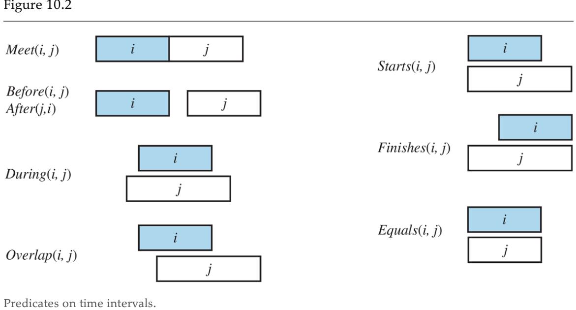
These all have their intuitive meaning, with the exception of Overlap: we tend to think of overlap as symmetric (if overlaps then overlaps ), but in this definition, only is true if begins before . Experience has shown that this definition is more useful for writing axioms. To say that the reign of Elizabeth II immediately followed that of George VI, and the reign of Elvis overlapped with the 1950s, we can write the following:

10.3.2 Fluents and objects

Physical objects can be viewed as generalized events, in the sense that a physical object is a chunk of space–time. For example, USA can be thought of as an event that began in 1776 as a union of 13 states and is still in progress today as a union of 50. We can describe the changing properties of USA using state fluents, such as Population(USA). A property of USA that changes every four or eight years, barring mishaps, is its president. One might propose that President(USA) is a logical term that denotes a different object at different times.

Unfortunately, this is not possible, because a term denotes exactly one object in a given model structure. (The term President(USA, ) can denote different objects, depending on the value of , but our ontology keeps time indices separate from fluents.) The only possibility is that President(USA) denotes a single object that consists of different people at different times. It is the object that is George Washington from 1789 to 1797, John Adams from 1797 to 1801, and so on, as in Figure 10.3 . To say that George Washington was president throughout 1790, we can write

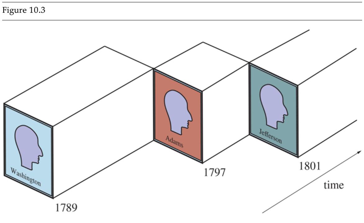
A schematic view of the object President(USA) for the early years.

We use the function symbol Equals rather than the standard logical predicate , because we cannot have a predicate as an argument to , and because the interpretation is not that GeorgeWashington and President(USA) are logically identical in 1790; logical identity is not something that can change over time. The identity is between the subevents of the objects President(USA) and GeorgeWashington that are defined by the period 1790.

10.4 Mental Objects and Modal Logic

The agents we have constructed so far have beliefs and can deduce new beliefs. Yet none of them has any knowledge about beliefs or about deduction. Knowledge about one’s own knowledge and reasoning processes is useful for controlling inference. For example, suppose Alice asks “what is the square root of 1764” and Bob replies “I don’t know.” If Alice insists “think harder,” Bob should realize that with some more thought, this question can in fact be answered. On the other hand, if the question were “Is the president sitting down right now?” then Bob should realize that thinking harder is unlikely to help. Knowledge about the knowledge of other agents is also important; Bob should realize that the president does know.

What we need is a model of the mental objects that are in someone’s head (or something’s knowledge base) and of the mental processes that manipulate those mental objects. The model does not have to be detailed. We do not have to be able to predict how many milliseconds it will take for a particular agent to make a deduction. We will be happy just to be able to conclude that mother knows whether or not she is sitting.

We begin with the propositional attitudes that an agent can have toward mental objects: attitudes such as Believes, Knows, Wants, and Informs. The difficulty is that these attitudes do not behave like “normal” predicates. For example, suppose we try to assert that Lois knows that Superman can fly:

Propositional attitude

One minor issue with this is that we normally think of CanFly(Superman) as a sentence, but here it appears as a term. That issue can be patched up by reifying CanFly(Superman); making it a fluent. A more serious problem is that, if it is true that Superman is Clark Kent,

then we must conclude that Lois knows that Clark can fly, which is wrong because (in most versions of the story) Lois does not know that Clark is Superman.

\[\begin{aligned} &\left(Superman = Color\right) \land Knows \left(Lois, CanFly\left(Superman\right)\right) \\ &= Knows \left(Lois, CanFly\left(Chark\right)\right) \end{aligned}\]

This is a consequence of the fact that equality reasoning is built into logic. Normally that is a good thing; if our agent knows that and , then we want our agent to know that . This property is called referential transparency—it doesn’t matter what term a logic uses to refer to an object, what matters is the object that the term names. But for propositional attitudes like believes and knows, we would like to have referential opacity—the terms used do matter, because not all agents know which terms are co-referential.

Referential transparency

We could patch this up with even more reification: we could have one object to represent Clark/Superman, another object to represent the person that Lois knows as Clark, and yet another for the person Lois knows as Superman. However, this proliferation of objects means that the sentences we want to write quickly become verbose and clumsy.

Modal logic is designed to address this problem. Regular logic is concerned with a single modality, the modality of truth, allowing us to express ” is true” or ” is false.” Modal logic includes special modal operators that take sentences (rather than terms) as arguments. For example, ” knows ” is represented with the notation , where is the modal operator for knowledge. It takes two arguments, an agent (written as the subscript) and a sentence. The syntax of modal logic is the same as first-order logic, except that sentences can also be formed with modal operators.

Modal logic

Modal operators

The semantics of modal logic is more complicated. In first-order logic a model contains a set of objects and an interpretation that maps each name to the appropriate object, relation, or function. In modal logic we want to be able to consider both the possibility that Superman’s secret identity is Clark and the possibility that it isn’t.

Therefore, we will need a more complicated model, one that consists of a collection of possible worlds rather than just one true world. The worlds are connected in a graph by accessibility relations, one relation for each modal operator. We say that world is accessible from world with respect to the modal operator if everything in is consistent with what knows in . As an example, in the real world, Bucharest is the capital of Romania, but for an agent that did not know that, a world where the capital of Romania is, say, Sofia is accessible. Hopefully a world where would not be accessible to any agent.

Possible world

Accessibility relation

In general, a knowledge atom is true in world if and only if is true in every world accessible from . The truth of more complex sentences is derived by recursive application of this rule and the normal rules of first-order logic. That means that modal logic can be used to reason about nested knowledge sentences: what one agent knows about another agent’s knowledge. For example, we can say that even though Lois doesn’t know whether Superman’s secret identity is Clark Kent, she does know that Clark knows:

Modal logic solves some tricky issues with the interplay of quantifiers and knowledge. The English sentence “Bond knows that someone is a spy” is ambiguous. The first reading is that there is a particular someone who Bond knows is a spy; we can write this as

\[ \exists x \quad \mathbf{K}\_{Bond} Spy(x), \]

which in modal logic means that there is an that, in all accessible worlds, Bond knows to be a spy. The second reading is that Bond just knows that there is at least one spy:

\[\mathbf{K}\_{Bond} \exists x \qquad Spy(x) \; .\]

The modal logic interpretation is that in each accessible world there is an that is a spy, but it need not be the same in each world.

Now that we have a modal operator for knowledge, we can write axioms for it. First, we can say that agents are able to draw conclusions; if an agent knows and knows that implies , then the agent knows :

\[(\mathbf{K}\_a P \land \mathbf{K}\_a (P \Rightarrow Q)) \quad \Rightarrow \mathbf{K}\_a Q \dots\]

From this (and a few other rules about logical identities) we can establish that is a tautology; every agent knows every proposition is either true or false. On the other hand, is not a tautology; in general, there will be lots of propositions that an agent does not know to be true and does not know to be false.

It is said (going back to Plato) that knowledge is justified true belief. That is, if it is true, if you believe it, and if you have an unassailably good reason, then you know it. That means that if you know something, it must be true, and we have the axiom:

\[\mathbf{K}\_a P \Rightarrow P\]

Furthermore, logical agents (but not all people) are able to introspect on their own knowledge. If they know something, then they know that they know it:

\[ \mathbf{K}\_a P \Rightarrow \mathbf{K}\_a (\mathbf{K}\_a P)\ . \]

We can define similar axioms for belief (often denoted by ) and other modalities. However, one problem with the modal logic approach is that it assumes logical omniscience on the part of agents. That is, if an agent knows a set of axioms, then it knows all consequences of those axioms. This is on shaky ground even for the somewhat abstract notion of knowledge, but it seems even worse for belief, because belief has more connotation of referring to things that are physically represented in the agent, not just potentially derivable.

Logical omniscience

There have been attempts to define a form of limited rationality for agents—to say that agents believe only those assertions that can be derived with the application of no more than reasoning steps, or no more than seconds of computation. These attempts have been generally unsatisfactory.

10.4.1 Other modal logics

Many modal logics have been proposed, for different modalities besides knowledge. One proposal is to add modal operators for possibility and necessity: it is possibly true that one of the authors of this book is sitting down right now, and it is necessarily true that .

As mentioned in Section 8.1.2 , some logicians favor modalities related to time. In linear temporal logic, we add the following modal operators:

• : ” will be true in the next time step”
• : ” will eventually (Finally) be true in some future time step”
• : ” is always (Globally) true”
• : ” remains true until occurs”

Linear temporal logic

Sometimes there are additional operators that can be derived from these. Adding these modal operators makes the logic itself more complex (and thus makes it harder for a logical inference algorithm to find a proof). But the operators also allow us to state certain facts in a more succinct form (which makes logical inference faster). The choice of which logic to use is similar to the choice of which programming language to use: pick one that is appropriate to your task, that is familiar to you and the others who will share your work, and that is efficient enough for your purposes.

10.5 Reasoning Systems for Categories

Categories are the primary building blocks of large-scale knowledge representation schemes. This section describes systems specially designed for organizing and reasoning with categories. There are two closely related families of systems: semantic networks provide graphical aids for visualizing a knowledge base and efficient algorithms for inferring properties of an object on the basis of its category membership; and description logics provide a formal language for constructing and combining category definitions and efficient algorithms for deciding subset and superset relationships between categories.

Semantic networks

Description logics

10.5.1 Semantic networks

In 1909, Charles S. Peirce proposed a graphical notation of nodes and edges called existential graphs that he called “the logic of the future.” Thus began a long-running debate between advocates of “logic” and advocates of “semantic networks.” Unfortunately, the debate obscured the fact that semantic networks are a form of logic. The notation that semantic networks provide for certain kinds of sentences is often more convenient, but if we strip away the “human interface” issues, the underlying concepts—objects, relations, quantification, and so on—are the same.

Existential graphs

There are many variants of semantic networks, but all are capable of representing individual objects, categories of objects, and relations among objects. A typical graphical notation displays object or category names in ovals or boxes, and connects them with labeled links. For example, Figure 10.4 has a MemberOf link between Mary and FemalePersons, corresponding to the logical assertion ; similarly, the SisterOf link between Mary and John corresponds to the assertion SisterOf (Mary,John). We can connect categories using SubsetOf links, and so on. It is such fun drawing bubbles and arrows that one can get carried away. For example, we know that persons have female persons as mothers, so can we draw a HasMother link from Persons to FemalePersons? The answer is no, because HasMother is a relation between a person and his or her mother, and categories do not have mothers. 5

5 Several early systems failed to distinguish between properties of members of a category and properties of the category as a whole. This can lead directly to inconsistencies, as pointed out by Drew McDermott (1976) in his article “Artificial Intelligence Meets Natural Stupidity.” Another common problem was the use of ISA links for both subset and membership relations, in correspondence with English usage: “a cat is a mammal” and “Fifi is a cat.” See Exercise 10.NATS for more on these issues.

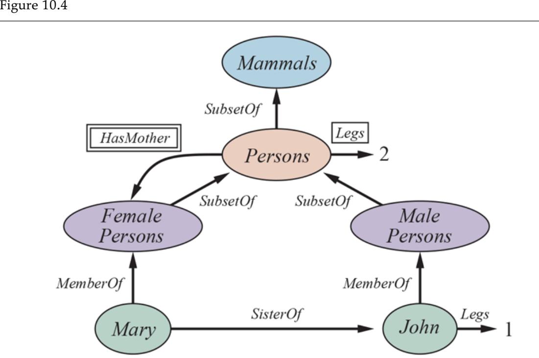
A semantic network with four objects (John, Mary, 1, and 2) and four categories. Relations are denoted by labeled links.

For this reason, we have used a special notation—the double-boxed link—in Figure 10.4 . This link asserts that

\[\forall x \qquad x \in Personons \Rightarrow \left[ \forall \; y \qquad HasMother(x, y) \Rightarrow y \in PemalePersons \right] \dots\]

We might also want to assert that persons have two legs—that is,

\[\forall \, x \qquad x \in Persons \RightarrowLegs(x, 2) \; .\]

As before, we need to be careful not to assert that a category has legs; the single-boxed link in Figure 10.4 is used to assert properties of every member of a category.

The semantic network notation makes it convenient to perform inheritance reasoning of the kind introduced in Section 10.2 . For example, by virtue of being a person, Mary inherits the property of having two legs. Thus, to find out how many legs Mary has, the inheritance algorithm follows the MemberOf link from Mary to the category she belongs to, and then follows SubsetOf links up the hierarchy until it finds a category for which there is a boxed Legs link—in this case, the Persons category. The simplicity and efficiency of this inference mechanism, compared with semidecidable logical theorem proving, has been one of the main attractions of semantic networks.

Inheritance becomes complicated when an object can belong to more than one category or when a category can be a subset of more than one other category; this is called multiple inheritance. In such cases, the inheritance algorithm might find two or more conflicting values answering the query. For this reason, multiple inheritance is banned in some objectoriented programming (OOP) languages, such as Java, that use inheritance in a class hierarchy. It is usually allowed in semantic networks, but we defer discussion of that until Section 10.6 .

Multiple inheritance

The reader might have noticed an obvious drawback of semantic network notation, compared to first-order logic: the fact that links between bubbles represent only binary relations. For example, the sentence Fly(Shankar,NewYork,NewDelhi,Yesterday) cannot be asserted directly in a semantic network. Nonetheless, we can obtain the effect of -ary assertions by reifying the proposition itself as an event belonging to an appropriate event category. Figure 10.5 shows the semantic network structure for this particular event. Notice that the restriction to binary relations forces the creation of a rich ontology of reified concepts.

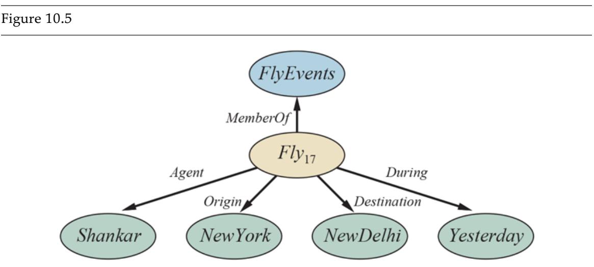
A fragment of a semantic network showing the representation of the logical assertion Fly(Shankar,NewYork,NewDelhi,Yesterday).

Reification of propositions makes it possible to represent every ground, function-free atomic sentence of first-order logic in the semantic network notation. Certain kinds of universally quantified sentences can be asserted using inverse links and the singly boxed and doubly boxed arrows applied to categories, but that still leaves us a long way short of full first-order logic. Negation, disjunction, nested function symbols, and existential quantification are all missing. Now it is possible to extend the notation to make it equivalent to first-order logic as in Peirce’s existential graphs—but doing so negates one of the main advantages of semantic networks, which is the simplicity and transparency of the inference processes. Designers can build a large network and still have a good idea about what queries will be efficient, because (a) it is easy to visualize the steps that the inference procedure will go through and (b) in some cases the query language is so simple that difficult queries cannot be posed.

In cases where the expressive power proves to be too limiting, many semantic network systems provide for procedural attachment to fill in the gaps. Procedural attachment is a technique whereby a query about (or sometimes an assertion of) a certain relation results in a call to a special procedure designed for that relation rather than a general inference algorithm.

Procedural attachment

One of the most important aspects of semantic networks is their ability to represent default values for categories. Examining Figure 10.4 carefully, one notices that John has one leg, despite the fact that he is a person and all persons have two legs. In a strictly logical KB, this would be a contradiction, but in a semantic network, the assertion that all persons have two legs has only default status; that is, a person is assumed to have two legs unless this is contradicted by more specific information. The default semantics is enforced naturally by the inheritance algorithm, because it follows links upwards from the object itself (John in this case) and stops as soon as it finds a value. We say that the default is overridden by the more specific value. Notice that we could also override the default number of legs by creating a category of OneLeggedPersons, a subset of Persons of which John is a member.

Default value

Overriding

We can retain a strictly logical semantics for the network if we say that the Legs assertion for Persons includes an exception for John:

\[\forall \, x \qquad x \in Persons \land x \neq John \Rightarrow Legs(x, 2) \dots\]

For a fixed network, this is semantically adequate but will be much less concise than the network notation itself if there are lots of exceptions. For a network that will be updated with more assertions, however, such an approach fails—we really want to say that any persons as yet unknown with one leg are exceptions too. Section 10.6 goes into more depth on this issue and on default reasoning in general.

10.5.2 Description logics

The syntax of first-order logic is designed to make it easy to say things about objects. Description logics are notations that are designed to make it easier to describe definitions and properties of categories. Description logic systems evolved from semantic networks in response to pressure to formalize what the networks mean while retaining the emphasis on taxonomic structure as an organizing principle.

Description logic

The principal inference tasks for description logics are subsumption (checking if one category is a subset of another by comparing their definitions) and classification (checking whether an object belongs to a category). Some systems also include consistency of a category definition—whether the membership criteria are logically satisfiable.

Subsumption

Classification

Consistency

The CLASSIC language (Borgida et al., 1989) is a typical description logic. The syntax of CLASSIC descriptions is shown in Figure 10.6 . For example, to say that bachelors are unmarried adult males we would write 6

6 Notice that the language does not allow one to simply state that one concept, or category, is a subset of another. This is a deliberate policy: subsumption between categories must be derivable from some aspects of the descriptions of the categories. If not, then something is missing from the descriptions.

Figure 10.6

The syntax of descriptions in a subset of the CLASSIC language.

The equivalent in first-order logic would be

Notice that the description logic has an algebra of operations on predicates, which of course we can’t do in first-order logic. Any description in CLASSIC can be translated into an equivalent first-order sentence, but some descriptions are more straightforward in CLASSIC. For example, to describe the set of men with at least three sons who are all unemployed and married to doctors, and at most two daughters who are all professors in physics or math departments, we would use

We leave it as an exercise to translate this into first-order logic.

Perhaps the most important aspect of description logics is their emphasis on tractability of inference. A problem instance is solved by describing it and then asking if it is subsumed by one of several possible solution categories. In standard first-order logic systems, predicting the solution time is often impossible. It is frequently left to the user to engineer the representation to detour around sets of sentences that seem to be causing the system to take several weeks to solve a problem. The thrust in description logics, on the other hand, is to ensure that subsumption-testing can be solved in time polynomial in the size of the descriptions. 7

7 CLASSIC provides efficient subsumption testing in practice, but the worst-case run time is exponential.

This sounds wonderful in principle, until one realizes that it can only have one of two consequences: either hard problems cannot be stated at all, or they require exponentially large descriptions! However, the tractability results do shed light on what sorts of constructs cause problems and thus help the user to understand how different representations behave. For example, description logics usually lack negation and disjunction. Each forces first-order logical systems to go through a potentially exponential case analysis in order to ensure completeness. CLASSIC allows only a limited form of disjunction in the Fills and OneOf constructs, which permit disjunction over explicitly enumerated individuals but not over descriptions. With disjunctive descriptions, nested definitions can lead easily to an exponential number of alternative routes by which one category can subsume another.

10.6 Reasoning with Default Information

In the preceding section, we saw a simple example of an assertion with default status: people have two legs. This default can be overridden by more specific information, such as that Long John Silver has one leg. We saw that the inheritance mechanism in semantic networks implements the overriding of defaults in a simple and natural way. In this section, we study defaults more generally, with a view toward understanding the semantics of defaults rather than just providing a procedural mechanism.

10.6.1 Circumscription and default logic

We have seen two examples of reasoning processes that violate the monotonicity property of logic that was proved in Chapter 7 . In this chapter we saw that a property inherited by all members of a category in a semantic network could be overridden by more specific information for a subcategory. In Section 9.4.4 , we saw that under the closed-world assumption, if a proposition is not mentioned in then , but . 8

8 Recall that monotonicity requires all entailed sentences to remain entailed after new sentences are added to the KB. That is, if then .

Simple introspection suggests that these failures of monotonicity are widespread in commonsense reasoning. It seems that humans often “jump to conclusions.” For example, when one sees a car parked on the street, one is normally willing to believe that it has four wheels even though only three are visible. Now, probability theory can certainly provide a conclusion that the fourth wheel exists with high probability; yet, for most people, the possibility that the car does not have four wheels will not arise unless some new evidence presents itself. Thus, it seems that the four-wheel conclusion is reached by default, in the absence of any reason to doubt it. If new evidence arrives—for example, if one sees the owner carrying a wheel and notices that the car is jacked up—then the conclusion can be retracted. This kind of reasoning is said to exhibit nonmonotonicity, because the set of beliefs does not grow monotonically over time as new evidence arrives. Nonmonotonic logics have been devised with modified notions of truth and entailment in order to capture such behavior. We will look at two such logics that have been studied extensively: circumscription and default logic.

Nonmonotonicity

Nonmonotonic logic

Circumscription

Circumscription can be seen as a more powerful and precise version of the closed-world assumption. The idea is to specify particular predicates that are assumed to be “as false as possible”—that is, false for every object except those for which they are known to be true. For example, suppose we want to assert the default rule that birds fly. We would introduce a predicate, say , and write

If we say that is to be circumscribed, a circumscriptive reasoner is entitled to assume unless is known to be true. This allows the conclusion Flies(Tweety) to be drawn from the premise Bird(Tweety), but the conclusion no longer holds if is asserted.

Circumscription can be viewed as an example of a model preference logic. In such logics, a sentence is entailed (with default status) if it is true in all preferred models of the KB, as opposed to the requirement of truth in all models in classical logic. For circumscription, one model is preferred to another if it has fewer abnormal objects. Let us see how this idea works in the context of multiple inheritance in semantic networks. The standard example for which multiple inheritance is problematic is called the “Nixon diamond.” It arises from the observation that Richard Nixon was both a Quaker (and hence by default a pacifist) and a Republican (and hence by default not a pacifist). We can write this as follows: 9

9 For the closed-world assumption, one model is preferred to another if it has fewer true atoms—that is, preferred models are minimal models. There is a natural connection between the closed-world assumption and definite-clause KBs, because the fixed point reached

by forward chaining on definite-clause KBs is the unique minimal model. See page 231 for more on this point.

Model preference

If we circumscribe and , there are two preferred models: one in which and Pacifist(Nixon) are true and one in which and are true. Thus, the circumscriptive reasoner remains properly agnostic as to whether Nixon was a pacifist. If we wish, in addition, to assert that religious beliefs take precedence over political beliefs, we can use a formalism called prioritized circumscription to give preference to models where is minimized.

Prioritized circumscription

Default logic is a formalism in which default rules can be written to generate contingent, nonmonotonic conclusions. A default rule looks like this:

Default logic

Default rules

This rule means that if is true, and if is consistent with the knowledge base, then may be concluded by default. In general, a default rule has the form

\[P: J\_1, \dots, J\_n/C\]

where is called the prerequisite, is the conclusion, and are the justifications—if any one of them can be proven false, then the conclusion cannot be drawn. Any variable that appears in or must also appear in . The Nixon-diamond example can be represented in default logic with one fact and two default rules:

To interpret what the default rules mean, we define the notion of an extension of a default theory to be a maximal set of consequences of the theory. That is, an extension consists of the original known facts and a set of conclusions from the default rules, such that no additional conclusions can be drawn from , and the justifications of every default conclusion in are consistent with . As in the case of the preferred models in circumscription, we have two possible extensions for the Nixon diamond: one wherein he is a pacifist and one wherein he is not. Prioritized schemes exist in which some default rules can be given precedence over others, allowing some ambiguities to be resolved.

Extension

Since 1980, when nonmonotonic logics were first proposed, a great deal of progress has been made in understanding their mathematical properties. There are still unresolved questions, however. For example, if “Cars have four wheels” is false, what does it mean to have it in one’s knowledge base? What is a good set of default rules to have? If we cannot decide, for each rule separately, whether it belongs in our knowledge base, then we have a serious problem of nonmodularity. Finally, how can beliefs that have default status be used to make decisions? This is probably the hardest issue for default reasoning.

Decisions often involve tradeoffs, and one therefore needs to compare the strengths of belief in the outcomes of different actions, and the costs of making a wrong decision. In cases where the same kinds of decisions are being made repeatedly, it is possible to interpret default rules as “threshold probability” statements. For example, the default rule “My brakes are always OK” really means “The probability that my brakes are OK, given no other information, is sufficiently high that the optimal decision is for me to drive without checking them.” When the decision context changes—for example, when one is driving a heavily laden truck down a steep mountain road—the default rule suddenly becomes inappropriate, even though there is no new evidence of faulty brakes. These considerations have led researchers to consider how to embed default reasoning within probability theory or utility theory.

10.6.2 Truth maintenance systems

We have seen that many of the inferences drawn by a knowledge representation system will have only default status, rather than being absolutely certain. Inevitably, some of these inferred facts will turn out to be wrong and will have to be retracted in the face of new information. This process is called belief revision. Suppose that a knowledge base contains a sentence —perhaps a default conclusion recorded by a forward-chaining algorithm, or perhaps just an incorrect assertion—and we want to execute TELL( , ). To avoid creating a contradiction, we must first execute RETRACT( , ). This sounds easy enough. Problems arise, however, if any additional sentences were inferred from and asserted in the KB. For example, the implication might have been used to add . The obvious “solution”—retracting all sentences inferred from —fails because such sentences may have other justifications besides . For example, if and are also in the KB, then does not have to be removed after all. Truth maintenance systems, or TMSs, are designed to handle exactly these kinds of complications. 10

10 Belief revision is often contrasted with belief update, which occurs when a knowledge base is revised to reflect a change in the world rather than new information about a fixed world. Belief update combines belief revision with reasoning about time and change; it is also related to the process of filtering described in Chapter 14 .

Belief revision

Truth maintenance system

One simple approach to truth maintenance is to keep track of the order in which sentences are told to the knowledge base by numbering them from to . When the call RETRACT( , ) is made, the system reverts to the state just before was added, thereby removing both and any inferences that were derived from . The sentences through can then be added again. This is simple, and it guarantees that the knowledge base will be consistent, but retracting requires retracting and reasserting sentences as well as undoing and redoing all the inferences drawn from those sentences. For systems to which many facts are being added—such as large commercial databases—this is impractical.

A more efficient approach is the justification-based truth maintenance system, or JTMS. In a JTMS, each sentence in the knowledge base is annotated with a justification consisting of the set of sentences from which it was inferred. For example, if the knowledge base already contains , then TELL will cause to be added with the justification . In general, a sentence can have any number of justifications. Justifications make retraction efficient. Given the call RETRACT , the JTMS will delete exactly those sentences for which is a member of every justification. So, if a sentence had the single justification , it would be removed; if it had the additional justification , it would still be removed; but if it also had the justification , then it would be spared. In this way, the time required for retraction of depends only on the number of sentences derived from rather than on the number of sentences added after .

JTMS

Justification

The JTMS assumes that sentences that are considered once will probably be considered again, so rather than deleting a sentence from the knowledge base entirely when it loses all justifications, we merely mark the sentence as being out of the knowledge base. If a subsequent assertion restores one of the justifications, then we mark the sentence as being back in. In this way, the JTMS retains all the inference chains that it uses and need not rederive sentences when a justification becomes valid again.

In addition to handling the retraction of incorrect information, TMSs can be used to speed up the analysis of multiple hypothetical situations. Suppose, for example, that the Romanian Olympic Committee is choosing sites for the swimming, athletics, and equestrian events at the 2048 Games to be held in Romania. For example, let the first hypothesis be Site(Swimming,Pitesti), Site(Athletics,Bucharest), and (Equestrian,Arad).

A great deal of reasoning must then be done to work out the logistical consequences and hence the desirability of this selection. If we want to consider Site(Athletics,Sibiu) instead, the TMS avoids the need to start again from scratch. Instead, we simply retract Site(Athletics,Bucharest) and assert Site(Athletics,Sibiu) and the TMS takes care of the necessary revisions. Inference chains generated from the choice of Bucharest can be reused with Sibiu, provided that the conclusions are the same.

An assumption-based truth maintenance system, or ATMS, makes this type of contextswitching between hypothetical worlds particularly efficient. In a JTMS, the maintenance of justifications allows you to move quickly from one state to another by making a few retractions and assertions, but at any time only one state is represented. An ATMS represents all the states that have ever been considered at the same time. Whereas a JTMS simply labels each sentence as being in or out, an ATMS keeps track, for each sentence, of which assumptions would cause the sentence to be true. In other words, each sentence has a label that consists of a set of assumption sets. The sentence is true just in those cases in which all the assumptions in one of the assumption sets are true.

ATMS

Explanation

Truth maintenance systems also provide a mechanism for generating explanations. Technically, an explanation of a sentence is a set of sentences such that entails . If the sentences in are already known to be true, then simply provides a sufficient basis for proving that must be the case. But explanations can also include assumptions sentences that are not known to be true, but would suffice to prove if they were true. For example, if your car won’t start, you probably don’t have enough information to definitively prove the reason for the problem. But a reasonable explanation might include the assumption that the battery is dead. This, combined with knowledge of how cars operate, explains the observed nonbehavior. In most cases, we will prefer an explanation that is minimal, meaning that there is no proper subset of that is also an explanation. An ATMS can generate explanations for the “car won’t start” problem by making assumptions (such as “no gas in car” or “battery dead”) in any order we like, even if some assumptions are contradictory. Then we look at the label for the sentence “car won’t start” to read off the sets of assumptions that would justify the sentence.

Assumption

The exact algorithms used to implement truth maintenance systems are a little complicated, and we do not cover them here. The computational complexity of the truth maintenance problem is at least as great as that of propositional inference—that is, NP-hard. Therefore, you should not expect truth maintenance to be a panacea. When used carefully, however, a TMS can provide a substantial increase in the ability of a logical system to handle complex environments and hypotheses.

Summary

By delving into the details of how one represents a variety of knowledge, we hope we have given the reader a sense of how real knowledge bases are constructed and a feeling for the interesting philosophical issues that arise. The major points are as follows:

• Large-scale knowledge representation requires a general-purpose ontology to organize and tie together the various specific domains of knowledge.
• A general-purpose ontology needs to cover a wide variety of knowledge and should be capable, in principle, of handling any domain.
• Building a large, general-purpose ontology is a significant challenge that has yet to be fully realized, although current frameworks seem to be quite robust.
• We presented an upper ontology based on categories and the event calculus. We covered categories, subcategories, parts, structured objects, measurements, substances, events, time and space, change, and beliefs.
• Natural kinds cannot be defined completely in logic, but properties of natural kinds can be represented.
• Actions, events, and time can be represented with the event calculus. Such representations enable an agent to construct sequences of actions and make logical inferences about what will be true when these actions happen.
• Special-purpose representation systems, such as semantic networks and description logics, have been devised to help in organizing a hierarchy of categories. Inheritance is an important form of inference, allowing the properties of objects to be deduced from their membership in categories.
• The closed-world assumption, as implemented in logic programs, provides a simple way to avoid having to specify lots of negative information. It is best interpreted as a default that can be overridden by additional information.
• Nonmonotonic logics, such as circumscription and default logic, are intended to capture default reasoning in general.
• Truth maintenance systems handle knowledge updates and revisions efficiently.
• It is difficult to construct large ontologies by hand; extracting knowledge from text makes the job easier.

Bibliographical and Historical Notes

Briggs (1985) claims that knowledge representation research began with first millennium BCE Indian theorizing about the grammar of Shastric Sanskrit. Western philosophers trace their work on the subject back to c. 300 BCE in Aristotle’s Metaphysics (literally, what comes after the book on physics). The development of technical terminology in any field can be regarded as a form of knowledge representation.

Early discussions of representation in AI tended to focus on ” problem representation” rather than “knowledge representation.” (See, for example, Amarel’s (1968) discussion of the “Missionaries and Cannibals” problem.) In the 1970s, AI emphasized the development of “expert systems” (also called “knowledge-based systems”) that could, if given the appropriate domain knowledge, match or exceed the performance of human experts on narrowly defined tasks. For example, the first expert system, DENDRAL (Feigenbaum et al., 1971; Lindsay et al., 1980), interpreted the output of a mass spectrometer (a type of instrument used to analyze the structure of organic chemical compounds) as accurately as expert chemists. Although the success of DENDRAL was instrumental in convincing the AI research community of the importance of knowledge representation, the representational formalisms used in DENDRAL are highly specific to the domain of chemistry.

Over time, researchers became interested in standardized knowledge representation formalisms and ontologies that could assist in the creation of new expert systems. This brought them into territory previously explored by philosophers of science and of language. The discipline imposed in AI by the need for one’s theories to “work” has led to more rapid and deeper progress than when these problems were the exclusive domain of philosophy (although it has at times also led to the repeated reinvention of the wheel).

But to what extent can we trust expert knowledge? As far back as 1955, Paul Meehl (see also Grove and Meehl, 1996) studied the decision-making processes of trained experts at subjective tasks such as predicting the success of a student in a training program or the recidivism of a criminal. In 19 out of the 20 studies he looked at, Meehl found that simple statistical learning algorithms (such as linear regression or naive Bayes) predict better than the experts. Tetlock (2017) also studies expert knowledge and finds it lacking in difficult cases. The Educational Testing Service has used an automated program to grade millions of

essay questions on the GMAT exam since 1999. The program agrees with human graders 97% of the time, about the same level that two human graders agree (Burstein et al., 2001). (This does not mean the program understands essays, just that it can distinguish good ones from bad ones about as well as human graders can.)

The creation of comprehensive taxonomies or classifications dates back to ancient times. Aristotle (384–322 BCE) strongly emphasized classification and categorization schemes. His Organon, a collection of works on logic assembled by his students after his death, included a treatise called Categories in which he attempted to construct what we would now call an upper ontology. He also introduced the notions of genus and species for lower-level classification. Our present system of biological classification, including the use of “binomial nomenclature” (classification via genus and species in the technical sense), was invented by the Swedish biologist Carolus Linnaeus, or Carl von Linne (1707–1778). The problems associated with natural kinds and inexact category boundaries have been addressed by Wittgenstein (1953), Quine (1953), Lakoff (1987), and Schwartz (1977), among others.

See Chapter 24 for a discussion of deep neural network representations of words and concepts that escape some of the problems of a strict ontology, but also sacrifice some of the precision. We still don’t know the best way to combine the advantages of neural networks and logical semantics for representation.

Interest in larger-scale ontologies is increasing, as documented by the Handbook on Ontologies (Staab, 2004). The OPENCYC project (Lenat and Guha, 1990; Matuszek et al., 2006) has released a 150,000-concept ontology, with an upper ontology similar to the one in Figure 10.1 as well as specific concepts like “OLED Display” and “iPhone,” which is a type of “cellular phone,” which in turn is a type of “consumer electronics,” “phone,” “wireless communication device,” and other concepts. The NEXTKB project extends CYC and other resources including FrameNet and WordNet into a knowledge base with almost 3 million facts, and provides a reasoning engine, FIRE to go with it (Forbus et al., 2010).

The DBPEDIA project extracts structured data from Wikipedia, specifically from Infoboxes: the attribute/value pairs that accompany many Wikipedia articles (Wu and Weld, 2008; Bizer et al., 2007). As of 2015, DBPEDIA contained 400 million facts about 4 million objects in the English version alone; counting all 110 languages yields 1.5 billion facts (Lehmann et al., 2015).

The IEEE working group P1600.1 created SUMO, the Suggested Upper Merged Ontology (Niles and Pease, 2001; Pease and Niles, 2002), with about 1000 terms in the upper ontology and links to over 20,000 domain-specific terms. Stoffel et al., (1997) describe algorithms for efficiently managing a very large ontology. A survey of techniques for extracting knowledge from Web pages is given by Etzioni et al., (2008).

On the Web, representation languages are emerging. RDF (Brickley and Guha, 2004) allows for assertions to be made in the form of relational triples and provides some means for evolving the meaning of names over time. OWL (Smith et al., 2004) is a description logic that supports inferences over these triples. So far, usage seems to be inversely proportional to representational complexity: the traditional HTML and CSS formats account for over 99% of Web content, followed by the simplest representation schemes, such as RDFa (Adida and Birbeck, 2008), and microformats (Khare, 2006; Patel-Schneider, 2014) which use HTML and XHTML markup to add attributes to text on web pages. Usage of sophisticated RDF and OWL ontologies is not yet widespread, and the full vision of the Semantic Web (Berners-Lee et al., 2001) has not been realized. The conferences on Formal Ontology in Information Systems (FOIS) covers both general and domain-specific ontologies.

The taxonomy used in this chapter was developed by the authors and is based in part on their experience in the CYC project and in part on work by Hwang and Schubert (1993) and Davis (1990, 2005). An inspirational discussion of the general project of commonsense knowledge representation appears in Hayes’s (1978, 1985b) “Naive Physics Manifesto.”

Successful deep ontologies within a specific field include the Gene Ontology project (Gene Ontology Consortium, 2008) and the Chemical Markup Language (Murray-Rust et al., 2003). Doubts about the feasibility of a single ontology for all knowledge are expressed by Doctorow (2001), Gruber (2004), Halevy et al. (2009), and Smith (2004).

The event calculus was introduced by Kowalski and Sergot (1986) to handle continuous time, and there have been several variations (Sadri and Kowalski, 1995; Shanahan, 1997) and overviews (Shanahan, 1999; Mueller, 2006). James Allen introduced time intervals for the same reason (Allen, 1984), arguing that intervals were much more natural than situations for reasoning about extended and concurrent events. In van Lambalgen and Hamm (2005) we see how the logic of events maps onto the language we use to talk about events. An alternative to the event and situation calculi is the fluent calculus (Thielscher, 1999), which reifies the facts out of which states are composed.

Peter Ladkin (1986a, 1986b) introduced “concave” time intervals (intervals with gaps essentially, unions of ordinary “convex” time intervals) and applied the techniques of mathematical abstract algebra to time representation. Allen (1991) systematically investigates the wide variety of techniques available for time representation; van Beek and Manchak (1996) analyze algorithms for temporal reasoning. There are significant commonalities between the event-based ontology given in this chapter and an analysis of events due to the philosopher Donald Davidson (1980). The histories in Pat Hayes’s (1985a) ontology of liquids and the chronicles in McDermott’s (1985) theory of plans were also important influences on the field and on this chapter.

The question of the ontological status of substances has a long history. Plato proposed that substances were abstract entities entirely distinct from physical objects; he would say rather than . This leads to a substance hierarchy in which, for example, UnsaltedButter is a more specific substance than Butter. The position adopted in this chapter, in which substances are categories of objects, was championed by Richard Montague (1973). It has also been adopted in the CYC project. Copeland (1993) mounts a serious, but not invincible, attack.

The alternative approach mentioned in the chapter, in which butter is one object consisting of all buttery objects in the universe, was proposed originally by the Polish logician Leśniewski (1916). His mereology (the name is derived from the Greek word for “part”) used the part–whole relation as a substitute for mathematical set theory, with the aim of eliminating abstract entities such as sets. A more readable exposition of these ideas is given by Leonard and Goodman (1940), and Goodman’s The Structure of Appearance (1977) applies the ideas to various problems in knowledge representation.

While some aspects of the mereological approach are awkward—for example, the need for a separate inheritance mechanism based on part–whole relations—the approach gained the support of Quine (1960). Harry Bunt (1985) has provided an extensive analysis of its use in knowledge representation. Casati and Varzi (1999) cover parts, wholes, and a general theory of spatial locations.

There are three main approaches to the study of mental objects. The one taken in this chapter, based on modal logic and possible worlds, is the classical approach from philosophy (Hintikka, 1962; Kripke, 1963; Hughes and Cresswell, 1996). The book Reasoning about Knowledge (Fagin et al., 1995) provides a thorough introduction, and Gordon and Hobbs (2017) provide A Formal Theory of Commonsense Psychology.

The second approach is a first-order theory in which mental objects are fluents. Davis (2005) and Davis and Morgenstern (2005) describe this approach. It relies on the possibleworlds formalism, and builds on work by Robert Moore (1980, 1985).

The third approach is a syntactic theory, in which mental objects are represented by character strings. A string is just a complex term denoting a list of symbols, so CanFly(Clark) can be represented by the list of symbols . The syntactic theory of mental objects was first studied in depth by Kaplan and Montague (1960), who showed that it led to paradoxes if not handled carefully. Ernie Davis (1990) provides an excellent comparison of the syntactic and modal theories of knowledge. Pnueli (1977) describes a temporal logic used to reason about programs, work that won him the Turing Award and which was expanded upon by Vardi (1996). Littman et al. (2017) show that a temporal logic can be a good language for specifying goals to a reinforcement learning robot in a way that is easy for a human to specify, and generalizes well to different environments.

The Greek philosopher Porphyry (c. 234–305 CE), commenting on Aristotle’s Categories, drew what might qualify as the first semantic network. Charles S. Peirce (1909) developed existential graphs as the first semantic network formalism using modern logic. Ross Quillian (1961), driven by an interest in human memory and language processing, initiated work on semantic networks within AI. An influential paper by Marvin Minsky (1975) presented a version of semantic networks called frames; a frame was a representation of an object or category, with attributes and relations to other objects or categories.

The question of semantics arose quite acutely with respect to Quillian’s semantic networks (and those of others who followed his approach), with their ubiquitous and very vague “IS-A links” Bill Woods’s (1975) famous article “What’s In a Link?” drew the attention of AI researchers to the need for precise semantics in knowledge representation formalisms. Ron Brachman (1979) elaborated on this point and proposed solutions. Patrick Hayes’s (1979) “The Logic of Frames” cut even deeper, claiming that “Most of ‘frames’ is just a new syntax

for parts of first-order logic.” Drew McDermott’s (1978b) “Tarskian Semantics, or, No Notation without Denotation!” argued that the model-theoretic approach to semantics used in first-order logic should be applied to all knowledge representation formalisms. This remains a controversial idea; notably, McDermott himself has reversed his position in “A Critique of Pure Reason” (McDermott, 1987). Selman and Levesque (1993) discuss the complexity of inheritance with exceptions, showing that in most formulations it is NPcomplete.

Description logics were developed as a useful subset of first-order logic for which inference is computationally tractable. Hector Levesque and Ron Brachman (1987) showed that certain uses of disjunction and negation were primarily responsible for the intractability of logical inference. This led to a better understanding of the interaction between complexity and expressiveness in reasoning systems. Calvanese et al. (1999) summarize the state of the art, and Baader et al. (2007) present a comprehensive handbook of description logic.

The three main formalisms for dealing with nonmonotonic inference—circumscription (McCarthy, 1980), default logic (Reiter, 1980), and modal nonmonotonic logic (McDermott and Doyle, 1980)—were all introduced in one special issue of the AI Journal. Delgrande and Schaub (2003) discuss the merits of the variants, given 25 years of hindsight. Answer set programming can be seen as an extension of negation as failure or as a refinement of circumscription; the underlying theory of stable model semantics was introduced by Gelfond and Lifschitz, (1988), and the leading answer set programming systems are DLV (Eiter et al. 1998) and SMODELS (Niemelä et al. 2000). Lifschitz (2001) discusses the use of answer set programming for planning. Brewka et al., (1997) give a good overview of the various approaches to nonmonotonic logic. Clark (1978) covers the negation-as-failure approach to logic programming and Clark completion. Lifschitz (2001) discusses the application of answer set programming to planning. A variety of nonmonotonic reasoning systems based on logic programming are documented in the proceedings of the conferences on Logic Programming and Nonmonotonic Reasoning (LPNMR).

The study of truth maintenance systems began with the TMS (Doyle, 1979) and RUP (McAllester, 1980) systems, both of which were essentially JTMSs. Forbus and de Kleer, (1993) explain in depth how TMSs can be used in AI applications. Nayak and Williams, (1997) show how an efficient incremental TMS called an ITMS makes it feasible to plan the operations of a NASA spacecraft in real time.

This chapter could not cover every area of knowledge representation in depth. The three principal topics omitted are the following:

QUALITATIVE PHYSICS: Qualitative physics is a subfield of knowledge representation concerned specifically with constructing a logical, nonnumeric theory of physical objects and processes. The term was coined by Johan de Kleer (1975), although the enterprise could be said to have started in Fahlman’s (1974) BUILD, a sophisticated planner for constructing complex towers of blocks. Fahlman discovered in the process of designing it that most of the effort (80%, by his estimate) went into modeling the physics of the blocks world to calculate the stability of various subassemblies of blocks, rather than into planning per se. He sketches a hypothetical naive-physics-like process to explain why young children can solve BUILD-like problems without access to the high-speed floating-point arithmetic used in BUILD’s physical modeling. Hayes (1985a) uses “histories”—four-dimensional slices of spacetime similar to Davidson’s events—to construct a fairly complex naive physics of liquids. Davis, (2008) gives an update to the ontology of liquids that describes the pouring of liquids into containers.

Qualitative physics

De Kleer and Brown (1985), Ken Forbus (1985), and Benjamin Kuipers, (1985) independently and almost simultaneously developed systems that can reason about a physical system based on qualitative abstractions of the underlying equations. Qualitative physics soon developed to the point where it became possible to analyze an impressive variety of complex physical systems (Yip, 1991). Qualitative techniques have been used to construct novel designs for clocks, windshield wipers, and six-legged walkers (Subramanian and Wang, 1994). The collection Readings in Qualitative Reasoning about Physical Systems (Weld and de Kleer, 1990), an encyclopedia article by Kuipers, (2001), and a handbook article by Davis, (2007) provide good introductions to the field.

SPATIAL REASONING: The reasoning necessary to navigate in the wumpus world is trivial in comparison to the rich spatial structure of the real world. The earliest serious attempt to capture commonsense reasoning about space appears in the work of Ernest Davis (1986,

1990). The region connection calculus of Cohn et al., (1997) supports a form of qualitative spatial reasoning and has led to new kinds of geographical information systems; see also (Davis, 2006). As with qualitative physics, an agent can go a long way, so to speak, without resorting to a full metric representation.

Spatial reasoning

PSYCHOLOGICAL REASONING: Psychological reasoning involves the development of a working psychology for artificial agents to use in reasoning about themselves and other agents. This is often based on so-called folk psychology, the theory that humans in general are believed to use in reasoning about themselves and other humans. When AI researchers provide their artificial agents with psychological theories for reasoning about other agents, the theories are frequently based on the researchers’ description of the logical agents’ own design. Psychological reasoning is currently most useful within the context of natural language understanding, where divining the speaker’s intentions is of paramount importance.

Psychological reasoning

Minker, (2001) collects papers by leading researchers in knowledge representation, summarizing 40 years of work in the field. The proceedings of the international conferences on Principles of Knowledge Representation and Reasoning provide the most up-to-date sources for work in this area. Readings in Knowledge Representation (Brachman and Levesque, 1985) and Formal Theories of the Commonsense World (Hobbs and Moore, 1985) are excellent anthologies on knowledge representation; the former focuses more on historically important papers in representation languages and formalisms, the latter on the accumulation of the knowledge itself. Davis, (1990), Stefik, (1995), and Sowa, (1999) provide textbook introductions to knowledge representation, van Harmelen et al., (2007) contributes a handbook, and Davis and Morgenstern, (2004) edited a special issue of the AI Journal on the topic. Davis, (2017) gives a survey of logic for commonsense reasoning. The biennial conference on Theoretical Aspects of Reasoning About Knowledge (TARK) covers applications of the theory of knowledge in AI, economics, and distributed systems.

Chapter 11 Automated Planning

In which we see how an agent can take advantage of the structure of a problem to efficiently construct complex plans of action.

Planning a course of action is a key requirement for an intelligent agent. The right representation for actions and states and the right algorithms can make this easier. In Section 11.1 we introduce a general factored representation language for planning problems that can naturally and succinctly represent a wide variety of domains, can efficiently scale up to large problems, and does not require ad hoc heuristics for a new domain. Section 11.4 extends the representation language to allow for hierarchical actions, allowing us to tackle more complex problems. We cover efficient algorithms for planning in Section 11.2 , and heuristics for them in Section 11.3 . In Section 11.5 we account for partially observable and nondeterministic domains, and in Section 11.6 we extend the language once again to cover scheduling problems with resource constraints. This gets us closer to planners that are used in the real world for planning and scheduling the operations of spacecraft, factories, and military campaigns. Section 11.7 analyzes the effectiveness of these techniques.

11.1 Definition of Classical Planning

Classical planning is defined as the task of finding a sequence of actions to accomplish a goal in a discrete, deterministic, static, fully observable environment. We have seen two approaches to this task: the problem-solving agent of Chapter 3 and the hybrid propositional logical agent of Chapter 7 . Both share two limitations. First, they both require ad hoc heuristics for each new domain: a heuristic evaluation function for search, and hand-written code for the hybrid wumpus agent. Second, they both need to explicitly represent an exponentially large state space. For example, in the propositional logic model of the wumpus world, the axiom for moving a step forward had to be repeated for all four agent orientations, time steps, and current locations.

Classical planning

In response to these limitations, planning researchers have invested in a factored representation using a family of languages called PDDL, the Planning Domain Definition Language (Ghallab et al. 1998), which allows us to express all actions with a single action schema, and does not need domain-specific knowledge. Basic PDDL can handle classical planning domains, and extensions can handle non-classical domains that are continuous, partially observable, concurrent, and multi-agent. The syntax of PDDL is based on Lisp, but we will translate it into a form that matches the notation used in this book.

PDDL

State

In PDDL, a state is represented as a conjunction of ground atomic fluents. Recall that “ground” means no variables, “fluent” means an aspect of the world that changes over time, and “ground atomic” means there is a single predicate, and if there are any arguments, they must be constants. For example, might represent the state of a hapless agent, and could represent a state in a package delivery problem. PDDL uses database semantics: the closed-world assumption means that any fluents that are not mentioned are false, and the unique names assumption means that and are distinct.

The following fluents are not allowed in a state: (because it has variables), (because it is a negation), and (because it uses a function symbol, Spouse). When convenient, we can think of the conjunction of fluents as a set of fluents.

An action schema represents a family of ground actions. For example, here is an action schema for flying a plane from one location to another:

Action schema

The schema consists of the action name, a list of all the variables used in the schema, a precondition and an effect. The precondition and the effect are each conjunctions of literals (positive or negated atomic sentences). We can choose constants to instantiate the variables, yielding a ground (variable-free) action:

Precondition

Effect

A ground action is applicable in state if entails the precondition of ; that is, if every positive literal in the precondition is in and every negated literal is not.

The result of executing applicable action in state is defined as a state which is represented by the set of fluents formed by starting with , removing the fluents that appear as negative literals in the action’s effects (what we call the delete list or DEL(a)), and adding the fluents that are positive literals in the action’s effects (what we call the add list or ADD(a)):

(11.1)

Delete list

Add list

For example, with the action , we would remove the fluent and add the fluent .

A set of action schemas serves as a definition of a planning domain. A specific problem within the domain is defined with the addition of an initial state and a goal. The initial state is a conjunction of ground fluents (introduced with the keyword Init in Figure 11.1 ). As with all states, the closed-world assumption is used, which means that any atoms that are not mentioned are false. The goal (introduced with Goal) is just like a precondition: a

conjunction of literals (positive or negative) that may contain variables. For example, the goal , refers to any state in which cargo is at SFO but is not, and in which there is a plane at SFO.

11.1.1 Example domain: Air cargo transport

Figure 11.1 shows an air cargo transport problem involving loading and unloading cargo and flying it from place to place. The problem can be defined with three actions: Load, Unload, and Fly. The actions affect two predicates: means that cargo is inside plane , and means that object (either plane or cargo) is at airport . Note that some care must be taken to make sure the At predicates are maintained properly. When a plane flies from one airport to another, all the cargo inside the plane goes with it. In first-order logic it would be easy to quantify over all objects that are inside the plane. But PDDL does not have a universal quantifier, so we need a different solution. The approach we use is to say that a piece of cargo ceases to be At anywhere when it is In a plane; the cargo only becomes At the new airport when it is unloaded. So At really means “available for use at a given location.” The following plan is a solution to the problem:

Figure 11.1

A PDDL description of an air cargo transportation planning problem.

11.1.2 Example domain: The spare tire problem

Consider the problem of changing a flat tire (Figure 11.2 ). The goal is to have a good spare tire properly mounted onto the car’s axle, where the initial state has a flat tire on the axle and a good spare tire in the trunk. To keep it simple, our version of the problem is an abstract one, with no sticky lug nuts or other complications. There are just four actions: removing the spare from the trunk, removing the flat tire from the axle, putting the spare on the axle, and leaving the car unattended overnight. We assume that the car is parked in a particularly bad neighborhood, so that the effect of leaving it overnight is that the tires disappear. is a solution to the problem.

Figure 11.2

The simple spare tire problem.

11.1.3 Example domain: The blocks world

One of the most famous planning domains is the blocks world. This domain consists of a set of cube-shaped blocks sitting on an arbitrarily-large table. The blocks can be stacked, but only one block can fit directly on top of another. A robot arm can pick up a block and move it to another position, either on the table or on top of another block. The arm can pick up only one block at a time, so it cannot pick up a block that has another one on top of it. A typical goal to get block on and block on (see Figure 11.3 ). 1

¹ The blocks world commonly used in planning research is much simpler than SHRDLU’s version (20).

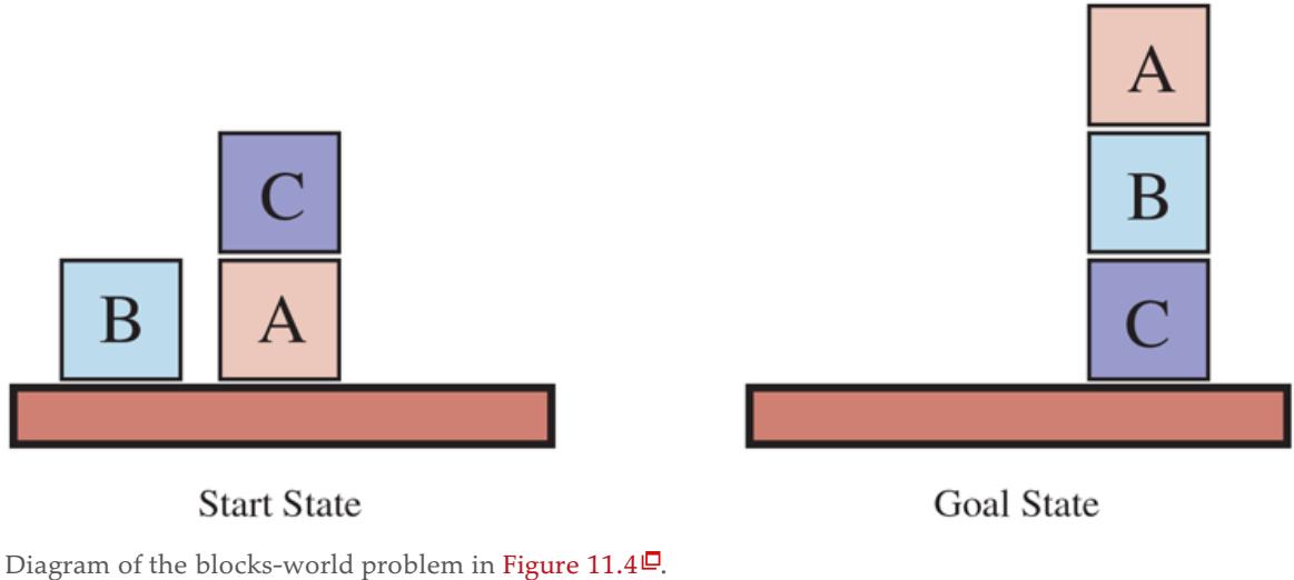
We use to indicate that block is on , where is either another block or the table. The action for moving block from the top of to the top of will be . Now, one of the preconditions on moving is that no other block be on it. In first-order logic, this would be or, alternatively, . Basic PDDL does not allow quantifiers, so instead we introduce a predicate that is true when nothing is on . (The complete problem description is in Figure 11.4 .)

Figure 11.4

A planning problem in the blocks world: building a three-block tower. One solution is the sequence .

The action Move moves a block from to if both and are clear. After the move is made, is still clear but is not. A first attempt at the Move schema is

Unfortunately, this does not maintain Clear properly when or is the table. When is the Table, this action has the effect Clear(Table), but the table should not become clear; and when , it has the precondition Clear(Table), but the table does not have to be clear for us to move a block onto it. To fix this, we do two things. First, we introduce another action to move a block from to the table:

Second, we take the interpretation of to be “there is a clear space on to hold a block.” Under this interpretation, Clear(Table) will always be true. The only problem is that nothing prevents the planner from using instead of . We could live with this problem—it will lead to a larger-than-necessary search space, but will not lead to incorrect answers—or we could introduce the predicate Block and add to the precondition of Move, as shown in Figure 11.4 .

11.2 Algorithms for Classical Planning

The description of a planning problem provides an obvious way to search from the initial state through the space of states, looking for a goal. A nice advantage of the declarative representation of action schemas is that we can also search backward from the goal, looking for the initial state (Figure 11.5 compares forward and backward searches). A third possibility is to translate the problem description into a set of logic sentences, to which we can apply a logical inference algorithm to find a solution.

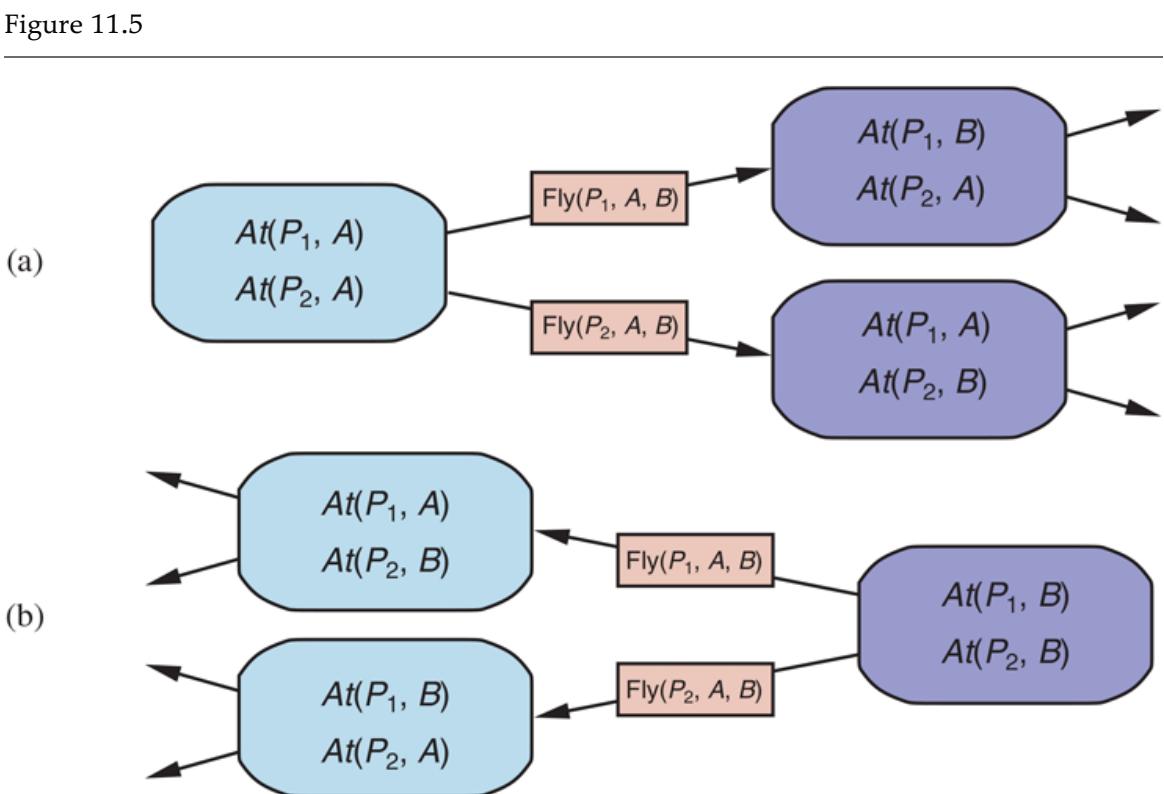
Two approaches to searching for a plan. (a) Forward (progression) search through the space of ground states, starting in the initial state and using the problem’s actions to search forward for a member of the set of goal states. (b) Backward (regression) search through state descriptions, starting at the goal and using the inverse of the actions to search backward for the initial state.

11.2.1 Forward state-space search for planning

We can solve planning problems by applying any of the heuristic search algorithms from Chapter 3 or Chapter 4 . The states in this search state space are ground states, where every fluent is either true or not. The goal is a state that has all the positive fluents in the

problem’s goal and none of the negative fluents. The applicable actions in a state, , are grounded instantiations of the action schemas—that is, actions where the variables have all been replaced by constant values.

To determine the applicable actions we unify the current state against the preconditions of each action schema. For each unification that successfully results in a substitution, we apply the substitution to the action schema to yield a ground action with no variables. (It is a requirement of action schemas that any variable in the effect must also appear in the precondition; that way, we are guaranteed that no variables remain after the substitution.)

Each schema may unify in multiple ways. In the spare tire example (page 346), the Remove action has the precondition , which matches against the initial state in two ways, resulting in the two substitutions and ; applying these substitutions yields two ground actions. If an action has multiple literals in the precondition, then each of them can potentially be matched against the current state in multiple ways.

At first, it seems that the state space might be too big for many problems. Consider an air cargo problem with 10 airports, where each airport initially has 5 planes and 20 pieces of cargo. The goal is to move all the cargo at airport to airport . There is a 41-step solution to the problem: load the 20 pieces of cargo into one of the planes at , fly the plane to , and unload the 20 pieces.

Finding this apparently straightforward solution can be difficult because the average branching factor is huge: each of the 50 planes can fly to 9 other airports, and each of the 200 packages can be either unloaded (if it is loaded) or loaded into any plane at its airport (if it is unloaded). So in any state there is a minimum of 450 actions (when all the packages are at airports with no planes) and a maximum of 10,450 (when all packages and planes are at the same airport). On average, let’s say there are about 2000 possible actions per state, so the search graph up to the depth of the 41-step solution has about nodes.

Clearly, even this relatively small problem instance is hopeless without an accurate heuristic. Although many real-world applications of planning have relied on domain-specific heuristics, it turns out (as we see in Section 11.3 ) that strong domain-independent heuristics can be derived automatically; that is what makes forward search feasible.

11.2.2 Backward search for planning

In backward search (also called regression search) we start at the goal and apply the actions backward until we find a sequence of steps that reaches the initial state. At each step we consider relevant actions (in contrast to forward search, which considers actions that are applicable). This reduces the branching factor significantly, particularly in domains with many possible actions.

Regression search

Relevant action

A relevant action is one with an effect that unifies with one of the goal literals, but with no effect that negates any part of the goal. For example, with the goal , an action with the sole effect Famous would be relevant, but one with the effect is not considered relevant: even though that action might be used at some point in the plan (to establish Famous), it cannot appear at this point in the plan because then Poor would appear in the final state.

What does it mean to apply an action in the backward direction? Given a goal and an action , the regression from over gives us a state description whose positive and negative literals are given by

Regression

That is, the preconditions must have held before, or else the action could not have been executed, but the positive/negative literals that were added/deleted by the action need not have been true before.

These equations are straightforward for ground literals, but some care is required when there are variables in and . For example, suppose the goal is to deliver a specific piece of cargo to SFO: . The Unload action schema has the effect . When we unify that with the goal, we get the substitution ; applying that substitution to the schema gives us a new schema which captures the idea of using any plane that is at SFO:

Here we replaced with a new variable named . This is an instance of standardizing apart variable names so there will be no conflict between different variables that happen to have the same name (see 284). The regressed state description gives us a new goal:

\[g' = In(C\_2, p') \land At(p', SFO) \land Charge(C\_2) \land Plane(p') \land Airort(SFO).\]

As another example, consider the goal of owning a book with a specific ISBN number: . Given a trillion 13-digit ISBNs and the single action schema

a forward search without a heuristic would have to start enumerating the 10 billion ground Buy actions. But with backward search, we would unify the goal with the effect , yielding the substitution . Then we would regress over the action to yield the predecessor state description . This is part of the initial state, so we have a solution and we are done, having considered just one action, not a trillion.

More formally, assume a goal description that contains a goal literal and an action schema . If has an effect literal where and where we define

and if there is no effect in that is the negation of a literal in , then is a relevant action towards .

For most problem domains backward search keeps the branching factor lower than forward search. However, the fact that backward search uses states with variables rather than ground states makes it harder to come up with good heuristics. That is the main reason why the majority of current systems favor forward search.

11.2.3 Planning as Boolean satisfiability

In Section 7.7.4 we showed how some clever axiom-rewriting could turn a wumpus world problem into a propositional logic satisfiability problem that could be handed to an efficient satisfiability solver. SAT-based planners such as SATPLAN operate by translating a PDDL problem description into propositional form. The translation involves a series of steps:

• Propositionalize the actions: for each action schema, form ground propositions by substituting constants for each of the variables. So instead of a single schema, we would have separate action propositions for each combination of cargo, plane, and airport (here written with subscripts), and for each time step (here written as a superscript).
• Add action exclusion axioms saying that no two actions can occur at the same time, e.g. .
• Add precondition axioms: For each ground action , add the axiom , that is, if an action is taken at time , then the preconditions must have been true. For example,

.

• Define the initial state: assert for every fluent in the problem’s initial state, and for every fluent not mentioned in the initial state.
• Propositionalize the goal: the goal becomes a disjunction over all of its ground instances, where variables are replaced by constants. For example, the goal of having block on another block, in a world with objects and , would be replaced by the goal

Add successor-state axioms: For each fluent , add an axiom of the form

where ActionCausesF stands for a disjunction of all the ground actions that add , and ActionCausesNotF stands for a disjunction of all the ground actions that delete .

The resulting translation is typically much larger than the original PDDL, but modern the efficiency of modern SAT solvers often more than makes up for this.

11.2.4 Other classical planning approaches

The three approaches we covered above are not the only ones tried in the 50-year history of automated planning. We briefly describe some others here.

An approach called Graphplan uses a specialized data structure, a planning graph, to encode constraints on how actions are related to their preconditions and effects, and on which things are mutually exclusive.

Planning graph

Situation calculus is a method of describing planning problems in first-order logic. It uses successor-state axioms just as SATPLAN does, but first-order logic allows for more flexibility and more succinct axioms. Overall the approach has contributed to our theoretical understanding of planning, but has not made a big impact in practical applications, perhaps because first-order provers are not as well developed as propositional satisfiability programs.

Situation calculus

It is possible to encode a bounded planning problem (i.e., the problem of finding a plan of length ) as a constraint satisfaction problem (CSP). The encoding is similar to the

encoding to a SAT problem (Section 11.2.3 ), with one important simplification: at each time step we need only a single variable, , whose domain is the set of possible actions. We no longer need one variable for every action, and we don’t need the action exclusion axioms.

All the approaches we have seen so far construct totally ordered plans consisting of strictly linear sequences of actions. But if an air cargo problem has 30 packages being loaded onto one plane and 50 packages being loaded onto another, it seems pointless to decree a specific linear ordering of the 80 load actions.

An alternative called partial-order planning represents a plan as a graph rather than a linear sequence: each action is a node in the graph, and for each precondition of the action there is an edge from another action (or from the initial state) that indicates that the predecessor action establishes the precondition. So we could have a partial-order plan that says that actions Remove(Spare,Trunk) and Remove(Flat,Axle) must come before PutOn(Spare,Axle), but without saying which of the two Remove actions should come first. We search in the space of plans rather than world-states, inserting actions to satisfy conditions.

Partial-order planning

In the 1980s and 1990s, partial-order planning was seen as the best way to handle planning problems with independent subproblems. By 2000, forward-search planners had developed excellent heuristics that allowed them to efficiently discover the independent subproblems that partial-order planning was designed for. Moreover, SATPLAN was able to take advantage of Moore’s law: a propositionalization that was hopelessly large in 1980 now looks tiny, because computers have 10,000 times more memory today. As a result, partialorder planners are not competitive on fully automated classical planning problems.

Nonetheless, partial-order planning remains an important part of the field. For some specific tasks, such as operations scheduling, partial-order planning with domain-specific heuristics

is the technology of choice. Many of these systems use libraries of high-level plans, as described in Section 11.4 .

Partial-order planning is also often used in domains where it is important for humans to understand the plans. For example, operational plans for spacecraft and Mars rovers are generated by partial-order planners and are then checked by human operators before being uploaded to the vehicles for execution. The plan refinement approach makes it easier for the humans to understand what the planning algorithms are doing and to verify that the plans are correct before they are executed.

11.3 Heuristics for Planning

Neither forward nor backward search is efficient without a good heuristic function. Recall from Chapter 3 that a heuristic function estimates the distance from a state to the goal, and that if we can derive an admissible heuristic for this distance—one that does not overestimate—then we can use A* search to find optimal solutions.

By definition, there is no way to analyze an atomic state, and thus it requires some ingenuity by an analyst (usually human) to define good domain-specific heuristics for search problems with atomic states. But planning uses a factored representation for states and actions, which makes it possible to define good domain-independent heuristics.

Recall that an admissible heuristic can be derived by defining a relaxed problem that is easier to solve. The exact cost of a solution to this easier problem then becomes the heuristic for the original problem. A search problem is a graph where the nodes are states and the edges are actions. The problem is to find a path connecting the initial state to a goal state. There are two main ways we can relax this problem to make it easier: by adding more edges to the graph, making it strictly easier to find a path, or by grouping multiple nodes together, forming an abstraction of the state space that has fewer states, and thus is easier to search.

We look first at heuristics that add edges to the graph. Perhaps the simplest is the ignorepreconditions heuristic, which drops all preconditions from actions. Every action becomes applicable in every state, and any single goal fluent can be achieved in one step (if there are any applicable actions—if not, the problem is impossible). This almost implies that the number of steps required to solve the relaxed problem is the number of unsatisfied goals almost but not quite, because (1) some action may achieve multiple goals and (2) some actions may undo the effects of others.

Ignore-preconditions heuristic

For many problems an accurate heuristic is obtained by considering (1) and ignoring (2). First, we relax the actions by removing all preconditions and all effects except those that are literals in the goal. Then, we count the minimum number of actions required such that the union of those actions’ effects satisfies the goal. This is an instance of the set-cover problem. There is one minor irritation: the set-cover problem is NP-hard. Fortunately a simple greedy algorithm is guaranteed to return a set covering whose size is within a factor of of the true minimum covering, where is the number of literals in the goal. Unfortunately, the greedy algorithm loses the guarantee of admissibility.

Set-cover problem

It is also possible to ignore only selected preconditions of actions. Consider the sliding-tile puzzle (8-puzzle or 15-puzzle) from Section 3.2 . We could encode this as a planning problem involving tiles with a single schema Slide:

As we saw in Section 3.6 , if we remove the preconditions then any tile can move in one action to any space and we get the number-of-misplaced-tiles heuristic. If we remove only the precondition then we get the Manhattan-distance heuristic. It is easy to see how these heuristics could be derived automatically from the action schema description. The ease of manipulating the action schemas is the great advantage of the factored representation of planning problems, as compared with the atomic representation of search problems.

Another possibility is the ignore-delete-lists heuristic. Assume for a moment that all goals and preconditions contain only positive literals. We want to create a relaxed version of the original problem that will be easier to solve, and where the length of the solution will serve as a good heuristic. We can do that by removing the delete lists from all actions (i.e., removing all negative literals from effects). That makes it possible to make monotonic progress towards the goal—no action will ever undo progress made by another action. It 2

turns out it is still NP-hard to find the optimal solution to this relaxed problem, but an approximate solution can be found in polynomial time by hill climbing.

2 Many problems are written with this convention. For problems that aren’t, replace every negative literal in a goal or precondition with a new positive literal, , and modify the initial state and the action effects accordingly.

Ignore-delete-lists heuristic

Figure 11.6 diagrams part of the state space for two planning problems using the ignoredelete-lists heuristic. The dots represent states and the edges actions, and the height of each dot above the bottom plane represents the heuristic value. States on the bottom plane are solutions. In both of these problems, there is a wide path to the goal. There are no dead ends, so no need for backtracking; a simple hill-climbing search will easily find a solution to these problems (although it may not be an optimal solution).

Figure 11.6

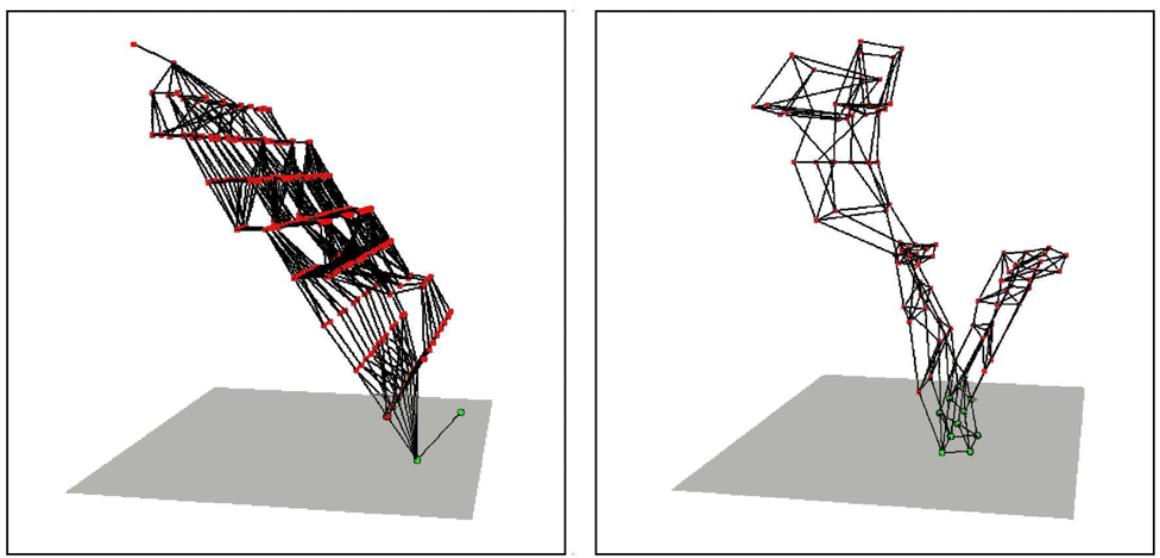
Two state spaces from planning problems with the ignore-delete-lists heuristic. The height above the bottom plane is the heuristic score of a state; states on the bottom plane are goals. There are no local minima, so search for the goal is straightforward. From Hoffmann (2005).

11.3.1 Domain-independent pruning

Factored representations make it obvious that many states are just variants of other states. For example, suppose we have a dozen blocks on a table, and the goal is to have block on top of a three-block tower. The first step in a solution is to place some block on top of block (where , , and are all different). After that, place on top of and we’re done. There are 11 choices for , and given , 10 choices for , and thus 110 states to consider. But all these states are symmetric: choosing one over another makes no difference, and thus a planner should only consider one of them. This is the process of symmetry reduction: we prune out of consideration all symmetric branches of the search tree except for one. For many domains, this makes the difference between intractable and efficient solving.

Symmetry reduction

Another possibility is to do forward pruning, accepting the risk that we might prune away an optimal solution, in order to focus the search on promising branches. We can define a preferred action as follows: First, define a relaxed version of the problem, and solve it to get a relaxed plan. Then a preferred action is either a step of the relaxed plan, or it achieves some precondition of the relaxed plan.

Preferred action

Sometimes it is possible to solve a problem efficiently by recognizing that negative interactions can be ruled out. We say that a problem has serializable subgoals if there exists an order of subgoals such that the planner can achieve them in that order without having to undo any of the previously achieved subgoals. For example, in the blocks world, if the goal is to build a tower (e.g., on , which in turn is on , which in turn is on the Table, as in Figure 11.3 on page 347), then the subgoals are serializable bottom to top: if we first achieve on Table, we will never have to undo it while we are achieving the other subgoals. A planner that uses the bottom-to-top trick can solve any problem in the blocks world without backtracking (although it might not always find the shortest plan). As another

example, if there is a room with light switches, each controlling a separate light, and the goal is to have them all on, then we don’t have to consider permutations of the order; we could arbitrarily restrict ourselves to plans that flip switches in, say, ascending order.

Serializable subgoals

For the Remote Agent planner that commanded NASA’s Deep Space One spacecraft, it was determined that the propositions involved in commanding a spacecraft are serializable. This is perhaps not too surprising, because a spacecraft is designed by its engineers to be as easy as possible to control (subject to other constraints). Taking advantage of the serialized ordering of goals, the Remote Agent planner was able to eliminate most of the search. This meant that it was fast enough to control the spacecraft in real time, something previously considered impossible.

11.3.2 State abstraction in planning

A relaxed problem leaves us with a simplified planning problem just to calculate the value of the heuristic function. Many planning problems have states or more, and relaxing the actions does nothing to reduce the number of states, which means that it may still be expensive to compute the heuristic. Therefore, we now look at relaxations that decrease the number of states by forming a state abstraction—a many-to-one mapping from states in the ground representation of the problem to the abstract representation.

State abstraction

The easiest form of state abstraction is to ignore some fluents. For example, consider an air cargo problem with 10 airports, 50 planes, and 200 pieces of cargo. Each plane can be at one of 10 airports and each package can be either in one of the planes or unloaded at one of the airports. So there are states. Now consider a particular problem in that domain in which it happens that all the packages are at just 5 of the airports, and all

packages at a given airport have the same destination. Then a useful abstraction of the problem is to drop all the At fluents except for the ones involving one plane and one package at each of the 5 airports. Now there are only states. A solution in this abstract state space will be shorter than a solution in the original space (and thus will be an admissible heuristic), and the abstract solution is easy to extend to a solution to the original problem (by adding additional Load and Unload actions).

A key idea in defining heuristics is decomposition: dividing a problem into parts, solving each part independently, and then combining the parts. The subgoal independence assumption is that the cost of solving a conjunction of subgoals is approximated by the sum of the costs of solving each subgoal independently. The subgoal independence assumption can be optimistic or pessimistic. It is optimistic when there are negative interactions between the subplans for each subgoal—for example, when an action in one subplan deletes a goal achieved by another subplan. It is pessimistic, and therefore inadmissible, when subplans contain redundant actions—for instance, two actions that could be replaced by a single action in the merged plan.

Decomposition

Subgoal independence

Suppose the goal is a set of fluents , which we divide into disjoint subsets . We then find optimal plans that solve the respective subgoals. What is an estimate of the cost of the plan for achieving all of ? We can think of each as a heuristic estimate, and we know that if we combine estimates by taking their maximum value, we always get an admissible heuristic. So is admissible, and sometimes it is exactly correct: it could be that serendipitously achieves all the . But usually the estimate is too low. Could we sum the costs instead? For many problems that is a reasonable estimate, but it is not admissible. The best case is when and are independent, in the

sense that plans for one cannot reduce the cost of plans for the other. In that case, the estimate is admissible, and more accurate than the max estimate.

It is clear that there is great potential for cutting down the search space by forming abstractions. The trick is choosing the right abstractions and using them in a way that makes the total cost—defining an abstraction, doing an abstract search, and mapping the abstraction back to the original problem—less than the cost of solving the original problem. The techniques of pattern databases from Section 3.6.3 can be useful, because the cost of creating the pattern database can be amortized over multiple problem instances.

A system that makes use of effective heuristics is FF, or FASTFORWARD (Hoffmann, 2005), a forward state-space searcher that uses the ignore-delete-lists heuristic, estimating the heuristic with the help of a planning graph. FF then uses hill climbing search (modified to keep track of the plan) with the heuristic to find a solution. FF’s hill climbing algorithm is nonstandard: it avoids local maxima by running a breadth-first search from the current state until a better one is found. If this fails, FF switches to a greedy best-first search instead.

11.4 Hierarchical Planning

The problem-solving and planning methods of the preceding chapters all operate with a fixed set of atomic actions. Actions can be strung together, and state-of-the-art algorithms can generate solutions containing thousands of actions. That’s fine if we are planning a vacation and the actions are at the level of “fly from San Francisco to Honolulu,” but at the motor-control level of “bend the left knee by 5 degrees” we would need to string together millions or billions of actions, not thousands.

Bridging this gap requires planning at higher levels of abstraction. A high-level plan for a Hawaii vacation might be “Go to San Francisco airport; take flight HA 11 to Honolulu; do vacation stuff for two weeks; take HA 12 back to San Francisco; go home.” Given such a plan, the action “Go to San Francisco airport” can be viewed as a planning task in itself, with a solution such as “Choose a ride-hailing service; order a car; ride to airport.” Each of these actions, in turn, can be decomposed further, until we reach the low-level motor control actions like a button-press.

In this example, planning and acting are interleaved; for example, one would defer the problem of planning the walk from the curb to the gate until after being dropped off. Thus, that particular action will remain at an abstract level prior to the execution phase. We defer discussion of this topic until Section 11.5 . Here, we concentrate on the idea of hierarchical decomposition, an idea that pervades almost all attempts to manage complexity. For example, complex software is created from a hierarchy of subroutines and classes; armies, governments and corporations have organizational hierarchies. The key benefit of hierarchical structure is that at each level of the hierarchy, a computational task, military mission, or administrative function is reduced to a small number of activities at the next lower level, so the computational cost of finding the correct way to arrange those activities for the current problem is small.

Hierarchical decomposition

11.4.1 High-level actions

The basic formalism we adopt to understand hierarchical decomposition comes from the area of hierarchical task networks or HTN planning. For now we assume full observability and determinism and a set of actions, now called primitive actions, with standard precondition–effect schemas. The key additional concept is the high-level action or HLA for example, the action “Go to San Francisco airport.” Each HLA has one or more possible refinements, into a sequence of actions, each of which may be an HLA or a primitive action. For example, the action “Go to San Francisco airport,” represented formally as Go(Home,SFO), might have two possible refinements, as shown in Figure 11.7 . The same figure shows a recursive refinement for navigation in the vacuum world: to get to a destination, take a step, and then go to the destination.

Figure 11.7

Definitions of possible refinements for two high-level actions: going to San Francisco airport and navigating in the vacuum world. In the latter case, note the recursive nature of the refinements and the use of preconditions.

Hierarchical task network

Primitive action

High-level action

Refinement

These examples show that high-level actions and their refinements embody knowledge about how to do things. For instance, the refinements for Go(Home,SFO) say that to get to the airport you can drive or take a ride-hailing service; buying milk, sitting down, and moving the knight to e4 are not to be considered.

An HLA refinement that contains only primitive actions is called an implementation of the HLA. In a grid world, the sequences [Right,Right,Down] and [Down,Right,Right] both implement the HLA . An implementation of a high-level plan (a sequence of HLAs) is the concatenation of implementations of each HLA in the sequence. Given the precondition–effect definitions of each primitive action, it is straightforward to determine whether any given implementation of a high-level plan achieves the goal.

Implementation

We can say, then, that a high-level plan achieves the goal from a given state if at least one of its implementations achieves the goal from that state. The “at least one” in this definition is crucial —not all implementations need to achieve the goal, because the agent gets to decide which implementation it will execute. Thus, the set of possible implementations in HTN planning —each of which may have a different outcome—is not the same as the set of possible

outcomes in nondeterministic planning. There, we required that a plan work for all outcomes because the agent doesn’t get to choose the outcome; nature does.

The simplest case is an HLA that has exactly one implementation. In that case, we can compute the preconditions and effects of the HLA from those of the implementation (see Exercise 11.HLAU) and then treat the HLA exactly as if it were a primitive action itself. It can be shown that the right collection of HLAs can result in the time complexity of blind search dropping from exponential in the solution depth to linear in the solution depth, although devising such a collection of HLAs may be a nontrivial task in itself. When HLAs have multiple possible implementations, there are two options: one is to search among the implementations for one that works, as in Section 11.4.2 ; the other is to reason directly about the HLAs—despite the multiplicity of implementations—as explained in Section 11.4.3 . The latter method enables the derivation of provably correct abstract plans, without the need to consider their implementations.

11.4.2 Searching for primitive solutions

HTN planning is often formulated with a single “top level” action called Act, where the aim is to find an implementation of Act that achieves the goal. This approach is entirely general. For example, classical planning problems can be defined as follows: for each primitive action , provide one refinement of Act with steps . That creates a recursive definition of Act that lets us add actions. But we need some way to stop the recursion; we do that by providing one more refinement for Act, one with an empty list of steps and with a precondition equal to the goal of the problem. This says that if the goal is already achieved, then the right implementation is to do nothing.

The approach leads to a simple algorithm: repeatedly choose an HLA in the current plan and replace it with one of its refinements, until the plan achieves the goal. One possible implementation based on breadth-first tree search is shown in Figure 11.8 . Plans are considered in order of depth of nesting of the refinements, rather than number of primitive steps. It is straightforward to design a graph-search version of the algorithm as well as depth-first and iterative deepening versions.

A breadth-first implementation of hierarchical forward planning search. The initial plan supplied to the algorithm is . The REFINEMENTS function returns a set of action sequences, one for each refinement of the HLA whose preconditions are satisfied by the specified state, outcome.

In essence, this form of hierarchical search explores the space of sequences that conform to the knowledge contained in the HLA library about how things are to be done. A great deal of knowledge can be encoded, not just in the action sequences specified in each refinement but also in the preconditions for the refinements. For some domains, HTN planners have been able to generate huge plans with very little search. For example, O-PLAN (Bell and Tate, 1985), which combines HTN planning with scheduling, has been used to develop production plans for Hitachi. A typical problem involves a product line of 350 different products, 35 assembly machines, and over 2000 different operations. The planner generates a 30-day schedule with three 8-hour shifts a day, involving tens of millions of steps. Another important aspect of HTN plans is that they are, by definition, hierarchically structured; usually this makes them easy for humans to understand.

The computational benefits of hierarchical search can be seen by examining an idealized case. Suppose that a planning problem has a solution with primitive actions. For a nonhierarchical, forward state-space planner with allowable actions at each state, the cost is , as explained in Chapter 3 . For an HTN planner, let us suppose a very regular refinement structure: each nonprimitive action has possible refinements, each into actions at the next lower level. We want to know how many different refinement trees there are with this structure. Now, if there are actions at the primitive level, then the number of levels below the root is , so the number of internal refinement nodes is . Each internal node has possible refinements, so possible decomposition trees could be constructed.

Examining this formula, we see that keeping small and large can result in huge savings: we are taking the th root of the nonhierarchical cost, if and are comparable. Small and large means a library of HLAs with a small number of refinements each yielding a long action sequence. This is not always possible: long action sequences that are usable across a wide range of problems are extremely rare.

The key to HTN planning is a plan library containing known methods for implementing complex, high-level actions. One way to construct the library is to learn the methods from problem-solving experience. After the excruciating experience of constructing a plan from scratch, the agent can save the plan in the library as a method for implementing the highlevel action defined by the task. In this way, the agent can become more and more competent over time as new methods are built on top of old methods. One important aspect of this learning process is the ability to generalize the methods that are constructed, eliminating detail that is specific to the problem instance (e.g., the name of the builder or the address of the plot of land) and keeping just the key elements of the plan. It seems to us inconceivable that humans could be as competent as they are without some such mechanism.

11.4.3 Searching for abstract solutions

The hierarchical search algorithm in the preceding section refines HLAs all the way to primitive action sequences to determine if a plan is workable. This contradicts common sense: one should be able to determine that the two-HLA high-level plan

gets one to the airport without having to determine a precise route, choice of parking spot, and so on. The solution is to write precondition–effect descriptions of the HLAs, just as we do for primitive actions. From the descriptions, it ought to be easy to prove that the highlevel plan achieves the goal. This is the holy grail, so to speak, of hierarchical planning, because if we derive a high-level plan that provably achieves the goal, working in a small search space of high-level actions, then we can commit to that plan and work on the problem of refining each step of the plan. This gives us the exponential reduction we seek.

For this to work, it has to be the case that every high-level plan that “claims” to achieve the goal (by virtue of the descriptions of its steps) does in fact achieve the goal in the sense

defined earlier: it must have at least one implementation that does achieve the goal. This property has been called the downward refinement property for HLA descriptions.

Downward refinement property

Writing HLA descriptions that satisfy the downward refinement property is, in principle, easy: as long as the descriptions are true, then any high-level plan that claims to achieve the goal must in fact do so—otherwise, the descriptions are making some false claim about what the HLAs do. We have already seen how to write true descriptions for HLAs that have exactly one implementation (Exercise 11.HLAU); a problem arises when the HLA has multiple implementations. How can we describe the effects of an action that can be implemented in many different ways?

One safe answer (at least for problems where all preconditions and goals are positive) is to include only the positive effects that are achieved by every implementation of the HLA and the negative effects of any implementation. Then the downward refinement property would be satisfied. Unfortunately, this semantics for HLAs is much too conservative.

Consider again the HLA Go(Home,SFO), which has two refinements, and suppose, for the sake of argument, a simple world in which one can always drive to the airport and park, but taking a taxi requires Cash as a precondition. In that case, Go(Home,SFO) doesn’t always get you to the airport. In particular, it fails if Cash is false, and so we cannot assert At(Agent,SFO) as an effect of the HLA. This makes no sense, however; if the agent didn’t have Cash, it would drive itself. Requiring that an effect hold for every implementation is equivalent to assuming that someone else—an adversary—will choose the implementation. It treats the HLA’s multiple outcomes exactly as if the HLA were a nondeterministic action, as in Section 4.3 . For our case, the agent itself will choose the implementation.

The programming languages community has coined the term demonic nondeterminism for the case where an adversary makes the choices, contrasting this with angelic nondeterminism, where the agent itself makes the choices. We borrow this term to define angelic semantics for HLA descriptions. The basic concept required for understanding

angelic semantics is the reachable set of an HLA: given a state , the reachable set for an HLA , written as , is the set of states reachable by any of the HLA’s implementations.

Demonic nondeterminism

Angelic nondeterminism

Angelic semantics

Reachable set

The key idea is that the agent can choose which element of the reachable set it ends up in when it executes the HLA; thus, an HLA with multiple refinements is more “powerful” than the same HLA with fewer refinements. We can also define the reachable set of a sequence of HLAs. For example, the reachable set of a sequence is the union of all the reachable sets obtained by applying in each state in the reachable set of :

Given these definitions, a high-level plan—a sequence of HLAs—achieves the goal if its reachable set intersects the set of goal states. (Compare this to the much stronger condition for demonic semantics, where every member of the reachable set has to be a goal state.) Conversely, if the reachable set doesn’t intersect the goal, then the plan definitely doesn’t work. Figure 11.9 illustrates these ideas.

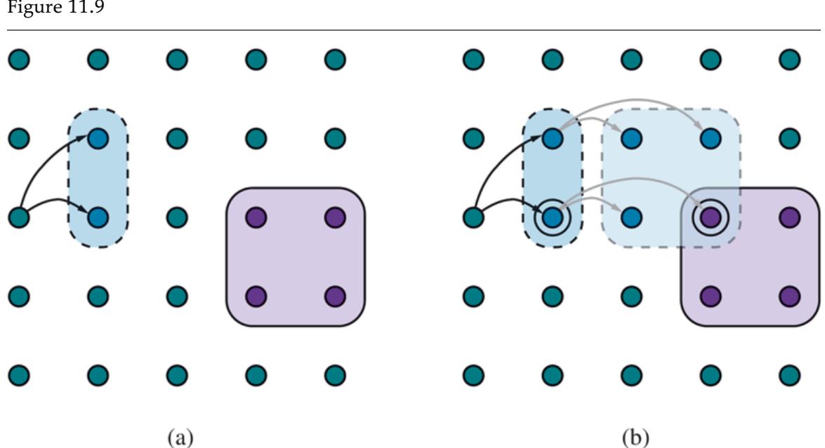
Schematic examples of reachable sets. The set of goal states is shaded in purple. Black and gray arrows indicate possible implementations of and , respectively. (a) The reachable set of an HLA in a state . (b) The reachable set for the sequence . Because this intersects the goal set, the sequence achieves the goal.

The notion of reachable sets yields a straightforward algorithm: search among high-level plans, looking for one whose reachable set intersects the goal; once that happens, the algorithm can commit to that abstract plan, knowing that it works, and focus on refining the plan further. We will return to the algorithmic issues later; for now consider how the effects of an HLA—the reachable set for each possible initial state—are represented. A primitive action can set a fluent to true or false or leave it unchanged. (With conditional effects (see Section 11.5.1 ) there is a fourth possibility: flipping a variable to its opposite.)

An HLA under angelic semantics can do more: it can control the value of a fluent, setting it to true or false depending on which implementation is chosen. That means that an HLA can have nine different effects on a fluent: if the variable starts out true, it can always keep it true, always make it false, or have a choice; if the fluent starts out false, it can always keep it false, always make it true, or have a choice; and the three choices for both cases can be combined arbitrarily, making nine.

Notationally, this is a bit challenging. We’ll use the language of add lists and delete lists (rather than true/false fluents) along with the symbol to mean “possibly, if the agent so chooses.” Thus, the effect means “possibly add ,” that is, either leave unchanged or make it true. Similarly, means “possibly delete” and means “possibly add or delete .” For example, the HLA Go(Home,SFO), with the two refinements shown in Figure 11.7 , possibly deletes Cash (if the agent decides to take a taxi), so it should have the . Thus, we see that the descriptions of HLAs are derivable from the descriptions of their refinements. Now, suppose we have the following schemas for the HLAs and :

\[\begin{aligned} &\mathcal{A}action\left(h\_1, \mathcal{P}\_{\textit{RECON}}; \neg A, \mathcal{E}\_{\textit{FFECT}}; A \wedge \widetilde{-}B\right), \\ &\mathcal{A}action\left(h\_2, \mathcal{P}\_{\textit{RECON}}; \neg B, \mathcal{E}\_{\textit{FFECT}}; \widetilde{+}A \wedge \widetilde{\pm}C\right). \end{aligned}\]

That is, adds and possibly deletes , while possibly adds and has full control over . Now, if only is true in the initial state and the goal is then the sequence achieves the goal: we choose an implementation of that makes false, then choose an implementation of that leaves true and makes true.

The preceding discussion assumes that the effects of an HLA—the reachable set for any given initial state—can be described exactly by describing the effect on each fluent. It would be nice if this were always true, but in many cases we can only approximate the effects because an HLA may have infinitely many implementations and may produce arbitrarily wiggly reachable sets—rather like the wiggly-belief-state problem illustrated in Figure 7.21 on 243. For example, we said that Go(Home,SFO) possibly deletes Cash; it also possibly adds At(Car,SFOLongTermParking); but it cannot do both—in fact, it must do exactly one. As with belief states, we may need to write approximate descriptions. We will use two kinds of approximation: an optimistic description of an HLA may overstate the reachable set, while a pessimistic description may understate the reachable set. Thus, we have

\[\text{REACH}^{-}(s,h) \subseteq \text{REACH}(s,h) \subseteq \text{REACH}^{+}(s,h) \text{ .}\]

Optimistic description

Pessimistic description

For example, an optimistic description of Go(Home,SFO) says that it possibly deletes Cash and possibly adds At(Car,SFOLongTermParking). Another good example arises in the 8 puzzle, half of whose states are unreachable from any given state (see Exercise 11.PART): the optimistic description of Act might well include the whole state space, since the exact reachable set is quite wiggly.

With approximate descriptions, the test for whether a plan achieves the goal needs to be modified slightly. If the optimistic reachable set for the plan doesn’t intersect the goal, then the plan doesn’t work; if the pessimistic reachable set intersects the goal, then the plan does work (Figure 11.10(a) ). With exact descriptions, a plan either works or it doesn’t, but with approximate descriptions, there is a middle ground: if the optimistic set intersects the goal but the pessimistic set doesn’t, then we cannot tell if the plan works (Figure 11.10(b) ). When this circumstance arises, the uncertainty can be resolved by refining the plan. This is a very common situation in human reasoning. For example, in planning the aforementioned two-week Hawaii vacation, one might propose to spend two days on each of seven islands. Prudence would indicate that this ambitious plan needs to be refined by adding details of inter-island transportation.

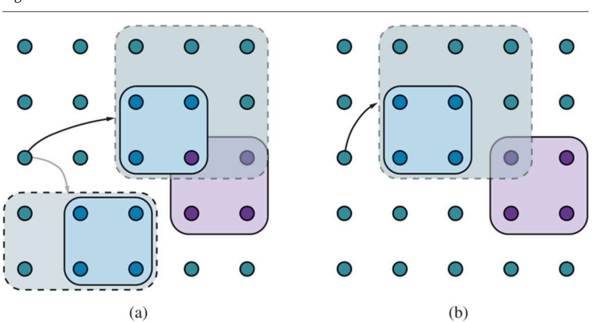
Figure 11.10

Goal achievement for high-level plans with approximate descriptions. The set of goal states is shaded in purple. For each plan, the pessimistic (solid lines, light blue) and optimistic (dashed lines, light green) reachable sets are shown. (a) The plan indicated by the black arrow definitely achieves the goal, while the plan indicated by the gray arrow definitely doesn’t. (b) A plan that possibly achieves the goal (the optimistic reachable set intersects the goal) but does not necessarily achieve the goal (the pessimistic

reachable set does not intersect the goal). The plan would need to be refined further to determine if it really does achieve the goal.

An algorithm for hierarchical planning with approximate angelic descriptions is shown in Figure 11.11 . For simplicity, we have kept to the same overall scheme used previously in Figure 11.8 , that is, a breadth-first search in the space of refinements. As just explained, the algorithm can detect plans that will and won’t work by checking the intersections of the optimistic and pessimistic reachable sets with the goal. (The details of how to compute the reachable sets of a plan, given approximate descriptions of each step, are covered in Exercise 11.HLAP.)

Figure 11.11

A hierarchical planning algorithm that uses angelic semantics to identify and commit to high-level plans that work while avoiding high-level plans that don’t. The predicate MAKING-PROGRESS checks to make sure that we aren’t stuck in an infinite regression of refinements. At top level, call ANGELIC-SEARCH with [Act] as the initialPlan.

When a workable abstract plan is found, the algorithm decomposes the original problem into subproblems, one for each step of the plan. The initial state and goal for each subproblem are obtained by regressing a guaranteed-reachable goal state through the action schemas for each step of the plan. (See Section 11.2.2 for a discussion of how regression works.) Figure 11.9(b) illustrates the basic idea: the right-hand circled state is the guaranteed-reachable goal state, and the left-hand circled state is the intermediate goal obtained by regressing the goal through the final action.

The ability to commit to or reject high-level plans can give ANGELIC-SEARCH a significant computational advantage over HIERARCHICAL-SEARCH, which in turn may have a large advantage over plain old BREADTH-FIRST-SEARCH. Consider, for example, cleaning up a large vacuum world consisting of an arrangement of rooms connected by narrow corridors, where each room is a rectangle of squares. It makes sense to have an HLA for Navigate (as shown in Figure 11.7 ) and one for CleanWholeRoom. (Cleaning the room could be implemented with the repeated application of another HLA to clean each row.) Since there are five primitive actions, the cost for BREADTH-FIRST-SEARCH grows as , where is the length of the shortest solution (roughly twice the total number of squares); the algorithm cannot manage even two rooms. HIERARCHICAL-SEARCH is more efficient, but still suffers from exponential growth because it tries all ways of cleaning that are consistent with the hierarchy. ANGELIC-SEARCH scales approximately linearly in the number of squares—it commits to a good high-level sequence of room-cleaning and navigation steps and prunes away the other options.

Cleaning a set of rooms by cleaning each room in turn is hardly rocket science: it is easy for humans because of the hierarchical structure of the task. When we consider how difficult humans find it to solve small puzzles such as the 8-puzzle, it seems likely that the human capacity for solving complex problems derives not from considering combinatorics, but rather from skill in abstracting and decomposing problems to eliminate combinatorics.

The angelic approach can be extended to find least-cost solutions by generalizing the notion of reachable set. Instead of a state being reachable or not, each state will have a cost for the most efficient way to get there. (The cost is infinite for unreachable states.) The optimistic and pessimistic descriptions bound these costs. In this way, angelic search can find provably optimal abstract plans without having to consider their implementations. The same

approach can be used to obtain effective hierarchical look-ahead algorithms for online search, in the style of LRTA* (page 140).

Hierarchical look-ahead

In some ways, such algorithms mirror aspects of human deliberation in tasks such as planning a vacation to Hawaii—consideration of alternatives is done initially at an abstract level over long time scales; some parts of the plan are left quite abstract until execution time, such as how to spend two lazy days on Moloka’i, while others parts are planned in detail, such as the flights to be taken and lodging to be reserved—without these latter refinements, there is no guarantee that the plan would be feasible.

11.5 Planning and Acting in Nondeterministic Domains

In this section we extend planning to handle partially observable, nondeterministic, and unknown environments. The basic concepts mirror those in Chapter 4 , but there are differences arising from the use of factored representations rather than atomic representations. This affects the way we represent the agent’s capability for action and observation and the way we represent belief states—the sets of possible physical states the agent might be in—for partially observable environments. We can also take advantage of many of the domain-independent methods given in Section 11.3 for calculating search heuristics.

We will cover sensorless planning (also known as conformant planning) for environments with no observations; contingency planning for partially observable and nondeterministic environments; and online planning and replanning for unknown environments. This will allow us to tackle sizable real-world problems.

Consider this problem: given a chair and a table, the goal is to have them match—have the same color. In the initial state we have two cans of paint, but the colors of the paint and the furniture are unknown. Only the table is initially in the agent’s field of view:

There are two actions: removing the lid from a paint can and painting an object using the paint from an open can.

The action schemas are straightforward, with one exception: preconditions and effects now may contain variables that are not part of the action’s variable list. That is, does not mention the variable , representing the color of the paint in the can. In the fully observable case, this is not allowed—we would have to name the action . But in the partially observable case, we might or might not know what color is in the can.

To solve a partially observable problem, the agent will have to reason about the percepts it will obtain when it is executing the plan. The percept will be supplied by the agent’s sensors when it is actually acting, but when it is planning it will need a model of its sensors. In Chapter 4 , this model was given by a function, . For planning, we augment PDDL with a new type of schema, the percept schema:

Percept schema

The first schema says that whenever an object is in view, the agent will perceive the color of the object (that is, for the object , the agent will learn the truth value of for all ). The second schema says that if an open can is in view, then the agent perceives the color of the paint in the can. Because there are no exogenous events in this world, the color of an object will remain the same, even if it is not being perceived, until the agent performs an action to change the object’s color. Of course, the agent will need an action that causes objects (one at a time) to come into view:

For a fully observable environment, we would have a Percept schema with no preconditions for each fluent. A sensorless agent, on the other hand, has no Percept schemas at all. Note that even a sensorless agent can solve the painting problem. One solution is to open any can of paint and apply it to both chair and table, thus coercing them to be the same color (even though the agent doesn’t know what the color is).

A contingent planning agent with sensors can generate a better plan. First, look at the table and chair to obtain their colors; if they are already the same then the plan is done. If not, look at the paint cans; if the paint in a can is the same color as one piece of furniture, then apply that paint to the other piece. Otherwise, paint both pieces with any color.

Finally, an online planning agent might generate a contingent plan with fewer branches at first—perhaps ignoring the possibility that no cans match any of the furniture—and deal with problems when they arise by replanning. It could also deal with incorrectness of its action schemas. Whereas a contingent planner simply assumes that the effects of an action always succeed—that painting the chair does the job—a replanning agent would check the result and make an additional plan to fix any unexpected failure, such as an unpainted area or the original color showing through.

In the real world, agents use a combination of approaches. Car manufacturers sell spare tires and air bags, which are physical embodiments of contingent plan branches designed to handle punctures or crashes. On the other hand, most car drivers never consider these possibilities; when a problem arises they respond as replanning agents. In general, agents plan only for contingencies that have important consequences and a nonnegligible chance of happening. Thus, a car driver contemplating a trip across the Sahara desert should make explicit contingency plans for breakdowns, whereas a trip to the supermarket requires less advance planning. We next look at each of the three approaches in more detail.

11.5.1 Sensorless planning

Section 4.4.1 (page 126) introduced the basic idea of searching in belief-state space to find a solution for sensorless problems. Conversion of a sensorless planning problem to a beliefstate planning problem works much the same way as it did in Section 4.4.1 ; the main differences are that the underlying physical transition model is represented by a collection of action schemas, and the belief state can be represented by a logical formula instead of by an explicitly enumerated set of states. We assume that the underlying planning problem is deterministic.

The initial belief state for the sensorless painting problem can ignore InView fluents because the agent has no sensors. Furthermore, we take as given the unchanging facts because these hold in every belief state. The agent doesn’t know the colors of the cans or the objects, or whether the cans are open or closed, but it does know that objects and cans have colors:

. After Skolemizing (see Section 9.5.1 ), we obtain the initial belief state:

\[b\_0 = Coror(x, C(x)).\]

In classical planning, where the closed-world assumption is made, we would assume that any fluent not mentioned in a state is false, but in sensorless (and partially observable) planning we have to switch to an open-world assumption in which states contain both positive and negative fluents, and if a fluent does not appear, its value is unknown. Thus, the belief state corresponds exactly to the set of possible worlds that satisfy the formula. Given this initial belief state, the following action sequence is a solution:

\[(RemoveList(Can\_1), Point(Chain, Can\_1), Point(Table,Can\_1)).\]

We now show how to progress the belief state through the action sequence to show that the final belief state satisfies the goal.

First, note that in a given belief state , the agent can consider any action whose preconditions are satisfied by . (The other actions cannot be used because the transition model doesn’t define the effects of actions whose preconditions might be unsatisfied.) According to Equation (4.4) (page 127), the general formula for updating the belief state given an applicable action in a deterministic world is as follows:

\[b' = \text{Resur} \text{tr}(b, a) = \left\{ s' : s' = \text{Resur} \text{tr}\_P(s, a) \text{ and } s \in b \right\}\]

where defines the physical transition model. For the time being, we assume that the initial belief state is always a conjunction of literals, that is, a 1-CNF formula. To construct the new belief state , we must consider what happens to each literal in each physical state in when action is applied. For literals whose truth value is already known in , the truth value in is computed from the current value and the add list and delete list

of the action. (For example, if is in the delete list of the action, then is added to .) What about a literal whose truth value is unknown in ? There are three cases:

• 1. If the action adds , then will be true in regardless of its initial value.
• 2. If the action deletes , then will be false in regardless of its initial value.
• 3. If the action does not affect , then will retain its initial value (which is unknown) and will not appear in .

Hence, we see that the calculation of is almost identical to the observable case, which was specified by Equation (11.1) on page 345:

\[b' = \operatorname{Resur}(b, a) = (b - \operatorname{Den}(a)) \cup \operatorname{App}(a) \text{ .}\]

We cannot quite use the set semantics because (1) we must make sure that does not contain both and , and (2) atoms may contain unbound variables. But it is still the case that is computed by starting with , setting any atom that appears in to false, and setting any atom that appears in to true. For example, if we apply to the initial belief state , we get

\[b\_1 = Color(x, C(x)) \land Open(Can\_1).\]

When we apply the action , the precondition is satisfied by the literal with binding and the new belief state is

\[b\_2 = Color(x, C(x)) \land Open(Can\_1) \land Color(Chain, C(Can\_1)).\]

Finally, we apply the action to obtain

\[\begin{aligned} b\_3 &= Color\left(x, C\left(x\right)\right) \land Open\left(Can\_1\right) \land Color\left(Chain, C\left(Can\_1\right)\right) \\ &\land Color\left(Table, C\left(Can\_1\right)\right). \end{aligned}\]

The final belief state satisfies the goal, , with the variable bound to .

The preceding analysis of the update rule has shown a very important fact: the family of belief states defined as conjunctions of literals is closed under updates defined by PDDL action schemas. That is, if the belief state starts as a conjunction of literals, then any update will yield a

conjunction of literals. That means that in a world with fluents, any belief state can be represented by a conjunction of size . This is a very comforting result, considering that there are states in the world. It says we can compactly represent all the subsets of those states that we will ever need. Moreover, the process of checking for belief states that are subsets or supersets of previously visited belief states is also easy, at least in the propositional case.

The fly in the ointment of this pleasant picture is that it only works for action schemas that have the same effects for all states in which their preconditions are satisfied. It is this property that enables the preservation of the 1-CNF belief-state representation. As soon as the effect can depend on the state, dependencies are introduced between fluents, and the 1-CNF property is lost.

Consider, for example, the simple vacuum world defined in Section 3.2.1 . Let the fluents be AtL and AtR for the location of the robot and CleanL and CleanR for the state of the squares. According to the definition of the problem, the Suck action has no precondition—it can always be done. The difficulty is that its effect depends on the robot’s location: when the robot is AtL, the result is CleanL, but when it is AtR, the result is CleanR. For such actions, our action schemas will need something new: a conditional effect. These have the syntax “when condition: effect,” where condition is a logical formula to be compared against the current state, and effect is a formula describing the resulting state. For the vacuum world:

Conditional effect

When applied to the initial belief state True, the resulting belief state is , which is no longer in 1-CNF. (This transition can be seen in Figure 4.14 on page 129.) In general, conditional effects can induce arbitrary dependencies among the fluents in a belief state, leading to belief states of exponential size in the worst case.

It is important to understand the difference between preconditions and conditional effects. All conditional effects whose conditions are satisfied have their effects applied to generate the resulting belief state; if none are satisfied, then the resulting state is unchanged. On the other hand, if a precondition is unsatisfied, then the action is inapplicable and the resulting state is undefined. From the point of view of sensorless planning, it is better to have conditional effects than an inapplicable action. For example, we could split Suck into two actions with unconditional effects as follows:

Now we have only unconditional schemas, so the belief states all remain in 1-CNF; unfortunately, we cannot determine the applicability of SuckL and SuckR in the initial belief state.

It seems inevitable, then, that nontrivial problems will involve wiggly belief states, just like those encountered when we considered the problem of state estimation for the wumpus world (see Figure 7.21 on page 243). The solution suggested then was to use a conservative approximation to the exact belief state; for example, the belief state can remain in 1-CNF if it contains all literals whose truth values can be determined and treats all other literals as unknown. While this approach is sound, in that it never generates an incorrect plan, it is incomplete because it may be unable to find solutions to problems that necessarily involve interactions among literals. To give a trivial example, if the goal is for the robot to be on a clean square, then [Suck] is a solution but a sensorless agent that insists on 1-CNF belief states will not find it.

Perhaps a better solution is to look for action sequences that keep the belief state as simple as possible. In the sensorless vacuum world, the action sequence [Right,Suck,Left,Suck] generates the following sequence of belief states:

\[\begin{aligned} b\_0 &= True \\ b\_1 &= AtR \\ b\_2 &= AtR \land ClearR \\ b\_3 &= AtL \land ClearR \\ b\_4 &= AtL \land ClearR \land ClearL \end{aligned}\]

That is, the agent can solve the problem while retaining a 1-CNF belief state, even though some sequences (e.g., those beginning with Suck) go outside 1-CNF. The general lesson is not lost on humans: we are always performing little actions (checking the time, patting our pockets to make sure we have the car keys, reading street signs as we navigate through a city) to eliminate uncertainty and keep our belief state manageable.

There is another, quite different approach to the problem of unmanageably wiggly belief states: don’t bother computing them at all. Suppose the initial belief state is and we would like to know the belief state resulting from the action sequence . Instead of computing it explicitly, just represent it as ” then .” This is a lazy but unambiguous representation of the belief state, and it’s quite concise— where is the size of the initial belief state (assumed to be in 1-CNF) and is the maximum length of an action sequence. As a belief-state representation, it suffers from one drawback, however: determining whether the goal is satisfied, or an action is applicable, may require a lot of computation.

The computation can be implemented as an entailment test: if represents the collection of successor-state axioms required to define occurrences of the actions —as explained for SATPLAN in Section 11.2.3 —and asserts that the goal is true after steps, then the plan achieves the goal if —that is, if is unsatisfiable. Given a modern SAT solver, it may be possible to do this much more quickly than computing the full belief state. For example, if none of the actions in the sequence has a particular goal fluent in its add list, the solver will detect this immediately. It also helps if partial results about the belief state—for example, fluents known to be true or false—are cached to simplify subsequent computations.

The final piece of the sensorless planning puzzle is a heuristic function to guide the search. The meaning of the heuristic function is the same as for classical planning: an estimate (perhaps admissible) of the cost of achieving the goal from the given belief state. With belief states, we have one additional fact: solving any subset of a belief state is necessarily easier than solving the belief state:

\[\text{if } b\_1 \subseteq b\_2 \text{ then } h^\*(b\_1) \le h^\*(b\_2).\]

Hence, any admissible heuristic computed for a subset is admissible for the belief state itself. The most obvious candidates are the singleton subsets, that is, individual physical states.

We can take any random collection of states that are in the belief state , apply any admissible heuristic , and return

\[H(b) = \max\left\{ h\left(s\_1\right), \dots, h\left(s\_N\right) \right\}\]

as the heuristic estimate for solving . We can also use inadmissible heuristics such as the ignore-delete-lists heuristic (page 354), which seems to work quite well in practice.

11.5.2 Contingent planning

We saw in Chapter 4 that contingency planning—the generation of plans with conditional branching based on percepts—is appropriate for environments with partial observability, nondeterminism, or both. For the partially observable painting problem with the percept schemas given earlier, one possible conditional solution is as follows:

Variables in this plan should be considered existentially quantified; the second line says that if there exists some color that is the color of the table and the chair, then the agent need not do anything to achieve the goal. When executing this plan, a contingent-planning agent can maintain its belief state as a logical formula and evaluate each branch condition by determining if the belief state entails the condition formula or its negation. (It is up to the contingent-planning algorithm to make sure that the agent will never end up in a belief state where the condition formula’s truth value is unknown.) Note that with first-order conditions, the formula may be satisfied in more than one way; for example, the condition might be satisfied by and by if both cans are the same color as the table. In that case, the agent can choose any satisfying substitution to apply to the rest of the plan.

As shown in Section 4.4.2 , calculating the new belief state after an action and subsequent percept is done in two stages. The first stage calculates the belief state after the action, just as for the sensorless agent:

\[\hat{b} = (b - \operatorname{Dɛn}(a)) \cup \operatorname{Aɔn}(a)\]

where, as before, we have assumed a belief state represented as a conjunction of literals. The second stage is a little trickier. Suppose that percept literals are received. One might think that we simply need to add these into the belief state; in fact, we can also infer that the preconditions for sensing are satisfied. Now, if a percept has exactly one percept schema, , where is a conjunction of literals, then those literals can be thrown into the belief state along with . On the other hand, if has more than one percept schema whose preconditions might hold according to the predicted belief state , then we have to add in the disjunction of the preconditions. Obviously, this takes the belief state outside 1-CNF and brings up the same complications as conditional effects, with much the same classes of solutions.

Given a mechanism for computing exact or approximate belief states, we can generate contingent plans with an extension of the AND–OR forward search over belief states used in Section 4.4 . Actions with nondeterministic effects—which are defined simply by using a disjunction in the EFFECT of the action schema—can be accommodated with minor changes to the belief-state update calculation and no change to the search algorithm. For the heuristic function, many of the methods suggested for sensorless planning are also applicable in the partially observable, nondeterministic case. 3

3 If cyclic solutions are required for a nondeterministic problem, AND–OR search must be generalizearch must be generalid to a loopy version such as (Hansen and Zilberstein, 2001).

11.5.3 Online planning

Imagine watching a spot-welding robot in a car plant. The robot’s fast, accurate motions are repeated over and over again as each car passes down the line. Although technically impressive, the robot probably does not seem at all intelligent because the motion is a fixed, preprogrammed sequence; the robot obviously doesn’t “know what it’s doing” in any meaningful sense. Now suppose that a poorly attached door falls off the car just as the robot is about to apply a spot-weld. The robot quickly replaces its welding actuator with a gripper, picks up the door, checks it for scratches, reattaches it to the car, sends an email to the floor supervisor, switches back to the welding actuator, and resumes its work. All of a sudden, the robot’s behavior seems purposive rather than rote; we assume it results not from a vast, precomputed contingent plan but from an online replanning process—which means that the robot does need to know what it’s trying to do.

Replanning presupposes some form of execution monitoring to determine the need for a new plan. One such need arises when a contingent planning agent gets tired of planning for every little contingency, such as whether the sky might fall on its head. This means that the contingent plan is left in an incomplete form. For example, Some branches of a partially constructed contingent plan can simply say Replan; if such a branch is reached during execution, the agent reverts to planning mode. As we mentioned earlier, the decision as to how much of the problem to solve in advance and how much to leave to replanning is one that involves tradeoffs among possible events with different costs and probabilities of occurring. Nobody wants to have a car break down in the middle of the Sahara desert and only then think about having enough water. 4

4 In 1954, a Mrs. Hodges of Alabama was hit by meteorite that crashed through her roof. In 1992, a piece of the Mbale meteorite hit a small boy on the head; fortunately, its descent was slowed by banana leaves (Jenniskens et al. 1994). And in 2009, a German boy claimed to have been hit in the hand by a pea-sized meteorite. No serious injuries resulted from any of these incidents, suggesting that the need for preplanning against such contingencies is sometimes overstated.

Execution monitoring

Replanning may be needed if the agent’s model of the world is incorrect. The model for an action may have a missing precondition—for example, the agent may not know that removing the lid of a paint can often requires a screwdriver. The model may have a missing effect—painting an object may get paint on the floor as well. Or the model may have a missing fluent that is simply absent from the representation altogether—for example, the model given earlier has no notion of the amount of paint in a can, of how its actions affect this amount, or of the need for the amount to be nonzero. The model may also lack provision for exogenous events such as someone knocking over the paint can. Exogenous events can also include changes in the goal, such as the addition of the requirement that the table and chair not be painted black. Without the ability to monitor and replan, an agent’s behavior is likely to be fragile if it relies on absolute correctness of its model.

Missing precondition

Missing effect

Missing fluent

Exogenous event

The online agent has a choice of (at least) three different approaches for monitoring the environment during plan execution:

• ACTION MONITORING: before executing an action, the agent verifies that all the preconditions still hold.
• PLAN MONITORING: before executing an action, the agent verifies that the remaining plan will still succeed.
• GOAL MONITORING: before executing an action, the agent checks to see if there is a better set of goals it could be trying to achieve.

Action monitoring

Plan monitoring

Goal monitoring

In Figure 11.12 we see a schematic of action monitoring. The agent keeps track of both its original plan, whole plan, and the part of the plan that has not been executed yet, which is denoted by plan. After executing the first few steps of the plan, the agent expects to be in state . But the agent observes that it is actually in state . It then needs to repair the plan by finding some point on the original plan that it can get back to. (It may be that is the goal state, .) The agent tries to minimize the total cost of the plan: the repair part (from to ) plus the continuation (from to ).

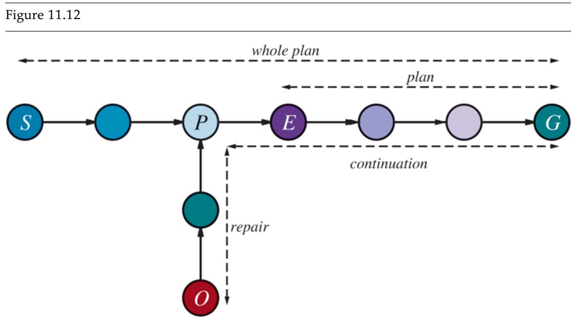
At first, the sequence “whole plan” is expected to get the agent from to . The agent executes steps of the plan until it expects to be in state , but observes that it is actually in . The agent then replans for the minimal repair plus continuation to reach .

Now let’s return to the example problem of achieving a chair and table of matching color. Suppose the agent comes up with this plan:

Now the agent is ready to execute the plan. The agent observes that the table and can of paint are white and the chair is black. It then executes . At this point a classical planner would declare victory; the plan has been executed. But an online execution monitoring agent needs to check that the action succeeded.

Suppose the agent perceives that the chair is a mottled gray because the black paint is showing through. The agent then needs to figure out a recovery position in the plan to aim for and a repair action sequence to get there. The agent notices that the current state is identical to the precondition before the action, so the agent chooses the empty sequence for repair and makes its plan be the same [Paint] sequence that it just attempted. With this new plan in place, execution monitoring resumes, and the Paint action is retried. This behavior will loop until the chair is perceived to be completely painted. But notice that the loop is created by a process of plan–execute–replan, rather than by an explicit loop in a plan. Note also that the original plan need not cover every contingency. If the agent reaches the step marked REPLAN, it can then generate a new plan (perhaps involving ).

Action monitoring is a simple method of execution monitoring, but it can sometimes lead to less than intelligent behavior. For example, suppose there is no black or white paint, and the agent constructs a plan to solve the painting problem by painting both the chair and table red. Suppose that there is only enough red paint for the chair. With action monitoring, the agent would go ahead and paint the chair red, then notice that it is out of paint and cannot paint the table, at which point it would replan a repair—perhaps painting both chair and table green. A plan-monitoring agent can detect failure whenever the current state is such that the remaining plan no longer works. Thus, it would not waste time painting the chair red.

Plan monitoring achieves this by checking the preconditions for success of the entire remaining plan—that is, the preconditions of each step in the plan, except those preconditions that are achieved by another step in the remaining plan. Plan monitoring cuts off execution of a doomed plan as soon as possible, rather than continuing until the failure actually occurs. Plan monitoring also allows for serendipity—accidental success. If someone comes along and paints the table red at the same time that the agent is painting the chair red, then the final plan preconditions are satisfied (the goal has been achieved), and the agent can go home early. 5

5 Plan monitoring means that finally, after 374 pages, we have an agent that is smarter than a dung beetle (see page 41). A planmonitoring agent would notice that the dung ball was missing from its grasp and would replan to get another ball and plug its hole. It is straightforward to modify a planning algorithm so that each action in the plan is annotated with the action’s preconditions, thus enabling action monitoring. It is slightly more complex to enable plan monitoring. Partial-order planners have the advantage that they have already built up structures that contain the relations necessary for plan monitoring. Augmenting state-space planners with the necessary annotations can be done by careful bookkeeping as the goal fluents are regressed through the plan.

Now that we have described a method for monitoring and replanning, we need to ask, “Does it work?” This is a surprisingly tricky question. If we mean, “Can we guarantee that the agent will always achieve the goal?” then the answer is no, because the agent could inadvertently arrive at a dead end from which there is no repair. For example, the vacuum agent might have a faulty model of itself and not know that its batteries can run out. Once they do, it cannot repair any plans. If we rule out dead ends—assume that there exists a plan to reach the goal from any state in the environment—and assume that the environment is really nondeterministic, in the sense that such a plan always has some chance of success on any given execution attempt, then the agent will eventually reach the goal.

Trouble occurs when a seemingly-nondeterministic action is not actually random, but rather depends on some precondition that the agent does not know about. For example, sometimes a paint can may be empty, so painting from that can has no effect. No amount of retrying is going to change this. One solution is to choose randomly from among the set of possible repair plans, rather than to try the same one each time. In this case, the repair plan of opening another can might work. A better approach is to learn a better model. Every prediction failure is an opportunity for learning; an agent should be able to modify its model of the world to accord with its percepts. From then on, the replanner will be able to come up with a repair that gets at the root problem, rather than relying on luck to choose a good repair. 6

6 Futile repetition of a plan repair is exactly the behavior exhibited by the sphex wasp (page 41).

11.6 Time, Schedules, and Resources

Classical planning talks about what to do, in what order, but does not talk about time: how long an action takes and when it occurs. For example, in the airport domain we could produce a plan saying what planes go where, carrying what, but could not specify departure and arrival times. This is the subject matter of scheduling.

Scheduling

The real world also imposes resource constraints: an airline has a limited number of staff, and staff who are on one flight cannot be on another at the same time. This section introduces techniques for planning and scheduling problems with resource constraints.

Resource constraint

The approach we take is “plan first, schedule later”: divide the overall problem into a planning phase in which actions are selected, with some ordering constraints, to meet the goals of the problem, and a later scheduling phase, in which temporal information is added to the plan to ensure that it meets resource and deadline constraints. This approach is common in real-world manufacturing and logistical settings, where the planning phase is sometimes automated, and sometimes performed by human experts.

11.6.1 Representing temporal and resource constraints

A typical job-shop scheduling problem (see Section 6.1.2 ), consists of a set of jobs, each of which has a collection of actions with ordering constraints among them. Each action has a duration and a set of resource constraints required by the action. A constraint specifies a type of resource (e.g., bolts, wrenches, or pilots), the number of that resource required, and whether that resource is consumable (e.g., the bolts are no longer available for use) or reusable (e.g., a pilot is occupied during a flight but is available again when the flight is over). Actions can also produce resources (e.g., manufacturing and resupply actions).

Job-shop scheduling problem
Job
Duration
Consumable

Reusable

A solution to a job-shop scheduling problem specifies the start times for each action and must satisfy all the temporal ordering constraints and resource constraints. As with search and planning problems, solutions can be evaluated according to a cost function; this can be quite complicated, with nonlinear resource costs, time-dependent delay costs, and so on. For simplicity, we assume that the cost function is just the total duration of the plan, which is called the makespan.

Makespan

Figure 11.13 shows a simple example: a problem involving the assembly of two cars. The problem consists of two jobs, each of the form [AddEngine,AddWheels, Inspect]. Then the Resources statement declares that there are four types of resources, and gives the number of each type available at the start: 1 engine hoist, 1 wheel station, 2 inspectors, and 500 lug nuts. The action schemas give the duration and resource needs of each action. The lug nuts are consumed as wheels are added to the car, whereas the other resources are “borrowed” at the start of an action and released at the action’s end.

Figure 11.13

Jobs({AddEngine1 < AddWheels1 < Inspect1}, AddEngine2 < AddWheels2 < Inspect2} }
Resources(EngineHoists(1), WheelStations(1), Inspectors(e2), LugNuts(500)
Action(AddEnginel, DURATION:30,
USE:EngineHoists(1))
Action(AddEngine2, DURATION:60,
USE:EngineHoists(1))
Action(AddWheels1, DURATION:30,
CONSUME:LugNuts(20), USE:WheelStations(1))
Action(AddWheels2, DURATION:15,
CONSUME:LugNuts(20), USE:WheelStations(1))
Action(Inspect;, DURATION:10,
USE:Inspectors(1))

A job-shop scheduling problem for assembling two cars, with resource constraints. The notation means that action must precede action .

The representation of resources as numerical quantities, such as Inspectors(2), rather than as named entities, such as and , is an example of a technique called aggregation: grouping individual objects into quantities when the objects are all indistinguishable. In our assembly problem, it does not matter which inspector inspects the car, so there is no need to make the distinction. Aggregation is essential for reducing complexity. Consider what happens when a proposed schedule has 10 concurrent Inspect actions but only 9 inspectors are available. With inspectors represented as quantities, a failure is detected immediately and the algorithm backtracks to try another schedule. With inspectors represented as individuals, the algorithm would try all ways of assigning inspectors to actions before noticing that none of them work.

Aggregation

11.6.2 Solving scheduling problems

We begin by considering just the temporal scheduling problem, ignoring resource constraints. To minimize makespan (plan duration), we must find the earliest start times for all the actions consistent with the ordering constraints supplied with the problem. It is helpful to view these ordering constraints as a directed graph relating the actions, as shown in Figure 11.14 . We can apply the critical path method (CPM) to this graph to determine the possible start and end times of each action. A path through a graph representing a partial-order plan is a linearly ordered sequence of actions beginning with Start and ending with Finish. (For example, there are two paths in the partial-order plan in Figure 11.14 .)

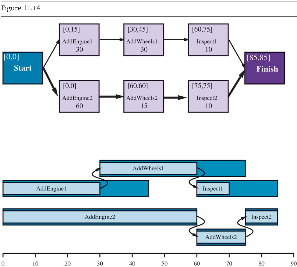
Top: a representation of the temporal constraints for the job-shop scheduling problem of Figure 11.13 . The duration of each action is given at the bottom of each rectangle. In solving the problem, we compute the earliest and latest start times as the pair , displayed in the upper left. The difference between these two numbers is the slack of an action; actions with zero slack are on the critical path, shown with bold arrows. Bottom: the same solution shown as a timeline. Grey rectangles represent time intervals during which an action may be executed, provided that the ordering constraints are respected. The unoccupied portion of a gray rectangle indicates the slack.

Critical path method

The critical path is that path whose total duration is longest; the path is “critical” because it determines the duration of the entire plan—shortening other paths doesn’t shorten the plan as a whole, but delaying the start of any action on the critical path slows down the whole plan. Actions that are off the critical path have a window of time in which they can be executed. The window is specified in terms of an earliest possible start time, , and a latest possible start time, . The quantity – is known as the slack of an action. We can see in Figure 11.14 that the whole plan will take 85 minutes, that each action in the top job has 15 minutes of slack, and that each action on the critical path has no slack (by definition). Together the and times for all the actions constitute a schedule for the problem.

Critical path

Slack

Schedule

The following formulas define and and constitute a dynamic-programming algorithm to compute them. and are actions, and means that precedes :

\[\begin{aligned} ES\left(Start\right) &= 0\\ ES\left(B\right) &= \max\_{A \prec B} ES\left(A\right) + Duration\left(A\right) \\ LS\left(Finish\right) &= ES\left(Finish\right) \\ LS\left(A\right) &= \min\_{B \prec A} LS\left(B\right) - Duration\left(A\right) \end{aligned}\]

The idea is that we start by assigning to be . Then, as soon as we get an action such that all the actions that come immediately before have values assigned, we set to be the maximum of the earliest finish times of those immediately preceding actions, where the earliest finish time of an action is defined as the earliest start time plus the duration. This process repeats until every action has been assigned an value. The values are computed in a similar manner, working backward from the Finish action.

The complexity of the critical path algorithm is just , where is the number of actions and is the maximum branching factor into or out of an action. (To see this, note that the and computations are done once for each action, and each computation iterates over at most other actions.) Therefore, finding a minimum-duration schedule, given a partial ordering on the actions and no resource constraints, is quite easy.

Mathematically speaking, critical-path problems are easy to solve because they are defined as a conjunction of linear inequalities on the start and end times. When we introduce resource constraints, the resulting constraints on start and end times become more complicated. For example, the AddEngine actions, which begin at the same time in Figure 11.14 , require the same EngineHoist and so cannot overlap. The “cannot overlap” constraint is a disjunction of two linear inequalities, one for each possible ordering. The introduction of disjunctions turns out to make scheduling with resource constraints NPhard.

Figure 11.15 shows the solution with the fastest completion time, 115 minutes. This is 30 minutes longer than the 85 minutes required for a schedule without resource constraints. Notice that there is no time at which both inspectors are required, so we can immediately move one of our two inspectors to a more productive position.

A solution to the job-shop scheduling problem from Figure 11.13 , taking into account resource constraints. The left-hand margin lists the three reusable resources, and actions are shown aligned horizontally with the resources they use. There are two possible schedules, depending on which assembly uses the engine hoist first; we’ve shown the shortest-duration solution, which takes 115 minutes.

There is a long history of work on optimal scheduling. A challenge problem posed in 1963 to find the optimal schedule for a problem involving just 10 machines and 10 jobs of 100 actions each—went unsolved for 23 years (Lawler et al. 1993). Many approaches have been tried, including branch-and-bound, simulated annealing, tabu search, and constraint satisfaction. One popular approach is the minimum slack heuristic: on each iteration, schedule for the earliest possible start whichever unscheduled action has all its predecessors scheduled and has the least slack; then update the and times for each affected action and repeat. This greedy heuristic resembles the minimum-remaining-values (MRV) heuristic in constraint satisfaction. It often works well in practice, but for our assembly problem it yields a 130-minute solution, not the 115-inute solution of Figure 11.15 .

Minimum slack

Up to this point, we have assumed that the set of actions and ordering constraints is fixed. Under these assumptions, every scheduling problem can be solved by a nonoverlapping sequence that avoids all resource conflicts, provided that each action is feasible by itself. However if a scheduling problem is proving very difficult, it may not be a good idea to solve it this way—it may be better to reconsider the actions and constraints, in case that leads to a much easier scheduling problem. Thus, it makes sense to integrate planning and scheduling by taking into account durations and overlaps during the construction of a plan. Several of the planning algorithms in Section 11.2 can be augmented to handle this information.

11.7 Analysis of Planning Approaches

Planning combines the two major areas of AI we have covered so far: search and logic. A planner can be seen either as a program that searches for a solution or as one that (constructively) proves the existence of a solution. The cross-fertilization of ideas from the two areas has allowed planners to scale up from toy problems where the number of actions and states was limited to around a dozen, to real-world industrial applications with millions of states and thousands of actions.

Planning is foremost an exercise in controlling combinatorial explosion. If there are propositions in a domain, then there are states. Against such pessimism, the identification of independent subproblems can be a powerful weapon. In the best case—full decomposability of the problem—we get an exponential speedup. Decomposability is destroyed, however, by negative interactions between actions. SATPLAN can encode logical relations between subproblems. Forward search addresses the problem heuristically by trying to find patterns (subsets of propositions) that cover the independent subproblems. Since this approach is heuristic, it can work even when the subproblems are not completely independent.

Unfortunately, we do not yet have a clear understanding of which techniques work best on which kinds of problems. Quite possibly, new techniques will emerge, perhaps providing a synthesis of highly expressive first-order and hierarchical representations with the highly efficient factored and propositional representations that dominate today. We are seeing examples of portfolio planning systems, where a collection of algorithms are available to apply to any given problem. This can be done selectively (the system classifies each new problem to choose the best algorithm for it), or in parallel (all the algorithms run concurrently, each on a different CPU), or by interleaving the algorithms according to a schedule.

Portfolio

Summary

In this chapter, we described the PDDL representation for both classical and extended planning problems, and presented several algorithmic approaches for finding solutions. The points to remember:

• Planning systems are problem-solving algorithms that operate on explicit factored representations of states and actions. These representations make possible the derivation of effective domain-independent heuristics and the development of powerful and flexible algorithms for solving problems.
• PDDL, the Planning Domain Definition Language, describes the initial and goal states as conjunctions of literals, and actions in terms of their preconditions and effects. Extensions represent time, resources, percepts, contingent plans, and hierarchical plans.
• State-space search can operate in the forward direction (progression) or the backward direction (regression). Effective heuristics can be derived by subgoal independence assumptions and by various relaxations of the planning problem.
• Other approaches include encoding a planning problem as a Boolean satisfiability problem or as a constraint satisfaction problem; and explicitly searching through the space of partially ordered plans.
• Hierarchical task network (HTN) planning allows the agent to take advice from the domain designer in the form of high-level actions (HLAs) that can be implemented in various ways by lower-level action sequences. The effects of HLAs can be defined with angelic semantics, allowing provably correct high-level plans to be derived without consideration of lower-level implementations. HTN methods can create the very large plans required by many real-world applications.
• Contingent plans allow the agent to sense the world during execution to decide what branch of the plan to follow. In some cases, sensorless or conformant planning can be used to construct a plan that works without the need for perception. Both conformant and contingent plans can be constructed by search in the space of belief states. Efficient representation or computation of belief states is a key problem.
• An online planning agent uses execution monitoring and splices in repairs as needed to recover from unexpected situations, which can be due to nondeterministic actions, exogenous events, or incorrect models of the environment.
• Many actions consume resources, such as money, gas, or raw materials. It is convenient to treat these resources as numeric measures in a pool rather than try to reason about, say, each individual coin and bill in the world. Time is one of the most important resources. It can be handled by specialized scheduling algorithms, or scheduling can be integrated with planning.
• This chapter extends classical planning to cover nondeterministic environments (where outcomes of actions are uncertain), but it is not the last word on planning. Chapter 17 describes techniques for stochastic environments (in which outcomes of actions have probabilities associated with them): Markov decision processes, partially observable Markov decision processes, and game theory. In Chapter 22 we show that reinforcement learning allows an agent to learn how to behave from past successes and failures.

Bibliographical and Historical Notes

AI planning arose from investigations into state-space search, theorem proving, and control theory. STRIPS (Fikes and Nilsson, 1971; 1993), the first major planning system, was designed as the planner for the Shakey robot at SRI. The first version of the program ran on a computer with only 192 KB of memory. Its overall control structure was modeled on GPS, the General Problem Solver (Newell and Simon, 1961), a state-space search system that used means–ends analysis.

The STRIPS representation language evolved into the Action Description Language, or ADL (Pednault, 1986), and then the Problem Domain Description Language, or PDDL (Ghallab et al. 1998), which has been used for the International Planning Competition since 1998. The most recent version is PDDL 3.1 (Kovacs, 2011).

Planners in the early 1970s decomposed problems by computing a subplan for each subgoal and then stringing the subplans together in some order. This approach, called linear planning by Sacerdoti (1975), was soon discovered to be incomplete. It cannot solve some very simple problems, such as the Sussman anomaly (see Exercise 11.SUSS), found by Allen Brown during experimentation with the HACKER system (Sussman, 1975). A complete planner must allow for interleaving of actions from different subplans within a single sequence. Warren’s (1974) WARPLAN system achieved that, and demonstrated how the logic programming language Prolog can produce concise programs; WARPLAN is only 100 lines of code.

Partial-order planning dominated the next 20 years of research, with theoretical work describing the detection of conflicts (Tate, 1975a) and the protection of achieved conditions (Sussman, 1975), and implementations including NOAH (Sacerdoti, 1977) and NONLIN (Tate, 1977). That led to formal models (Chapman, 1987; McAllester and Rosenblitt, 1991) that allowed for theoretical analysis of various algorithms and planning problems, and to a widely distributed system, UCPOP (Penberthy and Weld, 1992).

Drew McDermott suspected that the emphasis on partial-order planning was crowding out other techniques that should perhaps be reconsidered now that computers had 100 times the memory of Shakey’s day. His UNPOP (McDermott, 1996) was a state-space planning

program employing the ignore-delete-list heuristic. HSP, the Heuristic Search Planner (Bonet and Geffner, 1999; Haslum, 2006) made state-space search practical for large planning problems. The FF or Fast Forward planner (Hoffmann, 2001; Hoffmann and Nebel, 2001; Hoffmann, 2005) and the FASTDOWNWARD variant (Helmert, 2006) won international planning competitions in the 2000s.

Bidirectional search (see Section 3.4.5 ) has also been known to suffer from a lack of heuristics, but some success has been obtained by using backward search to create a perimeter around the goal, and then refining a heuristic to search forward towards that perimeter (Torralba et al. 2016). The SYMBA\* bidirectional search planner (Torralba et al. 2016) won the 2016 competition.

Researchers turned to PDDL and the planning paradigm so that they could use domain independent heuristics. Hoffmann (2005) analyzes the search space of the ignore-delete-list heuristic. Edelkamp (2009) and Haslum et al. (2007) describe how to construct pattern databases for planning heuristics. Felner et al. (2004) show encouraging results using pattern databases for sliding-tile puzzles, which can be thought of as a planning domain, but Hoffmann et al. (2006) show some limitations of abstraction for classical planning problems. (Rintanen, 2012) discusses planning-specific variable-selection heuristics for SAT solving.

Helmert et al. (2011) describe the Fast Downward Stone Soup (FDSS) system, a portfolio planner that, as in the fable of stone soup, invites us to throw in as many planning algorithms as possible. The system maintains a set of training problems, and for each problem and each algorithm records the run time and resulting plan cost of the problem’s solution. Then when faced with a new problem, it uses the past experience to decide which algorithm(s) to try, with what time limits, and takes the solution with minimal cost. FDSS was a winner in the 2018 International Planning Competition (Seipp and Röger, 2018). Seipp et al. (2015) describe a machine learning approach to automatically learn a good portfolio, given a new problem. Vallati et al. (2015) give an overview of portfolio planning. The idea of algorithm portfolios for combinatorial search problems goes back to Gomes and Selman, (2001).

Sistla and Godefroid (2004) cover symmetry reduction, and Godefroid (1990) covers heuristics for partial ordering. Richter and Helmert (2009) demonstrate the efficiency gains of forward pruning using preferred actions.

Blum and Furst (1997) revitalized the field of planning with their Graphplan system, which was orders of magnitude faster than the partial-order planners of the time. Bryce and Kambhampati (2007) give an overview of planning graphs. The use of situation calculus for planning was introduced by John McCarthy (1963) and refined by Ray Reiter (2001).

Kautz et al. (1996) investigated various ways to propositionalize action schemas, finding that the most compact forms did not necessarily lead to the fastest solution times. A systematic analysis was carried out by Ernst et al. (1997), who also developed an automatic “compiler” for generating propositional representations from PDDL problems. The BLACKBOX planner, which combines ideas from Graphplan and SATPLAN, was developed by Kautz and Selman (1998). Planners based on constraint satisfaction include CPLAN van Beek and Chen (1999) and GP-CSP (Do and Kambhampati, 2003).

There has also been interest in the representation of a plan as a binary decision diagram (BDD), a compact data structure for Boolean expressions widely studied in the hardware verification community (Clarke and Grumberg, 1987; McMillan, 1993). There are techniques for proving properties of binary decision diagrams, including the property of being a solution to a planning problem. Cimatti et al. (1998) present a planner based on this approach. Other representations have also been used, such as integer programming (Vossen et al. 2001).

Binary decision diagram (BDD)

There are some interesting comparisons of the various approaches to planning. Helmert (2001) analyzes several classes of planning problems, and shows that constraint-based approaches such as Graphplan and SATPLAN are best for NP-hard domains, while searchbased approaches do better in domains where feasible solutions can be found without backtracking. Graphplan and SATPLAN have trouble in domains with many objects because that means they must create many actions. In some cases the problem can be delayed or avoided by generating the propositionalized actions dynamically, only as needed, rather than instantiating them all before the search begins.

The first mechanism for hierarchical planning was a facility in the STRIPS program for learning macrops—“macro-operators” consisting of a sequence of primitive steps (Fikes et al. 1972). The ABSTRIPS system (Sacerdoti, 1974) introduced the idea of an abstraction hierarchy, whereby planning at higher levels was permitted to ignore lower-level preconditions of actions in order to derive the general structure of a working plan. Austin Tate’s Ph.D. thesis (1975b) and work by Earl Sacerdoti (1977) developed the basic ideas of HTN planning. Erol, Hendler, and Nau (1994, 1996) present a complete hierarchical decomposition planner as well as a range of complexity results for pure HTN planners. Our presentation of HLAs and angelic semantics is due to Marthi et al. (2007, 2008).

Macrops

Abstraction hierarchy

One of the goals of hierarchical planning has been the reuse of previous planning experience in the form of generalized plans. The technique of explanation-based learning has been used as a means of generalizing previously computed plans in systems such as SOAR (Laird et al. 1986) and PRODIGY (Carbonell et al. 1989). An alternative approach is to store previously computed plans in their original form and then reuse them to solve new, similar problems by analogy to the original problem. This is the approach taken by the field called case-based planning (Carbonell, 1983; Alterman, 1988). Kambhampati (1994) argues that case-based planning should be analyzed as a form of refinement planning and provides a formal foundation for case-based partial-order planning.

Case-based planning

Early planners lacked conditionals and loops, but some could use coercion to form conformant plans. Sacerdoti’s NOAH solved the “keys and boxes” problem (in which the planner knows little about the initial state) using coercion. Mason (1993) argued that sensing often can and should be dispensed with in robotic planning, and described a sensorless plan that can move a tool into a specific position on a table by a sequence of tilting actions, regardless of the initial position.

Goldman and Boddy (1996) introduced the term conformant planning, noting that sensorless plans are often effective even if the agent has sensors. The first moderately efficient conformant planner was Smith and Weld’s (1998) Conformant Graphplan (CGP). Ferraris and Giunchiglia (2000) and Rintanen (1999) independently developed SATPLANbased conformant planners. Bonet and Geffner (2000) describe a conformant planner based on heuristic search in the space of belief states, drawing on ideas first developed in the 1960s for partially observable Markov decision processes, or POMDPs (see Chapter 17 ).

Currently, there are three main approaches to conformant planning. The first two use heuristic search in belief-state space: HSCP (Bertoli et al. 2001a) uses binary decision diagrams (BDDs) to represent belief states, whereas Hoffmann and Brafman (2006) adopt the lazy approach of computing precondition and goal tests on demand using a SAT solver.

The third approach, championed primarily by Jussi Rintanen (2007), formulates the entire sensorless planning problem as a quantified Boolean formula (QBF) and solves it using a general-purpose QBF solver. Current conformant planners are five orders of magnitude faster than CGP. The winner of the 2006 conformant-planning track at the International Planning Competition was (Palacios and Geffner, 2007), which uses heuristic search in belief-state space while keeping the belief-state representation simple by defining derived literals that cover conditional effects. Bryce and Kambhampati (2007) discuss how a planning graph can be generalized to generate good heuristics for conformant and contingent planning.

The contingent-planning approach described in the chapter is based on Hoffmann and Brafman (2005), and was influenced by the efficient search algorithms for cyclic AND–OR graphs developed by Jimenez and Torras (2000) and Hansen and Zilberstein (2001). The problem of contingent planning received more attention after the publication of Drew McDermott’s (1978a) influential article, Planning and Acting. Bertoli et al. (2001b) describe MBP (Model-Based Planner), which uses binary decision diagrams to do conformant and contingent planning. Some authors use “conditional planning” and “contingent planning” as synonyms; others make the distinction that “conditional” refers to actions with nondeterministic effects, and “contingent” means using sensing to overcome partial observability.

In retrospect, it is now possible to see how the major classical planning algorithms led to extended versions for uncertain domains. Fast-forward heuristic search through state space led to forward search in belief space (Bonet and Geffner, 2000; Hoffmann and Brafman, 2005); SATPLAN led to stochastic SATPLAN (Majercik and Littman, 2003) and to planning with quantified Boolean logic (Rintanen, 2007); partial order planning led to UWL (Etzioni et al. 1992) and CNLP (Peot and Smith, 1992); Graphplan led to Sensory Graphplan or SGP (Weld et al. 1998).

The first online planner with execution monitoring was PLANEX (Fikes et al. 1972), which worked with the STRIPS planner to control the robot Shakey. SIPE (System for Interactive Planning and Execution monitoring) (Wilkins, 1988) was the first planner to deal systematically with the problem of replanning. It has been used in demonstration projects in several domains, including planning operations on the flight deck of an aircraft carrier, jobshop scheduling for an Australian beer factory, and planning the construction of multistory buildings (Kartam and Levitt, 1990).

In the mid-1980s, pessimism about the slow run times of planning systems led to the proposal of reflex agents called reactive planning systems (Brooks, 1986; Agre and Chapman, 1987). “Universal plans” (Schoppers, 1989) were developed as a lookup-table method for reactive planning, but turned out to be a rediscovery of the idea of policies that had long been used in Markov decision processes (see Chapter 17 ). Koenig (2001) surveys online planning techniques, under the name Agent-Centered Search.

Reactive planning

Planning with time constraints was first dealt with by DEVISER (Vere, 1983). The representation of time in plans was addressed by Allen (1984) and by Dean et al. (1990) in the FORBIN system. NONLIN+ (Tate and Whiter, 1984) and SIPE (Wilkins, 1990) could reason about the allocation of limited resources to various plan steps. O-PLAN (Bell and Tate, 1985) has been applied to resource problems such as software procurement planning at Price Waterhouse and back-axle assembly planning at Jaguar Cars.

The two planners SAPA (Do and Kambhampati, 2001) and T4 (Haslum and Geffner, 2001) both used forward state-space search with sophisticated heuristics to handle actions with durations and resources. An alternative is to use very expressive action languages, but guide them by human-written, domain-specific heuristics, as is done by ASPEN (Fukunaga et al. 1997), HSTS (Jonsson et al. 2000), and IxTeT (Ghallab and Laruelle, 1994).

A number of hybrid planning-and-scheduling systems have been deployed: ISIS (Fox et al. 1982; Fox, 1990) has been used for job-shop scheduling at Westinghouse, GARI (Descotte and Latombe, 1985) planned the machining and construction of mechanical parts, FORBIN was used for factory control, and NONLIN+ was used for naval logistics planning. We chose to present planning and scheduling as two separate problems; Cushing et al. (2007) show that this can lead to incompleteness on certain problems.

There is a long history of scheduling in aerospace. T-SCHED (Drabble, 1990) was used to schedule mission-command sequences for the UOSAT-II satellite. OPTIMUM-AIV (Aarup et al. 1994) and PLAN-ERS1 (Fuchs et al. 1990), both based on O-PLAN, were used for spacecraft assembly and observation planning, respectively, at the European Space Agency. SPIKE (Johnston and Adorf, 1992) was used for observation planning at NASA for the Hubble Space Telescope, while the Space Shuttle Ground Processing Scheduling System (Deale et al. 1994) does job-shop scheduling of up to 16,000 worker-shifts. Remote Agent (Muscettola et al. 1998) became the first autonomous planner–scheduler to control a spacecraft, when it flew onboard the Deep Space One probe in 1999. Space applications have driven the development of algorithms for resource allocation; see Laborie (2003) and Muscettola (2002). The literature on scheduling is presented in a classic survey article (Lawler et al. 1993), a book (Pinedo, 2008), and an edited handbook (Blazewicz et al. 2007).

The computational complexity of of planning has been analyzed by several authors (Bylander, 1994; Ghallab et al. 2004; Rintanen, 2016). There are two main tasks: PlanSAT is the question of whether there exists any plan that solves a planning problem. Bounded PlanSAT asks whether there is a solution of length or less; this can be used to find an optimal plan. Both are decidable for classical planning (because the number of states is finite). But if we add function symbols to the language, then the number of states becomes infinite, and PlanSAT becomes only semidecidable. For propositionalized problems both are in the complexity class PSPACE, a class that is larger (and hence more difficult) than NP and refers to problems that can be solved by a deterministic Turing machine with a polynomial amount of space. These theoretical results are discouraging, but in practice, the problems we want to solve tend to be not so bad. The true advantage of the classical planning formalism is that it has facilitated the development of very accurate domain-independent heuristics; other approaches have not been as fruitful.

Readings in Planning (Allen et al. 1990) is a comprehensive anthology of early work in the field. Weld (1994, 1999) provides two excellent surveys of planning algorithms of the 1990s. It is interesting to see the change in the five years between the two surveys: the first concentrates on partial-order planning, and the second introduces Graphplan and SATPLAN. Automated Planning and Acting (Ghallab et al. 2016) is an excellent textbook on all aspects of the field. LaValle’s text Planning Algorithms (2006) covers both classical and stochastic planning, with extensive coverage of robot motion planning.

Planning research has been central to AI since its inception, and papers on planning are a staple of mainstream AI journals and conferences. There are also specialized conferences such as the International Conference on Automated Planning and Scheduling and the International Workshop on Planning and Scheduling for Space.